mining conflgurable enterprise information systems -...
TRANSCRIPT
Mining Configurable Enterprise Information
Systems
M.H. Jansen-Vullers a W.M.P. van der Aalst a M. Rosemann b
aDepartment of Technology Management, Eindhoven University of Technology,P.O. Box 513, NL-5600 MB, Eindhoven, The Netherlands.
bFaculty of Information Technology, Queensland University of Technology, 126Margaret Street Brisbane Qld 4000, Australia.
Abstract
Process mining is the extraction of a process model from system logs. These logshave to meet minimum requirements, i.e. each event should refer to a case and a task.Many system logs do not meet these requirements, and therefore it is not possibleto use process mining for process optimization or delta analysis. This paper showsan alternative process mining procedure for logs containing data on the frequencythat process steps have been executed. To be able to mine such logs we applyConfigurable Event-driven Process Chains (C-EPCs). If a C-EPC is available, wepropose a method to mine the process. If only a classical reference model (i.e. anEPC) is available, we propose a method to first derive the C-EPC through miningand then analyse the process. This approach enables us to do process mining in thecontext of ERP systems such as SAP R/3.
Key words: Data and Process Re-engineering, Data Mining, KnowledgeDiscovery, Reference Models, Enterprise Information Systems
1 Introduction
Many organizations are confronted with problems resulting from badly imple-mented enterprise information systems. They observe that the system frus-trates the normal way of handling processes. Maybe the system is not able tosupport the process as it should be carried out, or maybe the business process
Email addresses: [email protected] (M.H. Jansen-Vullers),[email protected] (W.M.P. van der Aalst), [email protected](M. Rosemann).
Preprint submitted to Elsevier Preprint 27 April 2004
as implemented in the enterprise information system is not known or acceptedby the employees [30]. As a result, the actual business process may divergefrom the processes as implemented in the enterprise information system. Toimprove such a situation, it would be helpful to know the actual steps whencarrying out a particular process. Process mining can do this as the actualprocess is taken as a starting point [5].
Other areas where process mining might contribute are reconfiguration orupgrades of configurable enterprise information systems. When an enterpriseinformation system is in use for some time, typically quite a number of updatesand extensions have been added. Documentation, if present at all, is outdated.When mining the actual processes from the old system, the result can beused to implement the new system, without requiring too much effort fromscarce resources [28]. Apart from finding the actual process or making a deltaanalysis, process mining allows for performance analysis by explicitly definingthe executed processes.
Process mining is well-described in literature, see e.g. [5,6,9,15–17,24,25,36–38,42–44]. Process mining requires logs from enterprise information systemssuch as workflow management systems, case-handling systems and EnterpriseResource Planning Systems. These logs may record several attributes, e.g. thecase that is being handled, the task and event types, the user that carried outthe task etc. It is not necessary that all information is available in the log, butthe reference to both cases and tasks is required.
This paper focuses on mining actual processes from incomplete logs, this iswithout both case and task reference. An example of such an incomplete log isa frequency profile, based on the frequency a transaction has been executed,e.g. task A has been carried out 100 times and task B 40 times (see left-hand side of Figure 1). As a result, pure process mining, this is without anyprior information about the process structure, is not possible. We need someadditional information in the form of process models such as best practicesor reference models [39,40]. We discuss how reference models (especially C-EPCs [32]) can contribute to mine actual processes. Our first research questionfocuses on the transformation process of a C-EPC and a frequency profile intoa configuration and a process model. In Figure 1 this process is illustrated.
However, if such a C-EPC is not available, we could use a more general ref-erence model, such as an EPC. Together with the frequency profile, a C-EPCand the actual process model can be determined. The second research questionfocuses on this transformation step. It should be taken into account that thederived C-EPC is merely based on one particular log and might differ fromC-EPCs based on other logs.
An extension of the previous approach is to take n logs, resulting in a set of
2

Task frequency
A 100
B 40
C 60
D 100
Frequency profile and C-EPC configuration and process model
c 1
c 2
c 3
c 4
B C
A
V
V
V
V
D
conf f D
=ON
conf c 2
=XOR
conf c3
=XOR
c 1
c 2
c 3
c 4
B C
A
X
X
V
V
D
Fig. 1. Process mining based on a frequency profile and an EPC (for elaboration ofthis example we refer to Section 4)
n C-EPCs. Subsequently, this set of C-EPCs can be consolidated into a moregeneral and more accurate C-EPC. This is the focus of the third researchquestion. The C-EPC can be improved by rules, e.g. a particular configurationsetting in one part of the model implies a particular setting in another partof the model.
Ultimately, the C-EPC can be extended by guidelines. Apart from the ref-erence model and n logs, additional meta data is required, such as cost andperformance data of the process, size of the company or the industry sector.Another extension can be the use of additional data in the log (time andresource of each event is known).
The paper is structured as follows. In the next section we present the back-ground of the research: process mining, its applicability to configurable en-terprise information systems and the role reference models might play miningthese systems. In our approach, we make extensive use of reference models,and especially EPCs and C-EPCs. The semantics of these modelling languagesshould be defined unambiguously, therefore EPCs and C-EPCs are formallydescribed in Section 3. Readers already familiar with this material could skipthis section. When elaborating the first research question, taking a C-EPCand a frequency profile as a starting point (Section 4), we will show that wecan apply existing software packages to support solving our mining problems;these software packages are based on Integer Programming techniques. In Sec-tion 5 we reformulate our approach in such a way that it indeed correspondsto an Integer Programming problem. When elaborating the other two researchquestions, i.e. starting from an EPC and one respectively n frequency profiles(Section 6) we will show that the solutions are variants of the solution of thefirst research question. This paper concludes with a section on related work,a brief summary and future work.
3

2 Background
2.1 Process Mining
During the last decade explicit process concepts (e.g. workflow models) havebeen applied in many enterprise information systems [3,12,20,23]. WorkflowManagement (WFM) Systems such as Staffware, IBM MQ-Series, COSA, etc.offer generic modelling and enactment capabilities for structured business pro-cesses. By making graphical process definitions, i.e. models describing the life-cycle of a particular case (process instance) in isolation, one can configurethese systems to support business processes. Many other systems make use ofexplicit process models. Consider for example Enterprise Resource Planningsystems (e.g. SAP, Peoplesoft, Baan and Oracle) or Customer RelationshipManagement software (Siebel), etc. As pointed out in the introduction, theactual collection of runtime process execution data from such Enterpise Infor-mation Systems may contribute to diagnoses, design and redesign of EnterpiseInformation Systems and business processes. The collection of runtime dataand the analysis of these data is called process mining.
For this mining process, the data logs of an enterprise information systemare processed by a mining tool, e.g. EMiT, Little Thumb, Process Miner, etc.[5]. The mining tools are generic, i.e. can be applied to all kinds of businessprocesses and all kinds of enterprise information systems. These tools require acommon XML format for storing and exchanging the logs. We have developedsuch a format, which is described by a document type definition (DTD) of anXML-schema (both can be downloaded from www.processmining.org). Figure2 shows that the XML-format connects the transactional systems such asworkflow systems, ERP systems, CRM systems etc. The XML-format is thenused as input for the mining tools. The goal of using a single format is to reducethe implementation effort and to promote the use of the mining concepts inmultiple contexts.
Application of the mining tools require logs in the specified format. Further-more, we assume that (1) each event refers to a task or well-defined step, (2)each event refers to a case or instance and (3) events are totally ordered. Ifthis is available, mining algorithms can be used to derive models describingthe underlying process. The minimum information (i.e. task and case) may becomplemented by resource, time, event type etc., thus allowing for the discov-ery of organizational structures, social networks and performance indicators.
Figure 3 shows an example log of a process from the workflow managementsystem Staffware. This log contains the required data case-id and task-id, andadditionally the event type (the task is scheduled, processed or released), the
4

Staffware
InConcert
MQ Series
workflow management systems
FLOWer
Vectus
Siebel
case handling / CRM systems
SAP R/3
BaaN
Peoplesoft
ERP systems
common XML format for storing/
exchanging workflow logs
EMiT Little
Thumb
mining tools
InWoLvE Process
Miner
Exper-
DiTo
Fig. 2. The XML-format as solver/system independent medium (available fromwww.processmining.org)
user and a time stamp.
Case 3 Step Description Event User yyyy/mm/dd hh:mm
----------------------------------------------------------------------------
Start mhjansen@staffw_ 2003/05/06 15:22
A Processed To mhjansen@staffw_ 2003/05/06 15:22
A Released By mhjansen@staffw_ 2003/05/06 15:22
C Processed To mhjansen@staffw_ 2003/05/06 15:22
C Released By mhjan sen@staffw_ 2003/05/06 15:22
D Processed To mhjansen@staffw_ 2003/05/06 15:22
D Released By mhjansen@staffw_ 2003/05/06 15:23
Terminated 2003/05/06 15:2 4
Case 1
Step Description Event User yyyy/mm/dd hh:mm
----------------------------------------------------------------------------
Start mhjansen@staffw_ 2003/05/06 15:22
A Processed To mhjansen@staffw_ 2003/05/06 15:22
A Released By mhjansen@staffw_ 2003/05/06 15:22
B Processed To mhjansen@staffw_ 2003/05/06 15:22
B Released By mhj ansen@staffw_ 2003/05/06 15:22
D Processed To mhjansen@staffw_ 2003/05/06 15:22
D Released By mhjansen@staffw_ 2003/05/06 15:23
Terminated 2003/05/06 15 :28
Case 2
Step Description Event User yyyy/mm/dd hh:mm
----------------------------------------------------------------------------
Start mhjansen@staffw_ 2003/05/06 15:22
A Processed To mhjansen@staffw_ 2003/05/06 15:22
A Released By mhjansen@staffw_ 2003/05/06 15:22
B Processed To mhjansen@staffw_ 2003/05/06 15:22
B Released By m hjansen@staffw_ 2003/05/06 15:23
D Processed To mhjansen@staffw_ 2003/05/06 15:23
D Released By mhjansen@staffw_ 2003/05/06 15:24
Terminated 2003/05/06 15:28
Fig. 3. Example log (based on the EPC in Figure 4)
However, for many types of systems the logs may look differently. Althoughfrom a pure process mining view such a log is incomplete, other data maybe available to help mining the actual process model. In the next subsection,we elaborate two alternative approaches to show which information in config-urable enterprise information systems might contribute to process mining.
5

2.2 Alternative approaches
When mining processes in enterprise information systems, the mining pro-cess is straightforward if data on the level of business process managementis available, e.g. like in Figure 3. If this type of information is not available,other data might help. We consider two types of registrations: (1) transactiondata stored in tables and (2) process registration in the context of databaseperformance.
Enterprise information systems make extensive use of the database that sup-ports the system: each business transaction results in a system transactionthat is recorded in the database. The data that is recorded are documentsthat are created or updated, such as purchase requisitions, purchase orders orscheduling agreements. In relation to these documents all other detailed trans-action data is stored in the database. Making use of these data is promisingin the context of process mining: the document numbers can be consideredas case-id. The derivation of the tasks that have been executed to create orupdate these documents is less straightforward, but may be possible. Thisapproach is used in tools such as ARIS Process Performance Manager (PPM)when analyzing process performance of SAP-supported business processes.
A disadvantage of this approach is that it is time consuming and very specific.For each particular process and variant of a process, it is necessary to findthe relevant tables and table fields. Additionally, this approach is sensitivewith respect to the configuration of the enterprise information system. Theactual configuration of the system may influence the use of tables and fields.To be able to pinpoint the exact table fields that are affected by a particularprocess, it is necessary to examine whether these fields may differ for particularconfigurations. Eventually, this may even lead to a mining approach in whichthe actual process should be known completely before mining the process.In PPM for example, we see that application of the software first requirescustomization of PPM [19]. In this manual step a consultant discusses theactual process with the process owner, which is input for PPM and thus theperformance analysis. The quality of the output of the performance analysis is,amongst others dependent on the quality of the model and the configurationof PPM.
Another approach originates from the fact that enterprise information systemssuch as SAP R/3 log data to be able to analyse the workload of the database.The workload analysis collects the workload of each transaction carried out inthe system. The workload analysis of a particular period summarizes whichtransactions have been carried out, by whom and how much computing timeit consumed. Tools like the SAP Reverse Business Engineer (RBE) make useof this feature and are able to report the transaction frequencies [28,34]. We
6

can apply this approach for process mining when deriving the frequencies ofthe execution of transactions. Unfortunately, there is no link between case-ids(document numbers) and these frequencies. In this context reference modelsmay contribute. A well-known example of such reference models are EventDriven Process chains (EPC’s) which have been developed in a collaborativeresearch project conducted by SAP AG and the IDS Scheer AG [21,35] andwhich form the basis of the SAP R/3 reference models [10]. Also other enter-prise information systems make use of similar reference models, e.g. Baan [41]or Intentia [13]. In this paper, we elaborate on this second approach. There-fore, in the next subsection we focus on the application of reference modelsfor process mining.
2.3 Reference models
Business process management frequently uses models, e.g. for modelling theenterprise, for information system specification or end-user training [7,14,31].These models may be descriptive or prescriptive. A typical example are refer-ence models in the context of Enterprise Resource Planning systems such asSAP. The SAP R/3 reference models are expressed in so-called Event-drivenProcess Chains (EPCs). Figure 4 shows an example of an EPC for internalorder handling.
1
A
2
X
C B
5
3
6
Check order
Product C
required
Product B
required
Manufacture
product C
Manufacture
product B
Order
received
Product C
available Product B
available
Deliver order
X
4
Order
delivered
D
Fig. 4. Example EPC
It should be taken into account that reference models for enterprise informa-tion systems such as SAP R/3 are extremely complex because of the com-
7

plexity of the business processes at one hand, and the fact that these systemsare configurable at the other hand. In fact, such a reference model (or EPC)is an ‘upperbound’ of process models that may possibly be implemented ina particular enterprise. Consider for example an enterprise information sys-tem that allows configuration of the purchasing process with respect to thequotation process. The related reference model consists of two branches (pro-curement with respectively without quotations). Some companies might notimplement quotations and it is clear which part of the process model is rele-vant. Other companies however, might implement the quotation functionality,though leaving implicit whether quotations are required (one branch of theprocess model is applicable) or quotations may be used which may dependenton some criteria (both branches of the process model are applicable). Becausesuch implicit decisions cannot be derived from such reference models, we callthese ‘upperbound’ or ‘maximum’ reference models (for example EPC-Max).
To handle the complexity that is caused by the possibility to configure asystem, a new approach has been developed that intuitively reflects the con-figurable nature of the enterprise information system. The representation ofthis reference modelling language is called configurable EPC (C-EPC) [32]. Inthis paper we will look at this specific class of reference models. In a C-EPC,there is an explicit distinction between choices made at runtime and choicesmade at configuration time. The following example illustrates the differencebetween these two types of decisions.
The left-hand side of Figure 5 shows an example of a C-EPC for transmittingpurchase orders. The configurable XOR-connector is used to state that atconfiguration time it should be decided whether executing both the left and theright branch, i.e. purchasing with or without scheduling agreements, is allowedfor a particular company. In the C-EPC this is modelled as configurable XOR-connector, which can be set XOR (i.e. choice and runtime); this is depictedin the middle part of Figure 5 (variant 1). In practice one may also findcompanies that do not allow purchase order processing based on schedulingagreements. In that case only one path can be selected (i.e. choice made atconfiguration time); this is depicted in the right-hand part of Figure 5 (variant2). This example is taken from [32] and is based on the SAP Reference ModelPurchasing, version 4.6c. For more details on the C-EPC approach we refer toSection 3.
8

Requisition
released
for SA
Scheduling
Agreement
Delivery
Purchase
requisition
released for
PO
Purchase
order
Creation
SA release
created
Purchase
order
created
Release of
purchase
order
Purchasing
document
released
X
Scheduling
Agreement
Delivery
Purchase
order
Processing
Purchasing
order
transmitted
Purchase
requisition
released for
PO
Purchase
order
Creation
Purchase
order
created
Release of
purchase
order
Purchasing
document
released
Purchase
order
Processing
Purchasing
order
transmitted
C-EPC Variant 1 Variant 2
Fig. 5. Example of a C-EPC with XOR-join (SA-scheduling agreement, PO - pur-chase order)
3 Formalization of EPCs and C-EPCs
3.1 Event-driven Process Chains
An Event-driven Process Chain (EPC) consists of events, functions and con-nectors. However, not every diagram composed of events, functions and con-nectors is a correct EPC. For example, it is not allowed to connect two eventsto each other (cf. [21]). Unfortunately, a formal syntax for event-driven processchains is missing. In this section, we give a formal definition of an event-drivenprocess chain. This definition is based on the restrictions described in [21] andimposed by tools such as ARIS and SAP R/3. This way we are able to specifythe requirements an event-driven process chain should satisfy.
Definition 1 (Event-driven process chain (1)) An event-driven processchain is a five-tuple (E, F, C, l, A):
- E is a finite set of events,- F is a finite set of functions,- C is a finite set of logical connectors,- l ∈ C → {∧,XOR,∨} is a function which maps each connector onto a
9

connector type,- A ⊆ (E×F )∪ (F ×E)∪ (E×C)∪ (C ×E)∪ (F ×C)∪ (C ×F )∪ (C ×C)
is a set of arcs.
An event-driven process chain is composed of three types of nodes: events (E),functions (F ) and connectors (C). The type of each connector is given by thefunction l: l(c) is the type (∧, XOR, or ∨) of a connector c ∈ C. Relation Aspecifies the set of arcs connecting functions, events and connectors. Definition1 shows that it is not allowed to have an arc connecting two functions ortwo events. There are many more requirements an event-driven process chainshould satisfy, e.g., only connectors are allowed to branch, there is at least onestart event, there is at least one final event, and there are several limitationswith respect to the use of connectors. To formalize these requirements we needto define some additional concepts and introduce some notation.
Definition 2 (Directed path and elementary path) Let EPC be an event-driven process chain. A directed path p from a node n1 to a node nk is asequence 〈n1, n2, . . . , nk〉 such that 〈ni, ni+1〉 ∈ A for 1 ≤ i ≤ k − 1. p iselementary iff for any two nodes ni and nj on p, i 6= j ⇒ ni 6= nj.
The definition of directed path will be used to limit the set of routing con-structs that may be used. It also allows for the definition of CEF (the set ofconnectors on a path from an event to a function) and CFE (the set of connec-tors on a path from a function to an event). CEF and CFE partition the setof connectors C. Based on the function l we also partition C into C∧, C∨, andCXOR. The sets CJ and CS are used to classify connectors into join connectorsand split connectors.
Definition 3 (N , C∧, C∨, CXOR, •, CJ , CS, CEF , CFE) Let EPC =(E, F, C, l, A) be an event-driven process chain.
- N = E ∪ F ∪ C is the set of nodes of EPC .- C∧ = {c ∈ C | l(c) = ∧}- C∨ = {c ∈ C | l(c) = ∨}- CXOR = {c ∈ C | l(c) = XOR}- For n ∈ N :•n = {m | (m,n) ∈ A} is the set of input nodes, andn• = {m | (n,m) ∈ A} is the set of output nodes.
- CJ = {c ∈ C | | • c| ≥ 2} is the set of join connectors.- CS = {c ∈ C | |c • | ≥ 2} is the set of split connectors.- CEF ⊆ C such that c ∈ CEF if and only if there is a path p = 〈n1, n2, . . . ,
nk−1, nk〉 such that n1 ∈ E, n2, . . . , nk−1 ∈ C, nk ∈ F , and c ∈ {n2, . . . ,nk−1}.
- CFE ⊆ C such that c ∈ CFE if and only if there is a path p = 〈n1, n2, . . . ,nk−1, nk〉 such that n1 ∈ F , n2, . . . , nk−1 ∈ C, nk ∈ E, and c ∈ {n2, . . . ,
10
nk−1}.
These notations allow for the completion of the definition of an event-drivenprocess chain.
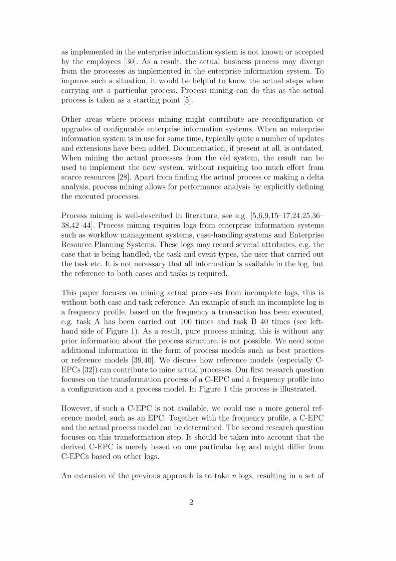
Definition 4 (Event-driven process chain (2)) An event-driven processchain EPC = (E, F, C, l, A) satisfies the following requirements:
- The sets E, F , and C are pairwise disjoint, i.e., E ∩ F = ∅, E ∩ C = ∅,and F ∩ C = ∅.
- For each e ∈ E: | • e| ≤ 1 and |e • | ≤ 1.- There is at least one event e ∈ E such that | • e| = 0 (i.e. a start event).- There is at least one event e ∈ E such that |e • | = 0 (i.e. a final event).- For each f ∈ F : | • f | = 1 and |f • | = 1.- For each c ∈ C: | • c| ≥ 1 or |c • | ≥ 1.- CJ and CS partition C, i.e., CJ ∩ CS = ∅ and CJ ∪ CS = C.- CEF and CFE partition C, i.e., CEF ∩ CFE = ∅ and CEF ∪ CFE = C.
The first requirement states that each component has a unique identifier(name). Note that connector names are omitted in the diagram of an event-driven process chain. The other requirements correspond to restrictions onthe relation A. Events cannot have multiple input arcs and there is at leastone start event and one final event. Each function has exactly one input arcand one output arc. A connector c is either a join connector (|c • | = 1 and| • c| ≥ 2) or a split connector (| • c| = 1 and |c • | ≥ 2). The last requirementstates that a connector c is either on a path from an event to a function or ona path from a function to an event. In the remainder of this paper we assumeall event-driven process chains to be syntactically correct.
Note that {CJ , CS}, {CEF , CFE}, and {C∧, CXOR, C∨} partition C, i.e., CJ andCS are disjoint and C = CJ ∪ CS, CEF and CFE are disjoint and C = CEF ∪CFE, and C∧, CXOR and C∨ are pair-wise disjoint and C = C∧ ∪ CXOR ∪ C∨.In principle there are 2× 2× 3 = 12 kinds of connectors! In [21] two of these12 constructs are not allowed: a split connector of type CEF cannot be of typeXOR or ∨, i.e., CS ∩CEF ∩CXOR = ∅ and CS ∩CEF ∩C∨ = ∅. As a result ofthis restriction, there are no choices between functions sharing the same inputevent. A choice is resolved after the execution of a function, not before. In thispaper, we will not impose this restriction.
The semantics of EPCs have often been debated in literature. Here we do notcontribute to this discussion but simply refer to [1,2,11,22,29,33].
11
3.2 Configurable EPCs
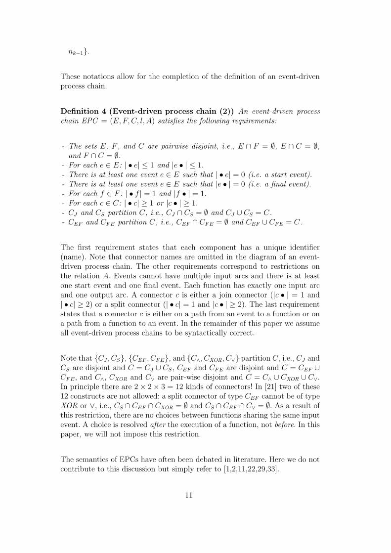
This section introduces the notion of a configurable event-driven process chainC-EPC. In a C-EPC functions and connectors can be configurable. Con-figurable functions may be included (ON ), skipped (OFF ) or conditionallyskipped (OPT ). Configurable connectors may be restricted at configurationtime, e.g., a configurable connector of type ∨ may be mapped onto a ∧ con-nector. Local configuration choices like skipping a function may be limitedby configuration requirements. For example, if one configurable connector oftype ∨ is mapped onto ∧ connector, then another configurable function needsto be included. This configuration requirement may be denoted by the logi-cal expression c = ∧ ⇒ f = ON . To guide the configuration process thereis also a partial order which suggests the order of configuration. Moreover,besides the configuration requirements there may also be configuration guide-lines. One can think of configuration requirements as hard constraints andinterpret configuration guidelines as soft constraints.
Definition 5 (Configurable event-driven process chain) A configurableevent-driven process chain (C-EPC) is a seven-tuple (E, F, C, l, A, FC , CC):
- E, F , C, l, and A are as specified in Definition 1 satisfying the constraintsmentioned in Definition 4,
- FC ⊆ F is the set of configurable functions,- CC ⊆ C is the set of configurable connectors.
Configurable nodes are denoted by thick circles (for configurable connectors)or thick rectangles (for configurable functions).
A configurable function may be configured as included (ON ), skipped (OFF )or conditionally skipped (OPT ). Configurable connectors are mapped onto aconcrete choice for the split or join considered. Clearly, a configurable connec-tor of type ∧ may not be mapped onto a concrete connector of type connectorof type ∨. The concrete connector should always represent a behavior allowedby the configurable connector, i.e., the configuration process only restricts thepossible execution sequences. In case of a configurable connector of type XORor ∨, also only one of the options may be selected, e.g., if a split connector chas an output function f , then c = SEQf denotes that function f is alwaysselected.
In Figure 6 there are three configurable functions: A, E, and F. Each of thesethree functions can be configured as included (ON), skipped (OFF) or condi-tionally skipped (OPT). The other three functions cannot be configured, i.e.,are always ”ON”. There are four connectors and only the XOR connector isconfigurable. The configurable XOR connector can be set XOR (i.e., a choiceat runtime), or select one of the two paths (i.e., at configuration time the
12

1
A
XOR
3
D
4
E
6 7
5
F
8
AND
B
AND
2
AND
C
XOR 1
normal connector
configurable
connector
normal function
configurable function
Fig. 6. Example of a configurable EPC
left-hand side or right-hand side is selected).
The partial order ≤C is used to specify which concrete connector type may beused for a given connector type, i.e., x ≤C y if and only if a connector of typey may be configured to x (e.g., ∧ ≤C ∨ but not ∨ ≤C ∧).
Definition 6 (Partial ordering ≤C, CT , CTS) ≤C defines a partial orderon CT = {∧,XOR,∨} ∪ CTS where CTS = {SEQn | n ∈ E ∪ F ∪ C}.≤C= {(∧,∧), (XOR,XOR),(∨,∨), (XOR,∨), (∧,∨)} ∪ {(n,XOR) | n ∈ CTS} ∪ {(n,∨) | n ∈ CTS} ∪{(n, n) | n ∈ CTS}.
Note that ≤C= {(n, n) | n ∈ CT} ∪ (XOR,∨)∪ {(n1, n2) | n1 ∈ CTS ∧ n2 ∈{XOR,∨}}.
This partial order is motivated by the fact that the configurable connectorhas to subsume the behavior of the concrete connector. Table 1 illustratesthe configuration rules for connectors. This table only describes the overallconstraints. Each row corresponds to a configurable connector type (ORC ,
13

XORC , &C), e.g., an ORC may be mapped onto an OR (∨), XOR (×), AND(∧), or SEQ (SEQn for some node n).
OR XOR AND SEQ
ORC X X X X
XORC X X
ANDC XTable 1Constraints for the configuration of connectors
A configuration maps all configurable nodes onto concrete values like ON ,OFF , and OPT for functions and ∧, XOR, ∨, and SEQn for connectors.
Definition 7 (Configuration) Let CEPC = (E, F, C, l, A, FC , CC be a C-EPC. lC ∈ (FC → {ON ,OFF ,OPT}) ∪ (CC → CT ) is a configuration ofCEPC if for each c ∈ CC:
- lC(c) ≤C l(c)- if lC(c) ∈ CTS and c ∈ CJ , then there exists an n ∈ •c such that lC(c) =
SEQn,- if lC(c) ∈ CTS and c ∈ CS, then there exists an n ∈ c• such that lC(c) =
SEQn,
Function lC maps configurable functions onto values like ON, OFF, and OPT,i.e., lC(f) ∈ ON ,OFF ,OPT for f ∈ FC . Configurable connectors are mappedonto the set CT, i.e., lC(c) ∈ CT for c ∈ CC . Clearly this mapping should beconsistent with Table 1 and the partial order ≤C . Moreover, if lC(c) = SEQn,then n should be in the preset (for a join connector) or postset (for a splitconnector) of c.
Definition 8 (Valid/suitable configuration) Let CEPC = (E, F, C, l, A, FC , CC)be a C-EPC and lC a configuration of CEPC . lC is a valid configuration if itsatisfies all configuration requirements, i.e., it satisfies all logical expressionsin RC. lC is a suitable configuration if is valid and it satisfies all configurationguidelines, i.e., it satisfies all logical expressions in GC.
Definition 9 (Satisfiable) Let CEPC = (E, F, C, l, A, FC , CC) be a C-EPC.CEPC is satisfiable if and only if there is valid configuration.
Up to now we assumed a complete configuration, i.e., lC is a complete functionmapping each configurable node onto a concrete value. However, the config-uration process may go through several stages and therefore we also add thenotion of a partial configuration. One can think of a C-EPC with a partialconfiguration as another C-EPC.
14
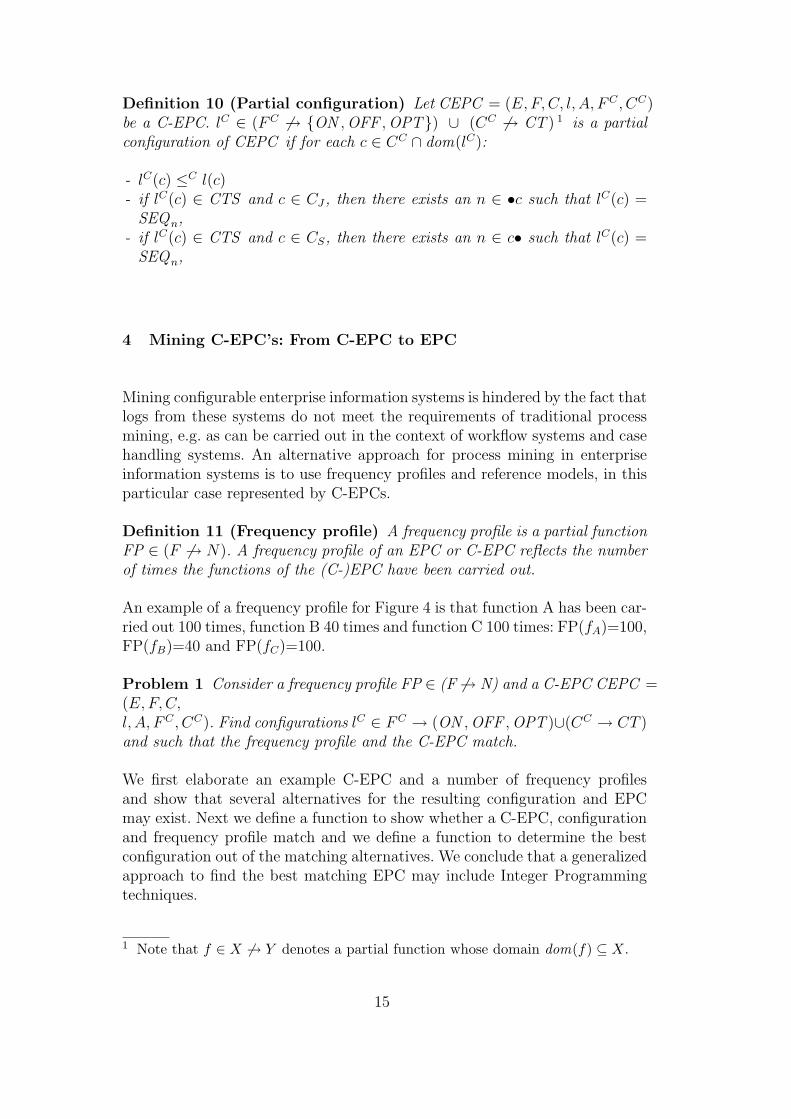
Definition 10 (Partial configuration) Let CEPC = (E,F,C, l, A, FC , CC)be a C-EPC. lC ∈ (FC 6→ {ON ,OFF ,OPT}) ∪ (CC 6→ CT ) 1 is a partialconfiguration of CEPC if for each c ∈ CC ∩ dom(lC):
- lC(c) ≤C l(c)- if lC(c) ∈ CTS and c ∈ CJ , then there exists an n ∈ •c such that lC(c) =
SEQn,- if lC(c) ∈ CTS and c ∈ CS, then there exists an n ∈ c• such that lC(c) =
SEQn,
4 Mining C-EPC’s: From C-EPC to EPC
Mining configurable enterprise information systems is hindered by the fact thatlogs from these systems do not meet the requirements of traditional processmining, e.g. as can be carried out in the context of workflow systems and casehandling systems. An alternative approach for process mining in enterpriseinformation systems is to use frequency profiles and reference models, in thisparticular case represented by C-EPCs.
Definition 11 (Frequency profile) A frequency profile is a partial functionFP ∈ (F 6→ N). A frequency profile of an EPC or C-EPC reflects the numberof times the functions of the (C-)EPC have been carried out.
An example of a frequency profile for Figure 4 is that function A has been car-ried out 100 times, function B 40 times and function C 100 times: FP(fA)=100,FP(fB)=40 and FP(fC)=100.
Problem 1 Consider a frequency profile FP ∈ (F 6→ N) and a C-EPC CEPC =(E, F, C,l, A, FC , CC). Find configurations lC ∈ FC → (ON ,OFF ,OPT )∪(CC → CT )and such that the frequency profile and the C-EPC match.
We first elaborate an example C-EPC and a number of frequency profilesand show that several alternatives for the resulting configuration and EPCmay exist. Next we define a function to show whether a C-EPC, configurationand frequency profile match and we define a function to determine the bestconfiguration out of the matching alternatives. We conclude that a generalizedapproach to find the best matching EPC may include Integer Programmingtechniques.
1 Note that f ∈ X 6→ Y denotes a partial function whose domain dom(f) ⊆ X.
15

4.1 Searching for configurations
An EPC consists of events, functions and connectors. A C-EPC may addition-ally contain configurable functions and three different types of configurableconnectors (&C , XORC and ORC). In this subsection we elaborate an ex-ample consisting of a C-EPC (with two configurable OR-connectors and oneconfigurable function as represented in Figure 7) and three frequency profiles,represented in Table 2.
c 1
c 2
c 3
c 4
B C
A
1
2
3
V
V
V
V
D
Fig. 7. Example of a configurable EPC
frequency frequency frequency
function profile A profile B profile C
A 100 100 100
B 0 100 80
C 100 100 60
D 0 100 70
Table 2Three frequency profiles for the C-EPC in Figure 7
Frequency profile A shows that in this particular case function D and theleftmost branch of the C-EPC have not been executed. Function D may havebeen configured OFF or OPT: lC ∈ {(D,OFF ), (D,OPT )}). In the lattercase, D has not been performed at runtime. The explanation why the leftmostbranch has not been executed is a bit more complex:
• during configuration time the configurable connectors c2 and c3 have been
16

configured SEQC , and at runtime function B could not be performed (EPCvariant 1 in Figure 8): lC = ((ORc2 , SEQC), (ORc3 , SEQC)) .
• during configuration time the configurable connectors c2 and c3 have beenconfigured XOR, and at runtime function B has not been performed (EPCvariant 2 in Figure 8): lC = ((ORc2 ,XOR), (ORc3 ,XOR)).
• during configuration time the configurable connectors c2 and c3 have beenconfigured OR, and at runtime function B has not been performed (EPCvariant 3 in Figure 8): lC = ((ORc2 ,OR), (ORc3 ,OR)).
c 1
c 4
C
A
(1)
V
V
c 1
c 2
c 3
c 4
B C
A
X
X
(2)
V
V
c 1
c 2
c 3
c 4
B C
A
V
V
(3)
V
V
Fig. 8. Alternative EPCs based on the C-EPC in Figure 7 and frequency profilesFP-A
Frequency profile B shows that functions A and D have been performed thesame number of times, which implies that function D should be configuredON or OPT: lC ∈ {(D,OFF ), (D,OPT )}). In the latter case, D has beenperformed each time at runtime. Furthermore, functions B and C have beenperformed the same number of times. This can be because:
• during configuration time the configurable connectors c2 and c3 have beenconfigured AND: lC = ((ORc2 , &), (ORc3 , &)).
• during configuration time the configurable connectors c2 and c3 have beenconfigured OR and coincidentally A, B and C have been performed the samenumber of times: lC = ((ORc2 ,OR), (ORc3 ,OR)).
Frequency profile C finally, does not leave any freedom for configuration. SinceD has been performed, but less than A, it should be configured OPT: lC =
17

(D,OPT ). Note that we assume that the log consists of complete cases withoutany noise which, in practice, is not necessarily the case. Furthermore, c2 andc3 can only be configured OR: lC = ((ORc2 ,OR), (ORc3 ,OR)).
From these examples, we conclude that deriving a configuration based on aC-EPC and a frequency profile is not unambiguous. The remainder of thissection is used to show when a particular configuration is allowed and if morethan one configuration is allowed, which configuration fits best.
4.2 Matching
Combining a particular C-EPC and frequency profile results in a configurationand related EPC. However, in general, this process may result in a number ofconfigurations and thus several different EPCs. In this subsection we definethe function match to show whether a C-EPC, configuration and frequencyprofile do match, in the next subsection we define a function to determine thebest configuration out of the matching alternatives.
A C-EPC can be considered a set of concrete EPCs; a particular EPC isdetermined by its configuration as defined in Definition 7. An EPC/C-EPC isa graph consisting of different nodes. Each node and each arc have a frequency.Through the frequency profile we only know the frequency of functions andnot of the other nodes. Assume that the frequency of each node n is givenby a variable xn and let fn be the frequency in the profile if n is a function.Consider the following system of equations: ∀n ∈ F : xn = fn and the setof equations generated by arcs. The exact formulation of the set of equationsis dependent on (i) the structure of the model, (ii) whether a function isconfigurable or not (and if applicable its configuration), and (iii) whether aconnector is configurable or not (and if applicable its configuration). For allnodes in the model, the applicable equations should be selected from the listbelow:
• Related to functions:· An arc ending in a function has a frequency that is equal to the frequency
of the arc starting from that function.· All arcs starting or ending in a non-configurable function or event have a
frequency that equals the frequency of that function or event.· All arcs starting or ending in a configurable function that has been con-
figured ON, have a frequency that equals the frequency of that function.· All arcs starting or ending in a configurable function that has been config-
ured OPT, have a frequency that is greater than or equal to the frequencyof that function.
· A configurable function that has been configured OFF, has a frequency 0.
18

• Related to AND-nodes (connectors or configurations):· An AND-node has a frequency that equals the frequency of each of the
arcs starting from that AND-node.· An AND-node has a frequency that is less than or equal to the frequency
of each of the arcs ending in that AND-node, and equals the frequency ofat least one of the arcs ending in that AND-node.
• Related to XOR-nodes (connectors or configurations):· A XOR-node has a frequency that equals the sum of the frequencies of all
arcs starting from that XOR-node.· A XOR-node has a frequency that equals the sum of the frequencies of all
arcs ending in that XOR-node.
• Related to OR-nodes (connectors or configurations)· An OR-node has a frequency that is less than or equal to the sum of the
frequencies of each of the arcs ending in that OR-node.· An OR-node has a frequency that is greater than or equal to the frequency
of each of the arcs ending in that OR-node.· An OR-node has a frequency that is less than or equal to the sum of the
frequencies of each of the arcs starting from that OR-node.· An OR-node has a frequency that is greater than or equal to the frequency
of each of the arcs starting from that OR-node.
• Related to SEQx-configurations (split)· A connector that has been configured SEQx, has a frequency that is equal
to the frequency of the arc starting from that connector and ending innode x.
· An arc starting from a connector that has been configured SEQx andending in any other node than x has a frequency 0.
· An arc starting from a connector that has been configured SEQx and end-ing in any node has a frequency equal to the frequency of that connector.
• Related to SEQx-configurations (join)· An arc starting from any node and ending in a connector that has been
configured SEQx has a frequency equal to the frequency of that connector.· A connector that has been configured SEQx, has a frequency that is equal
to the frequency of the arc starting from node x and ending in that con-nector.
· An arc ending in a connector that has been configured SEQx and startingfrom any other node than x has a frequency 0.
We have defined now a C-EPC and a frequency profile, and we are able todefine the set of equations that describe this situation. We are ready to definewhen a configuration matches with a C-EPC and a given frequency profile.
19
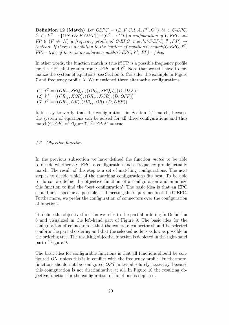
Definition 12 (Match) Let CEPC = (E, F, C, l, A, FC , CC) be a C-EPC,lC ∈ (FC → {ON, OFF, OPT})∪ (CC → CT ) a configuration of C-EPC andFP ∈ (F 6→ N) a frequency profile of C-EPC. match:(C-EPC, lC , FP ) →boolean. If there is a solution to the ‘system of equations’, match(C-EPC, lC,FP)= true; if there is no solution match(C-EPC, lC, FP)= false.
In other words, the function match is true iff FP is a possible frequency profilefor the EPC that results from C-EPC and lC . Note that we still have to for-malize the system of equations, see Section 5. Consider the example in Figure7 and frequency profile A. We mentioned three alternative configurations:
(1) lC = ((ORc2 , SEQC), (ORc3 , SEQC), (D,OFF ))(2) lC = ((ORc2 ,XOR), (ORc3 ,XOR), (D,OFF ))(3) lC = ((ORc2 ,OR), (ORc3 ,OR), (D,OFF ))
It is easy to verify that the configurations in Section 4.1 match, becausethe system of equations can be solved for all three configurations and thusmatch(C-EPC of Figure 7, lC , FP-A) = true.
4.3 Objective function
In the previous subsection we have defined the function match to be ableto decide whether a C-EPC, a configuration and a frequency profile actuallymatch. The result of this step is a set of matching configurations. The nextstep is to decide which of the matching configurations fits best. To be ableto do so, we define the objective function of a configuration and minimizethis function to find the ‘best configuration’. The basic idea is that an EPCshould be as specific as possible, still meeting the requirements of the C-EPC.Furthermore, we prefer the configuration of connectors over the configurationof functions.
To define the objective function we refer to the partial ordering in Definition6 and visualized in the left-hand part of Figure 9. The basic idea for theconfiguration of connectors is that the concrete connector should be selectedconform the partial ordering and that the selected node is as low as possible inthe ordering tree. The resulting objective function is depicted in the right-handpart of Figure 9.
The basic idea for configurable functions is that all functions should be con-figured ON, unless this is in conflict with the frequency profile. Furthermore,functions should not be configured OPT unless absolutely necessary, becausethis configuration is not discriminative at all. In Figure 10 the resulting ob-jective function for the configuration of functions is depicted.
20

0
OR
AND XOR
SEQ 2
2
1
0
OR
AND XOR
SEQ 1 SEQ
2 SEQ 1
1
Fig. 9. Objective function for the configuration of connectors
OPT
ON OFF
100
1 0
Fig. 10. Objective function for the configuration of functions
The objective function can now be formulated as: minimize the sum of theobjective function due to the configuration of all configurable connectors andthe objective function due to the configuration of all configurable functions.
For the example in subsection 4.1 we conclude that variant 1 (both connectorsconfigured SEQC) and function D configured OFF is the best configuration,see Table 5.
lC lC(c2) lC(c3) lC(D) Objective function
1 SEQC SEQC OFF ⇒ 0+0+1=1
2 XOR XOR OFF ⇒ 1+1+1=3
3 OR OR OFF ⇒ 2+2+1=5
Table 3Configurations for the C-EPC in Figure 7 and frequency profile FP-A
4.4 Conclusion
In this section we have defined the function match to be able to decide whethera C-EPC, a configuration and a frequency profile actually match. The result ofthis step is a set of matching configurations. The next step is to decide whichof the matching configurations fits best. To be able to do so, we defined theobjective function for a configuration. Summarizing, if we want to determinean EPC based on a C-EPC and a frequency profile, we go through the followingsteps:
21

(1) find all matching configurations(2) minimize the objective function
The approach that we followed in Section 4.2 (find all solutions of a system ofequations) and Section 4.3 (minimize a particular objective function) can beperformed in one step by making use of Integer Programming techniques. Thishas an additional advantage since standard software for solving Integer Pro-gramming problems is generally available. In the next section we reformulatethe above described approach in such a way that integer programming can beapplied. Subsequently we will discuss the required variables, the constraintsand the objective function.
5 Formulating the Integer Programming problem
Let CEPC = (E, F, C, l, FC , CC) be a C-EPC and FP ∈ (F 6→ N) be a fre-quency profile. A (C-)EPC is a graph consisting of different nodes. Each nodeand each arc have a frequency. The frequency profile records the frequency offunctions and not of the other node types 2 . Consider the following IntegerProgramming problem.
5.1 Variables
We consider two types of variables: variables to describe the model elementsand variables to describe the configuration settings, which are our decisionvariables. These decision variables are related to the configuration of functionsand the configuration of connectors.
All elements in the C-EPC have a frequency.
∀x ∈ E ∪ F ∪ C ∪ A : freqx ∈ N (1)
2 We assume that the EPCs are sound, i.e. meet the following three requirements: (i)for each case that is represented in the start event, one and only one representationexists (eventually) in the end event, (ii) when the representation of a case appearsin the end event, there is no other representation of this case present in the EPC,and (iii) for each function in the EPC it is possible to move from the start eventto a situation in which this function can be executed. Furthermore we assume thatthe frequency profiles represent complete cases, i.e. the frequency profile does notcontain any noise.
22

A configurable function can be configured ON, OFF or OPT.
∀f ∈ FC : conf f ∈ {ON ,OFF ,OPT} (2)
All configurable connectors can be mapped onto a concrete connector withinCT, provided that the concrete connector is more specific than the configurableconnector (cf. partial ordering in Definition 6). Moreover, if lC(c) = SEQn,then n should be in the preset (for join connectors) or in the postset (for splitconnectors).
∀c ∈ CC : conf c ∈ {x ∈ CT |x ≤C l(c) ∧ (3)
if lC(c) ∈ CTS and c ∈ CJ , there exists an n ∈ •c such that x = SEQn ∧if lC(c) ∈ CTS and c ∈ CS, there exists an n ∈ c • such that x = SEQn}
5.2 Constraints
We consider several groups of constraints: constraints related to functions,constraints related to concrete, non-configurable connectors (AND, OR andXOR) and to configurable nodes that have been configured (SEQ-, AND-, OR-or XOR-configurations).
5.2.1 Constraints related to functions
All configurable and non-configurable functions have a frequency as recordedin the frequency profile FP.
∀f ∈ dom(FP) : freqf = FP(f) (4)
An arc ending in a function has a frequency that is equal to the frequency ofthe arc starting from that function.
∀f ∈ F ∀(x1, y1), (x2, y2) ∈ A, (y1 = x2 = f) : freq (x1,y1) = freq (x2,y2) (5)
f (x
1 ,y
1 ) (x
2, y
2 )
Fig. 11. Illustration of equation 5
23

All arcs starting or ending in a non-configurable function or event have afrequency that equals the frequency of that function or event.
∀x ∈ (F\FC) ∪ E ∀(y, z) ∈ A, x ∈ {y, z} : freq (y,z) = freqx (6)
x (y,z)
x (y,z )
Fig. 12. Two illustrations of equation 6
All arcs starting or ending in a configurable function that has been configuredON, have a frequency that equals the frequency of that function.
∀f ∈ FC ∀(x, y) ∈ A, f ∈ {x, y} : conf f = ON ⇒ freq (x,y) = freqf (7)
All arcs starting or ending in a configurable function that has been configuredOPT, have a frequency that is greater than or equal to the frequency of thatfunction.
∀f ∈ FC ∀(x, y) ∈ A, f ∈ {x, y} : conf f = OPT ⇒ freq (x,y) ≥ freqf (8)
A configurable function that has been configured OFF, has a frequency 0.
∀f ∈ FC : conf f = OFF ⇒ freqf = 0 (9)
f (x,y )
f (x,y )
Fig. 13. Two illustrations of equations 7, 8 and 9
5.2.2 Constraints related to concrete AND-connectors
A non-configurable AND-connector has a frequency that equals the frequencyof each of the arcs starting from that AND-connector.
∀c ∈ C\CC , l(c) = & ∀(x, y) ∈ A, x = c : freq (x,y) = freqc (10)
A non-configurable AND-connector has a frequency that is less than or equalto the frequency of each of the arcs ending in that AND-connector, and equalsthe frequency of at least one of the arcs ending in that AND-connector.
∀c ∈ C\CC , l(c) = & ∀(x, y) ∈ A, y = c : freq (x,y) ≥ freqc (11)
∀c ∈ C\CC , l(c) = & ∃(x, y) ∈ A, y = c : freq (x,y) = freqc (12)
24

(x ,y )
V
c
(x ,y )
V
c
Fig. 14. Illustrations of equation 10 (left) and equations 11 and 12 (right)
5.2.3 Constraints related to concrete XOR-connectors
A non-configurable XOR-connector has a frequency that equals the sum ofthe frequencies of all arcs starting from that XOR-connector.
∀c ∈ C\CC , l(c) = XOR :∑
(x,y)∈Ax=c
freq (x,y) = freqc (13)
A non-configurable XOR-connector has a frequency that equals the sum ofthe frequencies of all arcs ending in that XOR-connector.
∀c ∈ {C\CC |l(c) = XOR} :∑
(x,y)∈Ay=c
freq (x,y) = freqc (14)
c
(x ,y )
X
(x ,y )
X
c
Fig. 15. Illustrations of equation 13 (left) and equation 14 (right)
5.2.4 Constraints related to concrete OR-connectors
A non-configurable OR connector has a frequency that is less than or equal tothe sum of the frequencies of each of the arcs ending in, respectively startingfrom that OR-connector.
∀c ∈ C\CC , l(c) = OR :∑
(x,y)∈Ac∈{x,y}
freq (x,y) ≥ freqc (15)
A non-configurable OR-connector has a frequency that is greater than or equalto the frequency of each of the arcs ending in, respectively starting from thatOR-connector.
∀c ∈ C\CC , l(c) = OR ∀(x, y) ∈ A, c ∈ {x, y} : freq (x,y) ≤ freqc (16)
25

(x ,y )
V
c
(x ,y )
V
c
Fig. 16. Illustrations of equations 15 and 16
5.2.5 Constraints related to SEQx-configurations
A connector that has been configured SEQx, has a frequency that is equal tothe frequency of the arc starting from that connector and ending in node x.
∀c ∈ CC , x ∈ E ∪ F ∪ C, (c, x) ∈ A : conf c = SEQx ⇒ freq (c,x) = freqc(17)
An arc starting from a connector that has been configured SEQx and endingin any other node than x has a frequency 0.
∀c ∈ CC , x ∈ E ∪ F ∪ C, (c, x) ∈ A ∀y ∈ c•, y 6= x : (18)
conf c = SEQx ⇒ freq (c,y) = 0
An arc starting from any node and ending in a connector that has been con-figured SEQx has a frequency equal to the frequency of that connector.
∀c ∈ CC , x ∈ E ∪ F ∪ C, (c, x) ∈ A ∀z ∈ •c : (19)
conf c = SEQx ⇒ freq (z,c) = freqc
A connector that has been configured SEQx, has a frequency that is equal tothe frequency of the arc starting from node x and ending in that connector.
∀c ∈ CC , x ∈ E ∪ F ∪ C, (x, c) ∈ A : conf c = SEQx ⇒ freq (x,c) = freqc(20)
An arc ending in a connector that has been configured SEQx and startingfrom any other node than x has a frequency 0.
∀c ∈ CC , x ∈ E ∪ F ∪ C, (x, c) ∈ A ∀y ∈ •c, y 6= x : (21)
conf c = SEQx ⇒ freq (y,c) = 0
An arc starting from a connector that has been configured SEQx and endingin any node has a frequency equal to the frequency of that connector.
26

∀c ∈ CC , x ∈ E ∪ F ∪ C, (x, c) ∈ A ∀z ∈ c• : (22)
conf c = SEQx ⇒ freq (c,z) = freqc
(c,x )
?
(c,y )
conf c =SEQ
x
(z,c) (x,c )
?
(y,c )
conf c =SEQ
x
(c,z)
Fig. 17. Illustrations of equations 17, 18 and 19 (left) and equations 20, 21 and 22(right)
5.2.6 Constraints related to AND-configurations
Consider a configurable connector. If this connector has been configured aconcrete AND, this connector has a frequency that equals the frequency ofeach of the arcs starting from that connector.
∀c ∈ CC , (x, y) ∈ A, x = c : conf c = AND ⇒ freq (x,y) = freqc (23)
Consider a configurable connector. If this connector has been configured aconcrete AND, this connector has a frequency that less than or equal to thefrequency of each of the arcs ending in that connector.
∀c ∈ CC , (x, y) ∈ A, y = c : conf c = AND ⇒ freq (x,y) ≥ freqc (24)
∀c ∈ CC ∃(x, y) ∈ A, y = c : confc = & ⇒ freq (x,y) = freqc (25)
(x ,y )
? conf c =AND
(x ,y )
? conf c =AND
c c
Fig. 18. Illustrations of equation 23 (left) and equations 24 and 25 (right)
5.2.7 Constraints related to XOR-configurations
Consider a configurable connector. If this connector has been configured aconcrete XOR, this connector has a frequency that equals the sum of thefrequencies of each of the arcs starting from that connector.
∀c ∈ CC : conf c = XOR ⇒ ∑(x,y)∈A
x=c
freq (x,y) = freqc (26)
27

Consider a configurable connector. If this connector has been configured aconcrete XOR, this connector has a frequency that equals the sum of thefrequencies of each of the arcs ending in that connector.
∀c ∈ CC : conf c = XOR ⇒ ∑(x,y)∈A
y=c
freq (x,y) = freqc (27)
(x ,y )
? conf c =XOR
c
(x ,y )
? conf c =XOR
c
Fig. 19. Illustrations of equation 26 (left) and equation 27 (right)
5.2.8 Constraints related to OR-configurations
Consider a configurable connector. If this connector has been configured aconcrete OR, this connector has a frequency that is less than or equal to thesum of the frequencies of each of the arcs ending in , respectively starting fromthat connector.
∀c ∈ CC : conf c = OR ⇒ ∑(x,y)∈Ac∈{x,y}
freq (x,y) ≥ freqc (28)
Consider a configurable connector. If this connector has been configured aconcrete OR, this connector has a frequency that is greater than or equal tothe frequency of each of the arcs ending in , respectively starting from thatconnector.
∀c ∈ CC , (x, y) ∈ A, c ∈ {x, y} : conf c = OR ⇒ freq (x,y) ≤ freqc (29)
(x ,y )
? l(c)=OR
(x ,y )
? conf c =OR
c c
Fig. 20. Illustrations of equations 28 and 29
5.3 Objective function
Up to now, we have formulated the system variables and the decision variables,which enabled us to formulate the constraints of our Integer Programmingproblem. In this subsection, we define the objective function.
28
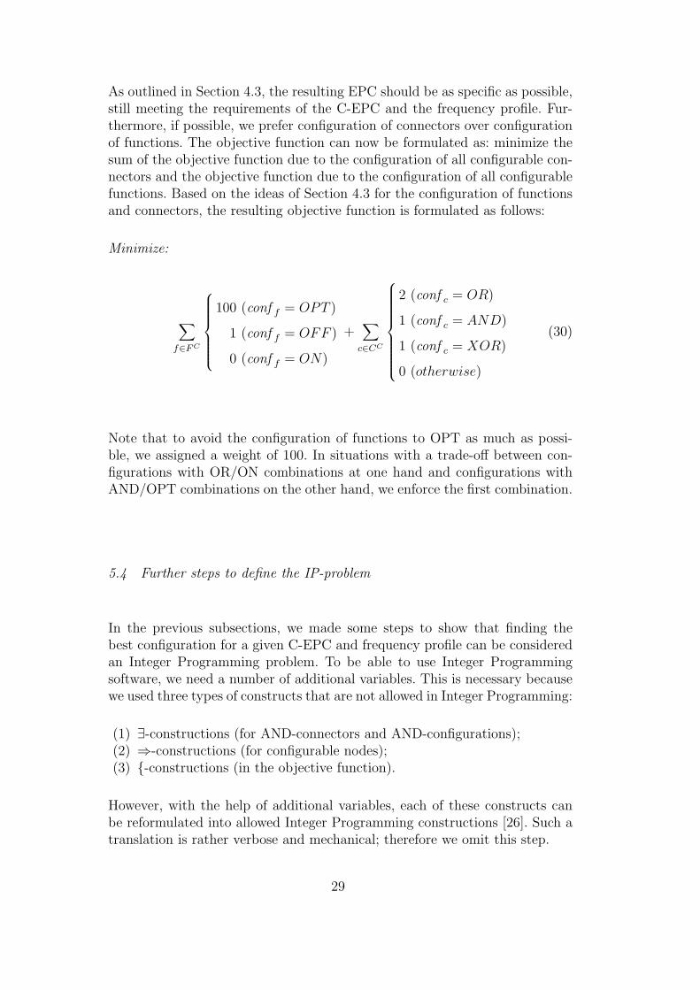
As outlined in Section 4.3, the resulting EPC should be as specific as possible,still meeting the requirements of the C-EPC and the frequency profile. Fur-thermore, if possible, we prefer configuration of connectors over configurationof functions. The objective function can now be formulated as: minimize thesum of the objective function due to the configuration of all configurable con-nectors and the objective function due to the configuration of all configurablefunctions. Based on the ideas of Section 4.3 for the configuration of functionsand connectors, the resulting objective function is formulated as follows:
Minimize:
∑
f∈F C
100 (conf f = OPT )
1 (conf f = OFF )
0 (conf f = ON)
+∑
c∈CC
2 (conf c = OR)
1 (conf c = AND)
1 (conf c = XOR)
0 (otherwise)
(30)
Note that to avoid the configuration of functions to OPT as much as possi-ble, we assigned a weight of 100. In situations with a trade-off between con-figurations with OR/ON combinations at one hand and configurations withAND/OPT combinations on the other hand, we enforce the first combination.
5.4 Further steps to define the IP-problem
In the previous subsections, we made some steps to show that finding thebest configuration for a given C-EPC and frequency profile can be consideredan Integer Programming problem. To be able to use Integer Programmingsoftware, we need a number of additional variables. This is necessary becausewe used three types of constructs that are not allowed in Integer Programming:
(1) ∃-constructions (for AND-connectors and AND-configurations);(2) ⇒-constructions (for configurable nodes);(3) {-constructions (in the objective function).
However, with the help of additional variables, each of these constructs canbe reformulated into allowed Integer Programming constructions [26]. Such atranslation is rather verbose and mechanical; therefore we omit this step.
29

5.5 Example
In the previous subsections we formulated the derivation of a configurationbased on a C-EPC and frequency profile in such a way that it can be con-sidered an Integer Programming problem. In this subsection, we show thisapproach for a concrete example. Consider the C-EPC shown in Figure 7 andfrequency profile FP(fA) = 100, FP(fB) = 40, FP(fC) = 60 and FP (fD =80). The C-EPC consists of three functions, of which f3 is configurable, and of4 connectors, of which c2 and c3 are configurable. The corresponding IntegerProgramming problem is defined as follows (for explanation of the variablesand constraints in this example, see appendix A).
min∑
f∈F C
100 (conf f = OPT )
1 (conf f = OFF )
0 (conf f = ON )
+∑
c∈CC
2 (conf c = OR)
1 (conf c = &)
1 (conf c = XOR)
0 (otherwise)
s.t. freqfA= FP(fA) = 100
freqfB= FP(fB) = 40
freqfC= FP(fC) = 60
freqfD= FP(fD) = 80
freq (e0,fA) = freq (fA,e1)
freq (c2,fB) = freq (fB ,c3)
freq (c2,fC) = freq (fC ,c3)
freq (c1,fD) = freq (fD,c4)
freqe0= freq (e0,fA)
freq (e0,fA) = freqfA
freqfA= freq (fA,e1)
freq (fA,e1) = freqe1
freqe1= freq (e1,c1)
freq (c2,fB) = freqfB
freqfB= freq (fB ,c3)
freq (c2,fC) = freqfC
freqfC= freq (fC ,c3)
freq (c4,e2) = freqe2)
conf fD= OFF ⇒ freqfD
= 0
conf fD= OPT ⇒ freqfD
≤ freq (c1,fD)
conf fD= OPT ⇒ freqfD
≤ freq (fD,c4)
30

conf fD= ON ⇒ freqfD
= freq (c1,fD)
conf fD= ON ⇒ freqfD
= freq (fD,c4)
freqc1 = freq (c1,c2)
freqc1 = freq (c1,fD)
freq (fD,c4) ≥ freqc4 ∧ freq (c3,c4) = freqc4
freq (c3,c4) = freqc4 ∨ freq (fD,c4) = freqc4
conf c2 = SEQfB⇒ freq (c2,fB) = freqc2
conf c2 = SEQfC⇒ freq (c2,fC) = freqc2
conf c2 = SEQfB⇒ freq (c2,fC) = 0
conf c2 = SEQfC⇒ freq (c2,fB) = 0
conf c2 = SEQfB⇒ freq (c1,c2) = freq (c2,fB)
conf c2 = SEQfC⇒ freq (c1,c2) = freq (c2,fC)
conf c3 = SEQfB⇒ freq (fB ,c3) = freqc3
conf c3 = SEQfC⇒ freq (fC ,c3) = freqc3
conf c3 = SEQfB⇒ freq (fC ,c3) = 0
conf c3 = SEQfC⇒ freq (fB ,c3) = 0
conf c3 = SEQfB⇒ freq (fB ,c3) = freq (c3,c4)
conf c3 = SEQfC⇒ freq (fC ,c3) = freq (c3,c4)
conf c2 = & ⇒ freq (c2,fB) = freqc2 ∧ freq (c2,fC) = freqc2
conf c3 = & ⇒ freq (fB ,c3) ≥ freqc3 ∧ freq (fC ,c3) ≥ freqc3
conf c3 = & ⇒ freq (fB ,c3) = freqc3 ∨ freq (fC ,c3) = freqc3
conf c2 = XOR ⇒ freq (c2,fB) + freq (c2,fC) = freqc2
conf c3 = XOR ⇒ freq (fB ,c3) + freq (fC ,c3) = freqc3
conf c2 = OR ⇒ freq (c2,fB) + freq (c2,fC) ≥ freqc2
conf c3 = OR ⇒ freq (fB ,c3) + freq (fC ,c3) ≥ freqc3
conf c2 = OR ⇒ freq (c2,fB) ≤ freqc2 ∧ freq (c2,fC) ≤ freqc2
conf c3 = OR ⇒ freq (fB ,c3) ≤ freqc3 ∧ freq (fC ,c3) ≤ freqc3
In this example, the solution of the system of equations is conf fD= OPT ,
conf c2 ∈ {OR,XOR} and conf c3 ∈ {OR,XOR}. It is easy to verify thatconffD
= OPT , confc2 = XOR and confc3 = XOR is the solution of thisInteger Programming problem.
31

6 Mining C-EPCs: From EPC-Max to C-EPC
Up to now, we assumed that a reference model represented by a C-EPC wasavailable, and from a conceptual viewpoint reference models of configurable en-terprise information systems should indeed be configurable. In practice, thesemodels are not configurable yet and can be characterized as upper bound ormaximal process models. The second step in our research takes this traditionalreference model, an EPC-Max, as a starting point. Additionally we have oneparticular log, i.e. a frequency profile that shows the frequency that particularprocess steps have been executed. This process results in a configurable EPCand a configuration that fits the log (see Section 6.1). It is evident that theresulting C-EPC and configuration depend on this only log and probably aredifferent when based on another log or multiple logs. This step is elaboratedin Section 6.2.
6.1 Deriving ‘a’ C-EPC
Although the application of non-configurable reference models is current prac-tice, this is not an ideal situation. When mining process models from config-urable enterprise information systems the concept of configurable referencemodels supports mining the actual processes. Additionally, the derived con-figurable reference model is a useful spin-off.
Problem 2 Consider a frequency profile FP ∈ (F 6→ N) and an EPC EPC=(E,F,C,l,A). Find a C-EPC CEPC = (E, F, C, l, A, FC , CC) and a configura-tion lC ∈ (FC → ON ,OFF ,OPT ) ∪ (CC → CT ) such that the frequencyprofile, the C-EPC and the configuration match.
6.1.1 Approach
When mining a process model from an EPC-Max, we start to find the C-EPC. We will demonstrate that the approach developed in Section 4 is alsoapplicable for this type of process mining.
We first define the term flexible EPC, this is a C-EPC that resembles theEPC completely, however, all concrete connectors are mapped onto their con-figurable counterparts and all functions are changed into configurable ones.
Definition 13 (flexible EPC) Let EPC=(E,F,C,l,A). Then flex(EPC) =(E ′, F ′, C ′, l′, A′,FC , CC) with E ′ = E,F ′ = F,C ′ = C, l′ = l, A′ = A,FC = F, CC = C.
32

We use flexible EPCs as an intermediary result for our mining approach. Re-call that this approach included two steps: the matching function and theobjective function. The function match is used to decide whether a particularconfiguration, C-EPC (in this case flex(EPC)) and frequency profile matchand the objective function to decide for all matching configurations whichconfiguration fits best.
6.1.2 Example
Consider the EPC in Figure 4, a simple EPC-Max containing a XOR con-nector. In Table 4 two frequency profiles for this EPC is shown. Frequencyprofile A is a log of an enterprise that only manufactured product B, whereasfrequency profile B is a log of an enterprise that manufactured both productB and C, but not in the same production order.
frequency frequency
function profile A profile B
A 100 140
B 100 100
C 0 40
D 100 140
Table 4Two frequency profiles for the C-EPC in Figure 4
The first step is transform this EPC-Max (left-hand side of Figure 21) into aflexible EPC (right-hand side of Figure 21).
The second step is to find all matching configurations. With reference to Def-inition 6, the XORC-connector can be configured XOR, or SEQ. Since wedeparted from a XOR-connector in the EPC-Max, at this point we choose tostick to lC(c1) = (XOR, XOR) and lC(c2) = (XOR, XOR) and we come backon this in the next subsection.
With respect to the functions, we see the following alternatives:
• For frequency profile A, functions A, B and D can be non-configurable, andif configurable these may be configured ON or OPT. Function C may alsobe configured OFF.
• For frequency profile B, all functions can be non-configurable, and if con-figurable these may be configured ON or OPT.
It is easy to verify that match(flex(EPC),lC ,FP-A) = true for the configura-tions in Table 5.
33

flexible EPC concrete EPC
1
A
2
X
C B
5
3
6
X
4
D
1
A
2
X
C B
5
3
6
X
4
D
Fig. 21. From EPC to flexible C-EPC
The third step is to calculate the objective function. The results for frequencyprofile A are summarized in the rightmost column of Table 5, for frequencyprofile B this can be done in the same way. For both frequency profiles wesee that the (XOR,XOR) configuration with all functions configured ON fitsbest.
Our last step in deriving a definitive C-EPC is to consider whether config-urable nodes should remain configurable; i.e. configurable functions that arealways ON become normal functions and connectors that are mapped ontotheir identity connector become concrete connectors. All other nodes need tobe configurable. Since only one frequency profile is available, after this stepindeed no configurable connectors exist.
6.1.3 Further restriction of the C-EPC
The above outlined approach is applicable for decisions that are made atruntime, or at least for frequency profiles from which we cannot conclude thata decision is made at runtime or at configuration time. However, there is animportant class of frequency profiles that shows that the decision appears tobe made at configuration time. In case a frequency profile is (co-incidently?)more specific than the concrete connector in the EPC-max required (in ourexample in case of frequency profile A), it is possible to further restrict theflex(EPC) to determine a C-EPC, while still preserving the match condition.This si called ’overfitting’. This step introduces two questions: (1) what is the
34

lC lC(A) lC(c1) lC(B) lC(C) lC(c2) lC(D) Objective function
1 ON XOR ON ON XOR ON 0+1+0+0+1+0=2
2 ON XOR ON ON XOR OPT 0+1+0+0+1+100=102
3 ON XOR ON OPT XOR ON 0+1+0+100+1+0=102
4 ON XOR ON OPT XOR OPT 0+1+0+100+1+100=202
5 ON XOR ON OFF XOR ON 0+1+0+1+1+0=3
6 ON XOR ON OFF XOR OPT 0+1+0+1+1+100=103
7 ON XOR OPT ON XOR ON 0+1+100+0+1+0=102
8 ON XOR OPT ON XOR OPT 0+1+100+0+1+100=202
9 ON XOR OPT OPT XOR ON 0+1+100+100+1+0=202
10 ON XOR OPT OPT XOR OPT 0+1+100+100+1+100=302
11 ON XOR OPT OFF XOR ON 0+1+100+1+1+0=103
12 ON XOR OPT OFF XOR OPT 0+1+100+1+1+100=203
13 OPT XOR ON ON XOR ON 0+1+0+0+1+0=102
14 OPT XOR ON ON XOR OPT 0+1+0+0+1+100=202
15 OPT XOR ON OPT XOR ON 0+1+0+100+1+0=202
16 OPT XOR ON OPT XOR OPT 0+1+0+100+1+100=302
17 OPT XOR ON OFF XOR ON 0+1+0+1+1+0=103
18 OPT XOR ON OFF XOR OPT 0+1+0+1+1+100=203
19 OPT XOR OPT ON XOR ON 0+1+100+0+1+0=202
20 OPT XOR OPT ON XOR OPT 0+1+100+0+1+100=302
21 OPT XOR OPT OPT XOR ON 0+1+100+100+1+0=302
22 OPT XOR OPT OPT XOR OPT 0+1+100+100+1+100=402
23 OPT XOR OPT OFF XOR ON 0+1+100+1+1+0=203
24 OPT XOR OPT OFF XOR OPT 0+1+100+1+1+100=303
Table 5Configurations for the flex(EPC) in Figure 21 and frequency profile FP-A
scope of the EPC-max, the reference model we started from, and (2) what isde scope of the C-EPC, the reference model that we are deriving. The answeron the first question can very well be a broad scope, e.g., all organizations thatmight use SAP R/3. The answer on the second question very much dependson the scope of our modelling domain, e.g. a particular branch of industry
35

or only all business units in our company. It is clear that this step requiresadditional information and cannot be performed automatically.
If we decide to allow further restrictions as described above, we have to payspecial attention to (partial) C-EPCs that might include SEQn solutions, be-cause SEQn is merely a configuration setting instead of a connector type.Basically we have three alternatives:
• The node remains configurable (XORC) and the configuration setting isSEQn;
• Although SEQn is a configuration instead of a connector type, we admitconcrete SEQn connectors;
• If possible, the connector is removed and the graph structure might change.
We use alternative 1 in our approach, because alternative 2 introduces a newnode type which is not necessary and alternative 3 complicates the derivationof C-EPCs based on multiple logs. Consequently, this approach may result inone configurable connector (XORC) which is configured SEQn.
6.1.4 Summary
If we want to determine a C-EPC and configuration based on an EPC-maxand a frequency profile, we go through the following steps:
(1) transform the EPC-max into a flexible C-EPC(2) find all matching configurations(3) minimize the objective function(4) restrict the resulting C-EPC if possible
6.2 From EPC-Max to ‘the’ C-EPC
The mining process can very well be based on a single log; in practice, how-ever, also a number of logs may be available. These logs may come from thesame company but covering another period of time, or these may come fromother business units or even from competing businesses. The scope of the con-figurable reference model being developed is dependent on the origin of theset of logs. In case of multiple logs of one particular company, the accuracy ofthe reference model will increase, in case of multiple logs of competitors, thescope of the reference model will be enlarged.
Problem 3 Consider a set of frequency profiles FP1 ∈ (F 6→ N) – FPn ∈(F 6→ N) and an EPC EPC=(E,F,C,l,A). Find a C-EPC CEPC = (E, F, C, l,A, FC , CC) and a configuration lC ∈ (FC → ON ,OFF ,OPT ) ∪ (CC → CT )
36

such that the frequency profiles, the C-EPC and the configurations match.
The third step in our research also takes the traditional reference model, anEPC-Max, as a starting point. Additionally we have a set of logs, i.e. frequencyprofiles. This process results in a configurable EPC and a configuration thatfits all logs. It is evident that the resulting EPC and configuration dependon this set of logs. Although it is more likely to be the correct C-EPC thanwhen based on one particular log, the result may be different when based onanother class of logs. For example, the set of logs may originate from a numberof business units within an enterprise, but also from a number of enterpriseswithin a particular industry sector (e.g. utilities, automotive, etc.) or acrossindustry sectors.
6.2.1 Searching for the C-EPC
Starting from an EPC-Max containing a (concrete) XOR connector and twologs (frequency profiles), we are constructing a C-EPC that fits both logs.Consider the EPC of Figure ?? and frequency profiles A and B in Table ??.In Section ?? we have shown that FP-A results in the C-EPC at the left partof Figure 22 and for FP-B at the middle part of Figure 22. Intuitively thisresults in a combined C-EPC that is shown at the right part of Figure 22.
EPC based
on FP-A
EPC based
on FP-B
EPC based on
FP-A and FP-B
XOR C ->
SEQe 2
e 1
f A
e 2
XOR
f C
f B
e 5
e 3
e 6
XOR
e 4
XOR C ->
SEQe 4 f
D
XOR C ->
SEQe 3
e 1
f A
e 2
XOR
f C
f B
e 5
e 3
e 6
XOR
e 4
XOR C ->
SEQe 5 f
D
e 1
f A
e 2
XOR
f C
f B
e 5
e 3
e 6
XOR
e 4
f D
Fig. 22. Aggregation of C-EPCs
37

6.2.2 Approach to derive ‘the’ C-EPC
To derive a C-EPC that fits n logs, we use the approach for 1 log (see Section6.1) and apply this n times. The result is a set of C-EPCs that can be analyzedwith respect to differences in configuration settings. In case of a difference be-tween two C-EPCs, the least common multiple is chosen. Again we start withconnectors, and within the configuration of connectors we configure the func-tions. Note that we assume that the C-EPCs have the same graph structure.The least common multiple for two connectors is based on the idea it should beas specific as possible on the one hand, and cover the scope of both connectorson the other hand. For example, for two OR-nodes this results in a new OR-node; a XOR-node and a SEQ-node result in a XORC-node, and an &-nodeand a XOR-node result in a ORC-node. The least common multiple for func-tions is defined the same way. If two functions have the same configurations,the common multiple is equal to this. If the configuration of two functions isdifferent, the least common multiple is F with lC(F ) ∈ {ON ,OPT ,OFF}.The least common multiple for connectors and functions is depicted in Figure23.
OR C
AND C XOR C
OR XOR AND
F
F
l c =OFF
F F
l c =OPT
Fig. 23. Least common multiple for connectors and functions
6.2.3 Summary
Summarizing, if we want to determine a C-EPC based on an EPC and nfrequency profiles FP1-FPn, we apply the approach for one log n times, andmerge the results by calculating the least common multiple for the resultingC-EPCs and configurations. This results in the following approach:
(1) transform the EPC in a flexible C-EPC(2) for each FP:
• find all matching configurations• minimize the objective function• restrict the resulting C-EPC
(3) determine the least common multiple for the set of C-EPCs
38

7 Related work
The work described in this paper has been inspired by process mining fromevent logs [5,6,9,15–18,24,25,36–38,42–44]. The basic idea was to test the pro-cess mining techniques developed in workflow and case-handling environmentsin a more general enterprise information systems environment. We found thatin general not all requirements for process mining were met, i.e. (i) each eventrefers to an activity, (ii) each event refers to a case, and (iii) events are to-tally ordered. Apart from process mining tools and techniques, we consideredSocial Network Analysis [8] and its implications for mining Social Networksfrom event logs [4]. This approach is based on the same requirements as pro-cess mining, and additionally requires that each event refers to a performer.For the same reasons, this approach is a good source for inspiration, but inits current form not generally applicable for mining enterprise informationsystems.
We have high expectations of mining enterprise information systems from abusiness perspective since it may contribute to (re)configuration and upgradesof such systems at one hand, and it allows for process performance analysison the other hand.
In the area of (re)configuration and upgrading of enterprise information sys-tems, a lot of work has been done with respect to reference models in general[10] and related to particular enterprise information systems [13,41]. Further-more, we already addressed the requirements to have more intuitive, exe-cutable and configurable business process models as described in [27,31,32].Such reference models are very helpful to mine Enteprise Systems in case eventlogs as described before are not available.
In the area of performance analysis, two types of analysis should be distin-guished: analysis based on descriptive models and analysis based on how pro-cesses are actually executed. Analysis based on descriptive models can bedone, e.g., by making use of mathematical models or simulation models. How-ever, any approach based on descriptive models lack sufficient feedback fromreal life. On the latter subject we already discussed two tools: Reverse Busi-ness Engineer [34,28] and ARIS Process Performance Manager [19]. Both toolshave limitations with respect to process mining: these tools still require processknowledge prior to application of the tool, whereas our approach only requiresexistence of standard reference models. To the knowledge of the authors, noacademic publications in this area are available yet.
39

8 Conclusions and further research
8.1 Conclusions
This paper proposes a solution for process mining from incomplete system logs.Existing mining approaches can be applied when an event log is composed ofat least a combination of case-ids and task-ids. In this paper, we discussedhow process mining can be applied if this combination of case-ids and task-idsis not available.
The approach that we followed is based on the frequency that a particulartransaction has been executed, recorded in a frequency log. Additionally wemake use of existing reference models, especially Event-driven Process Chains(EPCs) and the configurable couterpart (C-EPCs).
First we elaborated the idea to derive a configuration of the reference modelbased on a C-EPC and a frequency profile. To be able to do so, we defined thefunction match to decide whether a C-EPC, a configuration and a frequencyprofile match, and we defined the objective function to decide which of thematching configurations fits best.
In the approach to decide whether C-EPC, configuration and frequency profilematch, the (C)-EPC is considered to be a graph consisting of different nodes;each node and each arc have a frequency. Subsequently we consider a systemof equations generated by the arcs, making use of the characteristics of nodes(e.g. ‘an arc ending in a function has a frequency that is equal to the frequencyof the arc starting from that function’ or ‘a XOR-node has a frequency thatequals the sum of the frequencies of all arcs staring from that XOR-node’).
The function match can be applied on the (finite) set of possible configura-tions and results in the set of configurations that match with the particularfrequency profile. The objective function yields the configuration that matchesthe frequency profile best.
The approach that we followed (find all solutions of a system of equations andthen minimize a particular objective function) can be performed in one stepby making use of Integer Programming techniques. This has an additionaladvantage since standard software for solving Integer Programming problemsis generally available.
From a conceptual viewpoint reference models of configurable enterprise in-formation systems should be configurable. In practice, these models are notconfigurable yet and can be characterized as upper bound or maximal process
40

model. Therefore, the second step in our research takes a frequency profile anda traditional reference model as a starting point.
We showed that we can re-use our approach to find the best matching con-figuration based on the function match, the objective function and IntegerProgramming techniques. To be able to do so, we need one step in advance, totransform the EPC into a C-EPC. This step results in a configuration, fromwhich we can derive the process model. Additionally we should restrict theC-EPC as much as possible, to be able to reuse the C-EPC as a configurablereference model.
To improve the quality of the derived reference model, the derivation shouldbe based on a number of frequency profiles, in stead of the one log that we usedup to now. If we take this into account, we can follow the same approach foreach of the frequency profiles, and then determine the least common multiplefor the set of C-EPCs.
8.2 Further research
Dependent on the type of enterprise information system subject to study andthe way a particular system has been designed and structured, the approachhow to mine the system, may differ. This is caused by the fact that differentsystem designs may lead to different ways to store data. And relevant forprocess mining, this may or may not allow for the derivation of relationsbetween these data. In this paper we elaborated mining from incomplete logs,making use of configurable reference models. In general, the following phasescan be distinguished:
(1) Traditional form of mining assuming a log with case id-s rather thanfunction frequencies. (M1)
(2) Mining based on a EPC-Max and a log allowing for the derivation offunction frequencies, resulting in an EPC augmented with frequencies(i.e., functions with frequency zero are greyed out). (M2)
(3) Mining based on a EPC-Max and a log allowing for the derivation offunction frequencies, resulting in a C-EPC and a configuration which fitsthe log. (M3)
(4) Mining based on a EPC-Max and several logs allowing for the derivationof function frequencies, resulting in a C-EPC and a configuration for eachlog. Note that this allows for the derivation of requirements/guidelines.(M4)
(5) Mining based on a EPC-Max and several logs allowing for the derivationof function frequencies and including meta data, resulting in a C-EPC, aconfiguration for each log, and requirements/guidelines taking the meta
41

data into account. (M5)(6) Mining based on a C-EPC and a log allowing for the derivation of function
frequencies, resulting in a configuration which fits the log. (M6)
Phases M1 and M2 are current practice already. In this paper, we elaboratedthree other phases. Section 6.1 contributes to M3, Section 6.2 contributes toM4 and Section 4 to M6. Further research should be done to improve theC-EPC by making use of meta data and resulting in an C-EPC accompaniedby guidelines and requirements.
The approach discussed in this paper is working for the examples as illustratedin Section 5.5 and the appendix. For real-life examples we have to elaborate theInteger Programming problem in such a way that we can use standard IntegerProgramming software tools. Therefore, we are building software to convert thefollowing constructions to the standard Integer Programming constructions:
(1) ∃-constructions (for AND-connectors and AND-configurations);(2) ⇒-constructions (for configurable nodes);(3) {-constructions (in the objective function).
A second issue that we have to tackle when implementing our approach forreal-life examples is the existence of noise: differences in frequencies that can-not be explained by the number of cases alone. Such differences may occur asan effect of the measuring period, when some functions are and some functionsare not yet executed for a particular case. Differences may also occur becauseof noise or contamination in the actual process. To be able to analyze thedata in our approach we could introduce a threshold value of say 5%, whichmeans that we consider a value range [x+5%,x-5%] when we find a frequencyx. Further research should reveal the correct functioning of this method.
To conclude our program of further research, we like to research the type oflogs in current enterprise information systems. In workflow management andcase handling systems, we typically found event logs with events referring toboth case’s and tasks, and frequently also referring to performer, task type ortime stamp. In these systems logging on the level of business process allowsfor business process management. For the type of logs described in this paper,this is not the case, and we developed a solution based on the characteristicsof these systems. We realize that other types of system logs may have differentcharacteristics, and also that these may change over time. We aim to analyzethe underlying business processes, regardless of the type of system logs.
42

A Example Integer Programming problem
In Section 5.5 we defined the Integer Programming problem for the C-EPCshown in Figure 7 and the frequency profile FP(fA) = 100, FP(fB) = 40,FP(fC) = 60 and FP(fD = 80). In this appendix we explain which variablesand constraints have been applied, and we define the solution space and thesolution. The references refer to the equations in Section 5.
A.1 Variables
A.1.1 Variables related to frequencies (equation 1)
:
• For events: freqe0, freqe1
, freqe2∈ N
• For functions: freqfA, freqfB
, freqfC, freqfD
∈ N• For connectors: freqc1 , freqc2 , freqc3 , freqc4 ∈ N• For arcs: freq (e0,fA), freq (fA,e1), freq (e1,c1), freq (c1,c2), freq (c2,fB), freq (c2,fC),
freq (fB ,c3), freq (fC ,c3), freq (c3,c4), freq (c1,fD), freq (fD,c4), freq (c4,e2)
A.1.2 Variables related to configurations (equations 2 and 3)
• conf fD∈ {ON ,OFF ,OPT}
• conf c2 ∈ {OR,XOR, &, SEQfB, SEQfC
}• conf c3 ∈ {OR,XOR, &, SEQfB
, SEQfC}
A.2 System of equations
A.2.1 Constraints related to the frequency profile (equation 4)
• freqfA= FP(fA) = 100
• freqfB= FP(fB) = 40
• freqfC= FP(fC) = 60
• freqfD= FP(fD) = 80
A.2.2 Constraints related to functions (equation 5)
• freq (e0,fA) = freq (fA,e1)
• freq (c2,fB) = freq (fB ,c3)
• freq (c2,fC) = freq (fC ,c3)
43

• freq (c1,fD) = freq (fD,c4)
A.2.3 Constraints related to non-configurable functions and events (equation6)
• freqe0= freq (e0,fA)
• freq (e0,fA) = freqfA
• freqfA= freq (fA,e1)
• freq (fA,e1) = freqe1
• freqe1= freq (e1,c1)
• freq (c2,fB) = freqfB
• freqfB= freq (fB ,c3)
• freq (c2,fC) = freqfC
• freqfC= freq (fC ,c3)
• freq (c4,e2) = freqe2)
A.2.4 Constraints related to configurable functions (equations 7, 8 and 9)
• conf fD= OFF ⇒ freqfD
= 0• conf fD
= OPT ⇒ freqfD≤ freq (c1,fD)
• conf fD= OPT ⇒ freqfD
≤ freq (fD,c4)
• conf fD= ON ⇒ freqfD
= freq (c1,fD)
• conf fD= ON ⇒ freqfD
= freq (fD,c4)
A.2.5 Constraints related to concrete AND-connectors (equations 10, 11 and12)
• freqc1 = freq (c1,c2)
• freqc1 = freq (c1,fD)
• freq (fD,c4) ≥ freqc4 ∧ freq (c3,c4) = freqc4
• freq (c3,c4) = freqc4 ∨ freq (fD,c4) = freqc4
A.2.6 Constraints related to concrete XOR-connectors (equations 13 and 14)
NA.
A.2.7 Constraints related to concrete OR-connectors (equations 15 and 16)
NA.
44

A.2.8 Constraints related to SEQx-configurations, split (equations 17, 18 and19)
• conf c2 = SEQfB⇒ freq (c2,fB) = freqc2
• conf c2 = SEQfC⇒ freq (c2,fC) = freqc2
• conf c2 = SEQfB⇒ freq (c2,fC) = 0
• conf c2 = SEQfC⇒ freq (c2,fB) = 0
• conf c2 = SEQfB⇒ freq (c1,c2) = freq (c2,fB)
• conf c2 = SEQfC⇒ freq (c1,c2) = freq (c2,fC)
A.2.9 Constraints related to SEQx-configurations, join (equations 20, 21 and22)
• conf c3 = SEQfB⇒ freq (fB ,c3) = freqc3
• conf c3 = SEQfC⇒ freq (fC ,c3) = freqc3
• conf c3 = SEQfB⇒ freq (fC ,c3) = 0
• conf c3 = SEQfC⇒ freq (fB ,c3) = 0
• conf c3 = SEQfB⇒ freq (fB ,c3) = freq (c3,c4)
• conf c3 = SEQfC⇒ freq (fC ,c3) = freq (c3,c4)
A.2.10 Constraints related to AND-configurations (equations 23, 24 and 25)
• conf c2 = & ⇒ freq (c2,fB) = freqc2 ∧ freq (c2,fC) = freqc2
• conf c3 = & ⇒ freq (fB ,c3) ≥ freqc3 ∧ freq (fC ,c3) ≥ freqc3
• conf c3 = & ⇒ freq (fB ,c3) = freqc3 ∨ freq (fC ,c3) = freqc3
A.2.11 Constraints related to XOR-configurations (equations 26 and 27)
• conf c2 = XOR ⇒ freq (c2,fB) + freq (c2,fC) = freqc2
• conf c3 = XOR ⇒ freq (fB ,c3) + freq (fC ,c3) = freqc3
A.2.12 Constraints related to OR-configurations (equations 28 and 29)
• conf c2 = OR ⇒ freq (c2,fB) + freq (c2,fC) ≥ freqc2
• conf c3 = OR ⇒ freq (fB ,c3) + freq (fC ,c3) ≥ freqc3
• conf c2 = OR ⇒ freq (c2,fB) ≤ freqc2 ∧ freq (c2,fC) ≤ freqc2
• conf c3 = OR ⇒ freq (fB ,c3) ≤ freqc3 ∧ freq (fC ,c3) ≤ freqc3
45

A.3 Solution of the system of equations
A.3.1 System variables
• For events:· freqe0
= 100· freqe1
= 100· freqe2
= 100• For functions:· freqfA
= 100· freqfB
= 40· freqfC
= 60· freqfD
= 80• For connectors:· freqc1 = 100· freqc2 = 100· freqc3 = 100· freqc4 = 100
• For arcs:· freq (e0,f0) = 100· freq (f0,e1) = 100· freq (e1,c1) = 100· freq (c1,c2) = 100· freq (c2,f1) = 40· freq (c2,f2) = 60· freq (f1,c3) = 40· freq (f2,c3) = 60· freq (c3,c4) = 100· freq (c1,f3) = 100· freq (f3,c4) = 100· freq (c4,e2) = 100
A.3.2 Decision variable c2
Connector c2 is a configurable OR-split. To be able to find possible alternativesfor the configurable OR-connector, we apply the following rule from predicatelogic: A ⇒ B is equivalent with ¬ B ⇒ ¬ A.
• Checking SEQfB: freq (c2,fB) = 40 6= 100 ⇒ conf c2 6= SEQfB
(equation 19)• Checking SEQfC
: freq (c2,fC) = 60 6= 100 ⇒ conf c2 6= SEQfC(equation 19)
• Checking XOR: freq (c2,fB)+freq (c2,fC) = 40+60 = freqc2 (equation 26). Fromthe fact that the right part is true, we cannot conclude whether conf c2=XOR.
46

• Checking AND:freq (c2,fB) 6= freqc2 ∧ freq (c2,fC) 6= freqc2 ⇒ conf c2 6= & (equa-tion 23)
• Checking OR:· freq (c2,fB) + freq (c2,fC) = 40 + 60 ≥ freqc2 (equation 28)· freq (c2,fB) ≤ freqc2 ∧ freq (c2,fC) ≤ freqc2 (equation 29)From the fact that the right part is true, we cannot conclude whetherconf c2= OR.
From this overview we conclude conf c2 ∈ {OR, XOR}
A.3.3 Decision variable c3
Connector c3 is a configurable OR-join. To be able to find possible alternativesfor the configurable connector c3, we apply the following rule from predicatelogic: A ⇒ B is equivalent with ¬ B ⇒ ¬ A.
• Checking SEQfB: freq (fB ,c3) = 40 6= 100 ⇒ conf c3 6= SEQf1 (equation 20)
• Checking SEQfC:
freq (fC ,c3) = 60 6= 100 ⇒ conf c3 6= SEQf2 (equation 20)• Checking XOR: freq (fB ,c3)+freq (fC ,c3) = 40+60 = freqc3 (equation 27). From
the fact that the right part is true, we cannot conclude whether conf c3 =XOR.
• Checking AND: freq (fB ,c3) 6= freqc3 ∧ freq (fC ,c3) 6= freqc3 ⇒ conf c3 6= &(equation 25)
• Checking OR:· freq (fB ,c3) + freq (fC ,c3) = 40 + 60 ≥ freqc3 (equation 28)· freq (fB ,c3) ≤ freqc3 ∧ freq (fC ,c3) ≤ freqc3 (equation 29)From the fact that the right part is true, we cannot conclude whetherconf c3= OR.
From this overview we conclude conf c3 ∈ {OR, XOR}
A.3.4 Decision variable fD
To be able to find possible alternatives for the configuration of function f3,we apply the following rule from predicate logic: A ⇒ B is equivalent with ¬B ⇒ ¬ A.
• conf fD= OFF ⇒ freqfD
= 0. Since freqf3= 80 6= 0 this results in conf fD
6=OFF (equation 9).
• conf fD= OPT ⇒ freqfD
≤ freq (c1,fD) (equation 9). From the fact that 80 ≤100, the right part is true, and we cannot conclude whether conf fD
= OPTor not.
47

• conf fD= ON ⇒ freqfD
= freq (c1,fD). Since freqfD6= freq (c1,fD) this results
in conf fD6= ON (equation 7).
From this overview we conclude conf fD= OPT because freqfD
= 60 ∧freq (c1,fD) = 100 ⇒ conf fD
6= OFF ∧ conf fD6= ON
A.3.5 Solution
The system of equations resulted in a number of possible solutions. The objec-tive function is used to select the solution that we consider ‘best’, see Section4.3 The objective function is to minimize the sum of the values due to theconfiguration of all configurable functions (i.e. fD) and the values due to theconfiguration of all configurable connectors (i.e. c2 and c3), see equation 30.In this small example it is easy to verify that the objective function yieldsconf fD
= OPT, conf c2 = XOR and conf c3 = XOR.
References
[1] W.M.P. van der Aalst. Formalization and Verification of Event-driven ProcessChains. Information and Software Technology, 41(10):639–650, 1999.
[2] W.M.P. van der Aalst, J. Desel, and E. Kindler. On the Semantics of EPCs: AVicious Circle. In M. Nuttgens and F.J. Rump, editors, Proceedings of the EPK2002: Business Process Management using EPCs, pages 71–80, Trier, Germany,November 2002. Gesellschaft fur Informatik, Bonn.
[3] W.M.P. van der Aalst, J. Desel, and A. Oberweis, editors. Business ProcessManagement: Models, Techniques, and Empirical Studies, volume 1806 ofLecture Notes in Computer Science. Springer-Verlag, Berlin, 2000.
[4] W.M.P. van der Aalst and M. Song. Mining Social Networks: Uncoveringinteraction patterns in business processes. In M. Weske, B. Pernici, andJ. Desel, editors, International Conference on Business Process Management(BPM 2004), pages ??–??, 2004.
[5] W.M.P. van der Aalst, B.F. van Dongen, J. Herbst, L. Maruster, G. Schimm,and A.J.M.M. Weijters. Workflow Mining: A Survey of Issues and Approaches.Data and Knowledge Engineering, 47(2):237–267, 2003.
[6] R. Agrawal, D. Gunopulos, and F. Leymann. Mining Process Models fromWorkflow Logs. In Sixth International Conference on Extending DatabaseTechnology, pages 469–483, 1998.
[7] J. Becker, M. Kugeler, and M. Rosemann (eds.). Process Management. Berlinet al., 2003.
48

[8] R.S. Burt and M Minor. Applied Network Analysis: A MethodologicalIntroduction. Sage, Newbury Park CA, 1983.
[9] J.E. Cook and A.L. Wolf. Event-Based Detection of Concurrency. InProceedings of the Sixth International Symposium on the Foundations ofSoftware Engineering (FSE-6), pages 35–45, 1998.
[10] T. Curran and G. Keller. SAP R/3 Business Blueprint: Understanding theBusiness Process Reference Model. Upper Saddle River, 1997.
[11] J. Dehnert and P. Rittgen. Relaxed Soundness of Business Processes. InK.R. Dittrich, A. Geppert, and M.C. Norrie, editors, Proceedings of the13th International Conference on Advanced Information Systems Engineering(CAiSE’01), volume 2068 of Lecture Notes in Computer Science, pages 157–170.Springer-Verlag, Berlin, 2001.
[12] L. Fischer, editor. Workflow Handbook 2001, Workflow Management Coalition.Future Strategies, Lighthouse Point, Florida, 2001.
[13] T. Forsberg and J. Vikstroem G. Roenne. Process modeling in erp projects - adiscussion of potential benefits. Technical report.
[14] J. A. Gulla and T. Brasethvik. On the challenges of business modeling in largescale reengineering projects. In Proceedings of the 4th International Conferenceon Requirements Engineering, Schaumburg, Ill.
[15] J. Herbst. Dealing with Concurrency in Workflow Induction. In U. Baake,R. Zobel, and M. Al-Akaidi, editors, European Concurrent EngineeringConference. SCS Europe, 2000.
[16] J. Herbst. Ein induktiver Ansatz zur Akquisition und Adaption von Workflow-Modellen. PhD thesis, Universitat Ulm, November 2001.
[17] J. Herbst and D. Karagiannis. An Inductive Approach to the Acquisitionand Adaptation of Workflow Models. In M. Ibrahim and B. Drabble, editors,Proceedings of the IJCAI’99 Workshop on Intelligent Workflow and ProcessManagement: The New Frontier for AI in Business, pages 52–57, Stockholm,Sweden, August 1999.
[18] J. Herbst and D. Karagiannis. Integrating Machine Learning and WorkflowManagement to Support Acquisition and Adaptation of Workflow Models.International Journal of Intelligent Systems in Accounting, Finance andManagement, 9:67–92, 2000.
[19] IDS Scheer. Measure, Analyse and Optimise your Business ProcessPerformance! - ARIS Process Performance Managemr (ARIS PPM)whitepaper, 2003.
[20] S. Jablonski and C. Bussler. Workflow Management: Modeling Concepts,Architecture, and Implementation. International Thomson Computer Press,London, UK, 1996.
49

[21] G. Keller, M. Nuttgens, and A.W. Scheer. Semantische Processmodellierung aufder Grundlage Ereignisgesteuerter Processketten (EPK). Veroffentlichungendes Instituts fur Wirtschaftsinformatik, Heft 89 (in German), University ofSaarland, Saarbrucken, 1992.
[22] P. Langner, C. Schneider, and J. Wehler. Petri Net Based Certification of Eventdriven Process Chains. In J. Desel and M. Silva, editors, Application and Theoryof Petri Nets 1998, volume 1420 of Lecture Notes in Computer Science, pages286–305. Springer-Verlag, Berlin, 1998.
[23] F. Leymann and D. Roller. Production Workflow: Concepts and Techniques.Prentice-Hall PTR, Upper Saddle River, New Jersey, USA, 1999.
[24] L. Maruster, A.J.M.M. Weijters, W.M.P. van der Aalst, and A. van den Bosch.Process Mining: Discovering Direct Successors in Process Logs. In Proceedingsof the 5th International Conference on Discovery Science (Discovery Science2002), volume 2534 of Lecture Notes in Artificial Intelligence, pages 364–373.Springer-Verlag, Berlin, 2002.
[25] M.K. Maxeiner, K. Kuspert, and F. Leymann. Data Mining von Workflow-Protokollen zur teilautomatisierten Konstruktion von Prozemodellen. InProceedings of Datenbanksysteme in Buro, Technik und Wissenschaft, pages75–84. Informatik Aktuell Springer, Berlin, Germany, 2001.
[26] K.G. Murty. Operations research: deterministic optimization models.Englewood Cliffs: Prentice Hall, 1995.
[27] P. Fettke and P. Loos. Classification of reference models - a methodology andits application. Information Systems and e-Business Management, 1(1):35–53,2003.
[28] Ch. Reiter. SAP ExpertenReport - ModellbasierteAnalyse und Redokumentation von SAP Enterprise Solutions. WCM Online(http://www.newmediasales.com/), 2003.
[29] P. Rittgen. Modified EPCs and their Formal Semantics. Technical report 99/19,University of Koblenz-Landau, Koblenz, Germany, 1999.
[30] C. Rolland and N. Prakash. Bridging the gap between organisational needs anderp functionality. Requirements Engineering, 5:180, 2000.
[31] M. Rosemann. Using reference models within the enterprise resource planninglifecycle. Australian Accounting Review, 10:19, 2000.
[32] M. Rosemann and W.M.P. van der Aalst. A Configurable Reference ModellingLanguage. QUT Technical report, FIT-TR-2003-05, Queensland University ofTechnology, Brisbane, 2003.
[33] F. Rump. Geschaftsprozessmanagement auf der Basis ereignisgesteuerterProzessketten. Reihe Wirtschaftsinformatik, Teubner Verlag, Germany, 1999.
[34] SAP AG. Reverse Business Engineering - training material nr 50046489, 2001.
50

[35] A.-W. Scheer. Business Process Modelling. 3rd edition, 2000.
[36] G. Schimm. Process Mining elektronischer Geschaftsprozesse. In ProceedingsElektronische Geschaftsprozesse, 2001.
[37] G. Schimm. Process Mining linearer Prozessmodelle - Ein Ansatz zurautomatisierten Akquisition von Prozesswissen. In Proceedings 1. KonferenzProfessionelles Wissensmanagement, 2001.
[38] G. Schimm. Process Miner - A Tool for Mining Process Schemes from Event-based Data. In S. Flesca and G. Ianni, editors, Proceedings of the 8th EuropeanConference on Artificial Intelligence (JELIA), volume 2424 of Lecture Notes inComputer Science, pages 525–528. Springer-Verlag, Berlin, 2002.
[39] L. Silverston. The Data Model Resource Book, Volume 1, A Library of UniversalData Models for all Enterprises. revised edition, 2001.
[40] L. Silverston. The Data Model Resource Book, Volume 2, A Library of DataModels for Specific Industries. revised edition, 2001.
[41] M. Verbeek. On Tools & Models, in: Dynamic Enterprise Innovation -Establishing Continuous Improvement in Business. Baan Business Innovation,3rd edition, 1998.
[42] A.J.M.M. Weijters and W.M.P. van der Aalst. Process Mining: DiscoveringWorkflow Models from Event-Based Data. In B. Krose, M. de Rijke,G. Schreiber, and M. van Someren, editors, Proceedings of the 13th Belgium-Netherlands Conference on Artificial Intelligence (BNAIC 2001), pages 283–290, 2001.
[43] A.J.M.M. Weijters and W.M.P. van der Aalst. Rediscovering Workflow Modelsfrom Event-Based Data. In V. Hoste and G. de Pauw, editors, Proceedingsof the 11th Dutch-Belgian Conference on Machine Learning (Benelearn 2001),pages 93–100, 2001.
[44] A.J.M.M. Weijters and W.M.P. van der Aalst. Workflow Mining: DiscoveringWorkflow Models from Event-Based Data. In C. Dousson, F. Hoppner,and R. Quiniou, editors, Proceedings of the ECAI Workshop on KnowledgeDiscovery and Spatial Data, pages 78–84, 2002.
51