Mining more complex patterns:frequent subsequences and subgraphs

Jirı Klema

Department of Computers,Czech Technical University in Prague

http://cw.felk.cvut.cz/wiki/courses/a4m33sad/start

pOutline

� Motivation for frequent subsequence/subgraph search

− applications, variance in tasks,

� what do we already know?

− connection to itemsets, what changed?

− larger state spaces, special approaches to special tasks make sense,

− complexity of canonical code words,

� algorithms and canonical forms

− GSP algorithm (Agrawal’s APRIORI generalization),

− FreeSpan for depth-first search,

− graph canonical forms based on spanning trees,

� summary

− the issues covered and not covered.

� � � � � � � � � � � � � � � � � � � � � � � � � � � � � � � � � � � � � � � A4M33SAD

pFrequent subsequences – DNA example

� motif discovery

− searches for short sequential patterns in a file of unaligned DNA or protein sequences,

− searches for discriminative patterns (characteristics)

∗ typical for one sequence class, unusual in the other classes,

∗ this pattern could relate with the biological/regulation function of the (protein) class,

− transcription factor interacts with DNA through a particular motif,

− frequent subsequence search is a subtask,

� event = nucleotide, string (no time), undirected DNA.

� � � � � � � � � � � � � � � � � � � � � � � � � � � � � � � � � � � � � � � A4M33SAD

pFrequent subgraphs – molecular fragments example

� acceleration of drug development,

� ex.: protection of human CEM cells against an HIV infection (public data),

− high-throughput screening of chemical compounds (37,171 substances tested)

∗ 325 confirmed active (100% protection against infection),

∗ 877 moderately active (50-99% protection against infection),

∗ others confirmed inactive (<50% protection against infection),

− task: why some compounds active and others not?, where to aim future screening?

Borgelt: Frequent Pattern Mining.

� � � � � � � � � � � � � � � � � � � � � � � � � � � � � � � � � � � � � � � A4M33SAD

pFrequent subgraphs – molecular fragments example

� search for fragments common for the active substances

− find molecular substructures that frequently appear in active substances,

− frequent active patterns = subgraphs,

� search for discriminative patterns

− we add the requirement that patterns appear only rarely in the inactive molecules,

− where to aim future tests? what is the most promising pharmacophore, i.e., drug candidate?

Borgelt: Frequent Pattern Mining.

� � � � � � � � � � � � � � � � � � � � � � � � � � � � � � � � � � � � � � � A4M33SAD

pMore complex patterns – the global picture

� The course of presentation

− directed sequences→ undirected sequences→ generalized sequences→ connected graphs.

� � � � � � � � � � � � � � � � � � � � � � � � � � � � � � � � � � � � � � � A4M33SAD

pFrequent subsequences – similarity to frequent itemsets

� first of all, similarity in task representation,

� the process can be intrinsically identical, but we ask different questions

− itemsets: which insurance contracts people arrange concurrently,

− sequences: how people arrange insurance contracts in their course of life,

� transaction representation still formally possible and helpful (universal)

− more factors must be concerned and stored.

Transaction Items (insurance type)

t1 home, life

t2 car, home

t3 pension, life

t4 travel

t5 pension, life

. . . . . .

Customer Date (time) Items (insurance type)

c1 5.10.2003 home, life

c1 8.1.2005 travel

c1 3.8.2010 car, pension

c2 10.10.2003 car, home

c2 20.11.2006 pension

. . . . . . . . .

� � � � � � � � � � � � � � � � � � � � � � � � � � � � � � � � � � � � � � � A4M33SAD

pFrequent subsequences – similarity to frequent itemsets

� secondly, similarity in terms of task solution,

� APRIORI property can easily be generalized for sequences:

Each subsequence of a frequent sequence is frequent.

� the anti-monotone property can also be transformed to monotone one:

No supersequence of an infrequent sequence can be frequent.

� this generalization further extends to general graphs,

� the model APRIORI-like algorithm for sequential data

− a direct analogy of the APRIORI algorithm for itemsets,

− the basic operations (informal – a reminder only):

1. search for trivial frequent sequences (typically of the length 0 or 1),

2. generate candidate sequences with the length incremented by 1,

3. check for their actual support in the transaction database,

4. reduce the candidate sequence set

∗ a subset of frequent sequences of the given length is created,

5. until the frequent sequence set non-empty go to the step 2.

� � � � � � � � � � � � � � � � � � � � � � � � � � � � � � � � � � � � � � � A4M33SAD

pFrequent substrings – a trivial APRIORI application

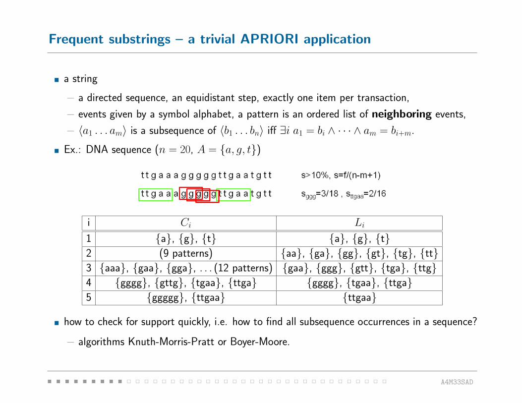
� a string

− a directed sequence, an equidistant step, exactly one item per transaction,

− events given by a symbol alphabet, a pattern is an ordered list of neighboring events,

− 〈a1 . . . am〉 is a subsequence of 〈b1 . . . bn〉 iff ∃i a1 = bi ∧ · · · ∧ am = bi+m.

� Ex.: DNA sequence (n = 20, A = {a, g, t})

i Ci Li

1 {a}, {g}, {t} {a}, {g}, {t}2 (9 patterns) {aa}, {ga}, {gg}, {gt}, {tg}, {tt}3 {aaa}, {gaa}, {gga}, . . . (12 patterns) {gaa}, {ggg}, {gtt}, {tga}, {ttg}4 {gggg}, {gttg}, {tgaa}, {ttga} {gggg}, {tgaa}, {ttga}5 {ggggg}, {ttgaa} {ttgaa}

� how to check for support quickly, i.e. how to find all subsequence occurrences in a sequence?

− algorithms Knuth-Morris-Pratt or Boyer-Moore.

� � � � � � � � � � � � � � � � � � � � � � � � � � � � � � � � � � � � � � � A4M33SAD

pCanonical form for sequences

� a canonical (standard) code word

− a unique sequence representation, based on the symbol alphabet ordering,

− a usual (not necessary) choice:

∗ the lexicographical symbol alphabet ordering a < b < c < . . .,

∗ the lexicographically smallest (smaller) code word taken as canonical (bac < cab),

� a directed sequence

− the only interpretation (way of reading), each (sub)sequence is a canonical code word,

� an undirected sequence

− two possible ways of reading = two alternative code words,

− the routine application of lexicographical ordering is not possible,

− prefix property in a space of canonical code words does not hold:

∗ every prefix of a canonical word is a canonical word itself,

sequence canonical form prefix canonical form

bab bab ba ab

cabd cabd cab bac

− we have to find a different way of forming code words.

� � � � � � � � � � � � � � � � � � � � � � � � � � � � � � � � � � � � � � � A4M33SAD

pCanonical form for undirected sequences

� The canonical code words with the prefix property will be formed as follows

− even and odd length words will be handled separately,

− code words are started in the middle of sequence,

even length odd length

sequence am am−1 . . . a2 a1 b1 b2 . . . bm−1 bm am am−1 . . . a2 a1 a0 b1 b2 . . . bm−1 bmcode word a1 b1 a2 b2 . . . am−1 bm−1 am bm a0 a1 b1 a2 b2 . . . am−1 bm−1 am bmcode word b1 a1 b2 a2 . . . bm−1 am−1 bm am a0 b1 a1 b2 a2 . . . bm−1 am−1 bm am

� canonical is the lexicographically smaller code word in the table,

� the sequence is extended by adding

− a pair am+1 bm+1 or bm+1 am+1,

− one item at the front and one item at the end.

� an example

even length odd length

sequence code words sequence code words

at at ta ule lue leu

data atda taad rules luers leusr

� � � � � � � � � � � � � � � � � � � � � � � � � � � � � � � � � � � � � � � A4M33SAD

pCanonical form for undirected sequences – efficiency

� two possible code words can be created and compared in O(m),

� an additional symmetry flag introduced for each sequence enables the same in O(1)

sm =

m∧i=1

(ai = bi)

� the symmetry flag is maintained in constant time with

sm+1 = sm ∧ (am+1 = bm+1)

� sequence extension is permissible when the flag:

− if sm = true, it must be am+1 ≤ bm+1,

− if sm = false, any relation between am+1 and bm+1 is possible.

� sequences and symmetry flags at the beginning

− even length: an empty sequence, s0 = 1,

− odd length: all frequent alphabet symbols, s1 = 1,

� the procedure guarantees exclusively the canonical sequence extensions.

� � � � � � � � � � � � � � � � � � � � � � � � � � � � � � � � � � � � � � � A4M33SAD

pFrequent subsequences – APRIORI application to undirected sequences

� consider undirected sequences, otherwise the formalization as yet

− 〈a1 . . . am〉 is a subsequence of 〈b1 . . . bn〉 if:

∃i a1 = bi ∧ · · · ∧ am = bi+m, or

∃i a1 = bi+m ∧ · · · ∧ am = bi,

� ex.: DNA sequence (n = 20, A = {a, g, t})

i Ci Li

0 {} {}1 {a}, {g}, {t} {a}, {g}, {t}2 {aa}, {ag}, {at}, {gg}, {gt}, {tt} {aa}, {gg}, {gt}, {tt}3 {aaa}, {aag}, {aat}, {gag}, {gat}, {tat}, {aga}, {agg}, {agt}, {ggg}, {gtt}{ggg}, {ggt}, {tgt}, {ata}, {atg}, {att}, {gtg}, {gtt}, {ttt}

4 {aaaa}, {aaag}, {aaat}, {gaag}, {gaat}, {taat}, {gggg}{agta}, {agtg}, {ggta}, {agtt}, {tgta}, {ggtg},{ggtt}, {tgtg}, . . . in total 27 (1) patterns

� � � � � � � � � � � � � � � � � � � � � � � � � � � � � � � � � � � � � � � A4M33SAD

pA generalized subsequence definition in transactional representation

� Items: I = {i1, i2, . . . , im},� itemsets: (x1, x2, . . . , xk) ⊆ I , k ≥ 1, xi ∈ I ,

� sequences: 〈s1, . . . , sn〉, si = (x1, x2, . . . , xk) ⊆ I , si 6= ∅, x1 < x2 < . . . < xk,

− an ordered list of elements, elements = itemsets,

− the canonical representation: lexicographical ordering of items in each itemset,

− ex.: 〈a(abc)(ac)d(cf )〉, a simplification of the form: (xi) ∼ xi,

� the sequence length l (l-sequence)

− given by the number of item instances (occurrences) in sequence,

− ex.: 〈a(abc)(ac)d(cf )〉 is a 9-sequence,

� α is a subsequence of β, β is a supersequence of α: α v β

− α = 〈a1, . . . , an〉, β = 〈b1, . . . , bm〉, ∃1 ≤ j1 < . . . < jn ≤ m,∀i = 1 . . . n : ai ⊆ bji,

− ex.: 〈a(bc)df〉 v 〈a(abc)(ac)d(cf )〉, 〈d(ab)〉 6v 〈a(abc)(ac)d(cf )〉,− non-contiguous sequential patterns,

� a sequence database: S = {〈sid1, s1〉 . . . , 〈sidk, sk〉}

− a set of ordered pairs a sequence identifier and a sequence.

� � � � � � � � � � � � � � � � � � � � � � � � � � � � � � � � � � � � � � � A4M33SAD

pSubsequence search in transaction representation

� Support of α sequence in the database S

− the number of sequences s ∈ S satisfying: α v s,

� Subsequence search in transaction representation, task definition

− input: S a smin – minimum support,

− output: the complete set of frequent sequential patterns

∗ all the subsequences with or above the threshold frequency.

Id Sequence

10 〈a(abc)(ac)d(cf )〉20 〈(ad)c(bc)(ae)〉30 〈(ef )(ab)(df )cb〉40 〈eg(af )cbc〉

Id Time Items

10 t1 a

10 t2 a, b, c

10 t3 a, c

10 t4 d

10 t5 c, f

l sequential pattern (smin=2)

3 〈a(bc)〉, 〈aba〉, 〈abc〉, 〈(ab)c〉, 〈(ab)d〉, 〈(ab)f〉, 〈aca〉, 〈acb〉, 〈acc〉, 〈adc〉, . . .4 〈a(bc)a〉, 〈(ab)dc〉, . . .

Pei, Han et al.: PrefixSpan: Mining Sequential Patterns by Prefix-Projected Growth.

� � � � � � � � � � � � � � � � � � � � � � � � � � � � � � � � � � � � � � � A4M33SAD

pGSP: Generalized Sequential Patterns [Agrawal, Srikant, 1996]

� applies the core idea of APRIORI to sequential data,

� the key issue is generation of the candidate sequential patterns

− divided into two steps

1. join

∗ l-sequence is created by joining of two (l-1)-sequences,

∗ (l-1)-sequences can be joined when identical after removal of the first item in one

and the last one in second,

2. prune

∗ skip each l-sequence which contains an infrequent (l-1)-subsequence.

L3C4

after join after prune

〈(ab)c〉, 〈(ab)d〉, 〈(ab)(cd)〉 〈(ab)(cd)〉〈a(cd)〉, 〈(ac)e〉, 〈(ab)ce〉〈b(cd)〉, 〈bce〉

Agrawal, Srikant: Mining Sequential Patterns: Generalizations and Performance.

� � � � � � � � � � � � � � � � � � � � � � � � � � � � � � � � � � � � � � � A4M33SAD

pExample: GSP, smin=2

Id Sequence

10 〈(bd)cb(ac)〉20 〈(bf )(ce)b(fg)〉30 〈(ah)(bf )abf〉40 〈(be)(ce)d〉50 〈a(bd)bcb(ade)〉

� s(〈g〉) = s(〈h〉) = 1 < smin

(skips a large portion of 92 available 2-candidates),

� 〈(bd)cba〉 v s10 ∧ 〈(bd)cba〉 v s50

(created from 〈(bd)cb〉 a 〈dcba〉),

(the patterns 〈(bd)ba〉, 〈(bd)ca〉 and 〈bcba〉 must also

be frequent).

� � � � � � � � � � � � � � � � � � � � � � � � � � � � � � � � � � � � � � � A4M33SAD

pAPRIORI algorithm for sequences – disadvantages

� the generate (join step) and test (prune step) method,

� the problems discussed in terms of frequent itemsets persist and intensify

1. generates a large amount of candidate patterns

− obvious even for 2-sequences: m×m + m(m−1)2 → O(m2)

(for itemsets it was just the second fraction, one third or so of candidates),

2. requires a lot of database scans

− one scan per sequence length,

− the number of scans given by the max pattern length

the length ≤ max(|s|, s ∈ S) (typically >> m),

(max itemset length is m and thus m scans at most),

3. search for long sequential patterns is difficult

− the total amount of candidate patterns is exponential with the pattern length,

(the same growth as for itemsets, however the problem max(|s|, s ∈ S) >> m).

� the disadvantages addressed by alternative methods

− FreeSpan and PrefixSpan algorithms as examples.

� � � � � � � � � � � � � � � � � � � � � � � � � � � � � � � � � � � � � � � A4M33SAD

pEpisode rules

� association rule analogy for sequences,

� predict the further development of sequence with the aid of patterns,

� S is a sequence database, β a frequent subsequence and α is its prefix,

� episode rule is a probabilistic implication

− α⇒ postfix(β, α),

− if conf (α⇒ postfix(β, α)) = s(β,S)s(α,S) ≥ confmin.

Id Sequence

10 〈(bd)cb(ac)〉20 〈(bf )(ce)b(fg)〉30 〈(ah)(bf )abf〉40 〈(be)(ce)d〉50 〈a(bd)bcb(ade)〉

� let smin = 2, confmin = 0.7

� β = 〈(bd)cba〉, α = 〈(bd)〉

conf (〈(bd)〉 ⇒ 〈cba〉) = 1 ≥ confmin,

� β = 〈bcb〉, α = 〈bc〉

conf (〈bc〉 ⇒ 〈b〉) = 34 ≥ confmin,

� when dealing with a single sequence S the support definition works with constraints

− (adjoining) sequence elements must not be too far (MaxGap),

− only the minimal occurences of a sequence are considered.

� � � � � � � � � � � � � � � � � � � � � � � � � � � � � � � � � � � � � � � A4M33SAD

pFrequent subgraph mining: definition

� given: graphs G = {G1, . . . , Gn} with labels A = {a1, . . . , am} and minimum support smin

� output: the set of frequent (sub)graphs with support meeting the minimum threshold

− FG(smin) = {S | sG(S) ≥ smin},

� common constraint

− connected subgraphs only,

� main problem

− to avoid redundancy when searching

∗ canonical representation of (sub)graphs,

∗ partial order of (sub)graph space,

∗ efficient pruning of the searched subgraph space,

∗ fragment repository for processed graphs.

� subgraph S ⊆ G

− informally: omit some vertices and (their incident) edges,

− proper subgraph S ⊂ G, cannot be identical with the original graph,

− NP-complete subgraph isomorphism problem needs to be solved to count support!

� � � � � � � � � � � � � � � � � � � � � � � � � � � � � � � � � � � � � � � A4M33SAD

pFrequent subgraphs: example

� G contains three molecules, minimum support smin = 2,

� 15 frequent subgraphs exist,

� empty graph is properly contained in all graphs by definition.

Borgelt: Frequent Pattern Mining. The same for the rest of the presentation.

� � � � � � � � � � � � � � � � � � � � � � � � � � � � � � � � � � � � � � � A4M33SAD

pTypes of frequent subgraphs – closed and maximal

� maximal subgraph

− is frequent but none of its proper supergraphs is frequent,

− the set of maximal (sub)graphs:

MG(smin) = {S | sG(S) ≥ smin ∧ ∀R ⊃ S : sG(R) < smin},− every frequent (sub)graph has a maximal supergraph,

− no supergraph of a maximal (sub)graph is frequent,

− MG(smin) does not preserve knowledge of support values of all frequent subgraphs,

� closed subgraph

− is frequent but none of its proper supergraphs has the same support,

− the set of closed (sub)graphs:

CG(smin) = {S | sG(S) ≥ smin ∧ ∀R ⊃ S : sG(R) < sG(S)},− every frequent (sub)graph has a closed supergraph (with the identical support),

− CG(smin) preserves knowledge of support values of all frequent subgraphs,

− every maximal subgraph is also closed.

� � � � � � � � � � � � � � � � � � � � � � � � � � � � � � � � � � � � � � � A4M33SAD

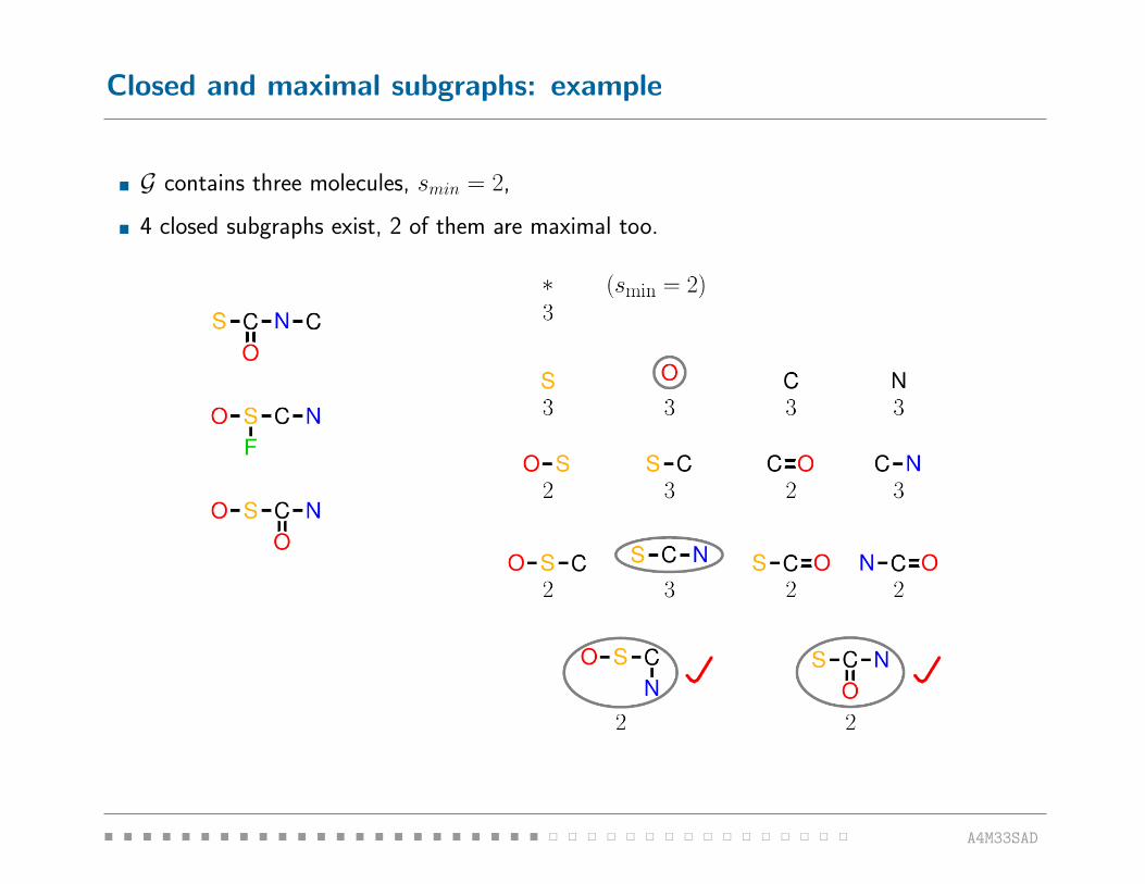
pClosed and maximal subgraphs: example

� G contains three molecules, smin = 2,

� 4 closed subgraphs exist, 2 of them are maximal too.

� � � � � � � � � � � � � � � � � � � � � � � � � � � � � � � � � � � � � � � A4M33SAD

pPartially ordered set of subgraphs and its search

� subgraph (isomorphism) relationship defines a partial order on subgraphs

− Hasse diagram exists, the empty graph makes its infimum, no natural supremum exists,

− diagram can be completely searched top-down from the empty graph,

− branching factor is large, the depth-first search is usually preferable.

� the main problem

− a (sub)graph can be grown in several different ways,

− diagram must be turned into a tree – each subgraph has a unique parent.

� � � � � � � � � � � � � � � � � � � � � � � � � � � � � � � � � � � � � � � A4M33SAD

pPartially ordered set of subgraphs and its search

� Searching for frequent (sub)graphs in the subgraph tree,

� base loop

− traverse all possible vertex attributes (their unique parent is the empty graph),

− recursively process all vertex attributes that are frequent,

� Recursive processing for a given frequent (sub)graph S

− generate all extensions R of S by an edge or by an edge and a vertex

∗ edge addition (u, v) 6∈ ES, u ∈ VS ∨ v ∈ VS,

∗ if u 6∈ VS ∨ v 6∈ VS, the missing node is added too,

− S must be the unique parent of R,

− if R is frequent, further extend it, otherwise STOP.

� � � � � � � � � � � � � � � � � � � � � � � � � � � � � � � � � � � � � � � A4M33SAD

pAssigning unique parents

� How can we formally define the set of parents of subgraph S?

− subgraphs that contain exactly one edge less than the subgraph S,

− in other words, all the maximal proper subgraphs,

� canonical (unique) parent pc(S) of subgraph S

− an order on the edges of the (sub)graph S must be given before,

− let e∗ be the last edge in the order whose removal does not diconnect S

∗ then pc(S) is the graph S without the edge e∗,

∗ if e∗ leads to a leaf, we can remove it along with the created isolated node,

− if e∗ is the only edge of S, we also need an order of the nodes,

� in order to define an order of the edges we will rely on a canonical form of (sub)graphs

− each (sub)graph is described by a code word,

− it unambiguously identifies the (sub)graph (up to automorphism = symmetries),

− having multiple code words per graph

∗ one of them is (lexicographically) singled out as the canonical code word.

� � � � � � � � � � � � � � � � � � � � � � � � � � � � � � � � � � � � � � � A4M33SAD

pCanonical graph representation

� Basic idea

− the characters of the code word describe the edges of the graph,

− vertex labels need not be unique, they must be endowed with unique labels (numbers),

� usual requirement on canonical form

− prefix property, which means that . . .

− when the last edge e∗ is removed, the canonical word of the canonical parent originates,

� assuming the prefix property holds, search algorithm takes the canonical word of a parent and

− generates all possible extensions by an edge (and maybe a vertex),

− checks whether the extended code words are the canonical code words,

− consequence: easy and non-redundant access to children,

� the most common canonical forms

− spanning tree,

− adjacency matrix.

� � � � � � � � � � � � � � � � � � � � � � � � � � � � � � � � � � � � � � � A4M33SAD

pCanonical forms based on spanning trees

� Graph code word is created when constructing a spanning tree of the graph

− numbering the vertices in the order in which they are visited,

− describing each edge by the numbers of incident vertices, the edge and vertex labels,

− listing the edge descriptions in the order in which the edges are visited

(edges closing cycles may need special treatment),

� the most common ways of constructing a spanning tree are

− search: depth-first × breadth-first,

− both approaches ask for their own way of code word construction,

� one graph may be described by a large number of code words

− a graph has multiple spanning trees and its traversals (initial vertex, branching options),

− the main problem is to find the lexicographically smallest = canonical word quickly.

� � � � � � � � � � � � � � � � � � � � � � � � � � � � � � � � � � � � � � � A4M33SAD

pCanonical forms based on spanning trees

� A precedence order of labels is introduced

− due to efficiency, frequency of labels shall be concerned,

− vertex labels are recommended to be in ascending order,

� Regular expressions for code words

− depth-first: a (id is b a)m,

(exception: indices in decreasing order)

− meaning of symbols:

n the number of vertices of the graph,

m the number of edges of the graph,

is index of the source vertex of an edge, is ∈ {0, . . . , n− 1},id index of the destination vertex of an edge, id ∈ {0, . . . , n− 1},a the attribute of a vertex,

b the attribute of an edge.

� � � � � � � � � � � � � � � � � � � � � � � � � � � � � � � � � � � � � � � A4M33SAD

pCanonical spanning tree: example

� Order of labels

− elements (vertices): S ≺ N ≺ O ≺ C, bonds (edges): − ≺ =,

� A code word

A: S 10-N 21-O 31-C 43-C 54-O 64=O 73-C 87-C 80-C

� � � � � � � � � � � � � � � � � � � � � � � � � � � � � � � � � � � � � � � A4M33SAD

pRecursive checking for canonical form

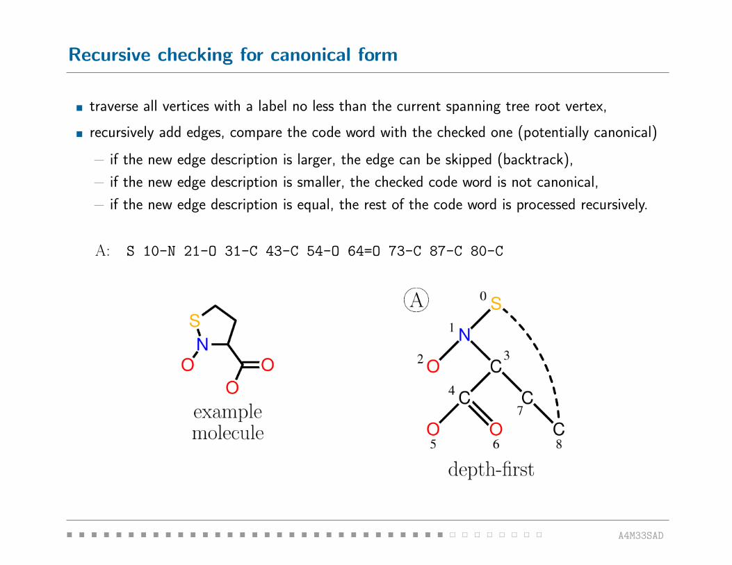
� traverse all vertices with a label no less than the current spanning tree root vertex,

� recursively add edges, compare the code word with the checked one (potentially canonical)

− if the new edge description is larger, the edge can be skipped (backtrack),

− if the new edge description is smaller, the checked code word is not canonical,

− if the new edge description is equal, the rest of the code word is processed recursively.

A: S 10-N 21-O 31-C 43-C 54-O 64=O 73-C 87-C 80-C

� � � � � � � � � � � � � � � � � � � � � � � � � � � � � � � � � � � � � � � A4M33SAD

pRestricted extensions of canonical words

� Principle of recursive search of subgraph tree

− generate all possible extensions of a given canonical code word (of a frequent parent),

− extension = add the description of an edge at the end of the code word,

− canonical form is checked, if met then proceed recursively, otherwise the word is discarded,

� how to verify efficiently whether a word is canonical?

− in general, a lex. smaller word with the same root vertex needs to be found,

− simple local rules exist that reject extensions locally = immediately

∗ only certain vertices are extendable,

∗ certain cycles cannot be closed,

∗ they represent necessary canonicity conditions, not sufficient.

� � � � � � � � � � � � � � � � � � � � � � � � � � � � � � � � � � � � � � � A4M33SAD

pRestricted extensions of canonical words

� Depth-first: rightmost path extension

− extendable vertices

∗ must be on the rightmost path of the spanning tree

(other vertices cannot be extended in the given search-tree branch),

∗ if the source vertex of the new edge is not a leaf, the edge description must not precede

the description of the downward edge on the path

(the edge attribute must be no less than the edge attribute of the downward edge,

if it is equal, the attribute of its destination vertex must be no less than the attribute

of the downward edge’s destination vertex),

− edges closing cycles

∗ must start at an extendable vertex,

∗ must lead to the rightmost leaf

(a subgraph has only one vertex meeting the condition),

∗ the index of the source vertex must precede the index of the source vertex of any edge

already incident to the rightmost leaf.

� � � � � � � � � � � � � � � � � � � � � � � � � � � � � � � � � � � � � � � A4M33SAD

pRestricted extensions: examples

� Extendability

− vertices: 0, 1, 3, 7, 8,

− edges closing cycles: none,

� Extension: attach a single bond carbon atom at the leftmost oxygen atom

A: S 10-N 21-O 31-C 43-C 54-O 64=O 73-C 87-C 80-C 92-C

S 10-N 21-O 32-C · · ·

� � � � � � � � � � � � � � � � � � � � � � � � � � � � � � � � � � � � � � � A4M33SAD

pFrequent subgraphs: use of restricted extensions

� Crossed-arc extension gets immediately rejected,

� bottom-right graph is visited from its upper-right canonical parent (prefix) only,

� see the canonical code words:

upper left: S 10-N 21-O 31-C 43-C 54-O 64=O 73-C 87-C 80-C

bottom left: S 10-N 21-O 31-C 43-C 54-O 64=O 73-C 87-C 80-C 90-O

upper right: S 10-N 21-O 32-C 41-C 54-C 65-O 75=O 84-C 98-C

bottom right: S 10-N 21-O 32-C 41-C 54-C 65-O 75=O 84-C 98-C 90-C

� � � � � � � � � � � � � � � � � � � � � � � � � � � � � � � � � � � � � � � A4M33SAD

pFrequent subgraphs search with canonical form

� Start with a single seed vertex,

� add an edge (and maybe a vertex) in each step (restricted extensions),

� determine the support and prune infrequent (sub)graphs (outside the code word space),

� check for canonical form and prune (sub)graphs with non-canonical code words.

� � � � � � � � � � � � � � � � � � � � � � � � � � � � � � � � � � � � � � � A4M33SAD

pAdditional issues

� Fragment repository

− canonical code words represent the dominant approach to redundancy reduction,

− an alternative is to store already processed subgraphs, they are not processed again,

− key efficiency issues: memory, fast access (hash),

� extensions for molecules

− frequent molecular fragments processed en bloc,

− ring mining, carbon chains and wildcard vertices,

� single graph only

− distinct definition of support (more complex),

� trees

− ordered × unordered, rooted × unrooted,

− in general easier than unrestricted graphs.

� � � � � � � � � � � � � � � � � � � � � � � � � � � � � � � � � � � � � � � A4M33SAD

pFrequent subsequence/subgraph mining – summary

� Problem closely related to frequent itemset mining

− APRIORI property,

� however, to avoid redundancy during search gets more difficult

− larger branching factor,

− unlike complex patterns, itemsets have no internal structure,

� non-trivial canonical sequence/graph representation

− guarantees that support is counted at most once

(additional necessary condition is parental support),

− choice of representation related with choice of searching algorithm,

− prefix property allows for early rejection of non-canonical candidates,

− the canonical form based on spanning trees introduced,

� support checking gets more time consuming

− e.g., subgraph isomorphism test for two graphs is NP-complete,

� special pattern types get dedicated treatment

− e.g., generalized sequences with gap constraints.

� � � � � � � � � � � � � � � � � � � � � � � � � � � � � � � � � � � � � � � A4M33SAD

pRecommended reading, lecture resources

:: Reading

� Agrawal, Srikant: Mining Sequential Patterns.

� Agrawal, Srikant: MSPs: Generalizations and Performance.

− from APRIORI towards its sequential versions AprioriAll and GSP,

− http://citeseerx.ist.psu.edu/viewdoc/download?doi=10.1.1.95.2818&rep=rep1&type=pdf,

� Mannila et al.: Discovery of Frequent Episodes in Event Sequences.

− episodal rules,

− http://citeseerx.ist.psu.edu/viewdoc/summary?doi=10.1.1.49.3594,

� Borgelt: Frequent Pattern Mining.

− both frequent subsequence and subgraph mining, detailed slides,

− http://www.borgelt.net/teach/fpm/slides.html.

� � � � � � � � � � � � � � � � � � � � � � � � � � � � � � � � � � � � � � � A4M33SAD