mining traffic incidents to forecast impacturbcomp2012/papers/urbcomp2012_paper32... · mining...
TRANSCRIPT
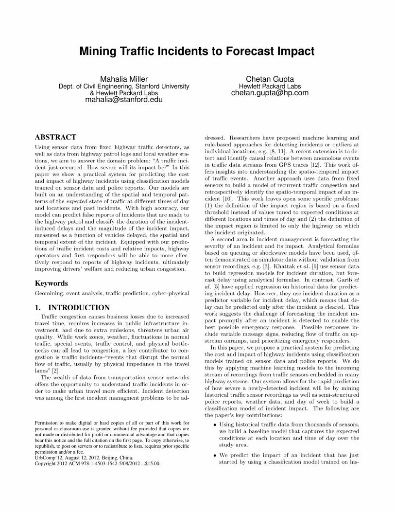
Mining Traffic Incidents to Forecast Impact
Mahalia MillerDept. of Civil Engineering, Stanford University
& Hewlett Packard [email protected]
Chetan GuptaHewlett Packard Labs
ABSTRACTUsing sensor data from fixed highway traffic detectors, aswell as data from highway patrol logs and local weather sta-tions, we aim to answer the domain problem: “A traffic inci-dent just occurred. How severe will its impact be?” In thispaper we show a practical system for predicting the costand impact of highway incidents using classification modelstrained on sensor data and police reports. Our models arebuilt on an understanding of the spatial and temporal pat-terns of the expected state of traffic at different times of dayand locations and past incidents. With high accuracy, ourmodel can predict false reports of incidents that are made tothe highway patrol and classify the duration of the incident-induced delays and the magnitude of the incident impact,measured as a function of vehicles delayed, the spatial andtemporal extent of the incident. Equipped with our predic-tions of traffic incident costs and relative impacts, highwayoperators and first responders will be able to more effec-tively respond to reports of highway incidents, ultimatelyimproving drivers’ welfare and reducing urban congestion.
KeywordsGeomining, event analysis, traffic prediction, cyber-physical
1. INTRODUCTIONTraffic congestion causes business losses due to increased
travel time, requires increases in public infrastructure in-vestment, and due to extra emissions, threatens urban airquality. While work zones, weather, fluctuations in normaltraffic, special events, traffic control, and physical bottle-necks can all lead to congestion, a key contributor to con-gestion is traffic incidents–“events that disrupt the normalflow of traffic, usually by physical impedance in the travellanes” [2].
The wealth of data from transportation sensor networksoffers the opportunity to understand traffic incidents in or-der to make urban travel more efficient. Incident detectionwas among the first incident managment problems to be ad-
Permission to make digital or hard copies of all or part of this work forpersonal or classroom use is granted without fee provided that copies arenot made or distributed for profit or commercial advantage and that copiesbear this notice and the full citation on the first page. To copy otherwise, torepublish, to post on servers or to redistribute to lists, requires prior specificpermission and/or a fee.UrbComp’12, August 12, 2012. Beijing, China.Copyright 2012 ACM 978-1-4503-1542-5/08/2012 ...$15.00.
dressed. Researchers have proposed machine learning andrule-based approaches for detecting incidents or outliers atindividual locations, e.g. [8, 11]. A recent extension is to de-tect and identify causal relations between anomolous eventsin traffic data streams from GPS traces [12]. This work of-fers insights into understanding the spatio-temporal impactof traffic events. Another approach uses data from fixedsensors to build a model of recurrent traffic congestion andretrospectively identify the spatio-temporal impact of an in-cident [10]. This work leaves open some specific problems:(1) the definition of the impact region is based on a fixedthreshold instead of values tuned to expected conditions atdifferent locations and times of day and (2) the definition ofthe impact region is limited to only the highway on whichthe incident originated.
A second area in incident management is forecasting theseverity of an incident and its impact. Analytical formulaebased on queuing or shockwave models have been used, of-ten demonstrated on simulator data without validation fromsensor recordings, e.g. [3]. Khattak et al. [9] use sensor datato build regression models for incident duration, but fore-cast delay using analytical formulae. In contrast, Garib etal. [5] have applied regression on historical data for predict-ing incident delay. However, they use incident duration as apredictor variable for incident delay, which means that de-lay can be predicted only after the incident is cleared. Thiswork suggests the challenge of forecasting the incident im-pact promptly after an incident is detected to enable thebest possible emergency response. Possible responses in-clude variable message signs, reducing flow of traffic on up-stream onramps, and prioritizing emergency responders.
In this paper, we propose a practical system for predictingthe cost and impact of highway incidents using classificationmodels trained on sensor data and police reports. We dothis by applying machine learning models to the incomingstream of recordings from traffic sensors embedded in manyhighway systems. Our system allows for the rapid predictionof how severe a newly-detected incident will be by mininghistorical traffic sensor recordings as well as semi-structuredpolice reports, weather data, and day of week to build aclassification model of incident impact. The following arethe paper’s key contributions:
• Using historical traffic data from thousands of sensors,we build a baseline model that captures the expectedconditions at each location and time of day over thestudy area.
• We predict the impact of an incident that has juststarted by using a classification model trained on his-

torical events. We show that combining traffic sensorrecordings, initial police reports, weather data, andtime of day we are able to reliably predict absoluteand relative impact of a highway incident. We mea-sure the impact by the duration of incident-induceddelays and by economic losses from cumulative traveltime delay 1.
• We demonstrate the high predictive power of our modelon two real datasets of reported highway incidents fromdifferent regions, each over a two-month period. Wealso show the high level of transfer learning possibleby training our model on one region and testing themodel on incidents from a different year and region.
Although in this work our framework is specifically ap-plied to traffic, our approach points a way toward studyingthe impact of events in other operational domains in whichwe have sensor data and external incident (event) logs 2.
2. INCIDENT IMPACT COMPUTATIONWe first introduce relevant definitions and then outline
an algorithm to identify the impact region for a particularincident considering the true road topology.
2.1 PreliminariesIn this work, we analyze contiguous sections of freeway.
We use data from the California Performance MeasurementSystem 3) where tens of thousands of loop detectors fixedalong major highways statewide measure quantities such asvelocity, density, and flow every 30 seconds. For incidents,we use data from the California Highway Patrol (CHP)4.When an incident is reported, CHP notes details such aswhen and where it occurred. We provide further details inSection 4.1.
We model the regional highway network as a spatial net-work graph, G = (U,E). Each node represents a detector, ui
(located at postmile xi) and an edge ei,j exists for every pairof detectors such that there is a single road segment betweentwo sensors where the road segment is part of a highway withPeMS detectors. The edge ei,j is directed such that j is up-stream of i, where upstream is defined as in the oppositedirection of normal traffic flow. In practice, at detector ui,the vehicle count data is aggregated over all lanes to com-pute the total recorded flow in a given direction during afive-minute time window. This quantity known as flow isdenoted by q(i, t) with units in vehicles per hour (vph). Theaverage occupancy of the highway over all lanes in the givendirection is denoted by ρ(i, t), with 0 ≤ ρ(i, t) ≤ 1, where 0indicates an empty highway and 1 indicates the theoretical
1The economic losses in this context are the sum over theestimated number of affected vehicles of the extra time overexpected travel times spent in the impact region of the inci-dent multiplied by a cost per hour of lost productivity fromthe US Department of Transportation [1]2This work is part of a larger effort called Live OperationalIntelligence (LOI)[6], in which we are building systems forclients that analyze large amounts of streaming sensor andevent data for supporting operational decisions. Interestedindustries include oil and gas production and drilling, energydelivery, logistics and transportation.3Freeway Performance Measurement System (PeMS),http://pems.dot.ca.gov4Also avaiable at http://pems.dot.ca.gov
limit of full coverage of the road by vehicles [4]. The flow-weighted mean velocity v(i, t) at location i and time t is thechosen measure for the vehicle speed at a given location iand time t:
v(i, t) =
∑Nlk=1 qk(i, t)vk(i, t)∑Nl
k=1 qk(i, t)(1)
where the speed vk(i, t) for each lane k and at detector i andat time t is computed according to the algorithm describedby Chen [4].
Critical for determining abnormal traffic behavior is theidentification of recurrent traffic conditions. Kwon [10] usea nearest-neighbor approach to find k days that had trafficconditions similar to the traffic conditions just before thestart of an incident of interest. The average of the condi-tions at k-days is then taken to be the recurrent (or normal)behavior. For small k, the method leads to the possibility ofchoosing a date in the past with an incident—the oppositeof trying to find recurrent non-incident conditions. Insteadof using nearest-neighbors, we calculate the median of thespeeds at each sensor location i and each point in time t andcall it the recurrent velocity, v∗(i, t). The median is robustto outliers, i.e. to incidents.
2.2 Understanding Cost of DelayIn this work, the economic loss due to lost productivity
associated with an incident is directly proportional to thecumulative incident delay value according to the cost-benefitframework used in the State of California [1]. Thus, we willnow detail the computation of the cumulative delay for alldrivers in an incident impact region.
The delay on each road segment per unit of time is de-fined as the additional vehicle-hours traveled driving belowfree-flow speed, vref , per unit of time. In this study vref is60 mph as is standard with other researchers using similardata [10]. This analysis further assumes that the flow, occu-pancy, and speed remain constant during every five-minuteinterval per road segment. We begin with the standard do-main definition of delay d(i, t) in the road segment of lengthli starting at detector i at time t. The delay essentially mea-sures the vehicle-hours lost due to traveling below referencevelocity [13]:
d(i, t) = li × q(i, t)×max
(1
v(i, t)− 1
vref, 0
)(2)
where v(i, t) refers to velocity at location i and time t asdiscussed in 2.1, q(i, t) is the flow at location i and timet and vref is considered to be constant for all time t andlocation i with a value equal to 60 mph.
We are interested in the cumulative delay for all affecteddrivers, not simply the per segment per unit time delay,d(i, t). Thus integrating d(i, t) over a region A and time in-terval T the total delay over the spatial and temporal regiondefined by A and T would be given as
Dtot =
∫A
∫T
d(i, t)dudt. (3)
The total delay over region A and time T can have manycauses. An approach as described by Kwon and Varaiya [10]is to separate total delay as follows:
Dtot = Dinc +Drec +Drem (4)

where Dtot is total delay calculated from flow and speed,Dinc is the delay caused by non-recurring incidents such ascollisions (Dinc is referred to as Dcol in [10]), Drec is therecurrent delay and Drem is the remaining delay. Of ourinterest is Dinc, which is computed over a contiguous regioncalled the impact region of an incident. The work of previousresearchers to divide delay into components offers a generalframework, but there is no work to date that mathematicallyderives expressions that capture the different terms. We nowprovide a derivation of the various components of delay.
We begin by defining an impact region, which we under-stand to be a contiguous region (contiguous in both spaceand time) beginning at the time and location of the incident,and where the traffic conditions deviate from the recurrenttraffic patterns. This contiguous region goes forward in timeand upstream in space, since after an incident, traffic backsup (Figure 1 illustrates the spread of the impact region withtime for an example incident). Precisely, let the closest up-stream sensor to incident Ia denoted by ua and the time ofincident Ia be ta. Then:
Definition 1. The impact region is collection of connectedsubgraphs At induced from G. At is constructed for eachtime t starting at t = ta, such that for all nodes i ∈ At, ei-ther v(i, t−1) < v∗(i, t−1) or v(P (i), t−1) < v∗(P (i), t−1)where P (i) is the parent of the detector i. At ta, Ata is ua.
Now we can derive some related quantities. SubstitutingEquation 2 into Equation 3 and replacing the integral withsummation (since measurements are discrete), Equation 3can be rewritten as
Dtot =∑
T
∑A li × q(i, t)
×max(
1v(i,t)
− 1v∗(i,t) + 1
v∗(i,t) −1
vref, 0).
(5)
Equation 5 shows that the delay is trivially 0 when the cur-rent speed is greater than the free-flow speed, i.e., v(i, t) ≥vref . Equation 5 allows a rewriting of the total delay intotwo non-zero delay cases, as defined below:
1. Current speed is below the threshold speed and thefree-flow speed, v(i, t) < v∗(i, t) ≤ vref .
Dtot =∑
T
∑A li × q(i, t)×
(1
v(i,t)− 1
v∗(i,t)
)+∑
T
∑A li × q(i, t)×
(1
v∗(i,t) −1
vref
)(6)
2. Current speed is greater than the threshold speed butless than the free-flow speed, v∗(i, t) ≤ v(i, t) ≤ vref .
Dtot =∑
T
∑A li × q(i, t)×max
(1
v(i,t)− 1
vref, 0)
(7)
For the sake of simplicity, it is assumed that each spatio-temporal region of delay is caused by a unique delay-causingincident. So, when computing the impact region of an inci-dent, we do not include regions corresponding to the startof a subsequent incident. Now, let At be the spatial extentof a particular incident’s impact at time t ∈ T ′ where T ′ isits temporal extent. Then,∑
T
∑Atli × q(i, t)×
(1
v(i,t)− 1
v∗(i,t)
)=∑′
T
∑Atli × q(i, t)×
(1
v(i,t)− 1
v∗(i,t)
)+
∑T−T ′
∑A−At
li × q(i, t)×(
1v(i,t)
− 1v∗(i,t)
).
(8)
Combining Equation 4, which states that Dtot = Dinc +Drec +Drem, with Equations 6, 7 and 8 yields the followingdefinitions for Dinc, Drem and Dtot:
Definition 2.
If v(i, t) < v∗(i, t),
Dinc =∑
T ′∑
Atli × q(i, t)×
(1
v(i,t)− 1
v∗(i,t) ))
Drem =∑
T−T ′∑
A−Atli × qi(t)×
(1
vi(t)− 1
v∗(i,t)
)Drec =
∑T
∑A li × q(i, t)×
(1
v∗(i,t) −1
vref (t)
)If v(i, t) ≥ v∗(i, t),Dinc = Drem = 0Drec =
∑T
∑A li × q(i, t)
×max(
1v(i,t)
− 1vref (t)
, 0).
(9)
These equations precisely define quantities that can be un-derstood as calculating the cumulative extra travel time ex-perienced by all drivers during a certain time period andspatial region when traffic is not freely flowing (v < vref ).The recurrent delay, Drec, is the component of the currentlyexperienced delay that drivers might always expect travelingthrough a region during a certain time of day. The incidentdelay, Dinc, is the cumulative extra time that all driversspend in traffic associated with a given incident. The equa-tions essentially codify our intuition that: if the current ve-locity v(i, t) is below the expected velocity v∗(i, t), then onecomponent is the recurrent delay (from vref to v∗(i, t)) andthe remaining component (from v∗(i, t) to v(i, t)) is eitherincident delay if we are in an incident region or remainingdelay otherwise. If the current velocity is above the expectedvelocity, all of the delay is the recurrent delay. The cost ofan incident is then simply a constant dollar amount timesDinc (We take it to be $11.20 for California [1].)
2.3 Computing Duration and Cost of DelayNow that we have defined the impact region and cost of
delay, we will briefly outline our algorithm for computingthe delay associated with an incident.
We define the set of detectors of congested segments attime t = 0 as a group of detectors in which the speed ateach detector is below the variable threshold speed, v∗(i, 0),as defined in 2.1. Note that in published algorithms to date,e.g. [10], a fixed threshold speed such as 50mph has beenused to determine membership in the preliminary impactregion.
Intuitively, for each incident, a ∈ A, we begin at ta withthe closest upstream sensor ua. Our algorithm continuesin the next time steps t > 0 and a node is appended tothe set, St, of nodes at time t, if the node is congested,i.e., if the flow-averaged speed is less than (1 − c)v∗(i, t),(where c is a constant), and the sensor was congested in theprevious time step or is directly upstream of a congestedsensor at time t. If the speed is greater than (1 − c)v∗(i, t)and less than (1+c)v∗(i, t) and if the speed at the immediatedownstream sensor was not between (1− c)v∗(i, t) and (1 +c)v∗(i, t), the sensor is appended to the set of congestedsensors at this time step. When both stop conditions, notcongested and no upstream sensors at the previous time step,are met, time is incremented and the search upstream fromua is repeated. The total process of identifying the impactregion for a given incident a ends when St = ∅ at the end of

(a) t = 4 min (b) t = 14 min (c) t = 29 min
Figure 1: Spread of an impact region over time(measured since reported start of the incident)where the congested segments (v(i, t) < v∗(i, t)) areindicated by a bold black line.
a timestep iteration. This allows us to compute the impactregion, At at any time t (In our experiments, we found c =0.05 to be the most suitable). We skip the details for lackof space.
In contrast to the work to date on impact regions [10] inwhich the algorithm identifies congestion on one highway inisolation, our algorithm recursively searches upstream, thusidentifying possible incident impacts to connecting highways.Our algorithm considers the true freeway topology. For ex-ample, Figure 1 shows an example from our Los Angelesdataset that illustrates the automatic incident impact re-gion detection applied to real data. The incident starts inthe southbound direction of the highway at the lower rightof the black line shown in the figures. The incident thenspreads upstream and the impact region spills over onto aconnecting highway temporarily. This figure also illustrateshow our algorithm considers the true road topology.
We are also interested in predicting how long the incidentimpact lasts. We define the duration, ttot, as the durationof the contiguous incident impact region characterized by A′
and T ′. In contrast, the PeMS traffic database system usedin California (URL mentioned before) computes the “dura-tion” of an incident by subtracting the last time stamp ofa police report from the first report. Because this methoddoes not account for effects of an incident after police log re-ports, we instead computed the “duration” directly from thesensor recordings. We compared the durations we computeddirectly from the impact region with those of the police inci-dent logs and found that impact regions tend to last longerthan the PeMS “duration”. In the data, we see examplessuch as one incident with one report of a crash and a secondand final report of an officer dispatched. In this example,our algorithm will compute a longer duration because wemeasure until traffic conditions return to recurrent condi-tions.
3. PREDICTING INCIDENT IMPACT
3.1 Problem DefinitionThe impact of an incident can be characterized in multiple
ways. One possibility might be how much the slowdown willbe at a particular location or another might be predicting ametric over the entire impact region, as previously defined.As mentioned early, we predict the latter—the macro levelimpact caused by an individual incident. The problem is:“Given an incident just occurred, what will its impact be?”We define impact in two ways: (i) The monetary productiv-ity costs of the cumulative non-recurrent delay in Equation9 that will be caused by a particular incident (ii) The du-
ration which can understood to be the temporal extent ofthe impact region. Both metrics are moderately correlatedand are different measures of impact. The cost of delay is aconstant factor accounting for the value of lost time timesthe integration of the delay magnitude over space and time,which could cause incidents of different duration, but dif-ferennt magnitudes, to have the same delay value.
Ideally, we would aim to predict the precise numericalvalues for the two quantities of interest. We tried severalregression techniques and models such as regression trees.We found that predicting the precise values (for either costor duration) is a difficult problem. For example, the leastroot relative square error obtained with regression trees forduration was close to 100% in many cases, meaning thatour error would be the same as if were to make the trivialprediction of the overall mean as the predicted value. Toovercome this, we mapped the problem to predicting theimpact as a class variable. This makes the problem moretractable and from the domain expert level no less useful.Traffic operators are very often satisfied with knowing thegeneral range of the impact, namely “Will the impact benegligible, moderate, or severe?” Or, “Given two incidents,which one will have a greater impact?” Answering thesequestions is the first step to solving the domain-specific needof identifying how to prioritize limited resources to mitigatethe effects of incidents reported to emergency dispatchers.
3.2 Building the Feature VectorA big challenge in predicting impact is building a fea-
ture vector that combines data from disparate structuredand unstructured data sources. The first step is to collectsensor recordings near the incident location. We map a re-ported incident to the closest upstream sensor on the di-rected graph G(U,E). Note that the impact of an incidenttypically spreads upstream, i.e. there is back-up behind anincident (as depicted in Figure 1). At this closest upstreamsensor as well as one directly upstream and one farther up-stream, we collect the current conditions including speedv(i, t), expected speed v∗(i, t), and road occupancy ρ(i, t).Figure 2 depicts the spatial relationship.
Traffic flow
Reported incident location
Closest upstream sensor, “b”
Downstream sensor, “a”
Upstream sensor, “c”
Figure 2: Diagram of sensor locations upstream(“b”, “c’) and downstream (“a”) of the incident.c©Mahalia Miller
In addition to the directly-measured quantities, we com-pute a few meaningful physical quantities such as vdiff (i, t) =v∗(i, t) − v(i, t) at the three sensors in Figure 2. We alsoconstruct a few functions as part of the feature vectors.We aim to capture the physical relationships that definethe traffic through these functions. For example, one func-tion that we compute inspired from Equation 2 is: f(i, t) =q(i, t)× ( 1
v(i,t)− 1
vref).
We then include the second type of data–California High-

way Patrol (CHP) reports since initial testing indicated animprovement in accuracy by including these extra features.In addition to basic information including reported starttime of day, the structured part of the CHP records of-fers a type class (a total of 36 types), which we mapped to9 types: Traffic hazard, Collision+no/minor injuries, Col-lision+major injuries/ambulance, Natural weather hazard,Lane closure, Fire, Collision-no details, Hit and run, Other.We also include features parsed from unstructured policelogs in the first 2 minutes after the reported start of an in-cident.
Another feature we used is whether within one hour of anincident it was raining and if so, by how much.
In addition we considered features pertaining to the topol-ogy of the highways. As of now, we consider the number oflanes as a feature. In future work, we aim to add morefeatures such as the proximity to an exit.
In addition to building feature vectors based on data foreach incident, we construct feature vectors for possible pair-wise combinations of incidents. This dataset is used for pre-dicting which incident of a pair will have relatively higherimpact.
3.3 Bin SelectionFor every incident of interest, we compute the incident
impact both in terms of cost of delay and duration. Thisis done using the algorithm and definitions introduced in 2.Once we have obtained these numerical quantities, we mapthe two prediction variables to classes or bins.
There are many ways to construct bins [7], such as equi-width, equi-height and clustering. We experimented withmany of these approaches and found that either the binslead to a very skewed distribution of elements across classes(such that it makes sense to just learn a trivial learner) orhave no semantic meaning for domain experts. The latteris important since this an emerging application to be imple-mented in practice by internal company teams and externalagencies. Finally, as reported in our results, we chose to domanual binning. This allows us to divide the range of valuesinto sub-ranges, so that they have a semantic meaning. Forexample, for a range of duration d from 0−140 minutes, therange of d ≤ 5 indicates negligible impact, 5 < d ≤ 30 indi-cates moderate impact, 30 < d ≤ 60 indicates high impactand d > 60 indicates severe impact.
3.4 Building Prediction ModelsOnce we have constructed the feature vector and mapped
the continuous prediction variables to discrete classes, we areready to build prediction models. We can use classificationmodels for prediction, where each bin becomes a class.
Before building classification models, we do feature se-lection. We remove those features that provide no or verylittle information gain. For prediction, we have constructeda suit of classification algorithms, including: (1) a classifi-cation tree model based on C4.5 trees with various settings,(2) an ensemble of short trees constructed using Adaboost,(3) a k-NN classifier (with various ks and distance weights)(4) a multiclass classification algorithm built with 5 mod-els by varying C4.5 tree model parameters (5) a multi-layerperceptron and (6) radial-basis function network. For thedecision trees we varied the confidence threshold (up to 0.2),minimum number of nodes at leaf nodes (1-5), and whetheror not to force binary splits for nominal variables. For the
nearest neighbor we varied the number of neighbors (from1-7) and how they were distance weighted. The intuitionwas to select techniques from various classes of classifiers(tree-based, nearest neighbor, and function construction).We also put a minimum threshold for recall, precision foreach class (typically set to 0.25). Then given a dataset, wechoose the classifier that gives us the lowest error given thatthe recall and precision for each class is greater than thethreshold.
A further refinement would be to introduce a cost matrixonce the relative trade-offs between different types of pre-diction error are quantified for a particular transportationdistrict.
4. EXPERIMENTAL RESULTS
4.1 Dataset DescriptionAs mentioned earlier, we extracted our traffic sensor datasets
from PeMS. We chose two different regions and seasons tohelp test the versatility of our framework. The first datasetis two months of sensor recordings in the Los Angeles area(Caltrans District 7), namely January and February 2009.The dataset includes 28, 818,432 recordings from 1696 main-line (open freeway) detectors. Note that the full datasetincludes detectors on ramps and freeway to freeway connec-tors, but we consider only a subset (1696 detectors here) thatare embedded the main highway lanes. The second datasetis July and August 2011 for the San Francisco Bay Area(Caltrans District 4) and is 32,587,200 recordings from 1825mainline detectors. Figure 3 shows the spatial distributionof sensors and freeways in the two regions.
!
!
!
!
!
!
!
!
!
!
!
!
!
!
!
!
! !
!
!
!
!
!
!
!
!
!
!
!
!
!
!
!
!
!
!!
!
!
!
!
!
!
!
!
!
!
!
!
!
!
!
!
!
!
!
!
!
!
!
!
!
!
!
!
!
!
!
!
!
!
!
!
!
!
!
!
!
!
!
!
!
!
!
!
!
!
!
!
!
!
!
!
!
!
!
!
!
!
!
!
!
!
!
!
!
!
!
!
!
!
!
!
!
!
!
!
!
!
!
!
!
!
!
!
!
!
!
!
!
!
!
!
!
!
!
!
!
!
!
!
!
!
!
!
!
!
!
!
!
!
!
!
!
!
!
!
!
!
!
!
!
!
!
!
!
!
!
!
!
!
!
!!
!
!
!
!!
!
!
!
!
!
!
!
!
!
!
!
!
!
!
!
!
!
!
!
!
!
!
!
!
!
!
!
!
!
!
!
!
!
!
!
!
!
!
!
!
!
!
!
!
!
!
!
!
!
!
!
!
!
!!
!
!
!
!
!
!
!
!
!
!
!
!
!
!
!
!
!
!
!
!
!
!
!
!
!
!
!
!
!
!
!
!
!
!
!
!
!
!
!
!
!
!
!
!
!
!
!
!
!
!
!
!
!
!
!
!
!
!
!
!
!
! !
!
!
!
!
!
!
!
!
!
!
!
!!
!
!
!
!
!
!
!
!
!
!
!
!
!
!
!
!
!
!
!
!
!
!
!
!
!
!
!
!
!
!
!
!
!
!
!
!
!
!
!
!
!
!
!
!
!
!
!
!
!
!
!
!
!
!
!
!
!
!
!
!
!
!
!
!
!
!
!
!
!
!
!
!
!
!
!
!
!
!
!!
!
!
!
!
!
!
!
!
!
!
!
!
!
!!
!
!
!
!
!
!
!
!
!
!
!
!
!
!
!
!
!
!
!
!
!
!
!
!
!
!
!
!
!!
!
!
!
! !
!
!
!
!
!
!
!
!
!
!
!
!
!
!
!
!
!
!
!
!
!
!
!
!
!
!
!
!
!
!
!
!
!
!
!
!
!
!
!
!
!
!
!
!
!
!
!
!
!
!
!
!
!
!
!
!
!
!
!
!
!
!
!
!
!
!
!
!
!
!
!
!
!
! !
!
!
!
!!
!
!
!
!
!
!
!
!
!
!
!
!
!
!!
!
!
!
!
!
!
!
!!
!
!
!
!
!
!
!
!
!
!
!!!
!
!
!
!
!
!
!
!
!
!
!
!
!
!
!!
!
!
!
!!
!
!
!
!!!
!
!
!
!
!
!
!
!!
!
!
!
!!
!
!
!
!
!
!
!
!
!
!!
!
!
!
!
!
!
!
!
!
!
!
!
!
!
!
!
!
!
!
!
!
!
!
!
!
!
!
!
!
!
!
!
!
!
!
!
!
!
!
!
!
! !!!
!
!
!!
!
!
!
!
!
!
!
!
!!!
!
!
!
!
!
!
!
!
!
!
!
!
!
!
!
!
!
!
!
!
!
!
!
!
!!!
!
!!!!
!
!!
!
!
!
!
!
!
!
!
!
!
!
!
!
!
!
!
!
!
!
!
!
!
!
!
!
!
!
!
!
!!
!
!
!
!
!
!
!
!
!
!
!
!
!
!
!
!
!
!
!
!
!
!
!
!
! !
!
!
!
!
!
!
!
!
!
!
!
!
!
!
!
!
!
!
!
!
!
!
!
!
!
!!
!
!
!
!
!!!!
!
!
!
!!
!
!
!
!
!
!
!
!
! !!
!
!
!
!!
!
!
!
!
!
!!
!
!
!
!!
!
!
!
!
!!!
! ! !
!
!
!
!
!
!
!
!
!
!
!!!
!
!
!
!
!!
!
!!
!
!
!
!
!
!
!
!
!
!
!
!
!
!
!
!
!
!
!
!!
!!
!
!
!!!!
!!
!! !!
!!
!
! !!
!!
!!
!!
!!
!
!!
!!!
!
!!!!!
!!
!
!
!!
!!
!!!!
!!
!
!!
!
!
!!
!!
!
!
!!
!!
!!
!!
!!
!
!!
!!
!!!!
!
!
!
!! !!!
!!!!
!! !!
!!!!
!!
!
!
!!!!
!
!!
!
!!
!
!
!
!
!!!!
!!!!!!!!
!
!!!!
!
!!!!
!!!
!!!!!
!!!!
!!
!!!!!!!!
!!
!
!!!!!!!!!
!!
!!!!
!!
!!!!!!
!!
!!!!!
!!!
!!!
!!!!!
!!!
!
!!
!
!!!!!!!!!!!!!!!!!!
!!!!
!
!!!!
!
!!!
!!!!!!!!!
!!!!
!!
!
!! !!!!
!!!!!
!!!!!!
!!!!!!!!!!
!!!!!!!!!!!!!!!!!!!!
!!!!!!!!!!!!!
!!
!!!!!!!!!!!!
!!!!
!!
!!!!!
!!
!!
!!!!!!
!!!!!!!
!
!!
!! !!
122°0'0"W
122°0'0"W
122°10'0"W
122°10'0"W
122°20'0"W
122°20'0"W
122°30'0"W
122°30'0"W
38°0'0"N 38°0'0"N
37°50'0"N 37°50'0"N
37°40'0"N 37°40'0"N
37°30'0"N 37°30'0"N
37°20'0"N 37°20'0"N±0 6 12 18 243 Miles
!
!!
!!!
!
!!
!
!
!!
!
!
!! ! ! ! !
!!! !! !! !
!!!! ! !
!! !
!!
! !!! !! !!
!!
!!
!
!! ! ! !!! !! !! ! ! !! !!! ! !! !!
!!!
! !! ! !! ! !!
!
!!
!!
!!
!!
! !
!
!
!!
!!
!!
!
!
!
!
!!
!
!
!
!
!
!
!
!
!
!
!
!
!
!
!
!
!
!
!
!
!!
!!!!
!!
!!
!!!!!
!!
!!
!!
!!
!!
!!!
!!!!
!
!!
!!!
!
!!!
!!
!!
!
!!!!!
!!!!
!!
!!
!!
!!!!!!!!
!!!
!!
! ! !! !!!!!! !!! ! !! ! ! !!!!! !!
!!!! !!! ! !
!!!!! !!!!! !!!
!
! !!!! !!! !! !!!!!! !!!!
!
! !!! !!!
! !! !! !!! !!!! !
!!!!!! !!!! !!! !! !
!!
!! !! !!!! !! !! !! !! !!! !! !!!!! !!! !!!! !!!!!!!!!!
!!
!!!!!!
!!!!!
!!!!!!
!!!!!
!!
!!
!
!!
!!!!!!!
!!!!
!!!!!!!
!! !! ! ! !! ! !!
!!!! !!
!!
!
!!
!
!
!!!!
!!
!! !! ! ! !! ! ! !! !!! !!!!
!
! !!! !!
!!!
!!!!!
!!!!!!!
!!!!!
!
!
!!!!
!!!!
!!!
!!!
!
!
!!!
!
!!!
!
!!
!
!
!!
!
!
!
!
!!!!
!
!
!!
!!
!!
!!
!!
!!!!!
!!!
!
!
!!!
!
!!!!!
!
!!!
!!
!
!
!!
!
!!
!!!!!!
!!!!
!!!!
!!!!
!!!!!
!!
!!
!!
!!
!
!
!!
!!
!!
!!!!
!
!!!
!
!!!
!
!
!!
!
!
!
!
!
!!
!
!
!
!
!
!
!
!
!
!
!
!
!!
!
!
!!!!!!
!!!!!!
!
!!!!
!
!!
!!!
!
!!
!
!
!
!
!!
!
!
!
!!
!!
!
!
!
!
!
!
!!
!
!
!
!
!
!!
!!
!
!
!
!!!
!! ! !!!
!
!
!
!
!!
!!
! !
!
!
!
!
!!!! ! !! !!
!!
! !!!
!
!
!!
!!
!!!
!!!!
!!
!!!
!!
!
!
!
!
!
!
!!
!
!!
!
!!!!!
!
!
!!
! !!
!!!
! ! !!!
! !! ! !!!!!
!
!!!! ! ! ! !!
!!!
!
!
!
! !!
!
!!!
!!
!
!!
!
!
!!
!
!
!
!
!
!
!
!
!
!
!
!
!
!
!
!
!
!
!!!
!!
!
!
!!
! !
!
!
!
!
!!
!
!!
!
!
!
!!
!!
!
!
!
!
!!
!
!
!
!!
!
!
!!
!
!!
!!
!
!
!
!
!!
!
!
!!
!!
!
!
!
!
!!!
!!
!
!
!
!
!!
!!
!!
!!
!!
!
!
!
!
!
!
!
!!!
!!
!
!
!
!!
!
!!
!
!
!
!
!
!
!
!
!
!
!
!!
!
!
!
!
!
!
!!
!!
!!
!
!
!
!!
!
!
!
!
!
!
!!
!!
!!
!!
!!!
!!!!
!!
!
!!
!!
!!
!!
!!
!!!!
!
! !
!!
!
!!
!
!!
!!
!
!
!
!
!
!
!
!
!
!
!!!
!!
!!
!
!
!
!
!! !
!
!
!
!!!!
!!
!!
!!!!
!! !!
!
!
!
!
!
!
!
!!
!
!!
!
!!
!
!!
!!!! !!
!
!
!!!!
!!
!!
!
118°10'0"W
118°10'0"W
118°20'0"W
118°20'0"W
118°30'0"W
118°30'0"W
34°10'0"N 34°10'0"N
34°0'0"N 34°0'0"N
33°50'0"N 33°50'0"N
33°40'0"N 33°40'0"N±0 6 12 18 243 Miles
(a) San Francisco Bay Area (b) Los Angeles Area
Figure 3: Map of the freeway sensors (black dots)and major highways (in grey) used for predictingthe impact of incidents. c©Mahalia Miller
We focused on incidents starting on I-5 in eastern Los An-geles and US Route 101 in Silicon Valley in the San FranciscoBay Area, because they provide samples with high trafficvolumes and high potential impact on productivity. For thefirst dataset, we specifically investigated incidents on south-bound interstate I-5 between postmiles 116.9 and 130 andtheir effect on northbound and southbound I-5 traffic as wellas on connecting highways. There were 173 incidents in thissubset of the corridor during January and February 2009.This second dataset focuses on incidents on southbound USRoute 101 between postmiles 400 and 410, which numbered244 during the study period, and their effect on US Route101 and connecting highways. We investigated weekday inci-dents only and used recurrent speeds calculated for weekdaysonly to be consistent.
For incident details, we used two types datasets from theCalifornia Highway Patrol (CHP) as collected by PeMS and
also freely available in near real-time from CHP 5. First,there were structured logs with incident start times and lo-cations. Second, the incident details were semi-structuredwith free text police logs. After parsing the data with aidfrom the CHP dictionary of shorthand (can be found at theURL mentioned above) and including some common mis-spellings, we extracted features such as the number of of-ficers on the scene, if a truck was involved, if a tow truckwas mentioned, and the number of vehicles reported. Forexample, one line in the police log for a particular incidentis: “11779132,01/23/2009 00:00:00,RP IN A GRY MERZBENZ VS WHI BIG RIG L/UP94757,ADD”. This policelog was made available one minute and 2 seconds after thereported start of the incident and says that the reportingparty (RP) was in a gray Mercedes Benz and in a crashwith a white semi-truck (BIG RIG). From this line of rawtext, our natural language processor identifies that two ve-hicles are involved. Additionally, it notes that a truck ispresent. These clues are then added to the feature vector.
In addition, we extracted hourly rainfall data from theCalifornia Department of Water Resources databases by map-ping each sensor to the closest weather station 6.
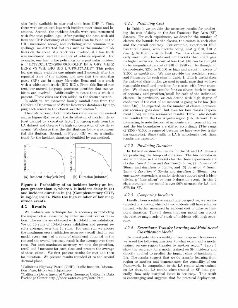
The distribution of both prediction variables is quite skewedand in Figure 4(a) we plot the distribution of incident delay(cost divided by a constant factor) in log-log scale from theLA dataset and observe the high concentration of low delayevents. We observe that the distributions follow a exponen-tial distribution. Second, in Figure 4(b) we see a similartrend for the incident duration identified by our method.
10 1 100 101 102 103
10 2
10 1
100
P(incident delay > x)
Student Version of MATLAB
101 102
10 2
10 1
100
Student Version of MATLAB
P(duration > t)
(a) Incident delay[veh-hrs] (b) Duration [minutes]
Figure 4: Probability of an incident having an im-pact greater than x, where x is incident delay in (a)and incident duration in (b) (Complementary CDF,in log-log scale). Note the high number of low mag-nitude events.
4.2 ResultsWe evaluate our technique for its accuracy in predicting
the impact class, measured by either incident cost or dura-tion. The results are obtained with 10-fold cross validation.We do 10 runs of 10-fold cross validation and present re-sults averaged over the 10 runs. For each run we choosethe maximum cross validation accuracy (recall that in ourmodel every run had a suite of classifiers) obtained in therun and the overall accuracy result is the average over theseruns. For each maximum accuracy, we note the precision,recall and f-measure for each class and present the averageof these values. We first present results for cost and thenfor duration. We present results rounded of to the seconddecimal place.
5California Highway Patrol (CHP) Traffic Incident Informa-tion Page, http://cad.chp.ca.gov6California Department of Water Resources California DataExchange Center,http://cdec.water.ca.gov/intro.html
4.2.1 Predicting CostIn Table 1 we provide the accuracy results for predict-
ing the cost of delay on the San Francisco Bay Area (SF)dataset. For each experiment, we describe the number ofclasses, the bounds for the classes, the counts in each classand the overall accuracy. For example, experiment SF-3has three classes, with buckets being, cost ≤ $10, $10 <cost ≤ $250 and cost > $250. We have chosen semanti-cally meaningful buckets and not buckets that might giveus higher accuracy. A cost of less that $10 can be thoughtto be insignificant, a cost of $10 to $250 can be thought tobe moderate, $250 to $1000 as high and a cost in excess of$1000 as exorbitant. We also provide the precision, recalland f-measure for each class in Table 1. This is useful sincefor a skewed distribution we need to make sure that we havereasonable recall and precision for classes with fewer exam-ples. We obtain good results for two classes both in termsof accuracy and precision/recall for each of the individualclasses. In particular, we can decide with high degree ofconfidence if the cost of an incident is going to be low (lessthan $10). As expected, as the number of classes increases,our accuracy goes down, but even for four classes (experi-ment SF-4) we have reasonable results. Table 1 also detailsthe results from the Los Angeles region (LA) dataset. It isinteresting to note the cost of incidents are in general higherand the bin boundaries are shifted accordingly (The rangeof $250 - $1000 is removed because we have very few train-ing examples). Since traffic in LA is notoriously bad, theseresults are expected.
4.2.2 Predicting DurationIn Table 2 we show the results for the SF and LA datasets
for predicting the temporal duration. The bin boundariesare in minutes, so the buckets for the three experiments are(1) duration ≤ 5min and duration > 5min, (2) duration ≤30min and duration > 30min, and (3) duration ≤ 5min,5min < duration ≤ 30min and duration > 30min. Foremergency responders, a major decision support need is iden-tifying a “false alarm” or near 0 duration event. In this 2class paradigm, our model is over 90% accurate for LA, and87% for SF.
4.2.3 Comparing IncidentsFinally, from a relative magnitude perspective, we are in-
terested in knowing which of two incidents will have a higherimpact, whether measured by incident cost of delay or tem-poral duration. Table 3 shows that our model can predictthe relative magnitude of a pair of incidents with high accu-racy.
4.2.4 Extensions: Transfer Learning and Multi-tieredClassification Model
To investigate the versatility of our proposed frameworkwe asked the following question: to what extent will a modeltrained on one region transfer to another region? Table 4show the accuracy for a model trained on SF incidents anddirectly applied to predict the impact class of incidents inLA. The results suggest that we do transfer learning fromregion to another and demonstrates the versatility of ourframework. In comparison to the LA results when trainedon LA data, the LA results when trained on SF data gen-erally show only marginal losses in accuracy. This resultis encouraging and suggests that for practical deployment,

a) Summary of experimental results for cost
Experiment Classes Bounds ($) Counts AccuracySF-1 2 10 114, 124 95.59SF-2 2 100 157, 81 87.86SF-3 3 10, 250 114,54,70 81.09SF-4 4 10, 250, 1000 114,54,34, 36 73.73LA-1 2 10 75, 97 91.40LA-2 2 250 94,78 88.84LA-3 2 1000 120, 52 82.33LA-4 3 10, 1000 75, 45, 52 75.87
b) Precision, recall and f-measure for cost
Experiment Class Precision Recall f-MeasureSF-1 1 0.95 0.96 0.95
2 0.97 0.95 0.96SF-2 1 0.91 0.91 0.91
2 0.82 0.83 0.821 0.92 0.96 0.94
SF-3 2 0.62 0.55 0.583 0.75 0.76 0.761 0.94 0.96 0.95
SF-4 2 0.61 0.62 0.623 0.51 0.46 0.484 0.47 0.46 0.47
LA-1 1 0.90 0.91 0.902 0.93 0.93 0.92
LA-2 1 0.91 0.88 0.902 0.86 0.89 0.88
LA-3 1 0.87 0.88 0.872 0.72 0.68 0.701 0.87 0.92 0.89
LA-4 2 0.56 0.53 0.553 0.73 0.72 0.72
Table 1: Results for predicting cost. We showedhigh overall accuracy and high precision and recallfor each class.
we will not need to train separate models for each region.The model-building part of this exercise was a bit trickysince CHP in LA and CHP in SF had different “types” forincidents and the distribution of variable values could bedifferent. While we might expect that collecting more dataregarding a particular incident as time passes might improveour prediction, we find no significant improvement in accu-racy in our specific application. One reason might be thatmost incidents are of short duration and for longer durationevents, the first few minutes are not full descriptors of thefull progression of the incident impact. More likely, however,is that we have a limited number of events greater than 15minutes, for example, and thus need more events to get asignificant improvement over the multi-class baseline model.
4.3 DiscussionThe overall classification results are encouraging. In ad-
dition, we discovered models that brought new insights tothe domain experts. For example, the pruned C4.5 treedepicted in Figure 5, which was discovered for predictingfalse alarms in the Los Angeles dataset (70/30 train/test)has over 90% accuracy. The root node of the classificationtree makes a decision based on how different the speed at asensor (two sensors upstream from the incident) is from therecurrent speed. Then, if the speed is significantly below therecurrent speed for that location and time of day, the model
a) Summary of experimental results for duration
Experiment Classes Bounds (min) Counts AccuracySF-1 2 5 146, 92 87.22SF-2 2 30 188, 50 81.05SF-3 3 5, 30 146, 42, 50 72.99LA-1 2 5 85, 87 91.51LA-2 2 30 118, 54 79.65LA-3 3 5, 30 85, 33, 54 71.98
b) Precision, recall and f-measure for duration
Experiment Class Precision Recall f-MeasureSF-1 1 0.89 0.91 0.90
2 0.85 0.82 0.0.83SF-2 1 0.83 0.96 0.89
2 0.63 0.24 0.351 0.92 0.96 0.94
SF-3 2 0.0 0.0 0.03 0.47 0.84 0.61
LA-1 1 0.92 0.91 0.912 0.91 0.92 0.92
LA-2 1 0.95 0.74 0.832 0.62 0.92 0.741 0.91 0.86 0.88
LA-3 2 0.43 0.38 0.403 0.62 0.71 0.66
Table 2: Results for predicting duration of an in-cident. We show high overall accuracies and goodprecision and recall for most experiments.
Measure Region AccuracyCost San Francisco 96.01Cost Los Angeles 94.89
Duration San Francisco 96.3Duration Los Angeles 92.21
Table 3: Prediction accuracy (%) for pairwise rel-ative greater magnitude of incident cost and du-ration. Our model is able to reliably predict therelative magnitude of the impact.
predicts that an accident is occurring. If not, the modelchecks how densely packed the road is. If the road is rela-tively empty, then the model predicts the report as a falsealarm. If not, the model checks to see if any police reportmentioned vehicles involved within the first two minutes. Ifso, the model predicts that an accident is occuring. If not,the model classifies the report as a “false alarm” (meaningthat impact would be negligible). This automatically cre-ated and pruned tree is consistent with intuition and offersinsights, such as that being only k mph slower than recur-rent conditions at a certain time of day and location givenan incident report is a good indicator that it is not a falsealarm. More generally, these models show which variablesare important for prediction.
In addition, our approach is practical and feasible in realtime since both feature extraction and model execution arequick.
As with most data mining problems, when modeling real-world physical systems, having good features is critical. Inthis regard, we found that the features we constructed thatwere trying to imitate the underlying physical models were

Measure Bounds AccuracyCost $10 90.07Cost $10, $100 86.05
Duration 5 Minutes 91.28Duration 5, 30 Minutes 73.84
Table 4: Prediction accuracy (%) by each bin selec-tion choice for k classes of incident delay trained onthe SF dataset and tested directly on LA: the modelresults suggest good transfer learning.
Yes
False alarm
Yes No
No
(v*-‐v)up>4.6
Accident
Yes No
# vehicles>0
Accident False alarm
Figure 5: Classification tree for predicting “falsealarms” for LA, which predicts with >90% accuracyand is consistent with intuition of domain experts.
often good predictors. This might point to a way for con-structing models for physical systems–namely that we lookat some equations from domain experts and capture some ofthose relationships in our feature vectors. Furthermore, inthis work we collected features of different types describing:the incident, changes in the state variable (such as deviationfrom recurrent velocity), the environment (such as rain), andthe topology (refinement is ongoing). We have shown thatthis exercise also improves the accuracy of our models.
Furthermore, for the predicted variable it is importantto first choose a physically useful quantity to predict (suchas the ranges for cost or duration) even at the expense ofaccuracy in models. Making such a choice often causes aproblem with class distribution and makes an already chal-lenging problem even more so. Nevertheless this is neededto get useful models that domain experts want to use.
Our results show that given a cyber-physical system, ma-chine learning techniques can help predict the impact of anincident. We believe that this way of obtaining details ofincidents from some event database, computing impact us-ing sensor data and building a model that correlates the twocan be extended to other domains.
5. CONCLUSIONSIn this paper we have proposed a system for rapid pre-
diction of the cost and impact class of highway incidentsthat demonstrates the real-world applicability of a predictivemodel based on classification models trained on available ur-ban data. The feature vector is built from structured datafrom sensor networks on highways as well as semi-structuredtext collected at different points in time. With experimentson real-world data, we have demonstrated that our modelsare good predictors of incident impact. Thus, our work sup-ports a decision–response to a highway incident–that untilnow has relied on human expertise. In addition to advanc-
ing the use of machine learning for highway operations inpractice, these results open the door to further studies onapplying statistical methods to traffic management and re-lated applications. We are discussing these results with HPServices and a government agency and expect to deploy theunderlying techniques to real-time operations.
6. REFERENCES[1] Valuation of Travel Time in Economic Analysis. Office
of the Secretary of Transportation, U.S. DOT, 2003.
[2] Traffic congestion and reliability : linking solutions toproblems. Federal Highway Administration, 2004.
[3] S. Boyles, S. Boyles, and S. T. Waller. A stochasticdelay prediction model for real-time incidentmanagement, 2007.
[4] C. Chen, Z. Jia, J. Kwon, and E. van Zwet. Statisticalmethods for estimating speed using single-loopdetectors. Submitted to the 82nd Annual Meeting ofthe Transportation Research Board, 2002.
[5] A. Garib, A. E. Radwan, and H. Al-Deek. Estimatingmagnitude and duration of incident delays. Journal ofTransportation Engineering, 123(6):459–466, 1997.
[6] C. Gupta, K. Viswanathan, L. Choudur, M. Hao,U. Dayal, R. Vennelakanti, P. Helm, A. Dev,S. Manjunath, S. Dhulipala, and S. Bellad. Betterdrilling through sensor analytics: a case study in liveoperational intelligence. In Proc. of the 5thInternational Workshop on Knowledge Discovery fromSensor Data, SensorKDD ’11, pages 8–15. ACM, 2011.
[7] C. Gupta, S. Wang, U. Dayal, and A. Mehta.Classification with unknown classes. In M. Winslett,editor, Scientific and Statistical DatabaseManagement, volume 5566 of Lecture Notes inComputer Science, pages 479–496. Springer Berlin /Heidelberg, 2009.
[8] A. Ihler, J. Hutchins, and P. Smyth. Adaptive eventdetection with time-varying poisson processes. InProc. 12th KDD, pages 207–216, New York, NY, USA,2006. ACM.
[9] A. Khattak, X. Wang, and H. Zhang. Incidentmanagement integration tool: dynamically predictingincident durations, secondary incident occurrence andincident delays. Intelligent Transport Systems, IET,6(2):204 –214, 2012.
[10] J. Kwon, M. Mauch, and P. Varaiya. Components ofcongestion: Delay from incidents, special events, laneclosures, weather, potential ramp metering gain, andexcess demand. Transportation Research Record,1959:84–91, 2006.
[11] X. Li, Z. Li, J. Han, and J.-G. Lee. Temporal outlierdetection in vehicle traffic data. In ICDE ’09, pages1319 –1322, 2009.
[12] W. Liu, Y. Zheng, S. Chawla, J. Yuan, and X. Xing.Discovering spatio-temporal causal interactions intraffic data streams. In Proceedings of the 17th ACMSIGKDD international conference on Knowledgediscovery and data mining, KDD ’11, pages1010–1018, New York, NY, USA, 2011. ACM.
[13] A. Skabardonis, P. Varaiya, and K. F. Petty.Measuring recurrent and nonrecurrent trafficcongestion. Transportation Research Record,2003:118–124, 2003.