Ministry of Environment, Notification No. 2010-

Regarding matters about concerning the average fuel efficiency standard for

automobiles, the allowable automobile emission standard of greenhouse gases

(GHGs) for automobiles and application and management of the standards

under Article 47-2 of �Framework Act on Low Carbon, Green Growth� and

Article 37 of Enforcement Ordinance of the Act, the followings are notified.

2010. . .

Minister of Environment

Notification (proposal) about average fuel efficiency standard for

automobiles, allowable emission standard of GHGs for automobiles and

their application and management

Chapter 1. General Provisions

Article 1 (Purpose) The purpose of this Notification is to define the average

fuel efficiency standard and the allowable emission standard of GHGs for

automobiles that automobile manufacturers (including importers, considered

same hereinafter) should follow under Article 47 of �Framework Act on Low

Carbon, Green Growth� and Article 37 of Enforcement Ordinance of the Act

and to stipulate matters necessary to apply and manage the standards.

Article 2 (Terminology) The terms used in this rule are defined as follows:

1. “Fuel efficiency” is a mileage (km/ℓ) per fuel used in automobile.

2. “Average fuel efficiency” is an average (km/ℓ) calculated by dividing the sum

of fuel efficiency of all automobiles sold by auto manufacturers by the number

of automobiles sold.

3. “Average fuel efficiency standard” is a standard (km/ℓ) about the average fuel

efficiency that auto manufacturers should follow.

4. “Greenhouse gas (GHG) emissions” are the sum (g/km) of carbon dioxide

(CO2), methane (CH4) and nitrous oxide (N2O) emitted from an automobile per

mileage.

5. “Average GHG emissions” are the average (g/km) of the sum of GHGs

emitted from all vehicles sold by auto manufacturers by the number of

automobiles sold.

6. “Allowable emission standard of GHGs for automobiles” is the standard

(g/km) about the average GHG emissions that auto manufacturers should

follow.

7. “Same vehicle type” is the group of automobiles whose fuel efficiency and

GHG emissions are expected to be similar according to their structure and

characteristics, and they are not considered as same vehicle type when the

followings are changed:

A. Vehicle type

B. Displacement, supercharger, intake-cooling method, etc.

C. Fuel supply system

D. Transmission type (automatic, manual), gear mode, and drive methods

(front-wheel drive, rear wheel drive, four-wheel drive, etc.)

E. More than 5% of change in complete vehicle curb weight

F. Other cases recognized for their necessity of being separately

categorized

8. “Complete vehicle curb weight” is a total weight of an automobile with a full

tank of fuel, motor oil and coolant, spare tires, standard parts and options

installed on mores than 50% o the vehicles including air conditioner and power

steering wheel that use the power of motor.

Article 3 (Applicable Vehicle) This Notification is applied only to cars and a

van for 10 or fewer passengers sold in Korea, manufactured in Korea or

imported under Article 3 of � Automobile Management Act � and Table 1 in

Article 2 of Enforcement Regulations of the Act and whose total weight is less

than 3.5t, provided that vehicles with the following special purposes are

considered as exception:

1. Vehicles manufactured for the medical purposes such as treatment and

patient transportation.

2. Military vehicles

3. Vehicles manufactured for the purposes of broadcasting,

telecommunication and others

4. Vehicles categorized as special-purpose one considering such purposes

as public interest

Chapter 2. Average fuel efficiency standard and allowable emission

standard of GHGs

Article 4 (Average fuel efficiency standard, allowable emission standard of

GHGs, etc.) � The average fuel efficiency standard for automobiles set by the

Minister of Knowledge Economy and the allowable emission standard of GHGs

for automobiles set by the Minister of Knowledge Economy are described in

Table 1.

�For automobiles to which the average fuel efficiency standard or the

allowable emission standard of GHGs is applied, the rules shall be applied in a

phase-in manner, based upon the sales volume of each auto manufacturer:

30% in 2012; 60% in 2013; 80% in 2014; and 100% in 2015. [

Article 5 (Selection of Standards) � Auto manufacturers should select and

follow either an average fuel efficiency standard or an allowable emission

standard of GHGs every year.

� According to the above �, auto manufacturers should select a standard to

follow for the year and report it to Minister of Environment by end of March. In

this case, if an auto manufacturer wants to change a standard that was selected

for the previous year, it should attach a reason for the standard change. Unless

a car manufacturer additionally submits a standard by end of March, the

manufacturer shall be deemed to keep using the standard selected in the

previous year.

� The Minister of Environment should provide information about standards

selected by auto manufacturers under the above � and � to the Minister of

Knowledge Economy.

� An auto manufacturer, in principle, may not change standards selected for

the year, but unavoidable changes of standard for reasons such as corporate

M&A shall be allowed if the Minister of Environment and the Minister of

Knowledge Economy permit so in consultation

Article 6 (Standard for Manufacturer with Small Sales Volume) In

consultation with the Minister of Knowledge Economy, the Minister of

Environment may define separate rules about standards and application for an

auto manufacturer whose sales volume is small in Korea.

Chapter 3. Measurement of automobile fuel efficiency and GHG emissions

Article 7 (Fuel efficiency and GHG emissions measurement, data

submission, etc.)

� Before putting automobiles on the market, an auto manufacture should

categorize them into a group of the same vehicle type and obtain certification

about fuel efficiency and GHG emissions from the Minister of Environment.

� In order to obtain certification as described in the above �, an auto

manufacturer should have its vehicles measured for fuel efficiency and GHG

emissions by a test agency under Article 9 and submit measurement results

within 30 days in the Appendix No. 1 to the Minister of Environment. When a

auto manufacturer has equipment and personnel approved under �Fuel Use

Rationalization Act � or �Clean Air Conservation Act�, it may test fuel

efficiency and GHG emissions by itself and submit results.

� The Minister of Environment should provide the Minister of Knowledge

Economy with fuel efficiency and GHG emissions information submitted by auto

manufacturers under the above �.

� If certified data such as vehicle fuel efficiency and GHG emissions under

the above � are changed, an auto manufacturer may request change in

certification.

Article 8 (Measurement method of fuel efficiency and GHG emissions) The

methods of measuring vehicle fuel efficiency and GHG emissions are described

in Table 2.

Article 9 (Test agency, etc.) Agencies qualified to measure automobile fuel

efficiency and GHG emissions are entities that have equipment and technical

personnel as described in Table 3 and are as follows:

1. National Institute of Environmental Research

2. Korea Environment Corporation

3. Korea Institute of Fuel Research

4. Korea Automotive Technology Institute

5. Korea Institute of Petroleum Management

6. Other entities that the Minister of Environment permits in consultation with

the Minister of Knowledge Economy

Article 10 (Follow-up) � In its follow-up action, the Minister of Environment

may check whether fuel efficiency and GHG emissions for automobiles are in

line with what have been certified.

� In the follow-up by the Minister of Environment, three vehicles in the same

type from those possessed by an auto manufacturer shall be randomly chosen

and their fuel efficiency and GHG emissions shall be measured by a test

agency under the measurement method of Article 8 in the presence of a

government official designated by the Minister of Environment. However, just

one vehicle is chosen and tested for the same vehicle type if sales volume in

the previous year was fewer than 100.

� If the arithmetic mean values between fuel efficiency and GHG emissions

certified under Article 7 and those measured in the above � exceed the

allowable error tolerance (5%), additional three vehicles should be tested. If the

additionally measured results exceed the allowable error tolerance (5%) again,

the arithmetic mean values measured in the two tests are set as new fuel

efficiency and GHG emissions for the automobile. However, in case of the

same vehicle type in the proviso in the above �, only one additional vehicle is

tested.

Article 11 (Labeling of fuel efficiency and GHG emissions) Auto

manufacturers should label fuel efficiency under Article 15 of � Fuel Use

Rationalization Act � and automobile GHG emissions certified under Article

17 and others.

Chapter 4. Submission and Calculation of Actual Data

Article 12 (Submission of actual data) � Every year, auto manufacturers

should prepare and submit to the Minister of Environment by end of March in

the form of Appendix No. 2 automobile sales volume for the year, fuel efficiency

and GHG emissions data about the same vehicle type, the average fuel

efficiency standard or the allowable emission standard of GHGs for auto

manufacturers to follow and data about emission levels above or below the

standards (“actual data” hereinafter), showing the satisfaction of the average

fuel efficiency standard or the allowable emission standard of GHGs. In such

case, the Minister of Environment should submit actual data from auto

manufacturers to the Minister of Knowledge Economy.

� When the Minister of Environment reviews actual data submitted by a auto

manufacturer under the � and finds nothing incorrect, the Minister should

consult with the Minister of Knowledge Economy the auto manufacturer’s

average fuel efficiency or average GHG emissions for the year,

efficiency/emission levels below or above the standards in actual data or

efficiency/emission levels than can be carried over or should be lowered and

finalize and officially announce them by late June. However, when there is

anything incorrect about actual data submitted by an auto manufacturer, it may

be requested that the manufacturer should correct or complement it and the

manufacturer should submit corrected or complemented actual data to the

Minister of Environment within one month from the request date for correction

or complement

Article 13 (Actual Data Calculation) � Auto manufacturers shall calculate

actual data about average fuel efficiency and average GHG emissions for

automobiles sold for the year as follows, provided that in calculating average

fuel efficiency under the 2 in the below, fuel efficiency certified under Article 7

should be multiplied by 1.26 for the result to be used as fuel efficiency in case

of LPG-powered vehicles.

1. Average GHG emissions (g/km) = [∑(sales volumes of automobiles for

each type (vehicle)× GHG emissions of automobiles for each type (g/km))/ total

sales volume of automobiles (vehicle)]

2. Average fuel efficiency (km/l) = [total sales volume of automobiles

(vehicle)/∑(sales volumes of automobiles for each type (vehicle)/ fuel efficiency

for automobiles of each type (km/l))]

� Auto manufacturers may calculate the average GHG emissions or average

fuel efficiency under the following standards for automobiles emitting low-level

GHGs or with high fuel efficiency.

1. If GHGs emitted by an automobile are less than 50g/km or fuel efficiency

based on fuel type is higher than 46.9km/l for gasoline-powered automobile,

53.8km/l for diesel-powered automobile and 35.3km/l LPG-powered

automobile, every vehicle or electric car that will have been sold each year until

2015 shall be multiplied by three in the calculation.

2. If GHG emitted by an automobiles is ≥50g/km and ≤100g/km or fuel

efficiency based on fuel type is ≥ 23.4km/l and ≤ 46.9km/l for gasoline-powered

automobile, ≥ 26.9km/l and ≤ 53.8km/l for diesel-powered automobile, ≥

17.7km/l and ≤ 35.3km/l for LPG-powered automobile, every vehicle or electric

car that will have been sold in each year until 2015 shall be multiplied by two in

the calculation.

� If technology applied to reduce GHGs and increase fuel efficiency cannot be

measured in test method of Article 8, auto manufacturers may reflect it in

calculating average GHG emissions or average fuel efficiency only when they

can prove the effects of reducing vehicle GHG emissions and increase fuel

efficiency.

� Based on the average consumption efficiency or the average GHG emissions

calculated under the above � to �, auto manufacturers can calculate extra or

insufficient achievement for the year with the following formula. If actual data

meet the standards, it is considered as extra achievement, otherwise as

insufficient achievement.

1. Extra achievement or insufficient achievement in GHGs emissions =

(allowable emission standard of GHGs – average GHG emissions) × sales

volume of automobiles subject to the standard

2. Extra achievement or insufficient achievement in fuel efficiency =

(average fuel efficiency standard – average fuel efficiency) × sales volume of

automobiles subject to the standard

� When an auto manufacturer changes the standards to follow under Article 5,

its actual data shall be estimated again to calculate extra or insufficient

achievement.

Article 14 (Carry-over, trade, etc. of extra achievement) � When an auto

manufacturer has extra achievement, the manufacturer may carry over the

achievement to the next three years from the year of extra achievement or sell

the achievement to other auto manufacturers. However, if the auto

manufacturer has failed to meet the standards for the past three years, extra

achievement should be first used to make up for insufficient achievement.

� An auto manufacturer which is categorized as the one with small volume and

therefore, to which different standards are applied may not trade extra

achievement with other auto manufacturers.

Article 15 (Complement of insufficient achievement) � If an auto

manufacturer fails to achieve the average fuel efficiency standard or the

allowable emission standard of GHGs, first, it should make up for insufficient

achievement within three years from the year of insufficient achievement. In

such case, the auto manufacturer should submit to the Minister of Environment

a plan to do so.

� In order to make up for insufficient achievement, an auto manufacturer may

use its extra achievement carried over or buy extra achievement from other

manufacturers.

Supplementary Provisions

This Notification takes effect from January 1st, 2012.

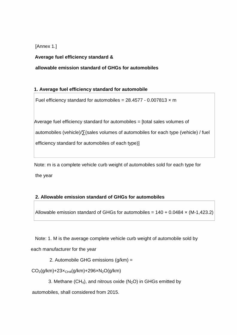
[Annex 1.]

Average fuel efficiency standard &

allowable emission standard of GHGs for automobiles

1. Average fuel efficiency standard for automobile

Fuel efficiency standard for automobiles = 28.4577 - 0.007813 × m

Average fuel efficiency standard for automobiles = [total sales volumes of

automobiles (vehicle)/∑(sales volumes of automobiles for each type (vehicle) / fuel

efficiency standard for automobiles of each type)]

Note: m is a complete vehicle curb weight of automobiles sold for each type for

the year

2. Allowable emission standard of GHGs for automobiles

Allowable emission standard of GHGs for automobiles = 140 + 0.0484 × (M-1,423.2)

Note: 1. M is the average complete vehicle curb weight of automobile sold by

each manufacturer for the year

2. Automobile GHG emissions (g/km) =

CO2(g/km)+23×CH4(g/km)+296×N2O(g/km)

3. Methane (CH4), and nitrous oxide (N2O) in GHGs emitted by

automobiles, shall considered from 2015.

[Annex 2]

Vehicle energy consumption efficiency and greenhouse gas emissions

measurement method

� To measure vehicle energy consumption efficiency and greenhouse gas emissions,

use the combined mode that consists of the CVS-75 (city drive) mode and the

Highway (highway drive) mode.

� Calculate energy consumption efficiency and greenhouse gas emissions measured

in the combined mode as follows:

- Vehicle energy consumption efficiency (km/L) = 1/[0.55/fuel efficiency measured in

the CVS-75 mode (km/L) + 0.45/ fuel efficiency measured in the Highway mode (km/L)]

- Vehicle greenhouse gas emissions (g/km) = 0.55* greenhouse gas emissions

measured in the CVS-75 mode (g/km) + 0.45* greenhouse gas emissions measured in

the Highway mode (g/km)

� Measurement in CVS-75 mode (relevant to Article 7)

1. Device

A device to measure vehicle energy consumption efficiency and greenhouse gas

emissions consists of a chassis dynamometer, an exhaust gas sampler, an exhaust

gas analyzer, a data-processing unit and other parts.

A. Gasoline and gas-powered vehicle

(1) Chassis dynamometer

(A) It should be possible to use a load absorption unit to reproduce road driving

conditions and use methods including a flywheel method to reproduce an inertia

weight.

(B) There should be a RPM counter for a roll or an axis, or it should be possible to

measure mileage in any other methods recognized by the Minister of

Environment.

(C) The diameter of a nominal roll consisting of two small rolls should be 22cm

(17in). And the diameter of a single roll in a dynamometer should be 122cm (48in).

A dynamometer with a roll of a different diameter may be used if same road load

can be reproduced and the Minister of Environment recognizes it better.

(2) Sampler

(A) Overview

It should be designed to measure actual vehicle gas emissions (Figure 1). A

certain flow should be continuously collected from a sample. Emissions are

calculated from a sample concentration and a total flow during the test.

(B) Device requirement

A critical flow venturi-constant volume sampling (CFV-CVS) is widely used and

other samplers, if approved in advance by the Minister of Environment, may be

used.

1) Change in constant pressure in vehicle vent pipe: When nothing is connected

to a vent pipe, the constant pressure should be within ±127mm H2O (1.2kpa) in

one driving cycle of a dynamometer.

2) Accuracy and precision of thermometer: The temperature should be within

±1.1� (2�) and it should be possible to read 62.5% of a temperature change

within 0.100 sec. in terms of sensitive time.

3) Accuracy and precision of pressure measurement device: ±40mmH2O(0.4

kpa)

4) CVS flow: It should be sufficient to prevent moisture condensation. (In most

vehicles, 0.140-0.165m3/sec (300 - 350cfm) would be sufficient.)

5) Sampling pouch: It should be big enough not to prevent the flow of a sample.

(3) Exhaust gas analyzer

(A) NOx analyzer: Use a chemical luminescence method (CLD).

(B) CO and CO2 analyzer: Use a non-dispersive infrared analyzer (NDIR).

(C) HC analyzer: Use Flame Ionization Detector (FID) as an HC (total

hydrocarbon) analyzer. Ise Gas Chromatography-FID (GC-FID) or its equivalent or

higher level as CH4 (methane) analyzer.

[Figure 1] Exhaust gas sampler (CFV - CVS)

B. Diesel-powered vehicle

(1) Overview

It is intended to measure gas emissions from a diesel-powered vehicle by the CVS

method in the same approach as in a gasoline-powered vehicle. And to measure

hydrocarbon (HC), directly collect it from a diluted sample and measure it with

heated FID (HFID).

(2) Device requirements

(A) CFV-CVS requirements for a diesel-powered vehicle are same with those in a

gasoline-powered vehicle except the followings:

1) There should be a heat exchanger.

2) The temperature of the diluted emission gas measured right before CFV

should be within ±11�(20�) from the temperature set at the start of the

measurement. And the accuracy and precision of the thermometer should be

within ±1.1�(2�).

(B) To minimize heat loss in exhaust gas, a pipe connecting a vent pipe and a

dilution tunnel should be made of stainless steel at 610cm(20ft), if warmed, or

365cm(12ft)m if not warmed.

(C) The temperature of the diluted air should be 20-30�(68-86�) at the time of

measurement.

(D) Dilution tunnel

1) A heated hydrocarbon sampling tube should be prepared in a way to collect

sufficiently mixed gas.

2) Its diameter should be at least 20.3Cm (8.0in).

3) It should be electrically conductive that does not react with exhaust gas

composition.

4) It should be earthed.

(E) The internal temperature of a dilution tunnel should be high enough to prevent

moisture condensation but should not be higher than 52� (125�) from a sampling

point during measurement.

(F) Sampling tube for hydrocarbon measurement

1) It should be placed where diluted air and exhaust can be mixed enough.

2) The temperature should be maintained at 191±11� (375±20�).

4) Its internal diameter should be at least 0.457cm (0.19").

(G) The degree of a temperature detector should be within ±1.1� (±2�).

(H) Diluted exhaust gas flow in sampler for hydrocarbon measurement

1) The temperature inside a heating device should be 191±6�(375±10�) and

temperature detector degree should be ±1.1�(2�).

2) The temperature of diluted exhaust gas in a hydrocarbon measurement

device should be 185-197�(365-385�).

(I) An exhaust gas analyzer is all same with that for a gasoline-powered vehicle

except a hydrocarbon analyzer.

2. Measurement of exhaust gas

During the test, the laboratory temperature should be kept at 20-30�(68-86�).

A. Test vehicle preparation and preliminary drive

(1) Before testing, drive a vehicle at mileage (breaking in) of more than 3,000km

under durability driving schedule in � Clean Air Conservation Act � or its equivalent

schedule. However, the breaking-in may be omitted or shortened when energy

consumption efficiency and greenhouse gas emissions are checked for a follow-up test

vehicle as described in Article 10.

(2) Conduct mechanical inspection according to the vehicle specifications.

(3) Check fuel quantity in fuel tank. (Inject defined test fuel more than 40%.)

(4) Place a test vehicle onto a chassis dynamometer and drive it under Urban

Dynamometer Driving Schedule (UDDS).

(5) Remove the vehicle from a dynamometer in 5 minutes after the completion of

preliminary drive, and move it to a parking space to park it. The parking hour is 12 to 36

hours for a gasoline or gas-powered vehicle and more than 12 hours for a

diesel-powered vehicle.

B. Exhaust gas measurement

On a dynamometer, drive a test vehicle in the following three stages and collect and

analyze exhaust gas at each stage.

Stage Time (sec.) Distance Note Cold running test Initial stage Cold running test Stable stage Parking High running test

505 865 9-11 min. 505

5.78km (3.59 mile) 6.29km (3.91 mile) - 5.78km (3.59 mile)

Start at low temperature Start at high temperature

Total 44 min. 17.85km (11.59 mile)

(1) Sequence of exhaust gas measurement

(A) Push a vehicle onto a dynamometer, without starting the engine.

(B) Open the hood and place a cooling fan 30.5cm (12in) in front of the chassis.

(C) Connect a test sampling valve to a sampling pouch in vacuum to collect diluted

exhaust and diluted air.

(D) Run CVS, a sampling pump, a temperature recorder and a vehicle cooling fan.

(E) Adjust a sampling flow to the defined one and set the gas flow measurement

device to zero.

1) The minimum flow of gas sample (except hydrocarbon) is 0.08l/sec(0.17cfm).

2) The minimum flow of hydrocarbon sample is 0.031l/sec (0.067cfm).

(F) Connect an exhaust sampling tube to a vehicle vent pipe.

(G) Run the gas flow measurement device, and direct the sample gas flow over

the sample selection valve toward exhaust sample pouch during “initial stage of

cold running test” and toward diluted air pouch during “initial stage of cold running

test”. In case of a diesel-powered vehicle, run the integrator of hydrocarbon

analyzer.

(H) Shift the gear 15 sec. after starting the engine.

(I) Initially accelerate the vehicle 20 sec. after starting the engine under the driving

schedule.

(J) Drive the vehicle under urban dynamometer driving schedule (UDDS).

(K) After driving the vehicle for 505 sec., decelerate it. Then, immediately change

the sample flow from the pouch at the initial stage of cold running test to the pouch

at the stable stage of cold running test, and stop No. 1 of the gas flow

measurement device.

(L) Run No. 2 of the gas flow measurement device. In case of a diesel-powered

vehicle, run No. 2 of the diesel hydrocarbon integrator.

(M) Record RPM of a roller or an axis before the acceleration that starts 510th sec.

and set the counter to zero or replace it with the second counter.

(N) Send exhaust sample and diluted air at the initial stage of cold running test to

the analyzer as soon as possible and analyze them in 20 minutes from sampling

under the exhaust gas analysis method to get stable analysis results.

(O) Stop the engine 2 sec. after final deceleration of 1369 sec.

(P) After 5 sec. when the engine is stopped, turn off No. 2 of the gas flow

measurement device

(Q) Set the sample selection valve to “Preparation”.

(R) Record RPM of a roller or an axis and the value on gas meter or flow meter

and then set the counter back.

(S) Send exhaust gas and diluted air sample at the initial stage of cold running

test to the analyzer as soon as possible and analyze them in 20 minutes from

sampling to get stable analysis results.

(T) Turn off the cooling pan immediately after sampling.

(U) Turn off CVS, or separate exhaust gas sampling tube from a vehicle vent pipe.

(V) For high running test, repeat (B) to (K). Start operation in (H) between 9 and

11 min. after sampling for cold start is done.

(W) After driving the vehicle for 505 sec. decelerate it. Then, immediate turn off

No. 3 of the gas flow measurement device. In case of a diesel-powered vehicle,

set a sample selection valve to “Preparation”. Record RPM of a roller axis and

also record a No. 3 gas meter value and a flow value measured.

(X) Send exhaust and diluted air “at the initial stage of hot running test” to an

analyzer as soon as possible to analyze them in 20 min from sampling.

(Y) Separate a sampling tube from a vehicle vent pipe and move the vehicle from

dynamometer to a sealed room. It is accepted to move it by driving.

(Z) Turn off CVS and CFV.

(2) Exhaust analysis

(A) CO, CO2, NOx, HC and CH4 analysis

1) Set an analyzer to zero to get a stable value and inspect the device after test.

2) Send span gas to calibrate gain on analyzer. To reduce error, set the span

value at the same flow with the one used to measure a sample and calibrate it.

Use the span gas with the 75-100% of full-scale concentration. If gain on

analyzer gives big impact, check calibration and record accrual concentration of

record note.

3) Check the zero and if necessary, repeat 1) and 2).

4) Check flow and pressure.

5) Measure CO, CO2, NOx, HC and CH4 concentrations of sample.

6) Check the zero and a span value. If a variance is bigger than 2% of full scale,

repeat (A)-(B).

(B) Diesel hydrocarbon analysis

1) Calibrate the zero of a HFID analyzer and get stable zero.

2) Send span gas to calibrate gain on analyzer. Use the span gas with the

75-100% of full-scale concentration.

3) Check the zero. Zero gas and span gas in the analyzer can be adopted in any

one of the following methods:

A) Close an HC sample heat valve and let gas flow into HFID.

B) Directly connect the zero and span gas tube to HC sample tube, and let the

gas at 190-210% HFID flow.

Note: To minimize error, make HFID flow and pressure same at the time of

zero span calibration and measurement.

4) During measurement, continuously record the exhaust concentration of

diluted hydrocarbon.

5) Check the zero point and a span value. If the variance is bigger than 2% of

full scale, stop the test and check HC “hang-up” or electric “drift” of an

analyzer.

(3) Exhaust calculation

(A) Ywm = 0.43[Yct + Ys)/(Dct + Ds)] + 0.57[(Yht + Ys)/(Dht + Ds)]

Here,

Ywm = CO, CO2, NOx, HC, CH4 and NMHC weighted exhaust gas mass

(g/km, g/mile)

Yct = exhaust gas mass at the initial stage of cold running test (g/test

step)

Yht = exhaust gas mass at the initial stage of hot running test (g/test

stage)

Ys = exhaust gas mass at the stable stage of cold running test (g/test stage)

Dct = mileage at the initial stage of cold running test (km, mile)

Dh = Mileage at the initial stage of hot running test (km, mile)

Ds = Mileage at stable stage of cold running test (km, mile)

(B) Mass concentration of pollutants by stage in driving test

HCmass = Vmix x HC density x (HCconc/106)

CH4mass = Vmix x CH4 density x (CH4conc/106)

NMHCmass = Vmix x NMHC density x (NMHCconc/106)

NOxmass = Vmix x NO2 density x (NOxconc/106)

COmass = Vmix x CO density x (COconc/106)

CO2mass = Vmix x CO2 density x (CO2conc/102)

Here,

HCmass = hydrocarbon mass concentration (g/test stage)

HCdensity = 0.5768kg/m3 (16.33g/ft3) (ratio of carbon to hydrogen at

1:1.85 and at 20�101.3Kpa 68� 760mmHg)

HCconc = hydrocarbon concentration in diluted exhaust whose hydrocarbon

concentration is adjusted in diluted air (ppmC)

HCconc = HCe - HCd (1-1/DF)

Here,

HCe : hydrocarbon concentration in diluted exhaust (ppmC)

HCd : hydrocarbon concentration in diluted air (ppmC)

CH4mass = CH4 mass concentration (g/test stage)

CH4density = 0.6672kg/m3 (18.89g/ft3) (20�, 101.3Kpa(at 68�,

760mmHg))

CH4conc = CH4 concentration in diluted exhaust whose CH4 concentration is

adjusted in diluted exhaust (ppmC)

CH4conc = CH4e - CH4d(1-1/DF)

Here,

CH4e = CH4 concentration in diluted exhaust (ppmC)

CH4d = CH4 concentration in diluted air (ppmC)

NMHCmass = NMHC mass concentration (g/test stage)

NMHCdensity = 0.5768kg/m3 (gasoline, diesel) and 0.04157(12.011 +

H/C(1.008))kg/m3(natural gas, LPG) (at 20�, 101.3Kpa (at 68�, 760mmHg))

Here,

H/C = ratio of carbon to hydrogen of test fuel

NMHCconc = NMHC concentration in diluted exhaust whose NMHC

concentration is adjusted in diluted air (ppmC)

NMHCconc = HCconc - (rCH4 × CH4conc)

Here,

rCH4 = FID response factor for methane, in case of a natural gas-powered

vehicle

rCH4 = FIDppm / SAM ppm

Here,

FID ppm : methane concentration(ppmC) analyzed in FID,

SAM ppm: known methane concentration (ppmC), rCH4=1 for other

vehicle

NOxmass = nitrogen oxide mass concentration(g/test stage)

NO2density = 1.913kg/m3 (54.16g/ft3)(20�, 101.3Kpa(NO2 at 68�

760mmHg))

NOxconc = NOx concentration in diluted exhaust whose NOx

concentration is adjusted in diluted air (ppm)

NOxconc = NOxe - NOxd(1-1/DF)

Here,

NOxe = NOx concentration in dilute exhaust (ppm)

NOxd = NOx concentration in diluted air (ppm)

COmass = carbon monoxide mass concentration (g/test stage)

COdensity = 1.164kg/m3(32.97g/ft3) (20�, 101.3Kpa (68� 760mmHg))

COconc = CO concentration in diluted exhaust whose CO concentration

is adjusted in diluted air (ppm)

COconc = COe - COd(1-1/DF)

Here,

COe : CO concentration in diluted exhaust adjusted by water vapor

pressure and CO2 extraction (ppm), ratio of C to H assumed at 1:1.85

COe = (1-0.01925 CO2e - 0.000323 R) COem

COd : CO concentration in diluted exhaust adjusted by water vapor

pressure extraction (ppm)

COd = (1 - 0.000323 R) × COdm

R : relative humidity in diluted air (%)

COem : CO concentration in diluted exhaust (ppm)

COdm : CO concentration in diluted air sample (ppm)

CO2mass : carbon dioxide mass concentration(g/test stage)

CO2density = 1.830kg/m3(51.81g/ft3)(20�, 101Kpa (68� 760mmHg))

CO2conc = 1

CO2conc = CO2e - CO2d(1-1/DF)

Here,

CO2e : CO2 concentration in diluted exhaust (%)

CO2d : CO2 concentration in diluted air (%)

DF = 13.4/[CO2e + (HCe + COe)10-4)

KH = humidity adjustment factor

KH = 1/[1-0.0047(H-75)] or KH = 1/[1-0.0329 (H-10.71)] (in SI unit)

Here,

H = absolute humidity (H2O grain/1b dry air, gH2O/kg dry air)

H = [(6.211)Ra x Pd]/[Pb - (Pd x Ra/100)]

H = [(43.478)Ra x Pd]/[Pa - (Pd x Ra/100)] (in SI unit)

Ra = relative humidity in the atmosphere (%)

Pd = saturated water vapor pressure at dry-bulb temperature in the

atmosphere (mmHg, kPa)

Pb = air pressure (mmHg, kPa)

Vmix = total diluted exhaust adjusted by the standard conditions (293K,

101.3Kpa(528R 760mmHg) (m3/test stage or ft3/test stage)

3. Test fuel

A. Use the test fuels of gasoline, gas and diesel that satisfy the requirements in

� Clean Air Conservation Act � and � Petroleum Business Act �. Diesel used in the

test should be pure and clean whose pure point and cloud point should be appropriate

to driving, and may contain Cetane number enhancer, metal deactivator, antioxidant,

anticorrosive agent, pure point inhibitor, and nonmetallic additives such as pigment and

dispersing agent.

B. A different test fuel may be used if a manufacturer determines there is no impact

on test results.

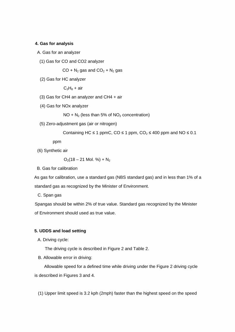
4. Gas for analysis

A. Gas for an analyzer

(1) Gas for CO and CO2 analyzer

CO + N2 gas and CO2 + N2 gas

(2) Gas for HC analyzer

C3H8 + air

(3) Gas for CH4 an analyzer and CH4 + air

(4) Gas for NOx analyzer

NO + N2 (less than 5% of NO2 concentration)

(5) Zero-adjustment gas (air or nitrogen)

Containing HC ≤ 1 ppmC, CO ≤ 1 ppm, CO2 ≤ 400 ppm and NO ≤ 0.1

ppm

(6) Synthetic air

O2(18 – 21 Mol. %) + N2

B. Gas for calibration

As gas for calibration, use a standard gas (NBS standard gas) and in less than 1% of a

standard gas as recognized by the Minister of Environment.

C. Span gas

Spangas should be within 2% of true value. Standard gas recognized by the Minister

of Environment should used as true value.

5. UDDS and load setting

A. Driving cycle:

The driving cycle is described in Figure 2 and Table 2.

B. Allowable error in driving:

Allowable speed for a defined time while driving under the Figure 2 driving cycle

is described in Figures 3 and 4.

(1) Upper limit speed is 3.2 kph (2mph) faster than the highest speed on the speed

curve in less than 1 sec. of defined time

(2) Lower limit speed is 3.2 kph (2mph) slower than the lowest speed on the speed

curve in less than 1 sec. of defined time.

(3) Speed change bigger than allowable error at times such as gear shift is accepted

if it occurs within 2 sec.

(4) If a vehicle is running on maximum horsepower, a speed lower than the above

descriptions is accepted.

(5) Upper and lower limit speed during warming up driving is 6.4kph (4mph).

C. transmission

(1) Unless explained otherwise, all test conditions should be prepared as per the

recommendations by a manufacturer given to a final consumer.

(2) For automatic transmission, set the idle mode into “Drive (D)" condition and set

wheels into the brake mode. For manual transmission, put off the clutch and shift a

gear to drive except the initial idle mode.

(3) Softly accelerate under the instructed transmission procedure. In manual

transmission, a driver should take the foot off the accelerator at each transmission

and shift the gear in a short time. If a vehicle does not accelerate to a defined speed,

drive it to exert maximum power until it reaches the speed defined under the driving

schedule.

(4) In the deceleration mode, use a brake or an accelerator, if necessary, to maintain

required speed, and drive a vehicle with gear shifted. For a vehicle with manual

transmission, a gear should not be shifted from a previous mode after the clutch is

connected. During deceleration to the zero, step on the clutch if the speed drops to

lower than 24.1kph (15mph), an engine is unstable, or an engine is about to stop.

[Figure 2] Dynamometer driving cycle

[Table 2]

[Figure 3] Driving volume, acceptable range

[Figure 4] Driving volume, acceptable range

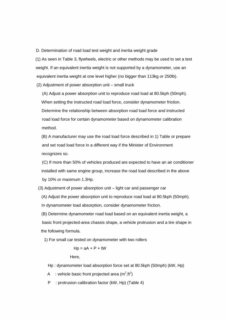
D. Determination of road load test weight and inertia weight grade

(1) As seen in Table 3, flywheels, electric or other methods may be used to set a test

weight. If an equivalent inertia weight is not supported by a dynamometer, use an

equivalent inertia weight at one level higher (no bigger than 113kg or 250lb).

(2) Adjustment of power absorption unit – small truck

(A) Adjust a power absorption unit to reproduce road load at 80.5kph (50mph).

When setting the instructed road load force, consider dynamometer friction.

Determine the relationship between absorption road load force and instructed

road load force for certain dynamometer based on dynamometer calibration

method.

(B) A manufacturer may use the road load force described in 1) Table or prepare

and set road load force in a different way if the Minister of Environment

recognizes so.

(C) If more than 50% of vehicles produced are expected to have an air conditioner

installed with same engine group, increase the road load described in the above

by 10% or maximum 1.3Hp.

(3) Adjustment of power absorption unit – light car and passenger car

(A) Adjust the power absorption unit to reproduce road load at 80.5kph (50mph).

In dynamometer load absorption, consider dynamometer friction.

(B) Determine dynamometer road load based on an equivalent inertia weight, a

basic front projected-area chassis shape, a vehicle protrusion and a tire shape in

the following formula.

1) For small car tested on dynamometer with two rollers

Hp = aA + P + tW

Here,

Hp : dynamometer load absorption force set at 80.5kph (50mph) (kW, Hp)

A : vehicle basic front projected area (m2,ft2)

P : protrusion calibration factor (kW, Hp) (Table 4)

W : vehicle equivalent inertia weight in Table 3 (Kg,lb)

a : 3.452(hatch back style), 4.013 (others)

t : 0.0 for a vehicle with radial tires, 4.93 x 10 for others

Definition of hatch back style: The orthogonal projection at the rear of a vehicle

has less than 20o degree on the plane takes up more than 25% of front projected

area. The surface should be smooth and continuous with no partial change of

more than 4o. The example of a hatch-back style is in Figure 5.

AP, the front projected area of the protrusion, is defined in the same way with the

front projected area of a vehicle. In other words, it is the entire orthogonal

projection area of mirror, hood ornament, roof rack, and other protrusions on the

plane rectangular to each side of a vehicle and on the plane of a vehicle.

protrusion refers to a fixture that is installed at more than 2.54cm(1 in) from the

vehicle and whose projected area is more than 0.0093m3(0.01ft3) by the

calculation approved in advance by the Minister of Environment. The entire front

projected area of protrusion should include all of standard outfit. If there is any

option expected to be installed in more than 50% of vehicle selected, it also

should be included.

2) In case of light car and passenger car, round off power absorption setting

value of vehicle dynamometer to 0.07kW (0.1 Hp).

3) For light car and passenger car tested on vehicle dynamometer with one big

roller,

HP = aA + P + (8.22 x 10-4 + 0.33t)W

HP = 0.746kW

Round off all symbols and numbers in the above formula to one decimal

place.

[Table 3] Equivalent inertia weight of road load

Loaded vehicle weight Equivalent inertia weight Inertia weight 80.5kph

highway load (small truck) Note 1,2,3

kg ℓb kg ℓb kg ℓb

481.8 481.9-538.5 538.6-595.2 595.3-651.9 652.0-708.6 708.7-765.3 765.4-822.0 822.1-878.7 878.8-935.4 935.5-992.1 992.2-1048.8

1048.9-1105.5 1105.6-1162.2 1162.3-1218.9

1,062 1,063-1,187 1,188-1,312 1,313-1,437 1,438-1,562 1,563-1,687 1,688-1,812 1,813-1,937 1,938-2,062 2,063-2,187 2,188-2,312 2,313-2,437 2,438-2,562 2,563-2,687

453.6 510.3 567.0 623.7 680.4 737.1 793.8 850.5 907.2 963.9 1,020.6 1,077.3 1,134.0 1,190.7

1,000 1,125 1,250 1,375 1,500 1,625 1,750 1,875 2,000 2,125 2,250 2,375 2,500 2,625

453.6 453.6 567.0 567.0 680.4 680.4 793.8 793.8 907.2 907.2 1,020.6 1,020.6 1,134.0 1,134.0

1,000 1,000 1,250 1,250 1,500 1,500 1,750 1,750 2,000 2,000 2,250 2,250 2,500 2,500

1219.0-1275.6 1275.7-1332.3 1332.4-1389.0 1389.1-1445.7 1445.8-1502.4 1502.5-1559.1 1559.2-1615.8 1615.9-1672.5 1672.6-1729.2 1729.3-1785.9 1786.0-1871.2 1871.3-1984.6 1984.7-2098.0 2098.2-2211.4

2,688-2,812 2,813-2,937 2,938-3,062 3,063-3,187 3,188-3,312 3,313-3,437 3,438-3,562 3,563-3,687 3,688-3,812 3,813-3,937 3,938-4,125 4,126-4,375 4,376-4,625 4,626-4,875

1,247.4 1,304.1 1,360.8 1,417.5 1,474.2 1,530.9 1,587.6 1,644.3 1,701.0 1,757.7 1,814.4 1,927.8 2,041.2 2,154.6

2,750 2,875 3,000 3,125 3,250 3,375 3,500 3,625 3,750 3,875 4,000 4,250 4,500 4,750

1,247.4 1,247.4 1,360.8 1,360.8 1,360.8 1,587.6 1,587.6 1,587.6 1,587.6 1,814.4 1,814.4 1,814.4 2,041.2 2,041.2

2,750 2,750 3,000 3,000 3,000 3,500 3,500 3,500 3,500 4,000 4,000 4,000 4,500 4,500

2,211.5-2,324.8 2,324.9-2,438.2 2,438.3-2,608.3 2,608.4-2,835.1

2,835.2-3,061.9 3,062.0-3,288.7 3,288.8-3,515.5 3,515.6-3,742.3 3,742.4-3,969.1 3,969.2-4,195.9 4,196.0-4,422.6 4,422.7-4,535.9

4,876-5,125 5,126-5,375 5,376-5,750 5,751-5,250 6,251-6,750 6,751-7,250 7,251-7,750 7,751-8,250 8,251-8,750 8,751-9,250 9,251-9,750 9,751-10,000

2,268.0 2,381.4 2,494.8 2,721.6 (Note 4) 2,948.3 3,175.1 3,401.9 3,628.7 3,855.5 4,082.3 4,309.1 4,535.9

5,000 5,250 5,500 6,000

6,500 7,000 7,500 8,000 8,500 9,000 9,500

10,000

2,268.0 2,268.0 2,494.8 2,721.6

2,948.3 3,175.1 3,401.9 3,628.7 3,855.5 4,082.3 4,309.1 4,535.9

5,000 5,000 5,500 6,000

6,500 7,000 7,500 8,000 8,500 9,000 9,500

10,000

Note)

1. For a small truck except a van-style car and a heavy duty vehicle

exceptionally recognized as a small truck, calculate the road load at 80.5kph

by multiplying B (as defined in the below 3) rounded off by every

0.4km(0.5HP) by 0.58.

2. For a van-style vehicle, calculate the road load at 80.5kph by multiplying B

(as defined in the below 3) rounded off by every 0.4kw (0.5HP) by 0.5.

3. “B" is the sum of a basic vehicle front area (� ) and a front area that

exceeds 0.009 � because of mirror and others options expected to be sold

more than 50% of vehicle type. Calculate the front area to the five decimal

points of � by using a method approved in advance by the Minister of

Environment.

4. For a light vehicle whose loaded weight exceeds 2,608kg(5,750lb), test it

with the equivalent test weight of 2,495kg(5,500lb) and the road load force of

10.7kw (14.4HP).

[Table 4] Protrusion horsepower calibration factor

Ap( � ) Area P : kw (horsepower)

Ap � 0.02787 ............................................................

0.02787≤Ap � 0.05574 ........................................

0.05574≤Ap � 0.08361 ........................................

0.08361≤Ap � 0.11148 ........................................

0.11148≤Ap � 0.13935 ........................................

0.13935≤Ap � 0.16722 ........................................

0.16722≤Ap � 0.19509 ........................................

0.19509≤Ap � 0.22296 ........................................

0.22296≤Ap � 0.25083 ........................................

0.25083≤Ap � 0.2787 ..........................................

0.2787≤Ap ..............................................................

0.0 (0.0 )

0.30(0.40)

0.52(0.70)

0.75(1.00)

0.97(1.30)

1.19(1.60)

1.42(1.90)

1.64(2.20)

1.86(2.50)

2.09(2.80)

2.31(3.10)

[Figure 5] Hatch back style example

(C) When more than 50% of vehicles with the same device group are expected to

have air conditioner installed, and such vehicles are tested, increase the road load

determined in 2) and the road load in Table of 1) by 10% or to a maximum 1kW

(1.3Hp). Such increase for an air conditioner should be done before rounding off

as instructed in Note 2 and 3 of Table 6. However, this is not applied when the test

is done on the chassis dynamometer with one big roller.

(D) A manufacturer may calculate the road load as in the above way or determine

the road load by using another method approved in advance by the Minister of

Environment.

6. Device calibration

A. Since device calibration could have critical impact on a device or exhaust gas

composition, calibrate it on a regular basis after maintenance as follows:

(1) Monthly inspection

(A) Analyzer calibration: CO, CO2, HHC, NOx, HC, and CH4 analyzer

(B) Chassis dynamometer calibration

(2) Weekly inspection

(A) NOx converter efficiency

(B) CVS inspection

(C) Dynamometer performance test

B. Calibration method of device

(1) Calibration method of chassis dynamometer device, etc.

(A) Calibration method of chassis dynamometer

There are two calibration methods of dynamometer: calibration under calibration

procedure recommended by a dynamometer manufacturer and a method of

measuring dynamometer frictional force absorption at 80.5kph (50mph). Another

method may be used if dynamometer frictional force absorption can be measured.

Measured absorption road load means the load absorbed by a load absorption

unit. In terms of dynamometer frictional force on a dynamometer, after running a

dynamometer at 80.5kph (50mph), remove a device used to run the dynamometer

from the dynamometer to coast down a roller speed. At this time, kinetic energy of

the device is consumed by the dynamometer. This method ignores the change

from roller bearing friction that arises from a vehicle driving axis weight. And if a

dynamometer with two rollers is used, it is acceptable to ignore the inertia of a free

roller (rear roller).

1) Measure a speed of a driving roller, if not previously measured. At this time,

use five wheels, RPM counter or any other appropriate method.

2) Place a vehicle onto a dynamometer or install a device that can run the

dynamometer in a different way.

3) Install flywheels with a inertia weight in the range of most general vehicle

weights used in dynamometer or a different inertia mass device.

4) Run dynamometer up to 80.5kph (50mph).

5) Record shown road load.

6) Run the dynamometer up to 96.9kph (60.0mph).

7) Remove a device used to run the dynamometer.

8) Record the time taken to decelerate a driving roller of the dynamometer from

88.5kph (55mph) to 72.4kph (45mph).

9) Adjust a power absorption unit to another level.

10) Repeat (D)-(I) in the above to include the range of road load being used.

11) Calculate absorption road load (HPd)

HPd = (1/2) (W/9.807)(V1 - V2 )/102t

Here, HPd : load force (kw,Hp)

W : equivalent inertia weight (kg,lb)

V1 : initial speed (m/s,ft/s)

V2 : final speed (m/s,ft/s)

t : time taken for a roller to decelerate from

88.5kph(55mph) to 72.4kph(45mph)

To simply the above formula,

HPd : 0.06073(w/t) (in English unit)

HPd : 0.09984(w/t)(in SI unit)

12) Draw the relationship diagram between instructed road load force and actual

road load force at 80.5kph (50mph) in Figure 6.

[Figure 6] actual/marked road load

(B) Chassis dynamometer performance test

Do a coast down test of chassis dynamometer in one or more inertia-horse power

setting and compare the result with the coast time acquired in recent calibration. If

a variance is bigger than 1 sec., calibrate it again.

(C) CVS calibration method

1) Calibration method

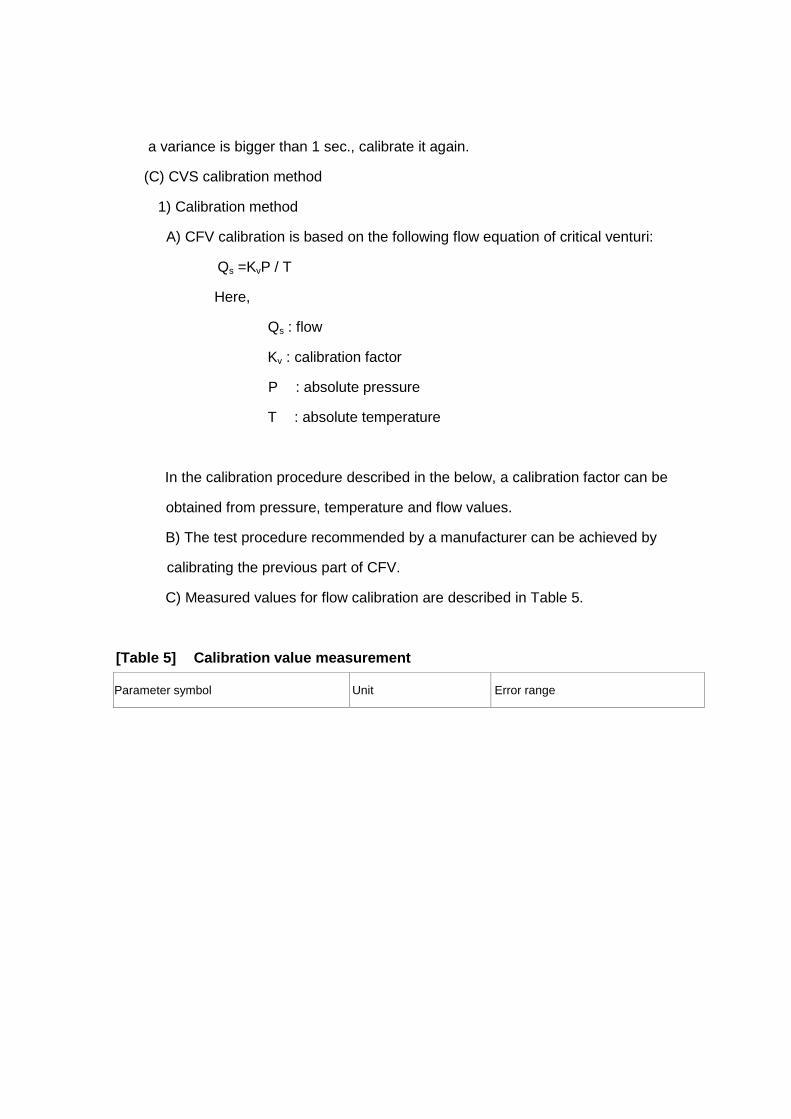
A) CFV calibration is based on the following flow equation of critical venturi:

Qs =KvP / T

Here,

Qs : flow

Kv : calibration factor

P : absolute pressure

T : absolute temperature

In the calibration procedure described in the below, a calibration factor can be

obtained from pressure, temperature and flow values.

B) The test procedure recommended by a manufacturer can be achieved by

calibrating the previous part of CFV.

C) Measured values for flow calibration are described in Table 5.

[Table 5] Calibration value measurement

Parameter symbol Unit Error range

Pressured (modified) ................ Pb

Air temperature, flow meter...... ETI

LFE upstream pressure decrease..... EPI

LFE mattress pressure

increase................................. EDP

Air flow ......................... Qs

Pressure decrease at CFV inlet.. PPI

Temperature at Venturi,

Inlet.................................. Tv

Proportion in mano meter flow

(1.75 Oil) ................... SP.GR

KPa(in, Hg)

�(F)

KPa(inH20)

KPa(inH20)

� /min(ft3/min)

KPa(in, fluid)

�(F)

±0.03KPa(±0.01inHg)

±0.14�(±0.25�)

±0.012KPa(±0.05inH20)

±0.001KPa(±0.005inH20)

±0.05%

±0.022KPa(±0.05influid)

±0.25�(±0.5�)

D) Check gas leakage. Gas leakage between flow measurement device and

CFV will give a huge impact on calibration level.

E) Leave a flexible hydraulic controller open and run an air blower to stabilize

the device. Then, record values from all devices.

F) Alter the hydraulic controller and measure values at least eight times within

the range of critical flow range of venturi.

G) Use the value recorded during measurement analysis and calibration in

the following calculations:

� Use a method suggested by a manufacturer to calculate air flow Qs at

each measurement point from flow meter value in m3/min(ft3 /min) in the

standard condition.

� Calculate a calibration factor at each measurement point as follows:

Qs Tv

Kv =

Pv

Here,

Qs: flow (m3/min(ft3,min)) in the standard condition [20�,

101.3kpa(68�, 29.92 in Hg)]

Tv : temperature at venturi inlet (K, R)

Pv : pressure at venturi inlet (kpa, mmHg) Pb-PPI(SP.GR/13.57in

English unit)

SP.GR: Proportion of mamometer fluid to water

� Draw the relationship with Kv as a function of venturi inlet pressure. It will be

relatively constant for sonic fluid Kv. Since pressure is reduced (vacuum

increase), venturi will be open with Kv decreased.

� For at least 8 points from critical range, calculate the mean Kv and standard

deviation. � If the standard deviation exceeds 0.3% of the mean, take

calibration action.

2) CVS device inspection

The following weight method is used to check whether CVS and analyzer can

accurately measure the weight of gas injected into the device. Use a constant

flow measurement device using critical flow orifice devices to check the CVS

device.

A) Prepare a small cylinder charged with pure propane.

B) Weigh the cylinder at the 0.01g level.

C) Operate CVS in a normal way and inject a certain quantity of pure propane

into a sampler inlet (for about 5 minutes).

D) Based on calculation in exhaust analysis method, calculate a quantity of

hydrocarbon. Use the propane density of 0.6109kg/m3/ C atom (17.30g/ft3/C

atom) as hydrocarbon density.

E) Subtract CVS measurement value from the injected propane mass

concentration and divide the result by mass concentration of the injected

propane. If it is bigger than ±2%, find and correct a reason.

(D) Hydrocarbon analyzer calibration (including methane analyzer)

1) Initial and regular optimization of detector sensitivity

Before use and at least once a year, calibrate optimum sensitivity of a

hydrocarbon and methane analyzer. A different method may be used if same

results can be obtained and the Minister of Environment accepts so.

A) To use a device and adjust driving on a regular basis with appropriate fuel

and pure air (synthetic air), follow a manufacturer’s guideline.

B) Optimize the device within the working range that is most widely used. Mix

air with propane (methane for a methane analyzer) whose concentration is

within about 90% of the working range most widely used, and put the result into

an analyzer.

C) Determine working fuel flow that shows almost maximum sensitivity and

minimum change in sensitivity at minor change of in fuel flow.

D) While using the fuel flow determined in the above, change air flow to

determine the optimum air flow.

E) After determining the optimum flow, record the flow to make reference to it

in the followings.

2) Initial and regular calibration

Before and after using a hydrocarbon and methane analyzer, calibrate it every

month for the range most widely used. At this time, use the same flow with that

used for sample analysis.

A) Control the analyzer to optimum performance.

B) Calibrate the hydrocarbon and methane analyzer to the zero with pure air.

C) Calibrate it with the propane (methane for a methane analyzer) calibration

gas with the concentrations of 15, 30, 45, 60, 75 and 90%, the working range

most generally used. For each measurement range, if a deviation from

optimum straight line in the least squares method is less than 2% of each

measurement point, calculate concentration with a single concentration factor

for the measurement range. If a deviation exceeds 2% at a certain

measurement point, use an optimum non-linear equation representing the

value within 2% of each measurement point to measure concentration.

(E) Carbon dioxide an analyzer calibration

1) Initial and regular interference inspection

After the installation and use of an analyzer, inspect analyzer sensitivity to vapor

and CO2 on a regular basis every year.

A) To run and operate an analyzer, follow a manufacturer’s guideline. Adjust

the so that it can show optimum performance within the range of best

sensitivity.

B) Calibrate the analyzer with pure air or nitrogen to the zero.

C) Pass N2 gas containing 3% of CO2 through water at room temperature and

send it to an analyzer to record analyzer sensitivity.

D) For measurement range ≤ 300ppm, if the analyzer shows sensitivity at more

than 1 % of the entire scale range or more than 3ppm, it requires calibration.

2) Initial and regular calibration

Upon installation and after use of an analyzer, calibrate it every month.

A) Control an analyzer to optimum performance.

B) Calibrate the analyzer to the zero with pure air or N2 gas.

C) Calibrate it with the CO (N2 balance gas) calibration gas with the nominal

concentrations of 15, 30, 45, 60, 75 and 90%, the working range generally

used. For each measurement range, if a deviation from optimum straight line

in the least squares method is less than 2% of each measurement point,

calculate concentration with a single calibration factor for the measurement

range. If a deviation exceeds 2% at a certain measurement point, use

concentration in an optimum non-linear equation representing the value within

2% of each measurement point.

(F) Nitrogen oxide an analyzer calibration

1) NO2 → NO conversion inspection

Before and after using an analyzer, every week inspect the rate of conversion

from NO2 to NO in NOx CLD analyzer.

A) Follow a manufacturer’s guideline for device manipulation and control the

analyzer to optimum performance.

B) Calibrate the analyzer to the zero with pure air or nitrogen.

C) Connect the outlet of a NOx generator to inlet of sample in nitrogen oxide

analyzer that is sent to most general manipulation range.

D) Put NO gas (balance gas N2) whose NO concentration is about 80% of

most general manipulation range to the analyzer of a NOx generator. The

content of NO2 in the mixed gas should be less than 5% of NO concentration.

E) Record the NO concentration analyzed by the NOx analyzer in the NO

mode.

F) Run the NOx generator, supply O2 and adjust O2 flow so that NO displayed

on the analyzer is less than 10% of the concentration in the above (E). Record

NO concentration in the mixed gas of NO and N2.

G) Run the NOx generator on the generation mode and control generation rate

so that NO measured by the analyzer is 20% of the value measured in (E). At

this point, a minimum 10% will be non-reactive NO. Record the concentration

of remnant NO.

H) Set a NOx analyzer on the NOx mode and measure and record total NOx.

I) Turn off the NOx generator and continue to provide gas to the device. The

NOx analyzer will show NOx from NO+O2. Record the value.

J) Stop providing O2 from the NOx generator. The initial NO concentration on

analyzer will show NOx in the N2 mixed gas. It should be less than 5% of the

value instructed in (D).

K) Apply the concentrations into the following formula and calculate efficiency

of converted NOx.

Converted efficiency = (1 + ( a - b) / ( c - d)) x 100

Here, a: concentration from (H)

b: concentration from (I)

c: concentration from (F)

d: concentration from (G)

If the conversion rate is less than 90%, calibration is

necessary.

2) Initial and regular calibration

Upon installation and after use of an analyzer, calibrate a NOx analyzer every

month for all measurement ranges most generally used. At this time, use the

same flow as in sample analysis.

A) Control the analyzer to optimum performance.

B) Calibrate the analyzer to the zero with pure air or nitrogen gas.

C) Calibrate it with the NO (balance gas N2) calibration gas with the nominal

concentrations of 15, 30, 45, 60, 75 and 90%, the working range most

generally used. For each measurement range, if a deviation from optimum

straight line in the least squares method is less than 2% of each measurement

point, calculate concentration with a single calibration factor for the

measurement range. If a deviation exceeds 2% at a certain measurement

point, determine concentration in an optimum non-linear equation representing

the value within 2% of each measurement point.

(G) Carbon dioxide analyzer calibration

1) Upon installation and after use of an analyzer, calibrate an NDIR CO2an

analyzer every month.

A) Follow a manufacturer’s guideline for device manipulation and control the

analyzer to optimum performance.

B) Calibrate the CO2 analyzer to the zero with pure air or nitrogen.

C) Calibrate it with the CO2 (balance gas N2) calibration gas with the nominal

concentrations of 15, 30, 45, 60, 75 and 90%, the working range generally

used. For each measurement range calibrated, if a deviation from optimum

straight line in the least squares method is less than 2% of each measurement

point, calculate concentration with a single calibration factor for the

measurement range. If a deviation exceeds 2% at a certain measurement

point, measure concentration in an optimum non-linear equation representing

the value within 2% of each measurement point.

� Highway mode measurement method (related to Article 7)

1. Device requirements

Requirements for devices used in all fuel efficiency tests are same as in the CVS-75

mode. In addition, calibration of devices used in fuel efficiency test follows the rules

for the CVS-75 mode.

2. Fuel specifications.

Fuel specifications are same as in the CVS-75 mode.

3. Gas for analyzer

Gas for analyzers in fuel efficiency test should satisfy the requirements for the

CVS-75 mode.

4. Highway driving schedule

(1) Highway driving schedule is as in Figure 2. The driving schedule is defined as

smooth trace drawn from the relation between time and certain time.

(2) Allowable error in driving speed follows the requirements in the CVS-75 mode.

[Figure]

5. Procedure for highway driving test

(1) Highway driving test cycle (HEET) consists of a preliminary driving cycle and a

driving cycle to measure fuel efficiency. In each test cycle, it is required to repeat the

driving schedule with the same relationship between speed and time twice and

therefore reproduce driving in non-urban area with mileage of 16.4km, average speed

at 78.2km/h and maximum speed at 96.5km/h. A preliminary driving cycle requires

warming up of a test vehicle on chassis dynamometer.

(2) Continuously collect diluted exhaust with CVS (variable dilutor) to analyze

hydrocarbon, carbon dioxide and carbon dioxide. In a diesel-powered vehicle,

continuously analyze diluted exhaust with a sample heated for hydrocarbon line and

an analyzer.

(3) Except malfunction or breakdown of a component, all exhaust control systems

installed or embedded in a test vehicle should work in the course of all procedures.

(4) During highway fuel efficiency test, apply the CVS-75 mode in the Annex for

vehicle transmission manipulation.

(5) To determine road load force and test weight for highway fuel efficiency test, apply

the criteria in the CVS-75 mode.

(6) Preliminary drive

Highway driving test cycle (HEET) is designed to be taken under the exhaust gas

measurement procedure described in the criteria for the CVS-75 mode. If the test

cannot be completed in 3 hours under UDDS, a vehicle should be preliminary driven

as follows:

(A) If three hours has passed at room temperature parking condition (20�30�) or

a vehicle has remained in the environment that does not maintain 20�30� since

the test procedure of the CVS-75 mode is completed for the vehicle, the vehicle

should be preliminarily driven on dynamometer for one cycle under UDDS in the

CVS-75 mode.

(B) If a manufacturer wants additional preliminary drive, apply the CVS-75 mode.

(7) Highway fuel efficiency dynamometer test procedure

(A) The dynamometer procedure consists of two cycles of highway driving

schedule (Figure 3) characterized by the 15-sec. idle mode (Figure 3). The first

cycle of highway fuel efficiency driving schedule is for preliminary drive of a test

vehicle while the second cycle is intended to measure fuel efficiency.

(B) Apply urban driving test procedure for the CVS-75 mode to highway fuel

efficiency test.

(C) To collect and analyze hydrocarbon (except diesel hydrocarbon subject to

analysis), carbon monoxide and carbon dioxide, one exhaust sample pouch and

one diluted air pouch are used.

(D) The fuel test measurement includes 2-sec. idle mode at the start of the second

cycle and 2-sec idle mode at the end of the second cycle.

(8) Engine start and re-start

(A) If an engine stops during the preliminary drive, follow a manufacturer’s

recommenced procedure for re-start.

(B) If a test vehicle stops during driving cycle to measure highway fuel efficiency

measurement, cancel the test, take action for improvement and re-test a vehicle.

(9) Take the following steps in each test with dynamometer.

(A) Place a test vehicle onto a dynamometer. Run the vehicle onto a

dynamometer.

(B) Open the vehicle engine partition cover and put a necessary cooling fan. A

manufacturer may demand the use of an additional cooling fan to cool an

additional engine partition or the lower part of chassis or control a high

temperature at brake during dynamometer operation.

(C) CVS should be prepared before highway driving cycle is measured.

(D) Except the connection between one exhaust sample pouch and one diluted

gas sample pouch to a sampler, apply the sequence of measuring exhaust gas

defined for the CVS-75 mode to highway fuel efficiency driving test.

(E) Drive the vehicle in driving cycle under dynamometer driving schedule to

measure highway fuel efficiency defined in Table 1.

(F) To measure fuel efficiency, start driving cycle 17 sec. after vehicle speed

becomes zero at the end of preliminary drive.

(G) Drive the vehicle in one driving cycle at highway fuel efficiency under

dynamometer driving schedule defined in Table 1 while exhaust is collected.

(H) Start sampling 2 sec. before the start of first acceleration in driving cycle of

fuel efficiency measurement and finish sampling 2 sec. after deceleration to stop

the vehicle.

6. Exhaust sample analysis

Analyze exhaust sample according to the rules for the CVS-75 mode in this paper.

7. Fuel efficiency and carbon dioxide calculation in highway drive

Calculate fuel efficiency and carbon dioxide on highway under the procedure for the

CVS-75 mode.

[Annex 3]

Equipment and Technical Personnel of Test Agency

1. Equipment

Equipment name Standard

A. Chassis dynamometer and its part equipment 1 set or more

B. Gas emissions measurement device for chassis dynamometer

and part equipment 1 set or more

2. Technical personnel

Qualification Standard

A. Technical certificate holders of vehicle technician, air

environmental technician, motor vehicles inspection engineer or

higher, motor vehicles maintenance engineer, general machinery

engineer or higher, construction equipment engineer or higher,

construction equipment maintenance engineer or higher, electronics

engineer or higher, and air pollution environmental engineer or

higher

2 or more

persons

B. Technical certificate holders of air pollution environmental

industrial engineer, motor vehicles inspection craftsman or higher,

motor vehicles maintenance craftsman or higher and electronic

apparatus craftsman or higher

3 or more

persons

Note: Technical personnel in the second table should technical personnel as

described in A and B respectively or have at least one person who has run and

managed equipment as described in the first table for more than two years.

[Appendix 1]

Fuel efficiency and GHG Emissions Test Results

Fuel efficiency and GHG emissions test results

Manufacturer

Address

Name of representative Test date

□ Basic specifications about vehicle

Production

Company Vehicle type Year of production

Vehicle class Vehicle category Vehicle use

Fuel name Displacement

(cc)

Complete vehicle

curb weight (kg)

Transmission type

and gear mode Fuel injection Wheel base (mm)

Engine type Drive method Tread (mm)

Max. Power

(ps/rpm)

Max. Torque

(kg.m/rpm) Mileage (km)

Passenger

capacity (person)

Fuel tank

capacity

(ℓ)

□ Fuel efficiency and GHG emissions

City drive Fuel efficiency

(km/ℓ) Highway drive

Combined mode

City drive

Highway drive GHG emissions

(g/km) Combined mode

Attachments

1. A copy of test results analysis (raw data sheet)

2. A picture of vehicle appearance

YYYYMMDD

Test Agency (seal)

Minister of Environment

[Appendix 2]

Actual data about fuel efficiency and GHG emissions

1. Fuel efficiency and GHG emissions for manufacturer

Manufacture

r

Manufacture

r, average

weight

(kg)

Manufacturer,

allowable

emission

standard of

GHGs

(g/km)

Manufacturer,

average fuel

efficiency

standard

(km/L)

Total sales

volume

(vehicles)

Manufacturer,

average GHG

emissions

(g/km)

Manufacturer,

average fuel

efficiency

(km/L)

Difference

(extra,

insufficient)

Details about

trade of

extra/insufficien

t achievement

Note

2. Vehicle type fuel efficiency and GHG emissions details

Basic specifications about vehicle

GHG emissions

measured

(g/km)

Fuel efficiency

measured

(km/L)

Manufa

cturer

Year

Vehicl

e

name

Vehicl

e type

Fuel

Engine

type

Drive

Metho

d

Transmi

ssion

type

Passe

nger

capaci

ty

Displa

cemen

t

(cc)

Compl

ete

vehicle

curb

weight

(kg)

Total

vehicle

weight

(kg)

Vehicl

e area

of

occup

ancy

[footpri

nt?]

(�)

Sales

volume

(vehicle) CVS-7

5

Highw

ay

Combi

ned

mode

CVS-7

5

Highw

ay

Combi

ned

mode

Individual

GHG

standard

(g/km)

Individual

Fuel

efficiency

standard

(km/L)

Note 1. Individual GHG standard and individual fuel efficiency standard for vehicle type are calculated in Table 1.