ministry of foreign affairs, singapore – chartered ... · pdf filebusiness logistics...
TRANSCRIPT

Business Logistics Management
9 October 2008, 9am~5pm
Ministry of Foreign Affairs, Singapore –Chartered Institute of Logistics & Transport Singapore
Executive Programme in Logistics and Distribution Management

Business Logistics Management
• Trends and Strategies in Business Logistics
• Strategic Supply Chain and Inventory Positioning
• Supply Chain Network Design
• Best Practices in Supply Chain Management
• Resource Planning and Optimisation
• Forecasting and Just-in-Time (JIT)
Topic 1 – Trends and Strategies in Business Logistics
Understand the importance on business logistics and its impact
on the supply chain
- define business logistics
- know the key activities in logistics management
- understand the importance of logistics/supply chain
- the value added role of logistics

1.1 Defining Business Logistics
Logistics is the part of the supply chain process that plans,
implements and controls the efficient, effective flows and storage
of goods, services and related information from the point of origin
to the point of consumption in order to meet customers’
requirements.
The 3 key points to note are:
- Product flows are to be managed from the point where they exist as raw
materials to the point where they are finally discarded.
- Logistics is also concerned with the flow of services as well as physical
goods, an area of growing opportunity for improvement.
- Logistics is a process that includes all the activities that have an impact on
making goods and services available to customers as and when they wish to
acquire them.

1.2 Key Activities of Logistics Management
The key activities of a typical logistics system are:
• Alliance between Customer Service and Marketing
• Transportation
• Inventory Management
• Information flows and order processing

1.2 Key Activities of Logistics Management
Alliance between Customer Service and Marketing:
• To determine customer needs and wants for logistics services
• To determine customer responses to service
• To set customer service levels

1.2 Key Activities of Logistics Management
Transportation:
• Mode and transport service selection
• Freight consolidation
• Carrier routing
• Vehicle scheduling
• Equipment selection
• Claims processing
• Rate auditing

1.2 Key Activities of Logistics Management
Inventory Management:
• Raw materials and finished goods stocking policies
• Short-term sales forecasting
• Product mix at stocking points
• Number, size and location of stocking points
• Just-in-time, push and pull strategies

1.2 Key Activities of Logistics Management
Information flows and order processing:
• Sales order-inventory interface procedures
• Order information transmittal methods
• Order rules (e.g. EOQ, Lot for Lot etc)

1.3 The Importance of Logistics/Supply Chain
The emphasis of logistics in organisations has
changed over time:
Then (1980s and 1990s)
Improving customer service in supply chain management was important
because:
Customer service contributed directly to revenue increase and market share
• Business logistics management was considered to be equally important with
sales and marketing to produce development
There was therefore a continued need for firms to reduce supply chain costs
and assets as well as improve customer service for long term growth

1.3 The Importance of Logistics/Supply Chain
The emphasis of logistics in organisations has
changed over time:
Now
The emerging view of the new century is that supply chain
management can both drive and enable the business strategy of many
firms.
Aligning supply chain strategy with business strategy will enable value
enhancement throughout the firm.

1.3 The Importance of Logistics/Supply Chain
The emphasis of logistics in organisations has
changed over time:
Now
Example:
Dell Computer’s “Retail Direct” involves processing orders direct from their
customers, building the system to the customer’s order and delivering then within 5
days. To support this logistical approach, Dell requires its suppliers to maintain
inventories within 15 minutes of its manufacturing plants. By unleashing the
strategic power of the supply chain, Dell Computer easily outperformed its
competitors in terms of shareholder value growth by over 3000 percent (taken from
Stern Stewart EVA 1000 database)

1.3 The Importance of Logistics/Supply ChainValue
According to studies conducted for the US economy, logistics costs rank second only to the
cost of goods sold.
Value is added by minimising these costs and passing the benefits to the customer and the
firm’s shareholders.
Impact on cash earnings
Shareholder Value is represented by Profitability (which is a relation of Revenue and Cost) and
Invested Capital (represented by Working Capital and Fixed Capital).
Revenue – Greater customer service
Greater product availability
Cost – Lower cost of goods sold, transportation, warehousing, material handling, and
distribution management costs
Working Capital – Lower raw materials and finished goods inventory
Shorter ‘order to cash’ cycles
Fixed Capital – Fewer physical assets (e.g. trucks, warehouses, material handling equipment)

Worked Example
J. Mitchell currently has sales of $10 million a year, with astock level of 25% of sales.Annual holding cost for the stock is 20% of value.Operating costs (excluding the cost of stocks) are $7.5 milliona year and other assets are valued at $20 million.
• What is the current return on assets?• How does this change if stock levels are reduced to 20% ofsales?

Worked Example - Solution
Taking costs over a year, the current position is:
Cost of stock = amount of stock x holding cost= 10 million x 0.25 x 0.2 = $0.5 million a year
Total costs = operating cost + cost of stock= 7.5 million + 0.5 million = $8 million a year
Profit = sales - total costs= 10 million - 8 million = $2 million a year
Total assets = other assets + stock= 20 million + (10 million x 0.25)= $22.5 million
Return on assets = profit / total assets= 2 million / 22.5 million = 0.089 or 8.9%

Worked Example - Solution
The new position with stock reduced to 20% of sales is:
Cost of stock = amount of stock x holding cost= 10 million x 0.20 x 0.2 = $0.4 million a year
Total costs = operating cost + cost of stock= 7.5 million + 0.4 million = $7.9 million a year
Profit = sales - total costs= 10 million – 7.9 million = $2.1 million a year
Total assets = other assets + stock= 20 million + (10 million x 0.20)= $22 million
Return on assets = profit / total assets= 2.1 million / 22 million = 0.095 or 9.5%
Reducing stocks gives lower operating costs, higher profit and a significant increase inROA.

1.3 The Importance of Logistics/Supply Chain
Key Capabilities
In the 1996 study (by Morash, Drage and Vickery) on the highly
competitive US furniture industry, they identified and quantified the impact
of the supply chain in profitability and growth.
Analysis of the survey results identified 4 key supply chain capabilities
that contribute directly to financial performance.
They are:
1. Delivery speed
2. Reliability
3. Responsiveness to target markets
4. Low cost total distribution
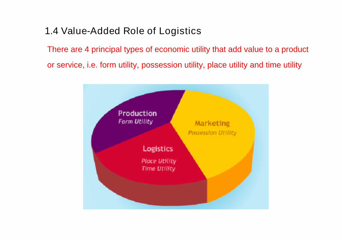
1.4 Value-Added Role of Logistics
There are 4 principal types of economic utility that add value to a product
or service, i.e. form utility, possession utility, place utility and time utility

1.4 Value-Added Role of Logistics
Remember the What, Where, When and Why of the economic utilities
What – Form Utility
Refers to the value added to goods through a manufacturing , production or assembly process.
For example, breaking bulk and product mixing changes a product’s form by changing its
shipment size packaging characteristics
Where – Place Utility
Logistics extends the physical boundaries of the market area, thus adding economic value to
the goods. This addition is known as place utility
When – Time Utility
Goods and services must be available when customers demand them. By having goods and
services available when it is needed creates time utility
Why – Possession Utility
Possession Utility is primarily created by the marketing activities related to the promotion of
goods and services. It increases the desire in a customer to possess a good or to benefit from
a service

Topic 2 – Strategic Supply Chain and Inventory Positioning
Understand the key concepts in supply chain inventory modelling
and its components
- understand the Economic Order Quantity (EOQ)
- know how to determine the Reorder Point (ROP)
- explain the use of the Newsboy Model in inventory replenishment
- understand Pipeline Inventory and its components

2.1 Economic Order Quantity
EOQ is an accounting formula that determines the point at which
the combination of order costs and inventory carrying costs are
the least. The result is the most cost effective quantity to order.
Assumptions used for Economic Order Quantity:
- Demand occurs at a known and reasonably constant rate
- The item has a sufficiently long shelf life
- The item is monitored under a continuous review system
- All the cost parameters remain constant forever (over an infinite time horizon
- A complete order is received in one batch

2.1 Economic Order Quantity
Cost Equation for the Economic Order Quantity (EOQ) Model:
Q* =
where Q* = Optimal order sizeCh = Annual holding cost per unitD = Annual usage in units
Co = Order cost
h
o
C
2DC

2.1 Economic Order Quantity
A graphical representation

2.1 Economic Order Quantity
Sensitivity

1) Economic Order Quantity (EOQ)
Q* =
where Q* = Optimal order size Ch = Annual holding cost per unitD = Annual usage in units Co = Order cost
2) Total Annual Inventory Costs = Total Annual Holding Costs + Total Annual OrderingCosts + Total Annual Procurement Costs
or TC(Q) = (Q/2)Ch + (D/Q)Co + DC
With Safety Stock, the Total Annual Inventory Costs changes to:
TC(Q) =(Q/2)Ch + (D/Q)Co + DC + ChSS
With ChSS being the Safety Stock Holding Costs.
h
o
C
2DC
2.1 Economic Order Quantity
Worked Example

3) Cycle Time (T)
• The cycle time, T, represents the time that elapses between the placement of orders.• Note, if the cycle time is greater than the shelf life, items will go bad, and the modelmust be modified.
T = Q/D
4) Number of Orders per Year (N)
• To find the number of orders per years take the reciprocal of the cycle time
N = D/Q
2.1 Economic Order Quantity
Worked Example

ALLEN APPLIANCE COMPANY (AAC)AAC wholesales small appliances.AAC currently orders 600 units of the Citron brand juicer each time inventorydrops to 205 units.Management wishes to determine an optimal ordering policy for the Citronbrand juicer
Available Data• Co = $12 ($8 for placing an order) + (20 min. to check)($12 per hr)• Ch = $1.40 [HC = (14%)($10)]• C = $10.• H = 14% (10% ann. interest rate) + (4% miscellaneous)• D = demand information of the last 10 weeks was collected:• The constant demand rate seems to be a good assumption.• Annual demand = (120/week) x (52weeks) = 6240 juicers.
Calculate the EOQ and Total Variable Cost.
2.1 Economic Order Quantity
Worked Example

Solution:
EOQ and Total Variable Cost:
Current ordering policy calls for Q = 600 juicers.
TV( 600) = (600/ 2)($1.40) + (6240 / 600)($12) = $544.80
The EOQ policy calls for orders of sizeQ* = = 327.065 = 327TV(327) = (327 / 2)($1.40) + (6240 / 327) ( $12) = $457.89
Under the current ordering policy AAC holds 13 units safety stock.AAC is open 5 day a week.– The average daily demand = 120/week)/5 = 24 juicers.– Lead time is 8 days. Lead time demand is (8)(24) = 192 juicers.– Reorder point without Safety stock = LD = 192.– Current policy: R = 205.– Safety stock = 205 – 192 = 13.
For safety stock of 13 juicers the total cost is
TC(327) = 457.89 + 6240($10) + (13)($1.40) = $62,876.09

Sensitivity of the EOQ Results:
Changing the order size– Suppose juicers must be ordered in increments of 100 (order 300 or 400)
– AAC will order Q = 300 juicers in each order.
– There will be a total variable cost increase of $1.71.
– This is less than 0.5% increase in variable costs.
Changes in input parameters– Suppose there is a 20% increase in demand. D=7500 juicers.
– The new optimal order quantity is Q* = 359.
– The new variable total cost = TV(359) = $502
– If AAC still orders Q = 327, its total variable costs becomes $504
2.1 Economic Order Quantity
Worked Example

Cycle Time
For an order size of 327 juicers we have:T = (327/ 6240) = 0.0524 year.
= 0.0524(52)(5) = 14 days.
This is useful information because:– Shelf life may be a problem.– Coordinating orders with other items might be desirable.
2.1 Economic Order Quantity
Worked Example

2.2 Determining the Reorder Point (ROP)
The following scenarios will be modelled:
Continuous Review – Constant Demand and constant Lead Time
Continuous Review – Variable Demand and constant Lead Time
Fixed Period Review

2.2 Determining the Reorder Point (ROP)
Continuous Review – Constant Demand and constant Lead Time
In reality lead time (LT) always exists, and must be accounted for when deciding at which point in time
to place an order
The reorder point, ROP, is the inventory position when placing an order
The formula to calculate the Reorder point when there is a Constant daily demand (D) and lead-time
(LT) is:
ROP = LT x D
Note: LT and D must be expressed in the same time unit (e.g. per month)

2.2 Determining the Reorder Point (ROP)
Continuous Review – Variable Demand and constant Lead Time
The formula to calculate the Reorder point when there is a Variable daily demand with mean đ and
standard deviation d and lead-time (LT) is:
ROP = đ x LT + z x d x
Note: z represents the service level. It is assumed that the variability in Lead Time follows aNormal Distribution.
The second term on the right represents the Safety Stock. Safety Stock acts as a buffer tohandle higher than average lead time demand and longer than expected lead times.
LΤ

2.2 Determining the Reorder Point (ROP)
Fixed Period Review
Definition of Order up-to-level point (Imax)
Imax = Expected demand during (OI + LT) + safety stock
i.e. Imax = đ x (OI + LT) + z x d x
The Order Quantity is simply the difference between Imax and the quantity on handduring the review
i.e. Order Quantity = Imax – Quantity on Hand
LΤΟΙ

Reorder Point (ROP) Worked Example:
1) Continuous Review (Constant Demand, Constant Lead Time)
Reorder Point R = D x LT
2) Continuous Review (Variable Demand, Constant Lead Time)
Reorder Point R = đ x LT + z x d x
3) Periodic Review (Order up to level or Imax)
Imax is defined as expected demand during order interval (OI) , lead time (LT) and safetystock
i.e. Imax = đ x (OI + LT) + z x d x
Order Quantity = Imax – Quantity on Hand
LΤΟΙ
LΤ

Reorder Point (ROP) Worked Example:
1) Continuous Review (Constant Demand, Constant Lead Time)
A Carpet manufacturer has the following:Daily usage D = 30 yards/dayLead Time LT = 10 days
Reorder Point R = D x LT
= 30 x 10 = 300 yards
2) Continuous Review (Variable Demand, Constant Lead Time)
Additionally, the following is known:
Mean of daily usage đ = 30 yards/dayVariance in demand d = 5 yards/dayService Level of reordering, z = 95% (corresponding to normal variate of 1.65)
Reorder Point R = đ x LT + z x d x
= 30 x 10 + 1.65 x 5 x 10 = 326.1 yards
LΤ

Reorder Point (ROP) Worked Example:
3) Periodic Review (Order up to level or Imax)
Using the following information:
Lead Time LT = 10 daysMean of daily usage đ = 30 yards/dayVariance in demand d = 5 yards/dayService Level of reordering, z = 95%Fixed time between orders OI = 60 days
First compute Imax (defined as expected demand during order interval (OI) , lead time (LT) andsafety stock)
i.e. Imax = đ x (OI + LT) + z x d x
= 30 x (60 + 10) + 1.65 x 5 x (60+10) = 2169 yards
Based on that value of Imax, and at the point of placing the order, the quantity to beordered will be the difference of Imax and the quantity on hand i.e.If Quantity on hand = 450 units,
Order Quantity = Imax – Quantity on Hand
= 2169 – 450 = 1719 yards
LΤΟΙ

2.3 Newsboy Model
The Newsboy Model mimics a person who buys newspapers at
the beginning of the day, sells a random amount and discards any
leftovers.
Here the 2 main issues are:
- Single Replenishment
- The need to determine the appropriate order quantity in the face of uncertain
demand

2.3 Newsboy Model
Insights to the Newsboy Model
• In an environment of uncertain demand, the appropriate production/order
quantity depends on both the distribution of demand and the relative costs of
overproducing versus underproducing.
• In general, increasing the variability (i.e. standard deviation) of demand will
increase the production/order quantity and will therefore increase the likelihood
that the actual demand is far from what is produced/ordered. This implies that
mean and variance of total cost will increase with variability of demand.

2.3 Newsboy Model
G(Q*) – The probability function of the optimum quantity Q*
Co - The unit overage cost is the amount lost per excess set
Cs - The unit shortage cost is the lost profit from a sale
so
s
CC
CQG )( *

Newsboy Model Worked Example:
Consider the following:
A manufacturer of Christmas lights faces a problem each year. Demand issomewhat unpredictable and occurs in such a short burst just prior to Christmasthat if the inventory is not on the shelves, the demand will be lost.
Therefore the decision of how many sets of lights to produce must be made priorto the holiday season. Additionally, the cost of collecting unsold inventory andholding it until next year is too high to make year-to-year storage an attractiveoption. Instead, any unsold sets of lights are sold after Christmas at a steepdiscount.
Suppose that a set of lights costs $1 to make and distribute and is selling for $2.Any sets not sold by Christmas will be discounted to $0.50. Suppose further thatdemand has been forecast to be 10,000 units with a standard deviation of 1,000units and that the normal distribution is a reasonable representation of demand.
How many sets should the manufacturer produce?

Newsboy Model Worked Example:
Preliminary Analysis:
A set of lights costs $1 to make and distribute and is selling for $2.Any sets not sold by Christmas will be discounted to $0.50.
In terms of the above modeling notation, this means that the unit overage cost is theamount lost per excess set or Co = $(1 - 0.50) = $0.50.The unit shortage cost is the lost profit from a sale or Cs = $(2 - 1) = $1.00
The firm could choose to produce 10,000 sets of lights. But, the symmetry (i.e., bellshape) of the normal distribution implies that it is equally likely for demand to be aboveor below 10,000 units.
If demand is below 10,000 units, the firm will lose Co = $0.5 per unit of overproduction.
If demand is above 10,000 units, the firm will lose Cs = $1 per unit of underproduction.
Clearly, shortages are worse than overages.
This suggests that perhaps the firm should produce more than 10,000 units. But, howmuch more?

Newsboy Model Worked Example:
Original Selling Price, OP = $2.00Cost of Production, C = $1.00Discounted Selling Price, DP = $0.50
Assuming the firm could choose to produce 10,000 sets of lights,
The unit overage cost is the amount lost per excess set or Co = $(1.00 - 0.50) = $0.50This means that if demand is below 10,000 units, the firm will lose $0.5 per unit ofoverproduction
The unit shortage cost is the lost profit from a sale or Cs = $(2.00 – 1.00) = $1.00This implies that if demand is above 10,000 units, the firm will lose $1.00 per unit ofunderproduction. Clearly, shortages are worse than overages
Solving for the Probability function, we have:
67.05.01
1
)( *
so
s
CC
CQG

67.05.01
1
000,1
000,10)(
**
QQG
440,10*
44.0000,1
000,10*
67.0)44.0(
Qor
Q
G
Answer: (cont’d)
As its demand is normally distributed,
Where Φ represents the cumulative distribution function of the standard normaldistribution.From a standard normal table, we find that Φ(0.44) = 0.67.Hence, we have:
Note: The Newsboy analysis is only applicable when the goods are time-perishable i.e.
OP > C > DP

Newsboy Model Worked Example:
In which of the following situations, can the Newsboy Model be used?
Scenario 1:Croissants are sold at $1.60 each.Cost of production is $1.20 eachUnsold units are discounted to $0.80 each
Scenario 2:Newspapers are sold at $0.80 each.Cost of production is $0.40 eachUnsold units are discarded i.e. $0 value
Scenario 3:Cookies are sold at $2.80 per packet.Cost of production is $1.20Unsold units are discounted to $2.20

2.4 Pipeline Inventory
The formula below describes the formula to calculate the average
demand during the lead time.
ĎL = đ x LT
Where ĎL is the average demand during the lead time
Example:
đ = 20 units per week
LT = 3 weeks
ĎL = 20 x 3 = 60 units in the pipeline

Topic 3 – Supply Chain Network Design
Appreciate the importance of supply chain network design and its
impact on managing demand
- learn how to cope with Demand Uncertainty
- learn the different types of inventory management:
Centralisation vs Decentralisation
- understand the use of Risk Pooling

3.1 Coping with Demand Uncertainty
The effect of Demand Uncertainty
Most companies treat the world as if it were predictable:
1. Production and inventory planning are based on forecasts of
demand made far in advance of the selling season
2. Companies are aware of demand uncertainty when they create a
forecast, but they design their planning process as if the forecast
truly represents reality

3.1 Coping with Demand Uncertainty
Unfortunately for these companies, there are three principles that
hold true for all forecasting techniques.
Principle 1 :
Forecasting is always wrong
Principle 2 :
The longer the forecast horizon, the worse the forecast
Principle 3 :
Aggregate forecasts are more accurate
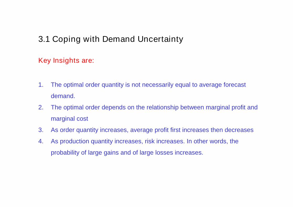
3.1 Coping with Demand Uncertainty
Key Insights are:
1. The optimal order quantity is not necessarily equal to average forecast
demand.
2. The optimal order depends on the relationship between marginal profit and
marginal cost
3. As order quantity increases, average profit first increases then decreases
4. As production quantity increases, risk increases. In other words, the
probability of large gains and of large losses increases.

3.2 Inventory Centralisation/Decentralisation
A Centralised Distribution System is an inventory model that has a single
warehouse serving all customers

3.2 Inventory Centralisation/Decentralisation
A Decentralised Distribution System is an inventory model that has a several
warehouse serving customers with different needs (e.g.
location/product/market)

3.2 Inventory Centralisation/Decentralisation
Whether to centralise or decentralise, depends on the following factors:
Safety Stock
Generally the amount of safety stock decreases when a firm moves from a decentralised to a
centralised system
Service Level
When both centralised and decentralised systems contain the same level of safety stock, the service
level provided by the centralised system is higher
Overhead Costs
These costs are typically higher in a decentralised system because these system enjoys fewer
economies of scale
Customer Lead Time
In decentralised distribution systems, the response time to retailers is shorter because the warehouses
are located much closer to the retailers
Transportation Costs
The net impact of this point is unclear due to the fact that the cost of the outbound deliveries to
retailers decreases for decentralised systems, but at the same time, the costs of delivering the
products to said warehouses increase.

3.2 Inventory Centralisation/Decentralisation
Inventory Management: Best Practices
After a company has decided on which distribution system to adopt, it will need tocontinually reevaluate its inventory levels due to changing demands
Some of the best practices used by most companies include:
• Periodic inventory reviews
• Tight management of usage rates, lead times and safety stock
• ABC approach
• Reduced safety stock levels
• Shift more inventory or inventory ownership, to suppliers
• Quantitative approaches

3.2 Inventory Centralisation/Decentralisation
Changes in Inventory Turnover
With recent developments in information and communication technologies, thetrend in most companies is to increase inventory turnover
This allows companies to increase service levels while keeping inventory costs low
Inventory turnover ratio = annual sales / average inventory level
The following is an indication of Inventory Turnover Ratios used by major players in theindustry:

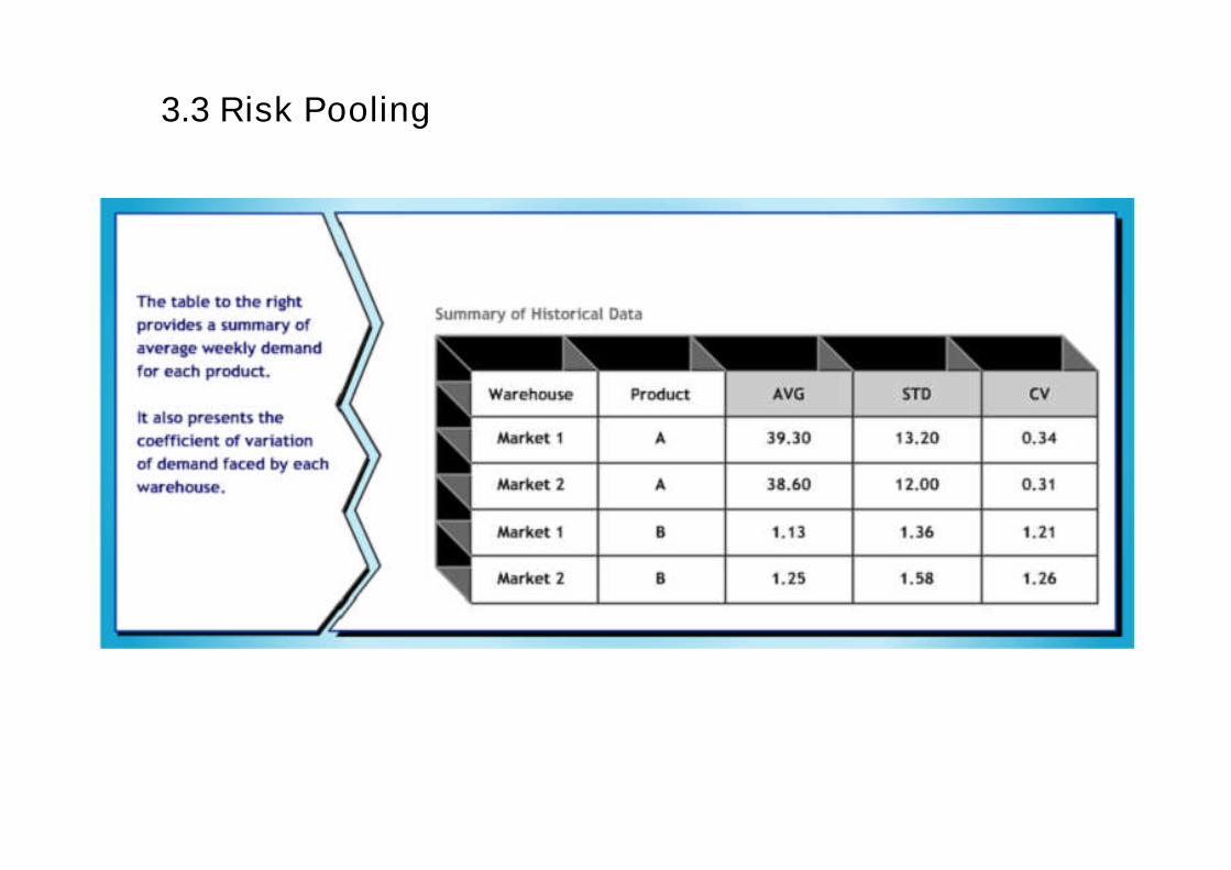
3.3 Risk Pooling
Understanding the concept of Risk Pooling
Risk Pooling is an important concept in supply chain management
• It suggests that demand variability is reduced if one aggregates demand across
locations
• This means that generally, high demand from one customer will be offset by low
demand from another
• This reduction in variability allows a decrease in safety stock and therefore
reduces average inventory

3.3 Risk Pooling
Consider the 2 different systems shown below:

3.3 Risk Pooling
Consider the 2 different systems shown below:
Scenario 1
The primary advantage of usingthis system is that each of thewarehouses are located close toa particular subset of customers,decreasing delivery time

3.3 Risk Pooling
Consider the 2 different systems shown below:
Scenario 2
The advantages of this systemover system 1 are as follows:• With the same inventory level,system 2 can achieve a muchhigher service level.
• With a lower inventory level,system 2 can achieve the sameservice level.

3.3 Risk Pooling
The reason why system 2 is more efficient is because it fulfills random demand
• A higher than average demand at one retailer will usually be offset by a lower
than average demand from another retailer.
• As the number of retailers served by a warehouse increases, the likelihood of
offsetting occurrence will also increase
• By centralising inventories, a company can ensure a higher service level and
lower the possibility of a stockout.

3.3 Risk Pooling

3.3 Risk Pooling

3.3 Risk Pooling
3.3 Risk Pooling

3.3 Risk Pooling

3.3 Risk Pooling
In conclusion, the 3 critical points of Risk Pooling are:
• Centralising inventory reduces both safety stock and average inventory in the
system for the same service level. It also allows the reallocation of inventory
from one market segment to another when the situation requires it.
• The higher the coefficient of variation, the greater the benefit obtained from
risk pooling. This is because the need for keeping a higher level of safety stock
is reduced when there is risk pooling.
• The benefits of risk pooling depend on the behaviour of demand from one
market relative to another. Demand in two markets is positively correlated if it
is very likely that an increase in demand in one market related in an increase
in demand in the other. In these cases, the benefit of risk poling decreases
when the correlation between two markets become increasingly positive.

Topic 4 – Best Practices in Supply Chain Management
Understand the emerging principles of supply chain management
using postponement
- justify the use of Express Logistics
- explain the various types of Postponement methods
- using Cross Docking to minimise storage costs

4.1 The Value of Express Logistics

4.1 The Value of Express Logistics

4.1 The Value of Express Logistics

4.1 The Value of Express Logistics

4.2 The Value of Postponement
In this section, postponement refers specifically to form postponement and
looks into:
• Design product and manufacturing processes so that decisions about specific
products can be delayed as late as possible
• This process is also known as Delayed Point Differentiation (DPD) or Late
Point Differentiation (LPD)
• The primary benefit is to reduce demand uncertainty thereby increasing
service level delay and reducing inventory costs

4.2 The Value of Postponement
Compare the 2 supply chain processes below to see how postponement changes the
process of delivering the end product to consumers.

4.2 The Value of Postponement

4.2 The Value of Postponement

4.2 The Value of Postponement

4.3 The Value of Cross-Docking
In this section, we will examine the Cross-Docking process in the following
ways:
• Understand the flow of Cross-Docking and how products are delivered from
the manufacturer to the retailer
• Examine the challenges associates with using Cross-Docking
• Explore the different options in which Cross-Docking can be applied

4.3 The Value of Cross-Docking
Cross-Docking is a process where products are moved directly from receiving to the shipping dock with no or very short interim
storage.
The main users of Cross-Docking are mass merchandisers, grocery companies, LTL trucking companies, air cargo carriers….etc
The products usually associated with Cross-Docking include seasonal items, promotional goods, store-specific pallets or high
volume items.

4.3 The Value of Cross-Docking

4.3 The Value of Cross-Docking

4.3 The Value of Cross-Docking

4.3 The Value of Cross-Docking
Options available to implementing Cross-Docking
Option 1 – Basic Cross-Docking
4.3 The Value of Cross-Docking
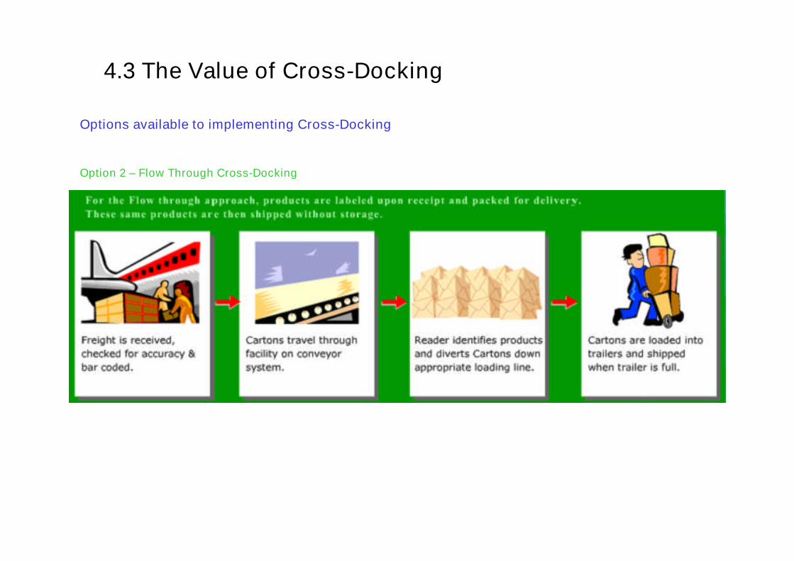
Options available to implementing Cross-Docking
Option 2 – Flow Through Cross-Docking

4.3 The Value of Cross-Docking
Examples:
1. The NUMMI plant in California uses cross-docks in Chicago and Memphis
to collect, consolidate and sort freight from multiple vendors into
containers that are shipped via rail to the plant
2. Suppliers send parts in bulk to General Motor’s cross-dock in Memphis.
Parts are sorted for delivery to 15 different production facilities in the
Midwest.

Topic 5 – Resource Planning and Optimisation
Evaluate the different modes of matching demand with supply and
their trade-offs
- understand the Theory of Constraints (TOC)
- explain the logic of Materials Requirement Planning (MRP)
- understand Enterprise Resource Planning (ERP) and its components

5.1 Theory of Constraints

5.1 Theory of Constraints

5.1 Theory of Constraints
Constraints fall into three categories

5.1 Theory of Constraints
Constraints fall into three categories

5.1 Theory of Constraints
Constraints fall into three categories

5.1 Theory of Constraints

5.1 Theory of Constraints

5.1 Theory of Constraints

5.1 Theory of Constraints

5.1 Theory of Constraints

5.1 Theory of Constraints

5.1 Theory of Constraints

5.1 Theory of Constraints

5.1 Theory of Constraints

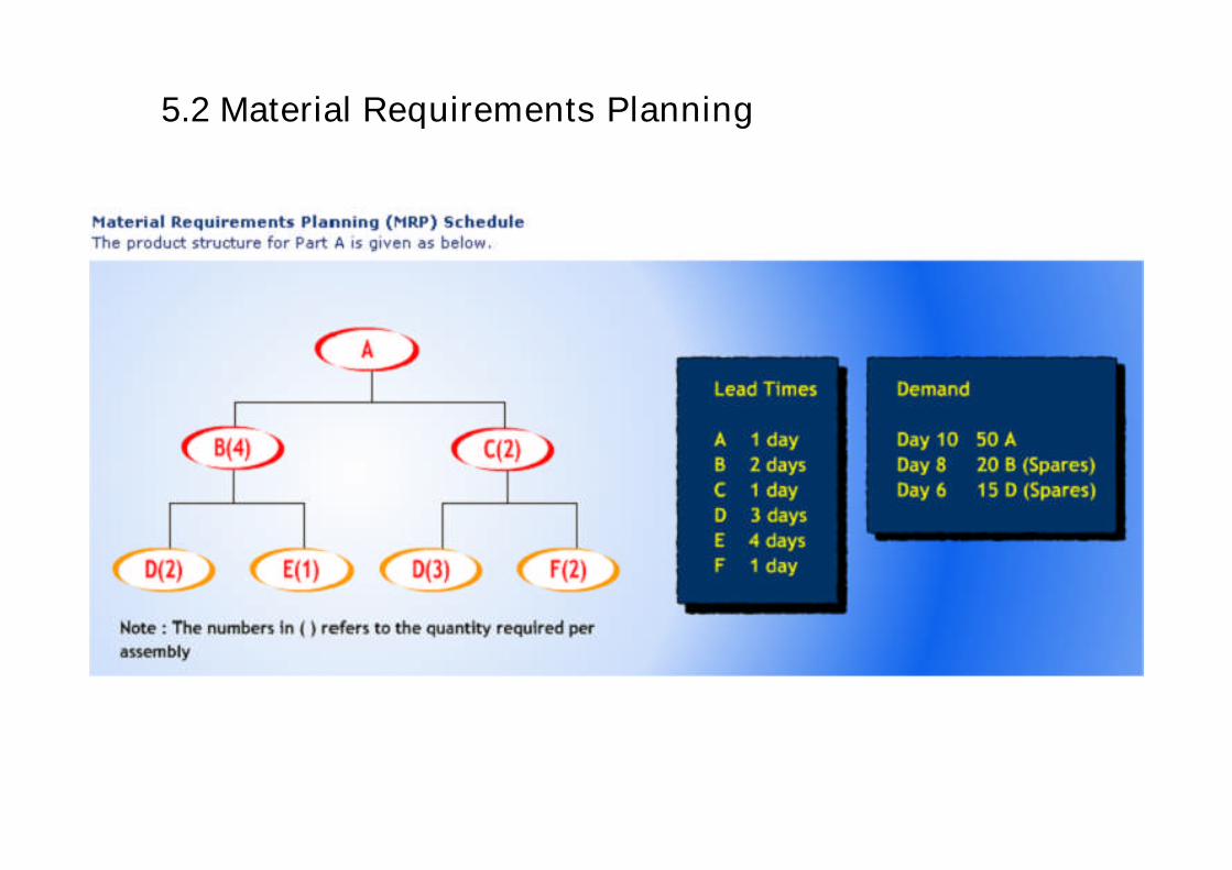
5.2 Material Requirements Planning

5.2 Material Requirements Planning

5.2 Material Requirements Planning

5.2 Material Requirements Planning

5.2 Material Requirements Planning
5.2 Material Requirements Planning

Steps in creating the Materials Requirement Plan
1) Create a timeline based on the required deadline
2) First 2 rows consist of the final product – Required row, followed by Order placement
3) Create subsequent rows based on the the order the part appears in the Bill ofMaterials (BOM)
4) Populate the table with the Required quantity of the finished assembly
5) Note the lead time, and populate the Order Placement of the finished assembly,remembering to offset by the lead time
6) From the BOM, trace the relationship with the next level, and populate the Requiredquantity from the Order quantity of the parent part (remembering to factor in theproportions)
7) Note the lead time, and populate the Order Placement of the part, remembering tooffset by the lead time
8) Repeat this until you reach individual parts which do not have any sub-parts
5.2 Material Requirements Planning

5.2 Material Requirements Planning

B (2)
E (4)
C (2) D (3)
ALead Times DemandA – 1 day Day 6 – 100 units of AB – 3 daysC – 2 daysD – 1 dayE – 2 days
Another MRP example
Based on the information, work out the Materials Requirement Plan
5.2 Material Requirements Planning

MRP example - solution
800OrderPlacement
800RequiredE
300OrderPlacement
300RequiredD
200OrderPlacement
200RequiredC
200OrderPlacement
200RequiredB
100OrderPlacement
100RequiredA
654321Day
5.2 Material Requirements Planning

5.2 Material Requirements Planning
Time Fences:
• Frozen – No schedule changes are allowed within this window
• Moderately Firm – Specific changes are allowed within product groups as
long as parts are available
• Flexible – Signification variation is allowed as long as overall capacity
requirements remain the same levels

5.2 Material Requirements Planning
Time Fences:
The graph below illustrates the relationship between demand and time fences.

5.3 Enterprise Requirements Planning
Definition:
• An ERP or Enterprise Resource Planning
system integrates information and business
processes to enable information entered once to
be shared throughout the organisation.
• ERP (Enterprise Resource Planning) is an
industry term for the broad set of activities
supported by multi-module application software
that helps an organisation to manage the
important part of its business.

5.3 Enterprise Requirements Planning

5.3 Enterprise Requirements Planning
Components of ERP
The diagram below illustrates the anatomy of an ERP application.

5.3 Enterprise Requirements Planning
Components of ERP
The diagram below illustrates the anatomy of an ERP application.
5.3 Enterprise Requirements Planning
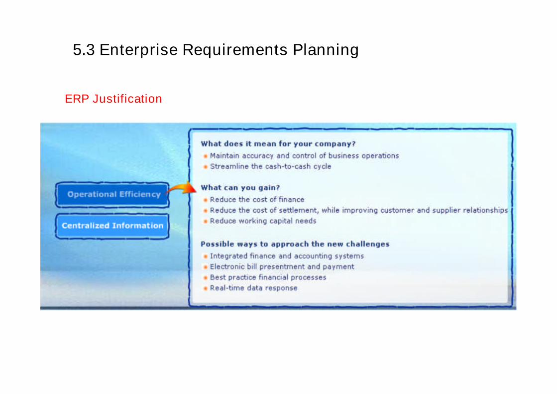
ERP Justification

5.3 Enterprise Requirements Planning
ERP Justification

5.3 Enterprise Requirements Planning

5.3 Enterprise Requirements Planning

5.3 Enterprise Requirements Planning

5.3 Enterprise Requirements Planning

5.3 Enterprise Requirements Planning
Topic 6 – Forecasting and JIT
Understand the various forecasting methods to increase accuracy
and the JIT techniques to reduce wastages
- explain the various types of forecasting and aggregate planning
- understand Just-in-Time (JIT) production system

6.1 Forecasting and Aggregate Planning

6.1 Forecasting and Aggregate Planning

Forecasting Methods are classified according to the following
four types:
1. Qualitative
Qualitative Forecasting methods are primarily subjective and rely on human judgment. They are
most appropriate when there is little historical data available or when experts have market
intelligence that is critical in making the forecast. Such methods may be necessary to forecast
demand several years into the future in a new industry.
2. Time Series
Time Series Forecasting methods use historical demand to make a forecast. They are based on the
assumption that past demand history is a indicator of future demand. These methods are most
appropriate when the basic demand pattern does not vary significantly from one year to the next.
These are the simplest methods to implement and can serve as a good starting point for a demand
forecast.
6.1 Forecasting and Aggregate Planning

Forecasting Methods (cont’d)
3. Causal
Causal Forecasting methods assume that the demand forecast is highly correlated with certain
factors in the environment (e.g. the state of the economy, interest rates etc). Causal forecasting
methods find this correlation between demand and environmental factors and use estimates of
what environmental factors will be to forecast future demand. For example, product pricing is
strongly correlated with demand. Companies can thus use causal methods to determine the
impact of price promotions on demand.
4. Simulation
Simulation forecasting methods imitate the customer choices that give rise to demand to arrive at a
forecast. Using simulation, a firm can combine time series and causal methods to answer such
questions as: what will the impact of a price promotion be? What will the impact be of a competitor
opening a store nearby? Airlines simulate customer buying behaviour to forecast demand for
higher fare seats when there are no seats available at the lower fares.
6.1 Forecasting and Aggregate Planning

6.1 Forecasting and Aggregate Planning

6.1 Forecasting and Aggregate Planning

6.1 Forecasting and Aggregate Planning

6.1 Forecasting and Aggregate Planning

6.1 Forecasting and Aggregate Planning

6.1 Forecasting and Aggregate Planning

6.1 Forecasting and Aggregate Planning

6.1 Forecasting and Aggregate Planning

6.1 Forecasting and Aggregate Planning

Define Objective Function
Denote the demand in Period t by Dt. The objective function is tominimize the total cost (equivalent to maximizing total profit as alldemand is to be satisfied) incurred during the planning horizon. The costincurred has the following components:
• Regular time labor cost• Overtime labor cost• Cost of hiring and layoffs• Cost of holding inventory• Cost of stocking out• Cost of subcontracting• Material cost
6.1 Forecasting and Aggregate Planning

1. Regular time labor cost.
Workers are paid a regular time wage of $640 ($4/hour x eight hours/dayx twenty days/month) per month. Because Wt is the number of workersin Period t, the regular time labor cost over the planning horizon is givenby the following:
Regular time labor cost =
6.1 Forecasting and Aggregate Planning
Define Objective Function
2. Overtime labor cost.
Overtime labor cost is $6 per hour and Ot represents the number ofovertime hours worked in Period t, the overtime cost over theplanning horizon is given as follows:
Overtime labor cost =

3. Cost of hiring and layoffs.
The cost of hiring a worker is $300 and the cost of laying off a worker is$500. Ht and Lt represent the number hired and the number laid offrespectively in Period t. Thus the cost of hiring and layoff is given by thefollowing:
Cost of hiring and layoffs =
4. Cost of inventory and stockout.
The cost of carrying inventory is $2 per unit per month and the cost ofstocking out is $5 per unit per month. It and St represent the units ininventory and the units stocked out, respectively, in Period t. Thus, thecost of holding inventory and stocking out is given as follows:
Cost of holding inventory and stocking out =
6.1 Forecasting and Aggregate Planning
Define Objective Function

5. Cost of materials and subcontracting.
The material cost is $10 per unit and the subcontracting cost is$30/unit. Pt represents the quantity produced and Ct represents thequantity subcontracted in Period t. Thus, the material andsubcontracting cost is given by the following:
Cost of materials and subcontracting =
6.1 Forecasting and Aggregate Planning
Define Objective Function

6.1 Forecasting and Aggregate Planning
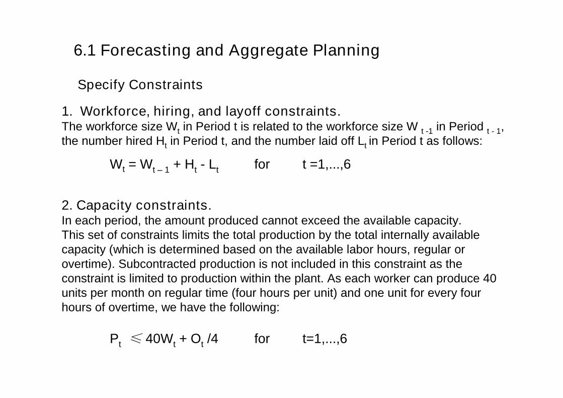
Specify Constraints
1. Workforce, hiring, and layoff constraints.The workforce size Wt in Period t is related to the workforce size W t -1 in Period t - 1,the number hired Ht in Period t, and the number laid off Lt in Period t as follows:
Wt = Wt – 1 + Ht - Lt for t =1,...,6
2. Capacity constraints.In each period, the amount produced cannot exceed the available capacity.This set of constraints limits the total production by the total internally availablecapacity (which is determined based on the available labor hours, regular orovertime). Subcontracted production is not included in this constraint as theconstraint is limited to production within the plant. As each worker can produce 40units per month on regular time (four hours per unit) and one unit for every fourhours of overtime, we have the following:
Pt ≤ 40Wt + Ot /4 for t=1,...,6
6.1 Forecasting and Aggregate Planning

3. Inventory balance constraints.The third set of constraints balances inventory at the end of each period. Netdemand for Period t is obtained as the sum of the current demand Dt and theprevious backlog S t -1. This demand is either filled from current production(inhouse production Pt or subcontracted production Ct) and previous inventory It-1(in which case some inventory It may be left over) or part of it is backlogged St.This relationship is captured by the following equation:
I t- 1 + Pt+ Ct= Dt +St-1 + It - St for t = I, . . , 6
4. Overtime limit constraints.The fourth set of constraints requires that no employee work more than ten hoursof overtime each month. This requirement limits the total amount of overtimehours available as follows:
Ot ≤ 10Wt for t =1,…6
Specify Constraints
6.1 Forecasting and Aggregate Planning

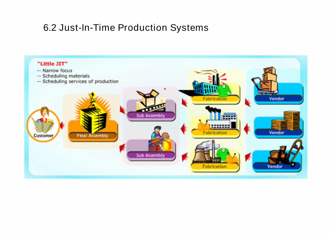
6.2 Just-In-Time Production Systems
Definition of Just-In-Time (JIT) Production System

Definition of Just-In-Time (JIT) Production System
6.2 Just-In-Time Production Systems

Definition of Just-In-Time (JIT) Production System
6.2 Just-In-Time Production Systems

Definition of Just-In-Time (JIT) Production System
6.2 Just-In-Time Production Systems

Definition of Just-In-Time (JIT) Production System
6.2 Just-In-Time Production Systems

6.2 Just-In-Time Production Systems
6.2 Just-In-Time Production Systems

• Waste from overproduction
• Waste of waiting time
• Transportation waste
• Inventory waste
• Processing waste
• Waste due to movement
• Waste from product defects
Types of waste in operation
6.2 Just-In-Time Production Systems

Ways in Minimising Waste
6.2 Just-In-Time Production Systems

Ways in Minimising Waste
Inventory Hides Problems
6.2 Just-In-Time Production Systems

Ways in Minimising Waste
Kanban System
Kanban
A Kanban or signboard is attached to specific parts in the production line to signify the delivery of a given quantity. When theparts have all been used, the same sign is returned to its origin where it becomes an order for more.
Kanban Signal
A method of signaling suppliers or upstream operations when it is time to replenish limited stocks of components orsubassemblies in a just-in-time system. Originally a card system used in Japan, kanban signals now include emptycontainers, empty spaces and even electronic messages.
6.2 Just-In-Time Production Systems

Ways in Minimising Waste
Focused Factory Networks
6.2 Just-In-Time Production Systems

Ways in Minimising Waste
Group Technology
6.2 Just-In-Time Production Systems

Ways in Minimising Waste
Quality at Source
6.2 Just-In-Time Production Systems

Ways in Minimising Waste
Uniform Plant Loading
6.2 Just-In-Time Production Systems

Methodology
6.2 Just-In-Time Production Systems

Methodology
6.2 Just-In-Time Production Systems

Methodology
6.2 Just-In-Time Production Systems

Methodology
6.2 Just-In-Time Production Systems

Methodology
6.2 Just-In-Time Production Systems

Methodology
6.2 Just-In-Time Production Systems

Methodology
6.2 Just-In-Time Production Systems

Applying JIT Concepts
6.2 Just-In-Time Production Systems

Reference Text
The Management of Business Logistics:A Supply Chain Perspective
7th Edition
COYLE . BARDI . LANGLEY
ISBN 0-324-00751-5