mit opencourseware 6.013/esd.013j … · markus zahn, erich ippen, and david staelin,...

MIT OpenCourseWare http://ocw.mit.edu 6.013/ESD.013J Electromagnetics and Applications, Fall 2005 Please use the following citation format:

Markus Zahn, Erich Ippen, and David Staelin, 6.013/ESD.013J Electromagnetics and Applications, Fall 2005. (Massachusetts Institute of Technology: MIT OpenCourseWare). http://ocw.mit.edu (accessed MM DD, YYYY). License: Creative Commons Attribution-Noncommercial-Share Alike.

Note: Please use the actual date you accessed this material in your citation. For more information about citing these materials or our Terms of Use, visit: http://ocw.mit.edu/terms

http://ocw.mit.edu

http://ocw.mit.edu

http://ocw.mit.edu/terms

6.013, Electromagnetic Fields, Forces, and Motion Prof. Markus Zahn

Lecture 18: Fields and Moving Media November 15,2005

I. Ohm’s Law in Moving Media

Force on moving charge: ( )f q E v B= + ×

Consider force on moving charge in reference frame (denoted as prime (') frame)

moving at charge velocity v . Then f qE′ ′= as in the moving frame the relative velocity is zero.

With v constant, f and f ′ are inertial frames (non-accelerating) so that:

( )f f qE q E v B E E v B′ ′ ′= ⇒ = + + ⇒ = + +

in primed frame: ( )J E E v Bσ σ′ ′= = + ×

If system is charge neutral, as is usual case in MQS systems

( )J J E vσ′= = + ×B

II. Moving Media MQS Problem

6.013, Electromagnetic Fields, Forces, and Motion Lecture 18 Prof. Markus Zahn Page 1 of 20

Moving Contour C

C S

dE ' dl = B n da

dt−∫ ∫i i

− − − ξ⎡ ⎤⎣ ⎦d

v = B hdt

B and n in opposite directions

ξ

− −d

v = B h = B h Vdt

Stationary Contour C’

−∫ ∫i iC ' S'

dE dl = B n da = 0

dt

+ ×E ' = 0 = E v B in moving perfect conductor

( )− + ×y

v v B h = 0

−v = Bh V


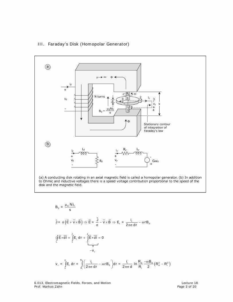
III. Faraday’s Disk (Homopolar Generator)

µ0 f0

N iB =

s

( )σ + × ⇒ − × ⇒ − ωσ πσ

rr 0

iJJ = E v B E = v B E = rB

2 dr

2 4

rL 1 3

E dl E dr E dl 0= +∫ ∫ ∫i i =

− rv

( )−ω⎛ ⎞− ω −⎜ ⎟πσ πσ⎝ ⎠

∫ ∫0

i

R22 20 0r r

r r 0 0i1 R

R Bi iv = E dr = rB dr = ln R R

2 dr 2 d R 2 i


− ωr r f= i R G i

( )µ−

πσ

0

2 20ir 0

Rln NRR = , G = R R

2 d 2s i

Representative Numbers: copper ( )76 x 10 siemen / m , d = 1mmσ ≈

ω π= 3600rpm = 120 rad / s 0 i 0R = 10 cm, R = 1cm, B = 1 tesla

( )−ω− ≈ −2 20

0c 0 i

Bv = R R 1.9 V

2

πσ

≈⎛ ⎞⎜ ⎟⎝ ⎠

50csc

0

i

v 2 di = 3 x10 amp

Rln R

( )π

φ= = =

× × φ∫ ∫ ∫0

i

R2 d

r0 z 0 r R

T = r i J B r dr d dz

0

i

R_

zr 0R

= i B i r dr− ∫

( )_

2 2r 0z0 i

i B= R R

2−

− i

_

zf r= G i i i−


IV. Self-Excited DC Homopolar Generator

f ri = i i≡

( )+ − ω +r f

diL i R G = 0 ; R = R

dtR

r fL = L L+

( ) [ ]− − ωR G t /L0i t = I e

ω >G R Self-Excited


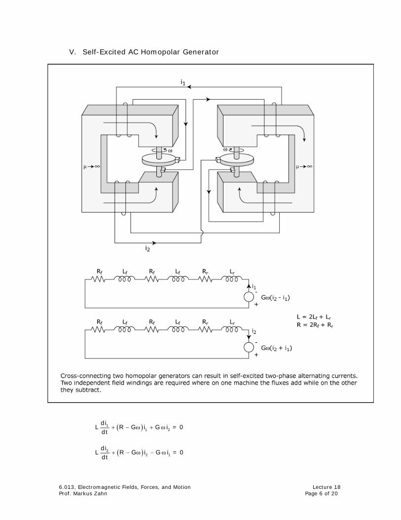
V. Self-Excited AC Homopolar Generator

( )+ − ω + ω11 2

diL R G i G i =

dt0

( )+ − ω − ω22 1

diL R G i G i =

dt0


st st

1 1 2 2i = I e , i = I e ( )+ − ω + ω1 2Ls R G I G I = 0

( )− ω + + − ω1 2G I Ls R G I = 0

( ) ( )+ − ω + ω2 2

Ls R G G = 0

+ − ω ± ωLs R G = jG

( )− ω ω

− ±R G G

s = jL L

( )− ω

±+ − ω

1

2

I G= = j

I Ls R G

Self Excited: G > R ω Oscillation frequency: ( )ω ω0 m= I s = G L


VI. Self-Excited Periodic Motor Speed Reversals

( )− ω ω+ g g m m f

R G i G Idi=

dt L L


ω

−mm f

dJ = G I

dti

ωst stmi = Ie , = We

− ω⎡ ⎤ ⎛ ⎞

+ −⎢ ⎥ ⎜ ⎟⎝ ⎠⎣ ⎦

g g m fR G G I

I s W = 0L L

⎛ ⎞+⎜ ⎟

⎝ ⎠m fG I

I WsJ

= 0

( )− ω⎡ ⎤+ +⎢ ⎥

⎣ ⎦

2

g g m fR G G Is s = 0

L JL

( ) ( )⎡ ⎤− ω − ω⎛ ⎞⎢ ⎥− ± −⎜ ⎟⎢ ⎥⎝ ⎠⎣ ⎦

12 22

g g g g m fR G R G G I

s =2 L 2 L JL

Self-excitation: G R ω >g g

Oscillations if s has an imaginary part:

( ) − ω⎛ ⎞> ⎜ ⎟⎝ ⎠

22

g gm f R GG I

JL 2 L

VII. DC Commutator Machines

Quasi-One Dimensional Description

A. Electrical Equations


C S

dE dl = B nda

dt−∫ ∫i i


1. Field Winding

− + − +σ∫ ∫i f

f fC w

f f

iE dl = v dl = v i R

inding A

Resistance of field winding

Jσ

f fS

= B nda = L iλ ∫ i f

− + − ff f f f

div i R = L

dt

+ff f f

div = L i R

dt f

2. Armature Winding


Reminder: ( )+ ×f = q E v B = qE'

+ ×E' = E v B

Take Stationary Contour through armature winding

− ×E = E' v B

( )− + − ×∫ ∫i iaC

E dl = v E' v B dl

θ⎛ ⎞

− + + ω ω⎜ ⎟σ⎝ ⎠∫ ib _ _

aza r

a

i= v RB i dl ; v = R i

A

( )r rB = i B χ

( )− + + ωa a a rf av

= v i R R B lN

aa

S

did= B da = L

dt dt− −∫ i

( )( )+ + ωaa a a a f f rf av

div = i R L G i Gi = lNR B

dt

B. Mechanical Equations

_ _ _a

z r r w a rw

iF = i J B = i B , f = F A l = i i lB

Aθ θ θ

a r f aT = f R = i lB RN = Gi i

2

f a2

dJ = T = Gidtθ

i

C. Linear Amplifier 1) Open Circuit

⇒f f a f fv = V , i = 0 i = V Rf

ωa fv = G V Rf

2) Resistively Loaded Armature (DC Generator)

− + ωa a L a a fv = i R = i R G V Rf


( )− ω

+f

af a L

G Vi =

R R R

( )ω

+f L

af a L

G V Rv =

R R R

D. DC Motors 1) Shunt Excitation:

a fv = v = vt

f

a

+ ωt f f a av = i R = i R G i ( )− ωf f ai R G = i R

( )− ωft t

f af f a

R GV Vi = , i =

R R R

( )− ω⎛ ⎞⎜ ⎟⎝ ⎠

2

ftf a

f a

R GVT = Gi i = G

R R


2) Series: a fi = i = it

t

( )+ + ωt f ai R R G = v

( )+ + ωt

tf a

vi =

R R G

( )+ + ω

22 t

t 2

f a

vT = Gi = G

R R G


VIII. Self-Excited Machines


mit opencourseware 6.013/esd.013j … · markus zahn, erich ippen, and david staelin,...

Documents