mitigation of wind-induced vibration of stay cables ... . cable-stayed bridges have become the form...

Research, Development, and TechnologyTurner-Fairbank Highway Research Center6300 Georgetown PikeMcLean, VA 22101-2296

Mitigation of Wind-Induced Vibration ofStay Cables: Numerical Simulationsand EvaluationsPUBLICATION NO. FHWA-HRT-14-049 AUGUST 2014

FOREWORD

Cable-stayed bridges have become the form of choice over the past several decades for bridges in the medium-to-long-span range. In some cases, serviceability problems involving large amplitude vibrations of stay cables under certain wind and wind-rain conditions have been observed. This study was conducted in response to State transportation departments’ requests to develop improved design guidance for mitigation of excessive cable vibrations on cable-stayed bridges. The study included finite element modeling of representative individual cables as well as networks of cables to simulate dynamic behavior and evaluate various mitigation details such as dampers and crossties. The results of this study will be made available to the DC-45 Cable-Stayed Bridge Committee for the Post-Tensioning Institute for consideration during their periodic updates of the Guide Specification, Recommendations for Stay Cable Design, Testing, and Installation.(1)

This report will be of interest to bridge engineers, wind engineers, and consultants involved in the design of cable-stayed bridges. It is the first in a series of reports addressing aerodynamic stability of bridge stay cables that will be published in the coming months.

Jorge E. Pagán-Ortiz Director, Office of Infrastructure Research and Development

Notice This document is disseminated under the sponsorship of the U.S. Department of Transportation in the interest of information exchange. The U.S. Government assumes no liability for the use of the information contained in this document. This report does not constitute a standard, specification, or regulation.

The U.S. Government does not endorse products or manufacturers. Trademarks or manufacturers’ names appear in this report only because they are considered essential to the objective of the document.

Quality Assurance Statement The Federal Highway Administration (FHWA) provides high-quality information to serve Government, industry, and the public in a manner that promotes public understanding. Standards and policies are used to ensure and maximize the quality, objectivity, utility, and integrity of its information. FHWA periodically reviews quality issues and adjusts its programs and processes to ensure continuous quality improvement.

TECHNICAL DOCUMENTATION PAGE 1. Report No. FHWA-HRT-14-049

2. Government Accession No.

3. Recipient’s Catalog No.

4. Title and Subtitle Mitigation of Wind-Induced Vibration of Stay Cables: Numerical Simulations and Evaluations

5. Report Date August 2014 6. Performing Organization Code

7. Author(s) Sunwoo Park and Harold R. Bosch

8. Performing Organization Report No.

9. Performing Organization Name and Address Genex Systems, LLC 2 Eaton Street, Suite 603 Hampton, VA 23669

10. Work Unit No. (TRAIS) 11. Contract or Grant No. DTFH61-07-D-00034

12. Sponsoring Agency Name and Address Office of Infrastructure R&D Federal Highway Administration 6300 Georgetown Pike McLean, VA 22101-2296

13. Type of Report and Period Covered Laboratory Report December 2003–December 2008 14. Sponsoring Agency Code HRDI-50

15. Supplementary Notes The Contracting Officer’s Technical Representative (COTR) was Harold R. Bosch, HRDI-50. 16. Abstract Cable-stayed bridges have been recognized as the most efficient and cost effective structural form for medium-to-long-span bridges over the past several decades. With their widespread use, cases of serviceability problems associated with large amplitude vibration of stay cables have been reported. Stay cables are laterally flexible structural members with very low inherent damping and thus are highly susceptible to environmental conditions such as wind and rain/wind combination.

Recognition of these problems has led to the incorporation of different types of mitigation measures on many cable-stayed bridges around the world. These measures include surface modifications, cable crossties, and external dampers. Modifications to cable surfaces have been widely accepted as a means to mitigate rain/wind vibrations. Recent studies have firmly established the formation of a water rivulet along the upper side of the stay and its interaction with wind flow as the main cause of rain/wind vibrations. Appropriate modifications to exterior cable surfaces effectively disrupt the formation of a water rivulet.

The objective of this study is to supplement the existing knowledge base on some of the outstanding issues of stay cable vibrations and to develop technical recommendations that may be incorporated into design guidelines. Specifically, this project focuses on the effectiveness of cable crossties, external dampers, and the combined use of crossties and dampers. Finite element simulations are carried out on the stay cable systems of constructed stay cable bridges under realistic wind forces in order to address these issues. Explicit time-history analysis enabled the performance of stay cable systems with different mitigation strategies to be assessed and compared for their relative advantages and disadvantages. 17. Key Words Cable-stayed bridges, Cables, Vibrations, Wind, Rain, Dampers, Crossties, Hazard mitigation, Simulation

18. Distribution Statement No restrictions. This document is available to the public through the National Technical Information Service, Springfield, VA 22161.

19. Security Classif. (of this report) Unclassified

20. Security Classif. (of this page) Unclassified

21. No. of Pages 115

22. Price

Form DOT F 1700.7 (8-72) Reproduction of completed page authorized

SI* (MODERN METRIC) CONVERSION FACTORS APPROXIMATE CONVERSIONS TO SI UNITS

Symbol When You Know Multiply By To Find Symbol LENGTH

in inches 25.4 millimeters mm ft feet 0.305 meters m yd yards 0.914 meters m mi miles 1.61 kilometers km

AREA in2 square inches 645.2 square millimeters mm2

ft2 square feet 0.093 square meters m2

yd2 square yard 0.836 square meters m2

ac acres 0.405 hectares ha mi2 square miles 2.59 square kilometers km2

VOLUME fl oz fluid ounces 29.57 milliliters mL gal gallons 3.785 liters L ft3 cubic feet 0.028 cubic meters m3

yd3 cubic yards 0.765 cubic meters m3

NOTE: volumes greater than 1000 L shall be shown in m3

MASS oz ounces 28.35 grams glb pounds 0.454 kilograms kgT short tons (2000 lb) 0.907 megagrams (or "metric ton") Mg (or "t")

TEMPERATURE (exact degrees) oF Fahrenheit 5 (F-32)/9 Celsius oC

or (F-32)/1.8 ILLUMINATION

fc foot-candles 10.76 lux lx fl foot-Lamberts 3.426 candela/m2 cd/m2

FORCE and PRESSURE or STRESS lbf poundforce 4.45 newtons N lbf/in2 poundforce per square inch 6.89 kilopascals kPa

APPROXIMATE CONVERSIONS FROM SI UNITS Symbol When You Know Multiply By To Find Symbol

LENGTHmm millimeters 0.039 inches in m meters 3.28 feet ft m meters 1.09 yards yd km kilometers 0.621 miles mi

AREA mm2 square millimeters 0.0016 square inches in2

m2 square meters 10.764 square feet ft2

m2 square meters 1.195 square yards yd2

ha hectares 2.47 acres ac km2 square kilometers 0.386 square miles mi2

VOLUME mL milliliters 0.034 fluid ounces fl oz L liters 0.264 gallons gal m3 cubic meters 35.314 cubic feet ft3

m3 cubic meters 1.307 cubic yards yd3

MASS g grams 0.035 ounces ozkg kilograms 2.202 pounds lbMg (or "t") megagrams (or "metric ton") 1.103 short tons (2000 lb) T

TEMPERATURE (exact degrees) oC Celsius 1.8C+32 Fahrenheit oF

ILLUMINATION lx lux 0.0929 foot-candles fc cd/m2 candela/m2 0.2919 foot-Lamberts fl

FORCE and PRESSURE or STRESS N newtons 0.225 poundforce lbf kPa kilopascals 0.145 poundforce per square inch lbf/in2

*SI is the symbol for th International System of Units. Appropriate rounding should be made to comply with Section 4 of ASTM E380. e(Revised March 2003)

ii

TABLE OF CONTENTS

EXECUTIVE SUMMARY .......................................................................................................... 1

CHAPTER 1: INTRODUCTION ................................................................................................ 3

CHAPTER 2: THEORETICAL BACKGROUND .................................................................... 5 VIBRATION OF TAUT STRINGS ...................................................................................... 5 VIBRATION OF CLASSICAL BEAMS .............................................................................. 6 VIBRATION OF TAUT STRINGS WITH FLEXURAL STIFFNESS ............................ 7 VIBRATION OF TAUT STRINGS WITH FLEXURAL STIFFNESS AND SAG-EXTENSIBILITY ......................................................................................................... 8

CHAPTER 3: PRELIMINARY ANALYSIS OF STAY CABLE VIBRATIONS ................ 11 INTRODUCTION................................................................................................................. 11 NUMERICAL MODELING AND ANALYSIS OF STAY CABLES .............................. 11

Taut String Model ............................................................................................................. 11 Classical Beam .................................................................................................................. 13 Taut String with Flexural Stiffness ................................................................................... 14

TWO-CABLE SYSTEM WITH CROSSTIE ..................................................................... 16 FULL-SCALE STAY CABLE NETWORK ...................................................................... 20

Vibration Mode Shapes..................................................................................................... 20 Mode-Frequency Evolution .............................................................................................. 24 Variations in Crosstie Configuration ................................................................................ 25

CHAPTER 4: FREE-VIBRATION ANALYSIS OF STAY CABLE SYSTEMS WITH CROSSTIES .................................................................................................................... 31

INTRODUCTION................................................................................................................. 31 NATURAL FREQUENCIES AND MODE SHAPES ....................................................... 35 INFLUENCE OF CROSSTIE QUANTITY ....................................................................... 38 INFLUENCE OF CROSSTIE GEOMETRY .................................................................... 47 INFLUENCE OF CROSSTIE DIAMETER ...................................................................... 51 INFLUENCE OF OTHER PARAMETERS ...................................................................... 52 OUT-OF-PLANE BEHAVIOR ........................................................................................... 55

CHAPTER 5: TIME-HISTORY ANALYSIS OF STAY-CABLE SYSTEMS WITH CROSSTIES .................................................................................................................... 57

INTRODUCTION................................................................................................................. 57 WIND LOADS ...................................................................................................................... 57 PERFORMANCE UNDER REFERENCE WIND LOAD ............................................... 59

Displacements ................................................................................................................... 59 Energy Evolution .............................................................................................................. 64

PERFORMANCE UNDER OTHER WIND LOADS ....................................................... 65 Definition of Wind Profiles .............................................................................................. 65 Response to Wind-2 .......................................................................................................... 67 Response to Wind-3 .......................................................................................................... 68 Response to Wind-hf......................................................................................................... 70 Response to Wind-res ....................................................................................................... 72

AXIAL AND SHEAR FORCES .......................................................................................... 73

iii

CHAPTER 6: TIME-HISTORY ANALYSIS OF STAY CABLES WITH EXTERNAL DAMPERS ................................................................................................................................... 75

INTRODUCTION................................................................................................................. 75 CONFIGURATION AND DAMPER COEFFICIENT ..................................................... 75 RESPONSE TO REFERENCE WIND LOAD .................................................................. 77 INFLUENCE OF DAMPER PARAMETERS ................................................................... 79

CHAPTER 7: TIME-HISTORY ANALYSIS OF STAY CABLE SYSTEMS WITH CROSSTIES AND DAMPERS .................................................................................................. 83

INTRODUCTION................................................................................................................. 83 PERFORMANCE OF STAY CABLE SYSTEMS WITH DIFFERENT MITIGATION STRATEGIES ............................................................................................ 83 DETERMINATION OF DAMPER COEFFICIENTS ..................................................... 85 PERFORMANCE OF STAY CABLE SYSTEMS UNDER OTHER WIND LOADS ................................................................................................................................... 87 STAY CABLE SYSTEMS WITH DAMPERS AT CROSSTIE ANCHORAGES ......... 89

Performance of Stay Cable Systems with a Single Damper ............................................. 89 Performance of Stay Cable Systems with Multiple Dampers ........................................... 91

COMPARISON OF DIFFERENT MITIGATION STRATEGIES ................................. 91

CHAPTER 8: CONCLUSIONS ................................................................................................ 95

CHAPTER 9: RECOMMENDATIONS FOR FUTURE RESEARCH ................................. 97

REFERENCES ............................................................................................................................ 99

BIBLIOGRAPHY ..................................................................................................................... 101

iv

LIST OF FIGURES

Figure 1. Equation. Equation of motion (EOM) for a taut string ................................................... 5 Figure 2. Equation. One-dimensional wave propagation................................................................ 5 Figure 3. Equation. Phase velocity ................................................................................................. 5 Figure 4. Equation. General solution of EOM of a taut string ........................................................ 5 Figure 5. Equation. Relationship between angular frequency and wave number ........................... 6 Figure 6. Equation. Cable tension ................................................................................................... 6 Figure 7. Equation. EOM for a classical beam ............................................................................... 6 Figure 8. Equation. EOM for a classical beam, rewritten with vibration parameter ...................... 7 Figure 9. Equation. Vibration parameter for a classical beam ........................................................ 7 Figure 10. Equation. Relationship between angular frequency and wave number ......................... 7 Figure 11. Equation. EOM for a taut string with flexural stiffness ................................................ 7 Figure 12. Equation. Relationship between angular frequency and wave number for a string ...... 7 Figure 13. Equation. Relationship between angular frequency and wave number for a beam ....... 8 Figure 14. Equation. Flexural stiffness parameter .......................................................................... 8 Figure 15. Equation. EOM for a taut string with flexural stiffness and sag-extensibility .............. 8 Figure 16. Equation. Approximate solution to the EOM for a taut string with flexural stiffness and sag-extensibility ......................................................................................................... 9 Figure 17. Equation. Correction factor for sag-extensibility and bending stiffness ....................... 9 Figure 18. Equation. Sag-extensibility parameter ........................................................................... 9 Figure 19. Equation. Effective length of cable ............................................................................... 9 Figure 20. Equation. Additional tension force due to cable vibration .......................................... 10 Figure 21. Equation. Correction factor for sag-extensibility ........................................................ 10 Figure 22. Equation. Mass parameter ........................................................................................... 10 Figure 23. Illustration. Analysis of a simple taut string ................................................................ 12 Figure 24. Image. The first four mode shapes for the vibration of a taut string ........................... 12 Figure 25. Graph. Natural vibration frequencies of a taut string .................................................. 13 Figure 26. Illustration. Analysis of a classical beam .................................................................... 13 Figure 27. Graph. Natural vibration frequencies of a classical beam ........................................... 14 Figure 28. Illustration. Analysis of a taut string with finite flexural stiffness and pinned- pinned ends ................................................................................................................................... 14 Figure 29. Graph. Natural vibration frequencies of a taut string with finite flexural stiffness and hinge-hinge supports .............................................................................................................. 15 Figure 30. Illustration. Analysis of a taut string with finite flexural stiffness and fixed-fixed ends ............................................................................................................................................... 15 Figure 31. Graph. Natural vibration frequencies of a taut string with finite flexural stiffness and two different support conditions ............................................................................................ 16 Figure 32. Illustration. Two-cable system with crossties ............................................................. 16 Figure 33. Graph. Mode-frequency evolution for a two-cable system with K = 0 and KG = 0 ..... 17 Figure 34. Graph. Mode-frequency evolution for a two-cable system with K = finite and KG = 0 ............................................................................................................................................ 17 Figure 35. Graph. Mode-frequency evolution for a two-cable system with K = finite and KG = finite ..................................................................................................................................... 17 Figure 36. Graph. Mode-frequency evolution for a two-cable system with K → infinite and KG → infinite ................................................................................................................................. 18

v

Figure 37. Image. Comparison of mode shapes from finite element analysis (top) and from Caracoglia and Jones (bottom)...................................................................................................... 19 Figure 38. Graph. Mode-frequency evolution for a two-cable system with various combinations of crosstie stiffnesses .............................................................................................. 19 Figure 39. Photo. Fred Hartman Bridge in Houston, TX.............................................................. 20 Figure 40. Photo. The cable network of the Fred Hartman Bridge in Houston, TX..................... 20 Figure 41. Image. Finite element model for the stay cable system of the Fred Hartman Bridge in Houston, TX .................................................................................................................. 21 Figure 42. Image. First four vibration mode shapes of the Fred Hartman Bridge stay cable system from finite element analysis (top) and from Caracoglia and Jones (bottom) ................... 22 Figure 43. Image. Vibration mode shapes 5–8 of the Fred Hartman Bridge stay cable system from finite element analysis (top) and from Caracoglia and Jones (bottom) ................... 23 Figure 44. Image. Vibration mode shapes 29–32 of the Fred Hartman Bridge stay cable system from finite element analysis (top) and from Caracoglia and Jones (bottom) ................... 23 Figure 45. Graph. Mode-frequency evolution for the Fred Hartman Bridge stay cable system from finite element analysis .............................................................................................. 24 Figure 46. Graph. Mode-frequency evolution for the Fred Hartman Bridge stay cable system ........................................................................................................................................... 25 Figure 47. Image. Finite element model for the stay cable system with some crossties anchored to the deck ..................................................................................................................... 25 Figure 48. Image. First two vibration mode shapes for the model shown in figure 47 from finite element analysis (top) and from Caracoglia and Jones (bottom) ........................................ 26 Figure 49. Graph. Comparison of mode-frequency evolution for models shown in figure 41 (reference) and figure 47 ............................................................................................... 26 Figure 50. Image. Finite element model for the stay cable system with a varied crosstie configuration (variation 1) ............................................................................................................ 27 Figure 51. Image. Vibration mode shapes 1–4 for the model shown in figure 50 ........................ 27 Figure 52. Graph. Comparison of mode-frequency evolution for models shown in figure 41 (reference) and figure 50 ............................................................................................................... 28 Figure 53. Image. Finite element model for the stay cable system with a single crosstie line (variation 2) ................................................................................................................................... 28 Figure 54. Image. Vibration mode shapes 1–4 for the model shown in figure 53 ........................ 29 Figure 55. Graph. Comparison of mode-frequency evolution for models shown in figure 41 (reference) and figure 53 ............................................................................................................... 29 Figure 56. Graph. Mode-frequency evolution for higher mode numbers ..................................... 30 Figure 57. Illustration. Bill Emerson Memorial Bridge in Cape Girardeau, MO ......................... 32 Figure 58. Image. Finite element discretization of a cable system with four lines of crossties ... 32 Figure 59. Image. In-plane vibration mode shapes 1–4 of a stay cable system with four lines of crossties .................................................................................................................................... 36 Figure 60. Image. Vibration mode shapes 5–8 of a stay cable system with four lines of crossties ......................................................................................................................................... 37 Figure 61. Image. Vibration mode shapes 20–23 of a stay cable system with four lines of crossties ......................................................................................................................................... 37 Figure 62. Graph. Mode-frequency evolution for a stay cable system with four lines of crossties ......................................................................................................................................... 38 Figure 63. Image. Finite element discretization of a cable system with two lines of crossties .... 39

vi

Figure 64. Image. Vibration mode shapes 1–4 of a stay cable system with two lines of crossties ......................................................................................................................................... 39 Figure 65. Image. Vibration mode shapes 20–23 of a stay cable system with two lines of crossties ......................................................................................................................................... 40 Figure 66. Graph. Mode-frequency evolution for a stay cable system with two lines of crossties ......................................................................................................................................... 40 Figure 67. Image. Finite element discretization of a cable system with one line of crossties ...... 41 Figure 68. Image. Vibration mode shapes 1–4 of a stay cable system with one line of crossties ......................................................................................................................................... 41 Figure 69. Image. Vibration mode shapes 20–23 of a stay cable system with one line of crossties ......................................................................................................................................... 42 Figure 70. Graph. Mode-frequency evolution for a stay cable system with one line of crossties ......................................................................................................................................... 42 Figure 71. Image. Finite element discretization of a cable system with no crossties ................... 43 Figure 72. Image. Vibration mode shapes 1–4 of a stay cable system with no crossties ............. 43 Figure 73. Image. Vibration mode shapes 20–23 of a stay cable system with no crossties ......... 44 Figure 74. Graph. Mode-frequency evolution for a stay cable system with no crossties ............. 44 Figure 75. Image. Finite element discretization of a cable system with nine lines of crossties ... 45 Figure 76. Image. Vibration mode shapes 1–4 of a stay cable system with nine lines of crossties ......................................................................................................................................... 45 Figure 77. Image. Vibration mode shapes 20–23 of a stay cable system with nine lines of crossties ......................................................................................................................................... 46 Figure 78. Graph. Mode-frequency evolution for a stay cable system with nine lines of crossties ......................................................................................................................................... 46 Figure 79. Graph. Comparison of the mode-frequency evolutions of a stay cable system with differing quantities of crossties ............................................................................................. 47 Figure 80. Image. Finite element discretization of a cable system with eight zigzag lines of crossties ......................................................................................................................................... 47 Figure 81. Image. Vibration mode shapes 1–4 of a stay cable system with eight zigzag lines of crossties .................................................................................................................................... 48 Figure 82. Image. Vibration mode shapes 20–23 of a stay cable system with eight zigzag lines of crossties ............................................................................................................................ 48 Figure 83. Graph. Mode-frequency evolution for a stay cable system with crossties of differing geometry ........................................................................................................................ 49 Figure 84. Image. Finite element discretization of a cable system with one line of crossties interconnecting the midpoints of the cables.................................................................................. 49 Figure 85. Image. Vibration mode shapes 1–4 of a stay cable system with one line of crossties interconnecting the cable midpoints ............................................................................... 50 Figure 86. Image. Vibration mode shapes 20–23 of a stay cable system with one line of crossties interconnecting the cable midpoints ............................................................................... 50 Figure 87. Graph. Mode-frequency evolution for a stay cable system with one line of crossties of differing geometry ..................................................................................................... 51 Figure 88. Image. Fundamental vibration mode of a stay cable system with four lines of crossties of differing diameter ...................................................................................................... 51 Figure 89. Graph. Mode-frequency evolution for a stay cable system with four lines of crossties of differing diameter ...................................................................................................... 52

vii

Figure 90. Image. Finite element discretization of a cable system with four lines of crossties not anchored to the deck ................................................................................................ 53 Figure 91. Graph. Effect of crosstie anchorage (to the deck) on the mode-frequency evolution of a stay cable system with four lines of crossties ........................................................ 53 Figure 92. Graph. Effect of cable end conditions on the mode-frequency evolution of a stay cable system with four lines of crossties....................................................................................... 54 Figure 93. Graph. Effect of crosstie tension on the mode-frequency evolution of a stay cable system with four lines of crossties....................................................................................... 54 Figure 94. Image. Transverse vibration mode shapes 1–4 of a stay cable system with four lines of crossties ............................................................................................................................ 55 Figure 95. Graph. Transverse mode-frequency evolution for a stay cable system with and without crossties............................................................................................................................ 56 Figure 96. Graph. Effect of cable tension on the transverse mode-frequency evolution for a stay cable system with four lines of crossties ............................................................................... 56 Figure 97. Graph. Reference wind speed profile .......................................................................... 58 Figure 98. Graph. Frequency-amplitude spectrum for the wind speed profile shown in figure 97 ........................................................................................................................................ 58 Figure 99. Graph. Wind force based on wind speed profile shown in figure 97 .......................... 59 Figure 100. Illustration. Sequential wind loading scheme ............................................................ 59 Figure 101. Graph. Displacement computed at the mid-span of cable 1 with no crossties, one line of crossties, two lines of crossties, and four lines of crossties ........................................ 60 Figure 102. Graph. Displacement computed at the quarter-span of cable 1 with no crossties, one line of crossties, two lines of crossties, and four lines of crossties ........................................ 61 Figure 103. Graph. Displacement computed at the center of the network with no crossties, one line of crossties, two lines of crossties, and four lines of crossties ........................................ 61 Figure 104. Graph. Displacement computed at the mid-span of cable 16 (the shortest cable) with no crossties, one line of crossties, two lines of crossties, and four lines of crossties ........... 62 Figure 105. Graph. PSD of the displacement at the mid-span of cable 1 with no crossties, one line of crossties, two lines of crossties, and four lines of crossties ........................................ 63 Figure 106. Graph. PSD of the displacement at the quarter-span of cable 1 with no crossties, one line of crossties, two lines of crossties, and four lines of crossties ........................................ 64 Figure 107. Graph. Energy evolution of the cable system with no crossties, one line of crossties, two lines of crossties, and four lines of crossties .......................................................... 65 Figure 108. Graph. Other wind speed profiles used—wind-2, wind-3, wind-hf, and wind-res ... 66 Figure 109. Graph. Frequency-amplitude spectra of the wind profiles used—wind-2, wind-3, wind-hf, and wind-res ................................................................................................................... 67 Figure 110. Graph. Displacement computed at the mid-span of cable 1 when the cable network is subjected to wind-2 with no crossties, one line of crossties, two lines of crossties, and four lines of crossties .............................................................................................. 68 Figure 111. Graph. Energy evolution of the cable system subjected to wind-2 with no crossties, one line of crossties, two lines of crossties, and four lines of crossties ........................ 68 Figure 112. Graph. Displacement computed at the mid-span of cable 1 when the cable network is subjected to wind-3 with no crossties, one line of crossties, two lines of crossties, and four lines of crossties ............................................................................................................. 69 Figure 113. Graph. Energy evolution of the cable system subjected to wind-3 with no crossties, one line of crossties, two lines of crossties, and four lines of crossties ........................ 70

viii

Figure 114. Graph. Displacement computed at the mid-span of cable 1 when the cable network is subjected to wind-hf with no crossties, one line of crossties, two lines of crossties, and four lines of crossties .............................................................................................. 71 Figure 115. Graph. Energy evolution of the cable system subjected to wind-hf with no crossties, one line of crossties, two lines of crossties, and four lines of crossties ........................ 71 Figure 116. Graph. Displacement at the mid-span of cable 1 when the cable network with four lines of crossties is subjected to wind-1 (left) and wind-res (right) ...................................... 72 Figure 117. Graph. PSD of the displacement at the mid-span of cable 1 when the cable network with four lines of crossties is subjected to wind-1 (left) and wind-res (right) ................ 72 Figure 118. Graph. Energy evolution of the cable network with four lines of crossties subjected to wind-1 (left) and wind-res (right) ............................................................................. 73 Figure 119. Image. Peak axial force distribution under wind-1 ................................................... 73 Figure 120. Image. Peak shear force distribution under wind-1 ................................................... 74 Figure 121. Image. Stay cable with a viscous damper attached to it ............................................ 75 Figure 122. Image. Sequential wind loading on the cable ............................................................ 76 Figure 123. Graph. Universal damping curve ............................................................................... 76 Figure 124. Equation. Normalized damping coefficient ............................................................... 76 Figure 125. Graph. Displacement computed at mid-span of the cable without damper (left) and with damper (right) ................................................................................................................ 77 Figure 126. Graph. Displacement computed at quarter-span of the cable without damper (left) and with damper (right) ....................................................................................................... 77 Figure 127. Graph. Energy evolution of the cable without damper (left) and with damper (right) ............................................................................................................................................ 78 Figure 128. Graph. PSD for displacement at mid-span of the cable without damper (left) and with damper (right) ....................................................................................................................... 78 Figure 129. Graph. PSD for displacement at quarter-span of the cable without damper (left) and with damper (right) ................................................................................................................ 79 Figure 130. Graph. Energy evolution of the cable under wind-hf without damper (left) and with damper (right) ....................................................................................................................... 79 Figure 131. Graph. Energy evolution of the cable when different levels of damper coefficient are used—(a) C = 0 (no damper), (b) C = Copt, (c) C = 0.1 Copt, and (d) C = 10 Copt ................... 80 Figure 132. Graph. Energy evolution of the cable when different damper locations are used—(a) C = 0 (no damper), (b) d/L = 0.02, (c) d/L = 0.05, and (d) d/L = 0.10 ......................... 81 Figure 133. Image. Stay cable system (a) without crossties or dampers, (b) without crossties and with dampers, (c) with crossties and without dampers, and (d) with crossties and dampers ......................................................................................................................................... 83 Figure 134. Graph. Displacement profile computed at the mid-span of the longest cable in a system (a) without crossties or dampers, (b) without crossties and with dampers, (c) with crossties and without dampers, and (d) with crossties and dampers............................................. 84 Figure 135. Graph. Displacement profile computed at the quarter-span of the longest cable in a system (a) without crossties or dampers, (b) without crossties and with dampers, (c) with crossties and without dampers, and (d) with crossties and dampers ............................... 84 Figure 136. Graph. Energy evolution of a cable system (a) without crossties or dampers, (b) without crossties and with dampers, (c) with crossties and without dampers, and (d) with crossties and dampers ...................................................................................................... 85

ix

Figure 137. Graph. Comparison of displacements at mid-span of the longest cable when damper coefficients are used based on individual cables’ natural frequencies (left) and when damper coefficients are used based on a cable system’s natural frequencies (right) .......... 86 Figure 138. Graph. Comparison of energy evolution of the system when damper coefficients are used based on individual cables’ natural frequencies (left) and when damper coefficients are used based on a cable system’s natural frequencies (right) .................................................... 86 Figure 139. Graph. Influence of damper coefficients on system energy evolution when (a) C = Copt, (b) C = 5 Copt, (c) C = 10 Copt, and (d) C = 100 Copt................................................. 87 Figure 140. Graph. Energy evolution of the cable system under wind-2 (a) without crossties or dampers, (b) without crossties and with dampers, (c) with crossties and without dampers, and (d) with crossties and dampers ............................................................................................... 88 Figure 141. Graph. Energy evolution of the cable system under wind-3 (a) without crossties or dampers, (b) without crossties and with dampers, (c) with crossties and without dampers, and (d) with crossties and dampers ............................................................................................... 88 Figure 142. Graph. Energy evolution of the cable system under wind-hf (a) without crossties or dampers, (b) without crossties and with dampers, (c) with crossties and without dampers, and (d) with crossties and dampers ............................................................................................... 89 Figure 143. Image. Stay cable system with crossties and a damper attached to a crosstie........... 90 Figure 144. Graph. Energy evolution of the cable system shown in figure 143 (a) when no damper was used, (b) k = 686 kip/ft (10,000 kN/m) and C = 686 kip-s/ft (10,000 kN-s/m), (c) k = 68.6 kip/ft (1,000 kN/m) and C = 68.6 kip-s/ft (1,000 kN-s/m), and (d) k = 686 kip/ft (10,000 kN/m) and C = 68.6 kip-s/ft (1,000 kN-s/m) ................................................................... 90 Figure 145. Image. Stay cable system with crossties and four dampers attached to crosstie anchorages..................................................................................................................................... 91 Figure 146. Graph. Energy evolution of the cable system shown in figure 145 when (a) no damper was used, (b) k = 686 kip/ft (10,000 kN/m) and C = 686 kip-s/ft (10,000 kN-s/m), (c) k = 68.6 kip/ft (1,000 kN/m) and C = 68.6 kip-s/ft (1,000 kN-s/m), and (d) k = 686 kip/ft (10,000 kN/m) and C = 68.6 kip-s/ft (1,000 kN-s/m) ................................ 91 Figure 147. Image. Stay cable system (a) with crossties and without dampers, (b) without crossties and with dampers, (c) with crossties and dampers on stay cables, and (d) with crossties and dampers at crosstie anchorages ............................................................................... 92 Figure 148. Graph. Displacement profile computed at mid-span of the longest cable (a) with crossties and without dampers, (b) without crossties and with dampers, (c) with crossties and dampers on stay cables, and (d) with crossties and dampers at crosstie anchorages..................................................................................................................................... 93 Figure 149. Graph. Displacement profile computed at quarter-span of the longest cable (a) with crossties and without dampers, (b) without crossties and with dampers, (c) with crossties and dampers on stay cables, and (d) with crossties and dampers at crosstie anchorages..................................................................................................................................... 93 Figure 150. Graph. Energy evolution of a cable system (a) with crossties and without dampers, (b) without crossties and with dampers, (c) with crossties and dampers on stay cables, and (d) with crossties and dampers at crosstie anchorages ............................................... 94

x

LIST OF TABLES

Table 1. Basic information on the Bill Emerson Memorial Bridge .............................................. 33 Table 2. Coordinates of cable ends on the Bill Emerson Memorial Bridge ................................. 34 Table 3. Cable properties on the Bill Emerson Memorial Bridge ................................................ 35

xi

LIST OF SYMBOLS

A Cross-sectional area of a string, beam, or cable.

a Vibration parameter for a classical beam.

C Damper coefficient.

Cn Amplitude of in-plane displacement due to vibration.

Copt Optimal damping coefficient.

c Phase velocity (of a taut string).

d Distance along cable of damper from deck.

D Diameter of a cable.

E Young’s modulus (modulus of elasticity of cable material).

F Horizontal wind force.

Fi Frequency of ith mode.

f Fundamental natural frequency.

g Gravitational acceleration constant.

H Axial tension force in a string or cable.

h Horizontal component of tension force due to vibration.

I Moment of inertia.

i Mode number.

k Stiffness coefficient.

K Stiffness of crosstie between two cables.

KG Stiffness of crosstie between cable and ground or bridge deck.

kn Wave number of the nth mode of vibration.

L Length of string, cable, or beam.

Le Effective length of cable.

m Mass of cable per unit length.

n Mode number.

T Time interval for a wind load.

t Time.

Ux Horizontal transverse in-plane displacement calculated from a wind load.

Vavg Average horizontal wind speed.

x Distance.

y Transverse in-plane displacement due to vibration.

xii

ys Transverse in-plane displacement due to weight.

Correction factor for sag-extensibility effects. α n Phase angle of time-dependent part of transverse in-plane displacement due to vibration.

n Bending stiffness correction factor for nth mode of vibration.

i Damping ratio of the ith mode of vibration.

Inclination angle of the cable.

Non-dimensional normalized damping coefficient. 2 Non-dimensional sag-extensibility parameter.

Mass parameter.

Flexural stiffness parameter. ρ Mass density per unit volume. ρ L Cable mass per unit length. ω 1 Natural angular frequency of the first mode of vibration. ω n Natural angular frequency of the nth mode of vibration. ω nb Natural angular frequency of a classical beam in the nth mode of vibration. ω ns Natural angular frequency of a taut string in the nth mode of vibration.

α

β ζ

θ κ

λ µ

ξ

xiii

EXECUTIVE SUMMARY

Cable-stayed bridges have been recognized as the most efficient and cost effective structural form for medium-to-long-span bridges over the past several decades. With their widespread use, cases of serviceability problems associated with large amplitude vibration of stay cables have been reported. Stay cables are laterally flexible structural members with very low inherent damping and thus are highly susceptible to environmental conditions such as wind and rain/wind combination.

Recognition of these problems has led to the incorporation of different types of mitigation measures on many cable-stayed bridges around the world. These measures include surface modifications, cable crossties, and external dampers. Modifications to cable surfaces have been widely accepted as a means to mitigate rain/wind vibrations. Recent studies have firmly established the formation of a water rivulet along the upper side of the stay and its interaction with wind flow as the main cause of rain/wind vibrations. Appropriate modifications to the exterior cable surface effectively disrupt the formation of a water rivulet.

External dampers and cable crossties have gained increasing popularity among bridge designers as measures for controlling wind-induced stay vibrations. External dampers dissipate the mechanical energy of vibrating cables and increase cable damping. Crossties transform individual stay cables into a cable network and increase the in-plane stiffness of a stay cable system. The increased system stiffness is translated into increased vibration frequencies of the system, especially in their fundamental modes. These increases in fundamental vibration frequencies due to the addition of cable crossties have been viewed as a merit to lower the potential of aerodynamic instabilities of the cable system subject to wind flow.

However, the effectiveness of crossties as a means of counteracting undesirable stay cable oscillations has not been unequivocally established, and the potential benefits of increased fundamental frequencies of crosstied cable networks under realistic wind flow has not been substantiated by explicit analysis. The problem of potentially undesirable behavior of local vibration modes of crosstied cable networks has been pointed out by other researchers. Local modes of vibration are characterized by a set of intermediate segments of specific cables involved in the oscillation of a cable network.

External dampers provide mitigation effects through dissipating the mechanical energies of vibrating cables. However, the mitigation effectiveness of these dampers depends on the geometrical and mechanical properties of the cable-damper assemblies and the characteristics of wind flow. Also, there would be synergistic effects from a combined use of cable crossties and external dampers. No detailed studies have been reported in the literature that address the combined use of cable crossties and external dampers.

The objective of this study is to supplement the existing knowledge base on some of the outstanding issues of stay cable vibrations and to develop technical recommendations that may be incorporated into design guidelines. Specifically, this project focuses on the effectiveness of cable crossties, external dampers, and the combined use of crossties and dampers. Finite element simulations are carried out on the stay cable systems of constructed stay cable bridges under

1

realistic wind forces in order to address these issues. Explicit time-history analysis has enabled the performance of stay cable systems with different mitigation strategies to be assessed and compared for their relative advantages and disadvantages.

This current study indicates that the effectiveness of cable crossties as a mitigation measure depends on the configuration of stay cables and the condition of wind flow. The optimal provision of crossties for a given stay system depends on the nature of the design wind event to be used. For example, stay cable networks with overly equipped crossties are not very effective to mitigate highly turbulent wind events. Stay networks with large crosstie quantities have increased fundamental frequencies and tend to pose greater potential for resonance with highly turbulent wind excitations. A medium-to-low level of crosstie provision helps to combat high-frequency dominant wind events more effectively.

Conversely, analysis indicates that external viscous dampers are very effective in controlling vibrations of stay cables subjected to wind events containing appreciable high-frequency components. It was also found that combined use of cable crossties and external dampers is effective in combating a wide range of wind events containing both low- and high-frequency components. In particular, external dampers attached at crosstie anchorages to the bridge deck are found to be much more efficient than dampers attached to individual stays. Dampers attached to individual cables are very limited in their influence on cable damping due to the close proximity of the dampers to the anchorages of the cables.

2

CHAPTER 1: INTRODUCTION

Cable-stayed bridges, with their high cost efficiency and unique aesthetic features, have firmly established their position for use in medium-to-long-span bridges. The engineering principles of stay cables were originally borrowed from the suspension cables and post-tensioning technology. However, recent advances in materials engineering, construction technology, and analytical capabilities further accelerated the adoption of cable-stayed bridges as the desired structural form. The range of span length for cable-stayed bridges has been expanded in either direction, being increasingly shorter and increasingly longer.

Stay cables are laterally flexible members with low fundamental frequency and limited inherent damping. Without additional damping from external sources, stay cables are susceptible to large amplitude oscillations due to excitations from wind and rain/wind combined action as well as during construction.(2) Cumulative fatigue damage to the cable assemblies resulting from such vibrations has become an important issue and has led to the incorporation of some mitigation measures such as surface modifications, cable crossties, and external dampers into the design of stay cables.

A substantial amount of research on this subject had been conducted by researchers from academia, consulting firms, and cable suppliers in the United States and abroad. A recent research study under the coordination of the Federal Highway Administration investigated the wind-induced vibration of stay cables.(3) The objective of the study was to develop a set of uniform design guidelines for vibration mitigation of stay cables.

A series of wind tunnel tests and analytical studies were conducted, and relevant databases were generated. The wind tunnel tests were conducted to study different mechanisms of wind-induced vibration of stay cables, and two databases covered the reference materials retrieved from available literature and the inventory of U.S. cable-stayed bridges, respectively. Researchers developed theories and conducted an analysis of the behavior of cable crossties and external dampers in the context of vibration mitigation of stay cables.

Useful new theories were developed, and some existing theories were extended dealing with linear and nonlinear viscous dampers and cable crossties. The theories were validated, and the effectiveness of mitigation measures was demonstrated via comparison with field measurements on several U.S. cable-stayed bridges. Based on the findings and information from the study, some tentative design guidelines were proposed for mitigation of wind-induced stay cable vibrations.

However, some of the analytical procedures developed from this study are complicated and may not be suitable for routine use by engineers in designing mitigation measures. Also, the study did not include explicit simulations of the behavior of stay cable systems subjected to realistic wind events when the cable systems are equipped with different types of mitigation measures. The free-vibration analysis method developed from the study offers useful insight into the mode-frequency behavior of stay cable systems networked with crossties; however, an explicit time-history analysis would be necessary to verify the implications derived from such an analysis.

3

This lack of information led to the current follow-up research study to investigate the effectiveness of cable crossties and external dampers in mitigation of wind-induced stay cable vibrations. Explicit numerical simulations of the behavior of stay cable systems, augmented with different types of mitigation measures, were conducted using the finite element method (FEM). Particular emphasis was placed on investigating the effectiveness of different strategies of mitigation involving cable crossties, external dampers, and combinations of the two. Also, the dependence of mitigation effectiveness on input wind conditions was analyzed.

Some existing theories on the vibration of taut strings with different levels of complexity are reviewed in chapter 2 followed by preliminary numerical analysis of stay cable vibrations using simplified models in chapter 3. Also included in chapter 3 is an illustrative application to the Fred Hartman Bridge in Houston, TX, for which analysis conducted by other researchers is available for comparison and benchmarking. The free-vibration and time-history analysis of stay cable systems equipped with crossties are covered in chapters 4 and 5, respectively. Chapters 6 and 7 discuss the time-history analysis of stay cable systems with external dampers and external dampers combined with crossties, respectively.

4

CHAPTER 2: THEORETICAL BACKGROUND

VIBRATION OF TAUT STRINGS

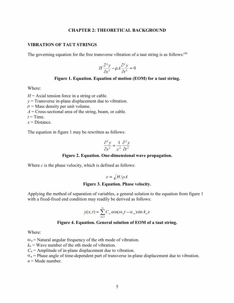
The governing equation for the free transverse vibration of a taut string is as follows:(4)

Figure 1. Equation. Equation of motion (EOM) for a taut string.

Where:

H = Axial tension force in a string or cable. y = Transverse in-plane displacement due to vibration. ρ = Mass density per unit volume. A = Cross-sectional area of the string, beam, or cable. t = Time. x = Distance.

The equation in figure 1 may be rewritten as follows:

Figure 2. Equation. One-dimensional wave propagation.

Where c is the phase velocity, which is defined as follows:

Figure 3. Equation. Phase velocity.

Applying the method of separation of variables, a general solution to the equation from figure 1 with a fixed-fixed end condition may readily be derived as follows:

Figure 4. Equation. General solution of EOM of a taut string.

Where:

n = Natural angular frequency of the nth mode of vibration. kn = Wave number of the nth mode of vibration. Cn = Amplitude of in-plane displacement due to vibration.

n = Phase angle of time-dependent part of transverse in-plane displacement due to vibration. n = Mode number.

ω

α

5

The angular frequencies and wave numbers are not independent of each other but are interrelated as follows:

Figure 5. Equation. Relationship between angular frequency and wave number.

Where:

L = Length of the string.

The equation in figure 4 indicates that the motion of the string is represented by a superposition of standing waves with mode shapes of xknsin and time-varying amplitudes of .

The natural frequencies, n, are the eigenvalues representing the discrete frequencies at which the system is capable of undergoing harmonic motion.

The equation in figure 1 is a linearized EOM in which nonlinearities arising from finite sag are ignored. Note that the only significant parameters in figure 1 through figure 5 are L, H, and A. Also note that from the equation in figure 5, n is proportional to the mode number, n.

From the equations in figure 3 and figure 5, the cable tension H can be determined from the fundamental natural frequency, f, as follows:

Figure 6. Equation. Cable tension.

f, in Hz is related to the angular frequency such that f = /2 .

VIBRATION OF CLASSICAL BEAMS

The governing equation for the free transverse vibration of a Bernoulli-Euler beam is given by the following:(4)

Figure 7. Equation. EOM for a classical beam.

Where:

E = Young’s modulus. I = Moment of inertia.

Cn cos( nt – αn) ω

ω

ρ ω

ω ω π

6

The equation in figure 7 may be rewritten as follows:

Figure 8. Equation. EOM for a classical beam, rewritten with vibration parameter.

Where a is defined as the vibration parameter for classical beam, which can be solved as follows:

Figure 9. Equation. Vibration parameter for a classical beam.

Note that the equation in figure 8 is not of the wave equation form and that a does not have the dimension of velocity. Applying the method of separation of variables, a general solution to the equation in figure 8 with a pinned-pinned end condition can be derived and takes the form of the equation in figure 4, with n and kn being interrelated as follows:

Figure 10. Equation. Relationship between angular frequency and wave number.

The significant parameters in this formulation are L, EI, and A. Note that n ∝ n2.

VIBRATION OF TAUT STRINGS WITH FLEXURAL STIFFNESS

The governing equation for the free transverse vibration of a taut string with flexural rigidity or, equivalently, a classical beam with axial tension, is given by the following equation:

Figure 11. Equation. EOM for a taut string with flexural stiffness.

A general solution to the equation in figure 11 with a pinned-pinned end condition can be derived and again takes the form of the equation in figure 4, with n and kn being interrelated as follows:

Figure 12. Equation. Relationship between angular frequency and wave number for a

string.

ω

ρ ω

ω

7

Or equivalently as follows:

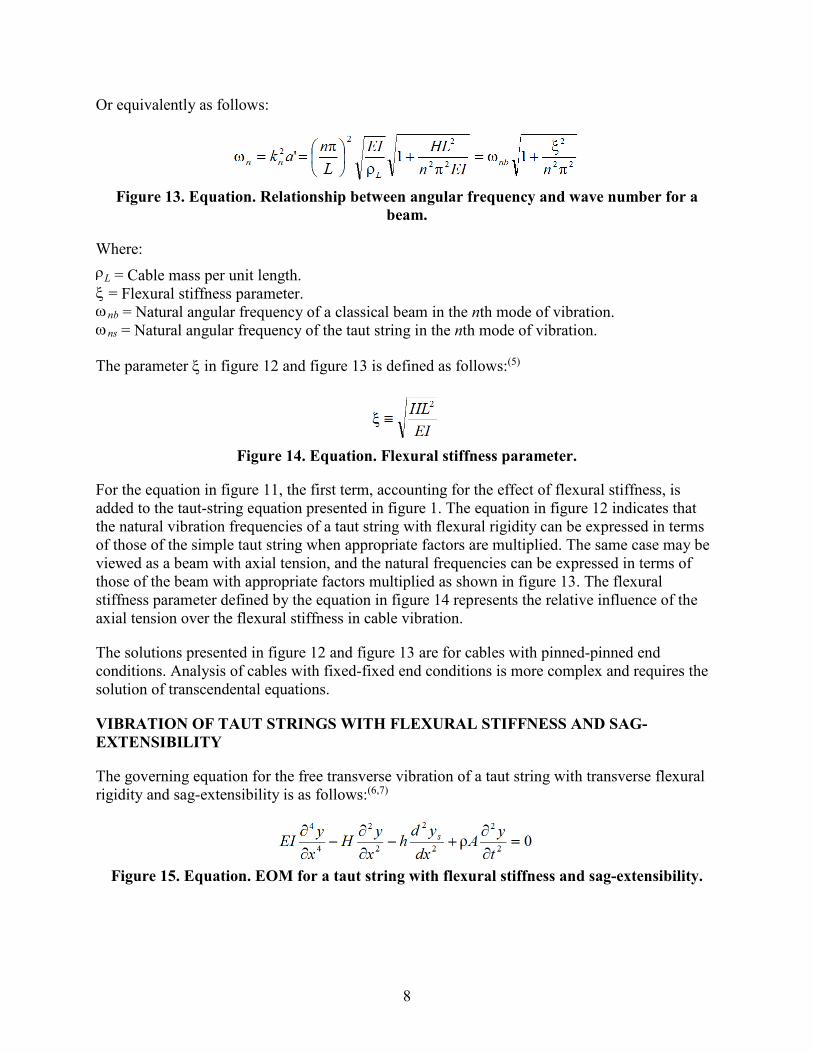
Figure 13. Equation. Relationship between angular frequency and wave number for a

beam.

Where: ρ L = Cable mass per unit length. ξ = Flexural stiffness parameter.

nb = Natural angular frequency of a classical beam in the nth mode of vibration. ns = Natural angular frequency of the taut string in the nth mode of vibration.

The parameter ξ in figure 12 and figure 13 is defined as follows:(5)

Figure 14. Equation. Flexural stiffness parameter.

For the equation in figure 11, the first term, accounting for the effect of flexural stiffness, is added to the taut-string equation presented in figure 1. The equation in figure 12 indicates that the natural vibration frequencies of a taut string with flexural rigidity can be expressed in terms of those of the simple taut string when appropriate factors are multiplied. The same case may be viewed as a beam with axial tension, and the natural frequencies can be expressed in terms of those of the beam with appropriate factors multiplied as shown in figure 13. The flexural stiffness parameter defined by the equation in figure 14 represents the relative influence of the axial tension over the flexural stiffness in cable vibration.

The solutions presented in figure 12 and figure 13 are for cables with pinned-pinned end conditions. Analysis of cables with fixed-fixed end conditions is more complex and requires the solution of transcendental equations.

VIBRATION OF TAUT STRINGS WITH FLEXURAL STIFFNESS AND SAG-EXTENSIBILITY

The governing equation for the free transverse vibration of a taut string with transverse flexural rigidity and sag-extensibility is as follows:(6,7)

Figure 15. Equation. EOM for a taut string with flexural stiffness and sag-extensibility.

ω ω

8

Where:

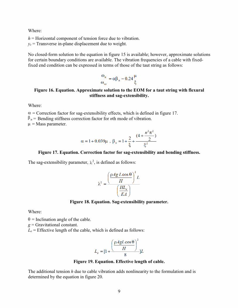
h = Horizontal component of tension force due to vibration. ys = Transverse in-plane displacement due to weight. No closed-form solution to the equation in figure 15 is available; however, approximate solutions for certain boundary conditions are available. The vibration frequencies of a cable with fixed-fixed end condition can be expressed in terms of those of the taut string as follows:

Figure 16. Equation. Approximate solution to the EOM for a taut string with flexural

stiffness and sag-extensibility.

Where: α = Correction factor for sag-extensibility effects, which is defined in figure 17. β n = Bending stiffness correction factor for nth mode of vibration.

= Mass parameter.

Figure 17. Equation. Correction factor for sag-extensibility and bending stiffness.

The sag-extensibility parameter, 2, is defined as follows:

Figure 18. Equation. Sag-extensibility parameter.

Where: θ = Inclination angle of the cable. g = Gravitational constant. Le = Effective length of the cable, which is defined as follows:

Figure 19. Equation. Effective length of cable.

The additional tension h due to cable vibration adds nonlinearity to the formulation and is determined by the equation in figure 20.

µ

λ

9

Figure 20. Equation. Additional tension force due to cable vibration.

The parameter in figure 16 is given by the following:

Figure 21. Equation. Correction factor for sag-extensibility.

The parameter in figure 16 is given by the following:

Figure 22. Equation. Mass parameter.

The two parameters 2 and play a major role in the formulation in figure 14 and figure 15. The relationship of the equation in figure 16 is known to provide a good approximation when 2 < 3 and > 50, and many stay cables in cable-stayed bridges fall within this range.

α

µ

µ = λ2 for n = 1 (in-plane) µ = 0 for n > 1 (in-plane) or for all n (out-of-plane)

λ ξ λ

ξ

10

CHAPTER 3: PRELIMINARY ANALYSIS OF STAY CABLE VIBRATIONS

INTRODUCTION

This chapter illustrates some common issues on finite element analysis of stay cables using examples. First, single cables with varying degrees of complexity were treated. Then, systems with two stay cables interconnected with a transverse crosstie were analyzed. Finally, a stay cable system in an actual cable-stayed bridge that was previously analyzed by other investigators using a non-FEM was analyzed using FEM, and the results were compared.

For analysis, finite element analysis software SAP2000® was used.(8) Beam elements with appropriate properties were used to model the stay cables and crossties, and the P-delta analysis technique was used to account for the effects of pre-tensioned forces in the stay cables and crossties.

NUMERICAL MODELING AND ANALYSIS OF STAY CABLES

Taut String Model

In the first example, the transverse vibration of a stay cable, modeled as a taut string with fixed ends, was analyzed using FEM and compared with the theoretical solution. The cable had the following fictitious properties:

• Length (L) = 1,000 inches (25.4 m).

• Pre-tension (H) = 10 kip (44.5 kN).

• Mass density per unit length (ρ A) = 0.222 lbm/inch (3.96 kg/m), which approximately simulates a steel wire with a diameter (D) of 1 inch (25.4 mm).

A beam element with zero flexural stiffness and subjected to axial tension was used to model a taut string. (In practice, a negligibly small number is used for flexural stiffness to avoid numerical instability.)

An illustration of the cable along with the input data and sample results is presented in figure 23. The results from finite element analysis are shown to match theoretical solutions. T1 and T2 denote the period of the first and second mode, respectively. The first 4 vibration mode shapes calculated are shown in figure 24, and the natural vibration frequencies for the first 10 modes are shown in figure 25. The natural frequency is a linear function of the mode number.

11

Figure 23. Illustration. Analysis of a simple taut string.

Figure 24. Image. The first four mode shapes for the vibration of a taut string.

L= 1000 in, H = 10 kips, ρA = .222 lbm/in

Analysis Results: Theory: T1=0.4797 sec, T2=0.2398 sec FEM: T1=0.4797 sec, T2=0.2399 sec

H EI = 0

12

Figure 25. Graph. Natural vibration frequencies of a taut string.

Classical Beam

The vibration of an Euler-Bernoulli (or classical) beam with hinge-hinge end conditions was analyzed using FEM and compared with theoretical solutions. The beam has the same length and density as the string model discussed previously. The beam is assumed to have a circular cross section with a diameter of 1 inch (25.4 mm) and is made of steel with a Young’s modulus of 2.9E+7 psi (200 GPa).

An illustrative problem with sample input and output data is presented in figure 26. The results from the numerical analysis match the theory. The first 10 natural frequencies are presented in figure 27. The natural frequency of a classical beam is a quadratic function of the mode number, as predicted by the equation in figure 10.

Figure 26. Illustration. Analysis of a classical beam.

0.0

5.0

10.0

15.0

20.0

25.0

0 2 4 6 8 10Mode Number

Freq

uenc

y (H

z)

L= 1000 in, H = 0 kips, ρA = .222 lbm/in, E = 2.9E+7 psi, D = 1 in

Analysis Results:

Theory: T1=12.5805 sec, T2=3.1451 sec FEM: T1=12.5821 sec, T2=3.1455 sec

0 EI

13

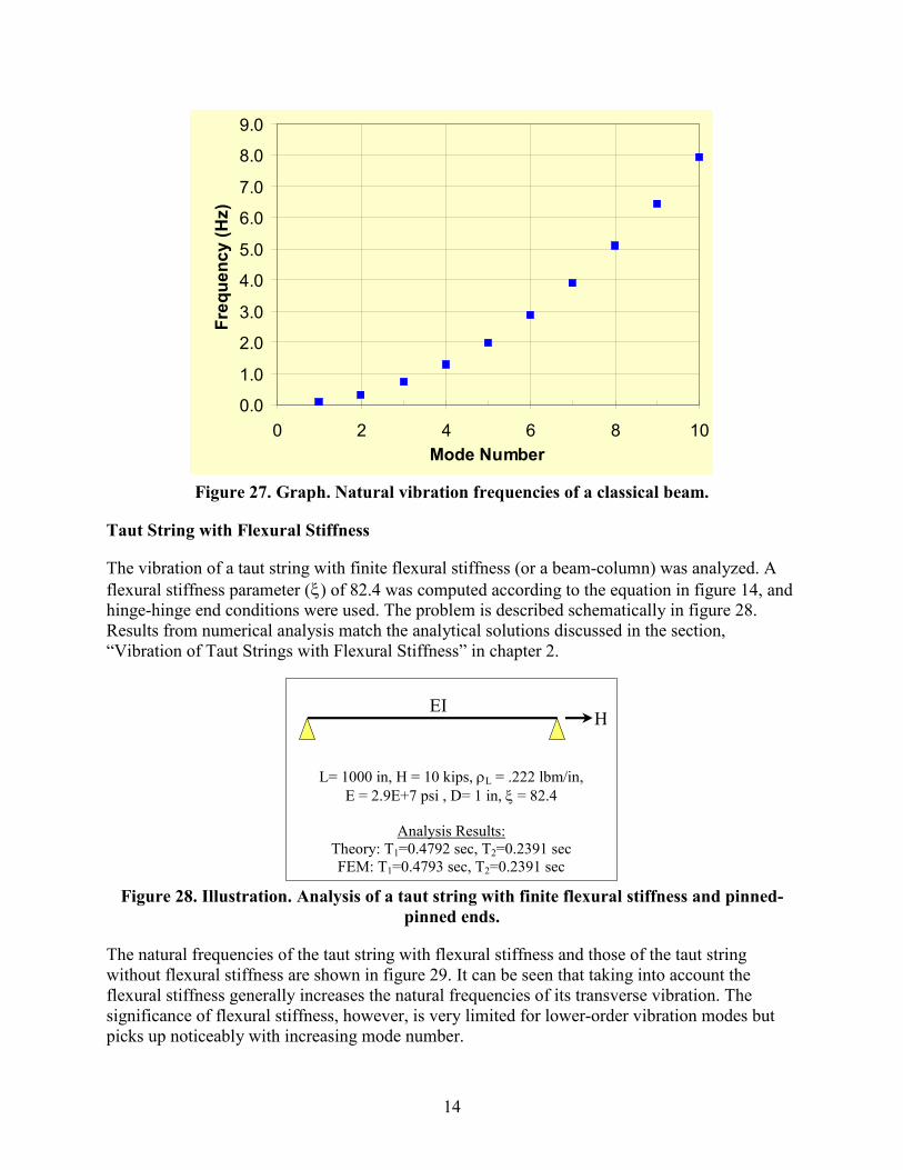
Figure 27. Graph. Natural vibration frequencies of a classical beam.

Taut String with Flexural Stiffness

The vibration of a taut string with finite flexural stiffness (or a beam-column) was analyzed. A flexural stiffness parameter ( ) of 82.4 was computed according to the equation in figure 14, and hinge-hinge end conditions were used. The problem is described schematically in figure 28. Results from numerical analysis match the analytical solutions discussed in the section, “Vibration of Taut Strings with Flexural Stiffness” in chapter 2.

Figure 28. Illustration. Analysis of a taut string with finite flexural stiffness and pinned-

pinned ends.

The natural frequencies of the taut string with flexural stiffness and those of the taut string without flexural stiffness are shown in figure 29. It can be seen that taking into account the flexural stiffness generally increases the natural frequencies of its transverse vibration. The significance of flexural stiffness, however, is very limited for lower-order vibration modes but picks up noticeably with increasing mode number.

0.0

1.0

2.0

3.0

4.0

5.0

6.0

7.0

8.0

9.0


Freq

uenc

y (H

z)

ξ

L= 1000 in, H = 10 kips, ρL = .222 lbm/in, E = 2.9E+7 psi , D= 1 in, ξ = 82.4

Analysis Results:

Theory: T1=0.4792 sec, T2=0.2391 sec FEM: T1=0.4793 sec, T2=0.2391 sec

H EI

14

Figure 29. Graph. Natural vibration frequencies of a taut string with finite flexural

stiffness and hinge-hinge supports.

A similar problem with fixed-end conditions was also analyzed. The finite element solutions match those predicted by an approximate formula by Mehrabi and Tabatabai, as seen in figure 30.(6) No closed form solution is known to exist for this problem.

Figure 30. Illustration. Analysis of a taut string with finite flexural stiffness and fixed-fixed

ends.

In figure 31, the influence of cable end conditions, whether fixed or hinged, on natural frequencies is compared. Relatively small differences are observed between the two cases. However, the differences increase with increasing mode number.

0.0

5.0

10.0

15.0

20.0

25.0


Freq

uenc

y (H

z)

Taut String w/ FlexuralStiffness (hinge-hinge)

Taut String

15

Figure 31. Graph. Natural vibration frequencies of a taut string with finite flexural

stiffness and two different support conditions.

TWO-CABLE SYSTEM WITH CROSSTIE

A simple system of two twin cables interconnected by a cross tie was analyzed (see figure 32). An optional tie to the ground was also considered. Each cable has the same dimensions and properties as the single cable introduced in the previous example (L = 1,000 inches (25.4 m), H = 10 kip (44.5 kN), L = 0.222 lbm/inch (3.96 kg/m), D = 1 inch (25.4 mm), fixed-fixed ends). The ties are modeled as an elastic spring, and a number of combinations of stiffness values (K and KG) are considered, where K is the stiffness between two cables, and KG is the stiffness between the cable and the ground or bridge deck.

Figure 32. Illustration. Two-cable system with crossties.

First, the in-plane free vibration of this system was analyzed. Figure 33 shows the evolution of the natural frequency of a system when K = 0 and KG = 0 (i.e., when there are no crosstie or anchorage connecting the two cables). Figure 34 shows results when K is finite (K = 0.1 kip/inch (7.5 kN/m)) and KG = 0. It can be seen from figure 34 that the frequencies for n = 2, 6, 10, … are increased by the presence of a crosstie (spring) between the cables. Figure 35 shows the evolution of mode-frequencies when both K and KG have finite spring constants.

0.0

5.0

10.0

15.0

20.0

25.0


Freq

uenc

y (H

z)

Taut String w/ FlexuralStiffness (fixed-fixed)

Taut String w/ FlexuralStiffness (hinge-hinge)

ρ

H

H

Ground

K

KG

L/2 L/2

L/2 L/2

16

Figure 33. Graph. Mode-frequency evolution for a two-cable system with K = 0 and KG = 0.

Figure 34. Graph. Mode-frequency evolution for a two-cable system with K = finite and

KG = 0.

Figure 35. Graph. Mode-frequency evolution for a two-cable system with K = finite and

KG = finite.

0.0

2.0

4.0

6.0

8.0

10.0

12.0

14.0


Freq

uenc

y (H

z)

0.0

2.0

4.0

6.0

8.0

10.0

12.0

14.0


Freq

uenc

y (H

z)

0.0

2.0

4.0

6.0

8.0

10.0

12.0

14.0


Freq

uenc

y (H

z)

17

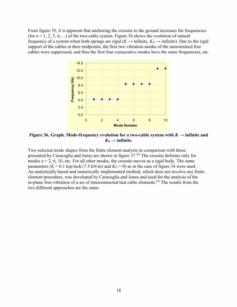
From figure 35, it is apparent that anchoring the crosstie to the ground increases the frequencies (for n = 1, 2, 5, 6,…) of the two-cable system. Figure 36 shows the evolution of natural frequency of a system when both springs are rigid (K → infinite, KG → infinite). Due to the rigid support of the cables at their midpoints, the first two vibration modes of the unrestrained free cables were suppressed, and thus the first four consecutive modes have the same frequencies, etc.

Figure 36. Graph. Mode-frequency evolution for a two-cable system with K → infinite and

KG → infinite.

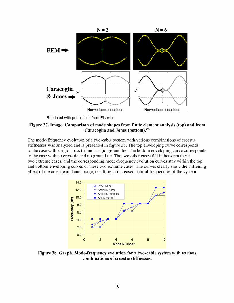
Two selected mode shapes from the finite element analysis in comparison with those presented by Caracoglia and Jones are shown in figure 37.(9) The crosstie deforms only for modes n = 2, 6, 10, etc. For all other modes, the crosstie moves as a rigid body. The same parameters (K = 0.1 kip/inch (7.5 kN/m) and KG = 0) as in the case of figure 34 were used. An analytically based and numerically implemented method, which does not involve any finite element procedure, was developed by Caracoglia and Jones and used for the analysis of the in-plane free-vibration of a set of interconnected taut cable elements.(9) The results from the two different approaches are the same.

0.0

2.0

4.0

6.0

8.0

10.0

12.0

14.0


Freq

uenc

y (H

z)

18

Reprinted with permission from Elsevier

Figure 37. Image. Comparison of mode shapes from finite element analysis (top) and from Caracoglia and Jones (bottom).(9)

The mode-frequency evolution of a two-cable system with various combinations of crosstie stiffnesses was analyzed and is presented in figure 38. The top enveloping curve corresponds to the case with a rigid cross tie and a rigid ground tie. The bottom enveloping curve corresponds to the case with no cross tie and no ground tie. The two other cases fall in between these two extreme cases, and the corresponding mode-frequency evolution curves stay within the top and bottom enveloping curves of these two extreme cases. The curves clearly show the stiffening effect of the crosstie and anchorage, resulting in increased natural frequencies of the system.

Figure 38. Graph. Mode-frequency evolution for a two-cable system with various

combinations of crosstie stiffnesses.

0.0

2.0

4.0

6.0

8.0

10.0

12.0

14.0


Freq

uenc

y (H

z)

K=0, Kg=0K=finite, Kg=0K=finite, Kg=finiteK=inf, Kg=inf

19

FULL-SCALE STAY CABLE NETWORK

Vibration Mode Shapes

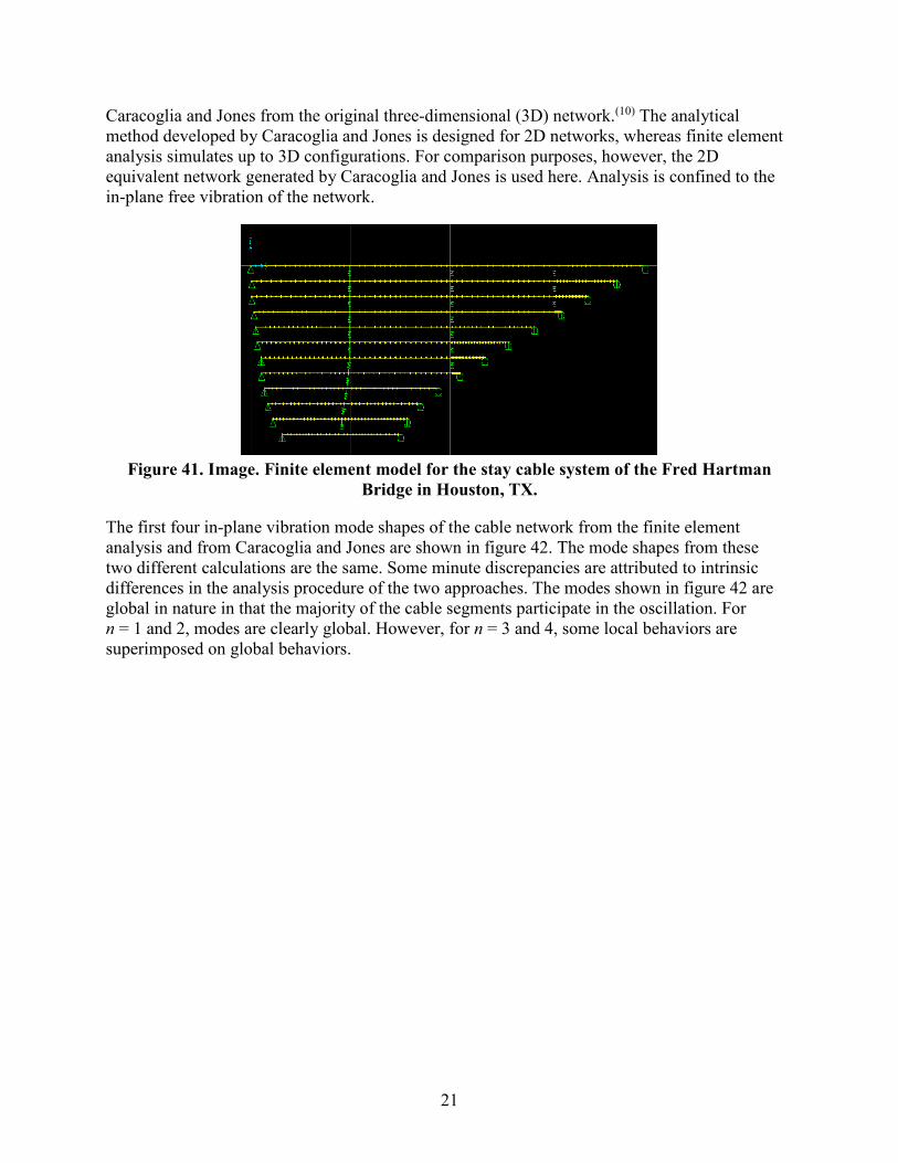
Analysis was extended to a real full-scale cable network. The Fred Hartman Bridge in Houston, TX, was selected for illustration and comparison purposes. Photos of the bridge and cable network are presented in figure 39 and figure 40, respectively. The results from finite element analysis are compared with those from the analytical method by Caracoglia and Jones wherever possible.(10)

Figure 39. Photo. Fred Hartman Bridge in Houston, TX.

Figure 40. Photo. The cable network of the Fred Hartman Bridge in Houston, TX.

Finite element discretization of a network of main-span stay cables (A-line) of the Fred Hartman Bridge is shown in figure 41. The stay cables are interconnected with three lines of crossties. The configuration shown represents an equivalent two-dimensional (2D) network reduced by

20

Caracoglia and Jones from the original three-dimensional (3D) network.(10) The analytical method developed by Caracoglia and Jones is designed for 2D networks, whereas finite element analysis simulates up to 3D configurations. For comparison purposes, however, the 2D equivalent network generated by Caracoglia and Jones is used here. Analysis is confined to the in-plane free vibration of the network.

Figure 41. Image. Finite element model for the stay cable system of the Fred Hartman

Bridge in Houston, TX.

The first four in-plane vibration mode shapes of the cable network from the finite element analysis and from Caracoglia and Jones are shown in figure 42. The mode shapes from these two different calculations are the same. Some minute discrepancies are attributed to intrinsic differences in the analysis procedure of the two approaches. The modes shown in figure 42 are global in nature in that the majority of the cable segments participate in the oscillation. For n = 1 and 2, modes are clearly global. However, for n = 3 and 4, some local behaviors are superimposed on global behaviors.

21


Figure 42. Image. First four vibration mode shapes of the Fred Hartman Bridge stay cable system from finite element analysis (top) and from Caracoglia and Jones (bottom).(10)

As the mode number increases, local modes, in which the response of the network is limited to some intermediate segments of cables, become evident. Figure 43 shows mode shapes for n = 5–8. The wavelengths in these vibration modes are dictated by the distances between two adjacent crossties. Subsequent vibration modes, densely populated in frequency, are seen to be a permutation of a similar pattern dominated by a few cables. Local modes are found to dominate for up to n = 28.

22


Figure 43. Image. Vibration mode shapes 5–8 of the Fred Hartman Bridge stay cable system from finite element analysis (top) and from Caracoglia and Jones (bottom).(10)

However, a second set of global network modes occurred at n = 29 and continued for a few modes and then local modes resumed. This global-local pattern repeats thereafter. Figure 44 shows mode shapes for n = 29–32. Global modes of vibration are noticeable for n = 29–31, and thereafter, local modes resumed.


Figure 44. Image. Vibration mode shapes 29–32 of the Fred Hartman Bridge stay cable system from finite element analysis (top) and from Caracoglia and Jones (bottom).(10)

23

Mode-Frequency Evolution

The modal characteristics of the network are illustrated in figure 45 in the mode-frequency evolution chart where the natural frequency of the network is plotted as a function of the mode number.

Figure 45. Graph. Mode-frequency evolution for the Fred Hartman Bridge stay cable

system from finite element analysis.

The figure shows that a sequence of global modes are followed by a plateau of densely populated local modes, which is then followed by a second set of global modes, etc. This pattern of consecutive steps is typical of the modal behavior of a cable network. Figure 45 shows that the fundamental frequency (n = 1) of the network is bracketed between the fundamental frequencies of the longest and shortest cables. The presence of crossties is seen to enhance the overall performance of the network by increasing their natural frequencies, especially those of global modes. However, analysis also suggests that the presence of crossties may not necessarily be beneficial at plateau frequencies due to potentially undesirable effects associated with densely populated local modes.

The mode-frequency evolution chart generated by Caracoglia and Jones is presented in figure 46 for comparison.(10) The finite element results presented in figure 45 correspond to their analysis case, “NET_3C.” Overall, the results from both approaches are the same.


0.51.01.52.02.53.03.54.04.5

0 5 10 15 20 25 30 35Mode Number

Freq

uenc

y (H

z)NETWORKLongest CableShortest Cable

24


Figure 46. Graph. Mode-frequency evolution for the Fred Hartman Bridge stay cable system.(10)

Variations in Crosstie Configuration

As a modification to the original configuration, two shorter crossties were tied to the ground (i.e., the deck), as shown in figure 47. The resulting mode shapes (for n = 1 and 2) are presented in figure 48. The first mode is quite similar to that of the previous (reference) network. However, the second mode is rather different from the case of the reference network due to anchoring of the middle line of crosstie.

Figure 47. Image. Finite element model for the stay cable system with some crossties

anchored to the deck.

25


Figure 48. Image. First two vibration mode shapes for the model shown in figure 47 from finite element analysis (top) and from Caracoglia and Jones (bottom).(10)

The effect of crosstie anchoring was examined in terms of the mode-frequency evolution behavior, which is shown in figure 49. The addition of grounding ties significantly increased the frequencies of global modes but did not increase the frequencies of local modes by a significant amount. Grounding of crossties apparently made the network stiffer with respect to its global behavior, but it practically did not affect the local vibration responses of individual cables.

Figure 49. Graph. Comparison of mode-frequency evolution for models shown in figure 41

(reference) and figure 47.

As another fictitious variation to the original configuration, the geometry of the two shorter restrainers was modified, as shown in figure 50. This modification helps avoid excessive stretch


0.5

1.0

1.5

2.0

2.5

3.0

3.5

4.0

4.5

0 5 10 15 20 25 30 35Mode Number

Freq

uenc

y (H

z)

NETWORK (Reference)NETWORK w/ 2 Ground Ties

26

of the segments of some cables due to the grounding of crossties. This modification would avoid undesirable stress concentrations in these cable segments.

Figure 50. Image. Finite element model for the stay cable system with a varied crosstie

configuration (variation 1).

The first four vibration mode shapes for this variation are shown in figure 51, and the mode-frequency evolution is shown in figure 52. This variation renders slightly lower frequencies of global modes and yet somewhat higher frequencies of local modes. The step behavior of the original configuration is slightly rounded. Comparing figure 51 with figure 42 suggests an improvement of this variation over the original configuration by avoiding the presence of very short segments of cables.

Figure 51. Image. Vibration mode shapes 1–4 for the model shown in figure 50.

NN == 11 NN == 22

NN == 33 NN == 44

27



The third variation to the original crosstie configuration involves only a single line of crossties as shown in figure 53. Figure 54 shows the first four mode shapes of this variation, and figure 55 shows the corresponding mode-frequency evolution (in solid diamonds) in contrast to that of the reference configuration. Clearly, it can be seen that the single line of crossties provides less reinforcement to the cable system. More frequent global-local steps occur as the quantity of crossties is reduced.

Figure 53. Image. Finite element model for the stay cable system with a single crosstie line

(variation 2).


0.5

1.0

1.5

2.0

2.5

3.0

3.5

4.0

4.5

0 5 10 15 20 25 30 35Mode Number

Freq

uenc

y (H

z)

NETWORK (Reference)Network - Variation #1

28

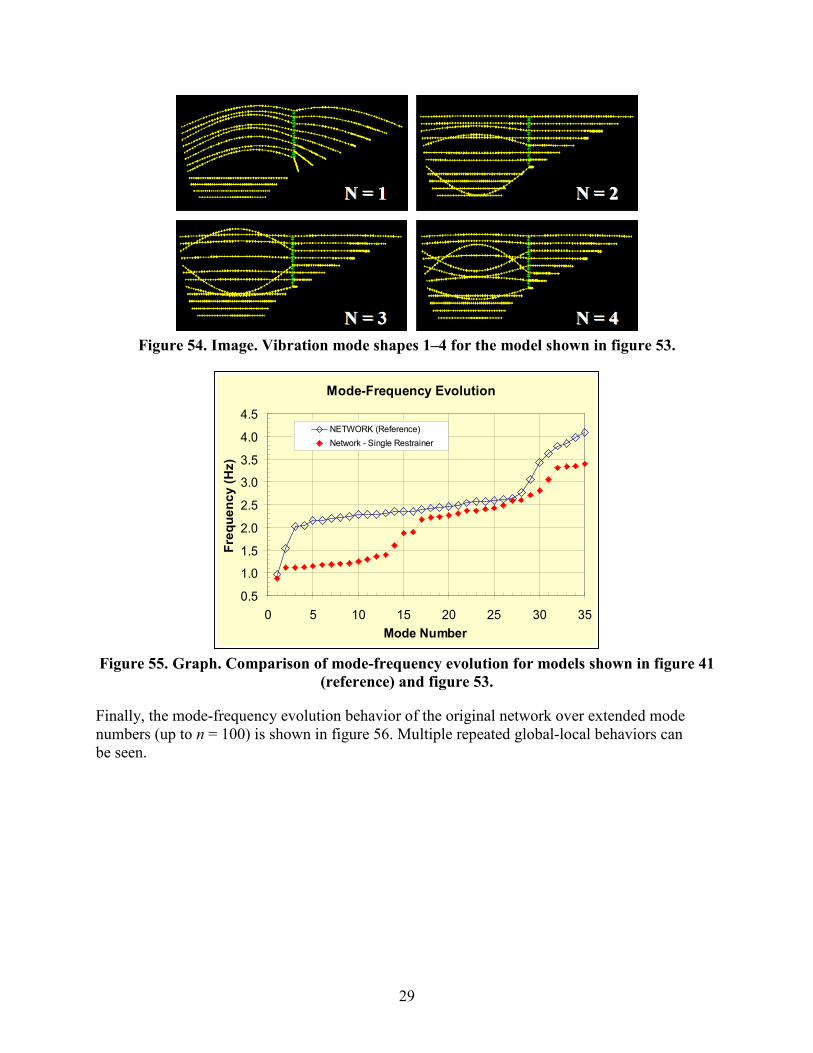
Figure 54. Image. Vibration mode shapes 1–4 for the model shown in figure 53.



Finally, the mode-frequency evolution behavior of the original network over extended mode numbers (up to n = 100) is shown in figure 56. Multiple repeated global-local behaviors can be seen.


0.5

1.0

1.5

2.0

2.5

3.0

3.5

4.0

4.5

0 5 10 15 20 25 30 35Mode Number

Freq

uenc

y (H

z)

NETWORK (Reference)Network - Single Restrainer

29

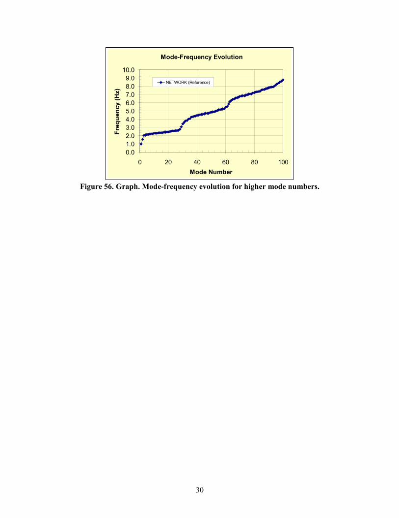
Figure 56. Graph. Mode-frequency evolution for higher mode numbers.


0.01.02.03.04.05.06.07.08.09.0

10.0

0 20 40 60 80 100Mode Number

Freq

uenc

y (H

z)

NETWORK (Reference)

30

CHAPTER 4: FREE-VIBRATION ANALYSIS OF STAY CABLE SYSTEMS WITH CROSSTIES

INTRODUCTION

The in-plane stiffness of stay cables increases when they are connected by means of a set of transverse cables referred to as “crossties.” Crossties have been introduced over the past several decades as a means of counteracting large-amplitude vibrations of the stays in cable-stayed bridges. Crossties are also known to reduce the cable sag variations among stay cables of various lengths.(11) From the dynamics point of view, the presence of lateral constraints modifies the oscillation characteristics of the stay group. Also, the interconnection of individual stay cables results in a complex cable network. As a result, a closed-form solution to a structural analysis problem of such network is elusive.

A number of studies on crossties for stay cables have been conducted. (See references 9, 10, 12, and 13). However, the dynamic behavior of a stay cable system networked with crossties is still not clearly understood, and the effectiveness of crossties is not well established. In this study, the effectiveness of crossties in mitigation of stay cable vibrations was numerically investigated. Both modal analyses and time-history analyses were conducted on a set of stay cables from the recently completed Bill Emerson Memorial Bridge in Cape Girardeau, MO. The modal (i.e., free-vibration) analysis is discussed later in this chapter. The time-history (i.e., forced-vibration) analysis under transient wind loads is discussed in chapter 5.

Numerical analysis was conducted using the general purpose finite element code SAP2000®.(8)

An elevation view of the subject bridge is shown in figure 57 with the cables under study circled in blue. The bridge has two H-shaped towers supporting 128 stays. The main span of the bridge is 1,148 ft (350 m) long, and two side spans are each 468 ft (143 m) long. The finite element discretization of a side section of stay cables is shown in figure 58. Four parallel lines of crossties perpendicular to the longest cable and equally dividing this cable into five segments are considered as the reference configuration. A few other configurations of crossties are also considered later for comparison purposes. The basic information on the bridge, as provided by the designer, is presented in table 1. Data on cable-end coordinates and cable properties are presented in table 2 and table 3.

31

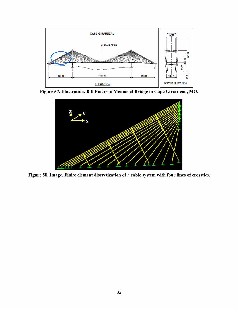
Figure 57. Illustration. Bill Emerson Memorial Bridge in Cape Girardeau, MO.

Figure 58. Image. Finite element discretization of a cable system with four lines of crossties.

32

Table 1. Basic information on the Bill Emerson Memorial Bridge. Bridge Name Cape Girardeau/Bill Emerson Memorial Owner State of Missouri Designer HNTB Year Design Completed 1996 Year Construction Completed 2003 Superstructure Type Steel composite Superstructure Width 96 ft (29.26 m) Tower Type H-shaped Main Span Length 1,150 ft (350.52 m) Side Span Length 468 ft (142.65 m) Number of Stays 128 Number of Stay Planes 2 Cable Type Seven-wire strand Strand Diameter 0.62 inch (1.52 cm) Grout Cement Outer Sheathing High-density polyethylene Supplemental UV Protection None Number of Cross Tie Lines—Side Span 4 Number of Cross Tie Lines—Main Span 4 Crosstie Diameter 0.81 inch (2.06 cm) Supplemental Damper Neoprene Damper Location Both ends

33

Table 2. Coordinates of cable ends on the Bill Emerson Memorial Bridge.

Cable Number

Tower-End X-Coordinate

(ft)

Tower-End Z-Coordinate

(ft)

Deck-End X-Coordinate

(ft)

Deck-End Z-Coordinate

(ft) 1 -5.77 310.3 -460.6 66.0 2 -5.77 305.3 -448.6 66.5 3 -5.77 300.3 -436.6 66.9 4 -5.77 295.3 -424.7 67.3 5 -5.77 290.2 -413.1 67.6 6 -5.74 285.3 -378.4 68.8 7 -5.67 280.4 -343.8 70.0 8 -5.64 275.4 -309.2 71.3 9 -5.67 270.5 -274.8 72.5 10 -5.61 265.6 -240.3 73.7 11 -5.61 260.7 -205.8 75.0 12 -5.97 255.4 -171.3 76.3 13 -6.04 249.4 -137.1 77.4 14 -6.04 242.7 -102.7 78.7 15 -7.71 230.8 -68.4 79.9 16 -7.77 213.5 -34.1 81.4

1 ft = 0.305 m

34

Table 3. Cable properties on the Bill Emerson Memorial Bridge.

Cable No.

Chord Length

(ft)

Outer Diameter

(inch)

Young's Modulus (106 psi)

Cable Tension

(kip)

Mass Density (lbm/ft3)

Unit Weight (lbf/ft3)

Unit Weight

per Length (lbf/ft)

Frequency String Theory

(Hz) 1 516.3 10.75 2.261 1019.6 162.1 162.1 102.1 0.549 2 503.1 10.75 2.261 1069.4 162.1 162.1 102.1 0.577 3 490.0 10.75 2.180 1019.6 159.0 159.0 100.1 0.584 4 476.9 8.62 2.768 979.6 172.7 172.7 70.0 0.703 5 464.2 8.62 2.621 935.5 170.5 170.5 69.1 0.711 6 431.0 8.62 2.523 901.3 168.0 168.0 68.1 0.758 7 398.2 8.62 2.425 855.5 168.0 168.0 68.1 0.799 8 365.8 8.62 2.425 827.4 168.0 168.0 68.1 0.855 9 334.1 7.12 3.564 735.3 180.6 180.6 50.0 1.029 10 303.1 7.12 3.444 672.4 177.0 177.0 49.0 1.095 11 273.1 7.12 3.324 636.4 173.4 173.4 48.0 1.196 12 243.7 7.12 3.204 591.2 169.8 169.8 47.0 1.305 13 216.3 6.61 2.789 561.3 171.9 171.9 41.0 1.534 14 190.3 6.61 2.468 463.1 167.7 167.7 40.0 1.603 15 169.1 6.61 2.307 409.2 163.5 163.5 39.0 1.718 16 147.7 6.61 2.227 380.2 163.5 163.5 39.0 1.894

1 ft = 0.305 m 1 inch = 25.4 mm 1 psi = 6.89 kPa 1 kip = 4.45 kN 1 lbm/ft3 = 16.0 kg/m3 1 lbf/ft3 = 0.157 kN/m3 1 lbf/ft = 0.0146 kN/m

The stay cables and crossties are modeled using the beam elements with their flexural stiffness. The pre-tension forces in stay cables and crossties are modeled using P-delta forces. The cable ends are assumed to be fixed to the deck and to the tower. Both the deck and the tower are assumed to be immobile relative to the stays for simplicity, and no parametric motion between the stays and the deck or tower is considered. Analysis is also focused on the in-plane motion of the stay system, with the out-of-plane motion being treated as an exception.

NATURAL FREQUENCIES AND MODE SHAPES

Free-vibration analysis of a structural system provides information on the system’s intrinsic vibration characteristics commonly expressed in terms of natural frequencies and the corresponding mode shapes. A set of homogeneous dynamic equilibrium equations for a system leads to an eigenvalue problem in which the eigenvalues are identified as the system’s natural vibration frequencies and the corresponding eigenvectors as the mode shapes. A change in structural condition causes changes in the natural frequencies and mode shapes. Therefore, the

35

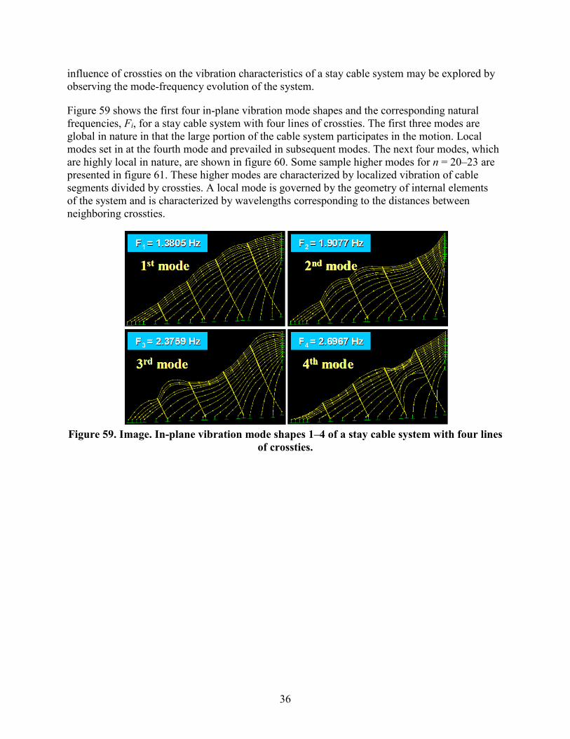
influence of crossties on the vibration characteristics of a stay cable system may be explored by observing the mode-frequency evolution of the system.

Figure 59 shows the first four in-plane vibration mode shapes and the corresponding natural frequencies, Fi, for a stay cable system with four lines of crossties. The first three modes are global in nature in that the large portion of the cable system participates in the motion. Local modes set in at the fourth mode and prevailed in subsequent modes. The next four modes, which are highly local in nature, are shown in figure 60. Some sample higher modes for n = 20–23 are presented in figure 61. These higher modes are characterized by localized vibration of cable segments divided by crossties. A local mode is governed by the geometry of internal elements of the system and is characterized by wavelengths corresponding to the distances between neighboring crossties.

Figure 59. Image. In-plane vibration mode shapes 1–4 of a stay cable system with four lines

of crossties.

36

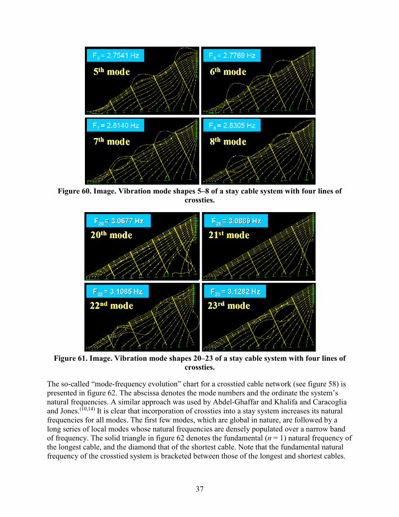
Figure 60. Image. Vibration mode shapes 5–8 of a stay cable system with four lines of

crossties.

Figure 61. Image. Vibration mode shapes 20–23 of a stay cable system with four lines of

crossties.

The so-called “mode-frequency evolution” chart for a crosstied cable network (see figure 58) is presented in figure 62. The abscissa denotes the mode numbers and the ordinate the system’s natural frequencies. A similar approach was used by Abdel-Ghaffar and Khalifa and Caracoglia and Jones.(10,14) It is clear that incorporation of crossties into a stay system increases its natural frequencies for all modes. The first few modes, which are global in nature, are followed by a long series of local modes whose natural frequencies are densely populated over a narrow band of frequency. The solid triangle in figure 62 denotes the fundamental (n = 1) natural frequency of the longest cable, and the diamond that of the shortest cable. Note that the fundamental natural frequency of the crosstied system is bracketed between those of the longest and shortest cables.

37

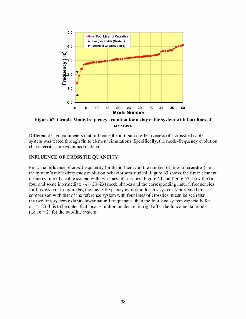
Figure 62. Graph. Mode-frequency evolution for a stay cable system with four lines of

crossties.

Different design parameters that influence the mitigation effectiveness of a crosstied cable system was tested through finite element simulations. Specifically, the mode-frequency evolution characteristics are examined in detail.

INFLUENCE OF CROSSTIE QUANTITY

First, the influence of crosstie quantity (or the influence of the number of lines of crossties) on the system’s mode-frequency evolution behavior was studied. Figure 63 shows the finite element discretization of a cable system with two lines of crossties. Figure 64 and figure 65 show the first four and some intermediate (n = 20–23) mode shapes and the corresponding natural frequencies for this system. In figure 66, the mode-frequency evolution for this system is presented in comparison with that of the reference system with four lines of crossties. It can be seen that the two line-system exhibits lower natural frequencies than the four-line system especially for n = 4–23. It is to be noted that local vibration modes set in right after the fundamental mode (i.e., n = 2) for the two-line system.

0.0

1.0

2.0

3.0

4.0

5.0

0 5 10 15 20 25 30 35 40 45 50Mode Number

Freq

uenc

y (H

z)

w/ Four Lines of CrosstiesLongest Cable (Mode 1)Shortest Cable (Mode 1)

38

Figure 63. Image. Finite element discretization of a cable system with two lines of crossties.

Figure 64. Image. Vibration mode shapes 1–4 of a stay cable system with two lines of

crossties.

39

Figure 65. Image. Vibration mode shapes 20–23 of a stay cable system with two lines of

crossties.

Figure 66. Graph. Mode-frequency evolution for a stay cable system with two lines of

crossties.

Figure 67 shows the finite element discretization of a cable system with a single line of crossties. Figure 68 and figure 69 show the first four and some intermediate mode shapes (n = 20–23) and the corresponding natural frequencies for this system. The system’s mode-frequency evolution behavior is shown in figure 70. Again, the behavior of the reference (four-line) system is presented for comparison. The one-line system exhibits much lower natural frequencies than the reference system. It is difficult to distinguish global modes from local modes, and local modes appear to set in at the very first mode.

0.0

1.0

2.0

3.0

4.0

5.0

0 5 10 15 20 25 30 35 40 45 50Mode Number

Freq

uenc

y (H

z)

w/ Two Lines of Crossties

w/ Four Lines of Crossties

40

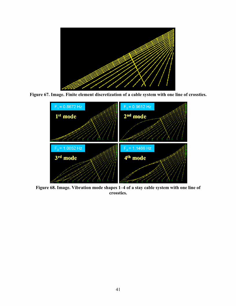
Figure 67. Image. Finite element discretization of a cable system with one line of crossties.

Figure 68. Image. Vibration mode shapes 1–4 of a stay cable system with one line of

crossties.

41


crossties.

Figure 70. Graph. Mode-frequency evolution for a stay cable system with one line of

crossties.

A cable system without any crossties was also considered, and its finite element discretization is shown in figure 71. The first four mode shapes and some intermediate mode shapes (n = 20–23) for this system are shown in figure 72 and figure 73. For a cable system without crossties, the natural modes of the system consist of the natural modes of the individual cables. The first few system modes correspond to the fundamental modes of individual cables. However, at some point, higher modes of long cables begin to interlace with lower modes of short cables. The mode-frequency evolution behavior is shown in figure 74 along with that of the reference four-line system. Again, the efficiency of crossties in terms of enhancing the system’s natural frequencies is evident. The presence of step jumps in mode-frequency chart, which is characteristics of crosstied cable systems, is not seen in the case of the non-crosstied system.

0.0

1.0

2.0

3.0

4.0

5.0

0 5 10 15 20 25 30 35 40 45 50Mode Number

Freq

uenc

y (H

z)

w/ Single Line of Crossties


42

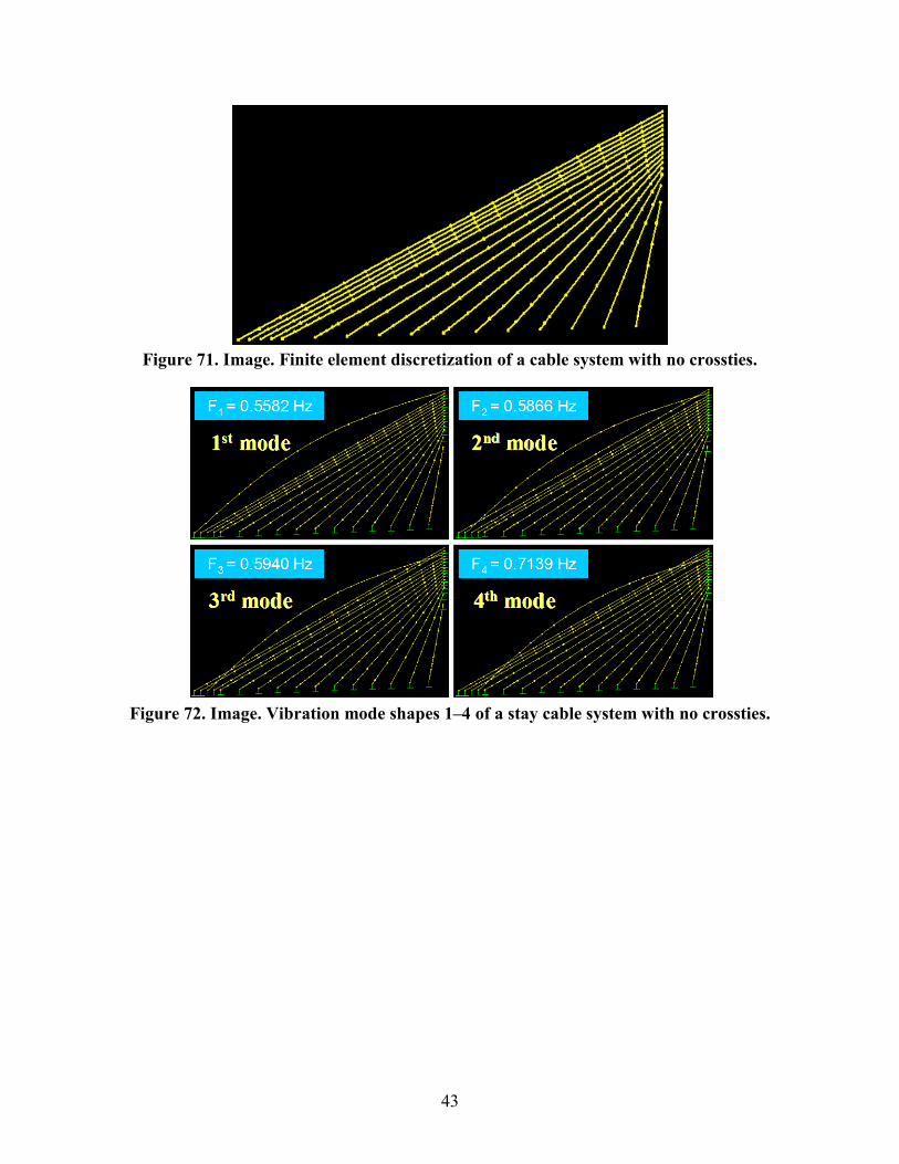
Figure 71. Image. Finite element discretization of a cable system with no crossties.

Figure 72. Image. Vibration mode shapes 1–4 of a stay cable system with no crossties.

43

Figure 73. Image. Vibration mode shapes 20–23 of a stay cable system with no crossties.

Figure 74. Graph. Mode-frequency evolution for a stay cable system with no crossties.

Another simulation was conducted with nine lines of crossties. Figure 75 shows the finite element discretization of a cable system with nine parallel lines of crossties. Figure 76 and figure 77 show the mode shapes for this system, n = 1–4 and n = 20–23. The mode-frequency evolution is presented in figure 78 as a comparison to the reference system. Distinction between global and local modes is clear; however, modes up to n = 25 generally engage a large portion of the segments and thus may be global in nature. A plateau of densely populated local modes appears at a much higher mode compared to the reference four-line system.

0.0

1.0

2.0

3.0

4.0

5.0

0 5 10 15 20 25 30 35 40 45 50Mode Number

Freq

uenc

y (H

z)

w/ No Crossties


44

Figure 75. Image. Finite element discretization of a cable system with nine lines of crossties.

Figure 76. Image. Vibration mode shapes 1–4 of a stay cable system with nine lines of

crossties.

45

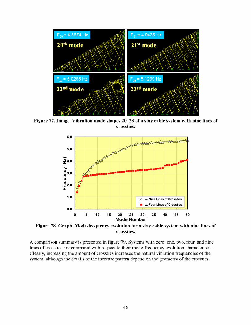
Figure 77. Image. Vibration mode shapes 20–23 of a stay cable system with nine lines of

crossties.

Figure 78. Graph. Mode-frequency evolution for a stay cable system with nine lines of

crossties.

A comparison summary is presented in figure 79. Systems with zero, one, two, four, and nine lines of crossties are compared with respect to their mode-frequency evolution characteristics. Clearly, increasing the amount of crossties increases the natural vibration frequencies of the system, although the details of the increase pattern depend on the geometry of the crossties.

0.0

1.0

2.0

3.0

4.0

5.0

6.0

0 5 10 15 20 25 30 35 40 45 50Mode Number

Freq

uenc

y (H

z)

w/ Nine Lines of Crossties


46

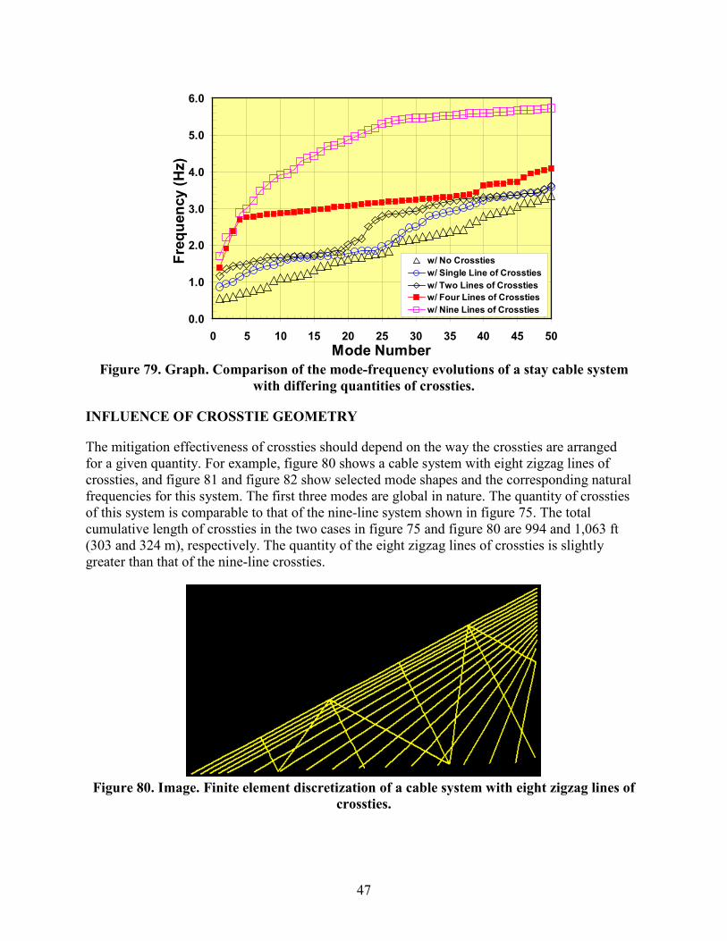
Figure 79. Graph. Comparison of the mode-frequency evolutions of a stay cable system

with differing quantities of crossties.

INFLUENCE OF CROSSTIE GEOMETRY

The mitigation effectiveness of crossties should depend on the way the crossties are arranged for a given quantity. For example, figure 80 shows a cable system with eight zigzag lines of crossties, and figure 81 and figure 82 show selected mode shapes and the corresponding natural frequencies for this system. The first three modes are global in nature. The quantity of crossties of this system is comparable to that of the nine-line system shown in figure 75. The total cumulative length of crossties in the two cases in figure 75 and figure 80 are 994 and 1,063 ft (303 and 324 m), respectively. The quantity of the eight zigzag lines of crossties is slightly greater than that of the nine-line crossties.

Figure 80. Image. Finite element discretization of a cable system with eight zigzag lines of

crossties.

0.0

1.0

2.0

3.0

4.0

5.0

6.0

0 5 10 15 20 25 30 35 40 45 50Mode Number

Freq

uenc

y (H

z)

w/ No Crosstiesw/ Single Line of Crosstiesw/ Two Lines of Crosstiesw/ Four Lines of Crosstiesw/ Nine Lines of Crossties

47

Figure 81. Image. Vibration mode shapes 1–4 of a stay cable system with eight zigzag lines

of crossties.

Figure 82. Image. Vibration mode shapes 20–23 of a stay cable system with eight zigzag

lines of crossties.

The mode-frequency evolution for this system is presented in figure 83. Also presented for comparison are those for the four-line and the eight-line systems. For comparable crosstie quantities, the straight-line (nine lines) system yields much higher natural frequencies than the zigzag (eight lines) system, especially at higher modes (i.e., n > 5). Note that the zigzag arrangement constitutes a larger quantity than the straight-line arrangement. It can also be seen that the straight line arrangement shifts the band of densely populated local modes to a much higher mode.

48

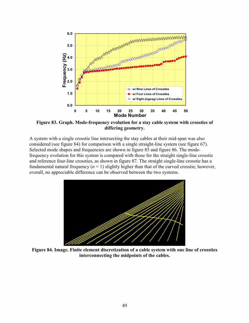
Figure 83. Graph. Mode-frequency evolution for a stay cable system with crossties of

differing geometry.

A system with a single crosstie line intersecting the stay cables at their mid-span was also considered (see figure 84) for comparison with a single straight-line system (see figure 67). Selected mode shapes and frequencies are shown in figure 85 and figure 86. The mode-frequency evolution for this system is compared with those for the straight single-line crosstie and reference four-line crossties, as shown in figure 87. The straight single-line crosstie has a fundamental natural frequency (n = 1) slightly higher than that of the curved crosstie; however, overall, no appreciable difference can be observed between the two systems.

Figure 84. Image. Finite element discretization of a cable system with one line of crossties

interconnecting the midpoints of the cables.

0.0

1.0

2.0

3.0

4.0

5.0

6.0

0 5 10 15 20 25 30 35 40 45 50Mode Number

Freq

uenc

y (H

z)

w/ Nine Lines of Crosstiesw/ Four Lines of Crosstiesw/ Eight (zigzag) Lines of Crossties

49


crossties interconnecting the cable midpoints.


crossties interconnecting the cable midpoints.

50

Figure 87. Graph. Mode-frequency evolution for a stay cable system with one line of

crossties of differing geometry.

INFLUENCE OF CROSSTIE DIAMETER

The influence of crosstie size (or diameter) on the in-plane vibration behavior of a crosstied stay system was investigated. Figure 88 shows fundamental vibration modes (n = 1) for a four-line system with different crosstie diameters that are 0.5, 1.0, 2.0, and 10.0 times the diameter of the reference crosstie. The mode-frequency evolutions for these four different cases are presented in figure 89.

Figure 88. Image. Fundamental vibration mode of a stay cable system with four lines of

crossties of differing diameter.

0.0

1.0

2.0

3.0

4.0

5.0

0 5 10 15 20 25 30 35 40 45 50Mode Number

Freq

uenc

y (H

z)

w/ Single Line of Crosstiesw/ Four Lines of Crosstiesw/ Single Line of Crossties through Cable Midpoints

51

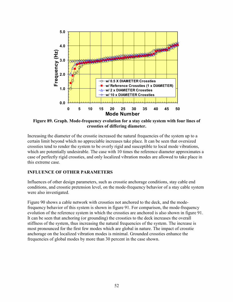
Figure 89. Graph. Mode-frequency evolution for a stay cable system with four lines of

crossties of differing diameter.

Increasing the diameter of the crosstie increased the natural frequencies of the system up to a certain limit beyond which no appreciable increases take place. It can be seen that oversized crossties tend to render the system to be overly rigid and susceptible to local mode vibrations, which are potentially undesirable. The case with 10 times the reference diameter approximates a case of perfectly rigid crossties, and only localized vibration modes are allowed to take place in this extreme case.

INFLUENCE OF OTHER PARAMETERS

Influences of other design parameters, such as crosstie anchorage conditions, stay cable end conditions, and crosstie pretension level, on the mode-frequency behavior of a stay cable system were also investigated.

Figure 90 shows a cable network with crossties not anchored to the deck, and the mode-frequency behavior of this system is shown in figure 91. For comparison, the mode-frequency evolution of the reference system in which the crossties are anchored is also shown in figure 91. It can be seen that anchoring (or grounding) the crossties to the deck increases the overall stiffness of the system, thus increasing the natural frequencies of the system. The increase is most pronounced for the first few modes which are global in nature. The impact of crosstie anchorage on the localized vibration modes is minimal. Grounded crossties enhance the frequencies of global modes by more than 30 percent in the case shown.

0.0

1.0

2.0

3.0

4.0

5.0

0 5 10 15 20 25 30 35 40 45 50Mode Number

Freq

uenc

y (H

z)

w/ 0.5 X DIAMETER Crosstiesw/ Reference Crossties (1 x DIAMETER)w/ 2 x DIAMETER Crosstiesw/ 10 x DIAMETER Crossties

52

Figure 90. Image. Finite element discretization of a cable system with four lines of crossties

not anchored to the deck.

Figure 91. Graph. Effect of crosstie anchorage (to the deck) on the mode-frequency

evolution of a stay cable system with four lines of crossties.

Figure 92 shows the influence of stay cable end conditions on the modal characteristics of a cable network. The figure shows that end conditions, whether fixed or hinged, do not affect the system’s modal behavior that much, except for very high vibration modes. As the mode number increases, the vibration wavelength becomes shorter, and the cable support conditions become increasingly significant.

0.0

1.0

2.0

3.0

4.0

5.0

0 5 10 15 20 25 30 35 40 45 50Mode Number

Freq

uenc

y (H

z)

w/ Crossties Grounded (Reference)w/ Crossties not Grounded

53

Figure 92. Graph. Effect of cable end conditions on the mode-frequency evolution of a stay

cable system with four lines of crossties.

Figure 93 shows the sensitivity of the mode-frequency behavior of a system to pre-tension level in the crossties. The open circles denote the case of reference tension level, while the small closed circles denote the case of 10 times the reference pre-tension level. The two lines shown practically overlap entirely, and virtually no influence of pre-tension level can be observed. Pre-tension affects the transverse (or flexural) stiffness of crossties and the in-plane vibration of a cable network is not much sensitive to the transverse stiffness of crossties. However, crossties must be provided with appropriate levels of pre-tension to prevent slack of the crossties during design wind events. The analysis showed that as long as adequate levels of pre-tension are maintained, the pre-tension does not affect the system’s in-plane vibration behavior. Conversely, the transverse (i.e., out-of-plane) vibration is affected significantly by the pre-tension level, as is discussed in the following section.

Figure 93. Graph. Effect of crosstie tension on the mode-frequency evolution of a stay cable

system with four lines of crossties.

0.0

1.0

2.0

3.0

4.0

5.0

0 5 10 15 20 25 30 35 40 45 50Mode Number

Freq

uenc

y (H

z)

Analysis w/ Fixed Ends (Reference)Analysis w/ Hinged Ends

0.0

1.0

2.0

3.0

4.0

5.0

0 5 10 15 20 25 30 35 40 45 50Mode Number

Freq

uenc

y (H

z)

w/ 1 x Crosstie Tension (Reference)

w/ 10 x Crosstie Tension

54

OUT-OF-PLANE BEHAVIOR

It is well known that crossties are not effective in mitigation of out-of-plane vibration of stay cables due to their limited flexural stiffnesses. This fact and other related issues were verified through finite element analysis. The first four transverse vibration mode shapes and natural frequencies are presented in figure 94. Although crossties are not primarily designed to counteract the transverse vibrations of stay cables, they still provide some limited constraints to transverse vibrations.

Figure 94. Image. Transverse vibration mode shapes 1–4 of a stay cable system with four

lines of crossties.

Figure 95 compares the transverse mode-frequency behavior of stay systems with and without crossties. It confirms the notion that crossties are ineffective in providing transverse constraints to a crosstied cable network. Very limited increases in natural frequency were observed. Figure 96 shows the influence of pre-tension level in crossties on the transverse vibration of stays. While the pre-tension level practically does not affect the in-plane behavior, it affects the out-of-plane behavior. Increased pre-tension leads to increased system frequency, which can be understood from the fact that increased pre-tension increases the flexural stiffness of the system.

F3 = 0.7326 Hz

F1 = 0.5790 Hz F2 = 0.6499 Hz

F4 = 0.7775 Hz

11stst modemode 22ndnd modemode

33rdrd modemode 44thth modemode

55

Figure 95. Graph. Transverse mode-frequency evolution for a stay cable system with and

without crossties.

Figure 96. Graph. Effect of cable tension on the transverse mode-frequency evolution for a

stay cable system with four lines of crossties.

0.0

1.0

2.0

3.0

4.0

5.0

0 5 10 15 20 25 30 35 40 45 50Mode Number

Freq

uenc

y (H

z)

w/ Four Lines of Crosstiesw/ No Crossties

0.0

1.0

2.0

3.0

4.0

5.0

0 5 10 15 20 25 30 35 40 45 50Mode Number

Freq

uenc

y (H

z)

w/ 1 x Crosstie Tension (Reference)

w/ 10 x Crosstie Tension

56

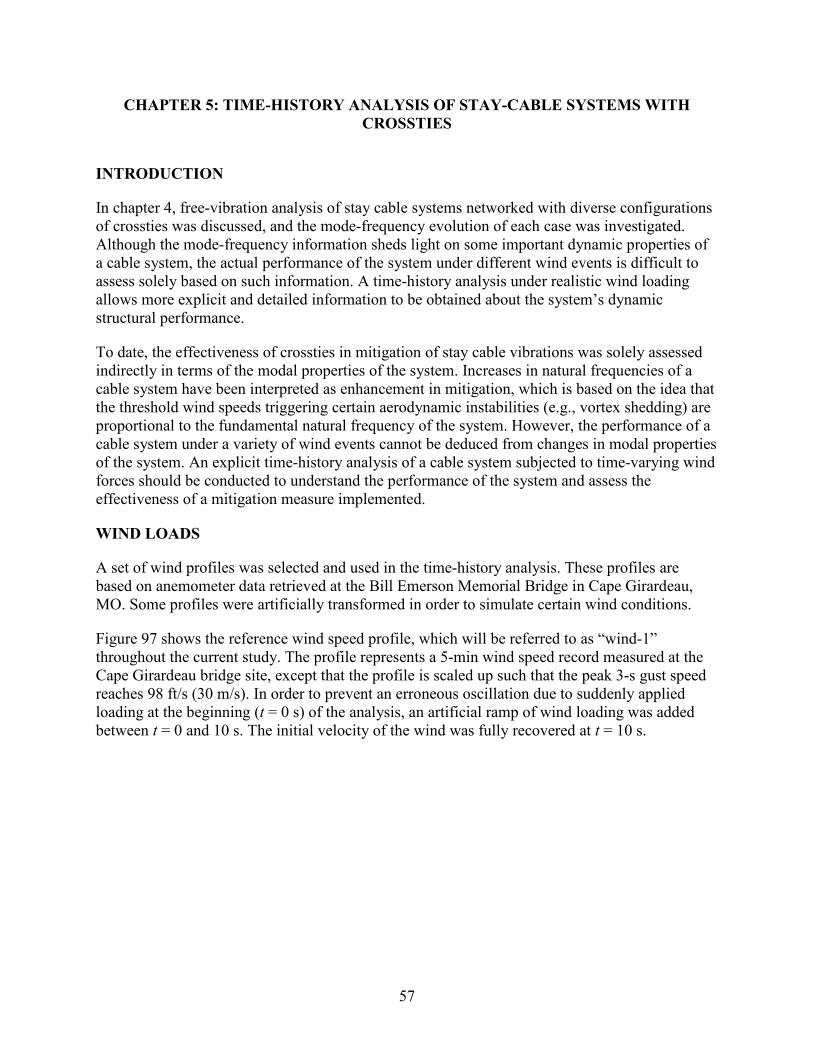
CHAPTER 5: TIME-HISTORY ANALYSIS OF STAY-CABLE SYSTEMS WITH CROSSTIES

INTRODUCTION

In chapter 4, free-vibration analysis of stay cable systems networked with diverse configurations of crossties was discussed, and the mode-frequency evolution of each case was investigated. Although the mode-frequency information sheds light on some important dynamic properties of a cable system, the actual performance of the system under different wind events is difficult to assess solely based on such information. A time-history analysis under realistic wind loading allows more explicit and detailed information to be obtained about the system’s dynamic structural performance.

To date, the effectiveness of crossties in mitigation of stay cable vibrations was solely assessed indirectly in terms of the modal properties of the system. Increases in natural frequencies of a cable system have been interpreted as enhancement in mitigation, which is based on the idea that the threshold wind speeds triggering certain aerodynamic instabilities (e.g., vortex shedding) are proportional to the fundamental natural frequency of the system. However, the performance of a cable system under a variety of wind events cannot be deduced from changes in modal properties of the system. An explicit time-history analysis of a cable system subjected to time-varying wind forces should be conducted to understand the performance of the system and assess the effectiveness of a mitigation measure implemented.

WIND LOADS

A set of wind profiles was selected and used in the time-history analysis. These profiles are based on anemometer data retrieved at the Bill Emerson Memorial Bridge in Cape Girardeau, MO. Some profiles were artificially transformed in order to simulate certain wind conditions.

Figure 97 shows the reference wind speed profile, which will be referred to as “wind-1” throughout the current study. The profile represents a 5-min wind speed record measured at the Cape Girardeau bridge site, except that the profile is scaled up such that the peak 3-s gust speed reaches 98 ft/s (30 m/s). In order to prevent an erroneous oscillation due to suddenly applied loading at the beginning (t = 0 s) of the analysis, an artificial ramp of wind loading was added between t = 0 and 10 s. The initial velocity of the wind was fully recovered at t = 10 s.

57

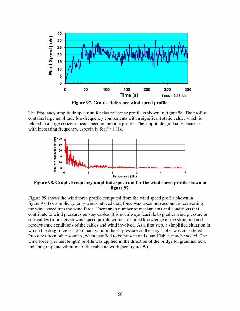
Figure 97. Graph. Reference wind speed profile.

The frequency-amplitude spectrum for this reference profile is shown in figure 98. The profile contains large amplitude low-frequency components with a significant static value, which is related to a large nonzero mean speed in the time profile. The amplitude gradually decreases with increasing frequency, especially for f > 1 Hz.

Figure 98. Graph. Frequency-amplitude spectrum for the wind speed profile shown in

figure 97.

Figure 99 shows the wind force profile computed from the wind speed profile shown in figure 97. For simplicity, only wind-induced drag force was taken into account in converting the wind speed into the wind force. There are a number of mechanisms and conditions that contribute to wind pressures on stay cables. It is not always feasible to predict wind pressure on stay cables from a given wind speed profile without detailed knowledge of the structural and aerodynamic conditions of the cables and wind involved. As a first step, a simplified situation in which the drag force is a dominant wind-induced pressure on the stay cables was considered. Pressures from other sources, when justified to be present and quantifiable, may be added. The wind force (per unit length) profile was applied in the direction of the bridge longitudinal axis, inducing in-plane vibration of the cable network (see figure 99).

58

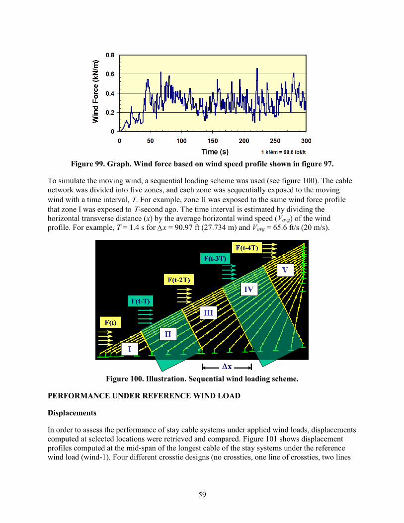
Figure 99. Graph. Wind force based on wind speed profile shown in figure 97.

To simulate the moving wind, a sequential loading scheme was used (see figure 100). The cable network was divided into five zones, and each zone was sequentially exposed to the moving wind with a time interval, Τ. For example, zone II was exposed to the same wind force profile that zone I was exposed to Τ-second ago. The time interval is estimated by dividing the horizontal transverse distance (x) by the average horizontal wind speed (Vavg) of the wind profile. For example, T = 1.4 s for x = 90.97 ft (27.734 m) and Vavg = 65.6 ft/s (20 m/s).

Figure 100. Illustration. Sequential wind loading scheme.

PERFORMANCE UNDER REFERENCE WIND LOAD

Displacements

In order to assess the performance of stay cable systems under applied wind loads, displacements computed at selected locations were retrieved and compared. Figure 101 shows displacement profiles computed at the mid-span of the longest cable of the stay systems under the reference wind load (wind-1). Four different crosstie designs (no crossties, one line of crossties, two lines

∆

59

of crossties, and four lines of crossties) were considered. The displacements, Ux, are the horizontal components parallel to the bridge axis.

Figure 101. Graph. Displacement computed at the mid-span of cable 1 with no crossties,

one line of crossties, two lines of crossties, and four lines of crossties.

Among the four cases considered, the system with two lines of crossties produced the least displacement. However, the behavior may depend on the location where displacements were retrieved. Figure 102 through figure 104 show the displacement profiles computed at other locations within the system: at a quarter-span of the longest cable (figure 102), at the network center (figure 103), and at the mid-span of the shortest cable (figure 104). At a quarter-span, the system with four lines of crossties had the least displacement, while at the network center, the system with two lines of crossties had the least displacement. It is difficult to judge the mitigation effectiveness of a crosstied cable network simply by looking at displacements at some selected locations. Instead, mechanical energies of a system can be used as a global indicator of the performance, as will be discussed later.

60

Figure 102. Graph. Displacement computed at the quarter-span of cable 1 with no

crossties, one line of crossties, two lines of crossties, and four lines of crossties.

Figure 103. Graph. Displacement computed at the center of the network with no crossties,


61

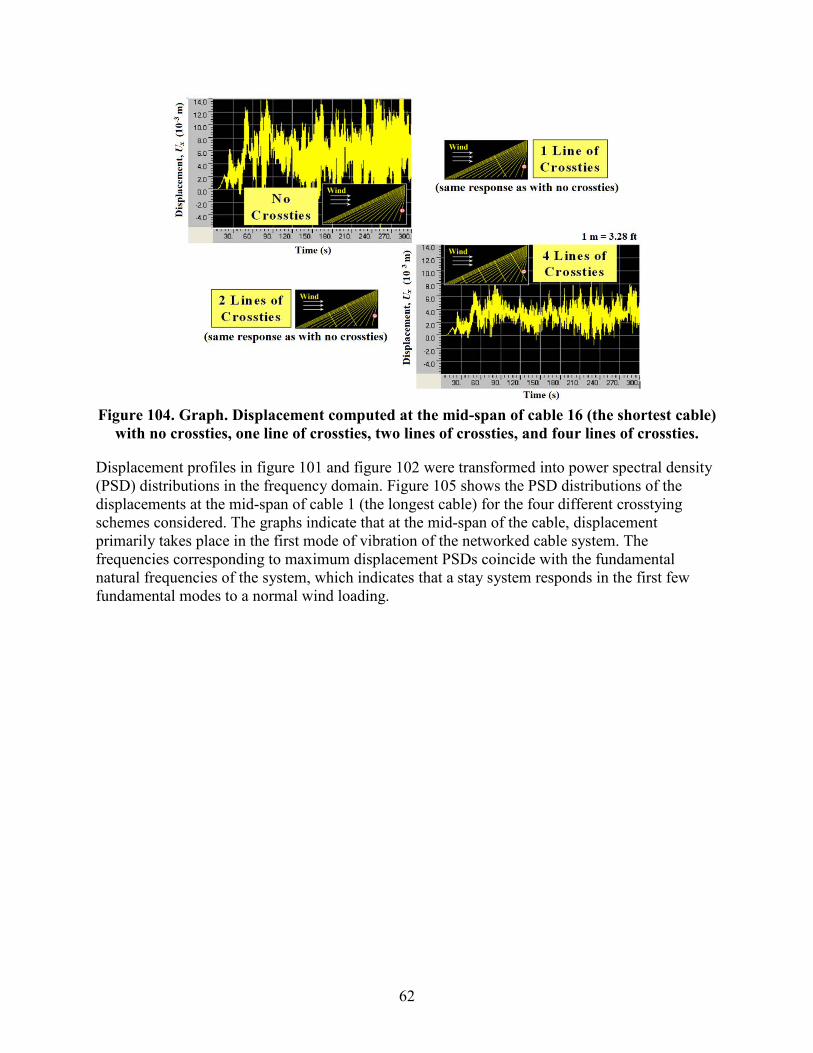
Figure 104. Graph. Displacement computed at the mid-span of cable 16 (the shortest cable)

with no crossties, one line of crossties, two lines of crossties, and four lines of crossties.

Displacement profiles in figure 101 and figure 102 were transformed into power spectral density (PSD) distributions in the frequency domain. Figure 105 shows the PSD distributions of the displacements at the mid-span of cable 1 (the longest cable) for the four different crosstying schemes considered. The graphs indicate that at the mid-span of the cable, displacement primarily takes place in the first mode of vibration of the networked cable system. The frequencies corresponding to maximum displacement PSDs coincide with the fundamental natural frequencies of the system, which indicates that a stay system responds in the first few fundamental modes to a normal wind loading.

62

Figure 105. Graph. PSD of the displacement at the mid-span of cable 1 with no crossties,


The fundamental (i.e., first mode) natural frequency of the system with no crossties, one line of crossties, two lines of crossties, and four lines of crossties are 0.56, 0.87, 1.18, and 1.38 Hz, respectively. For the system without crossties, the first-mode frequency of the system coincides with the first mode frequency of the longest cable. The system with two lines of crossties exhibited small displacement (figure 101), and the corresponding PSD was negligibly small compared to other three cases considered (figure 105). Note the large static value (f = 0 Hz) registered for the case of no crossties and very limited static component for the system with four lines of crossties.

Figure 106 show PSD distributions of the displacements at the quarter-span of cable 1 for the same four crosstying schemes considered. Again, the largest PSD occurred at the first mode of each system; however, additional peaks appeared at the second and third mode frequencies. A large-value PSD was registered at the fundamental mode for the two-line system.

63

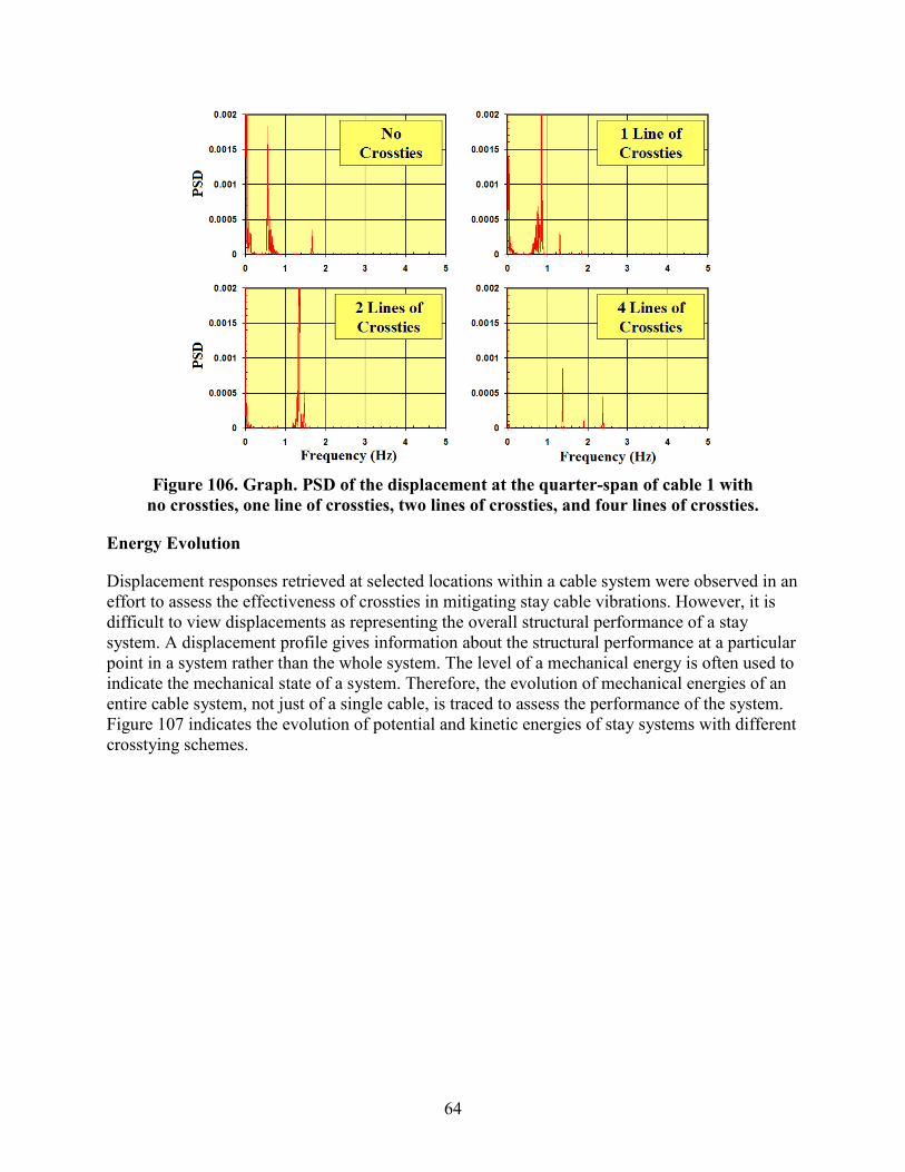
Figure 106. Graph. PSD of the displacement at the quarter-span of cable 1 with

no crossties, one line of crossties, two lines of crossties, and four lines of crossties.

Energy Evolution

Displacement responses retrieved at selected locations within a cable system were observed in an effort to assess the effectiveness of crossties in mitigating stay cable vibrations. However, it is difficult to view displacements as representing the overall structural performance of a stay system. A displacement profile gives information about the structural performance at a particular point in a system rather than the whole system. The level of a mechanical energy is often used to indicate the mechanical state of a system. Therefore, the evolution of mechanical energies of an entire cable system, not just of a single cable, is traced to assess the performance of the system. Figure 107 indicates the evolution of potential and kinetic energies of stay systems with different crosstying schemes.

64

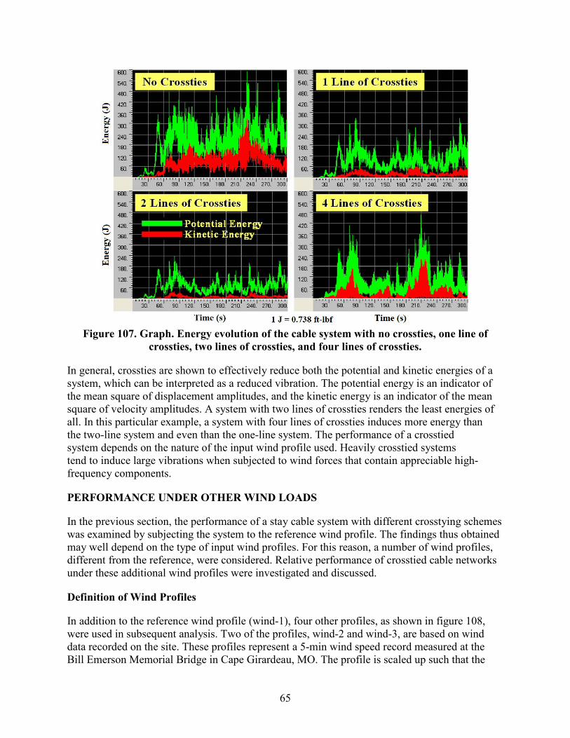
Figure 107. Graph. Energy evolution of the cable system with no crossties, one line of

crossties, two lines of crossties, and four lines of crossties.

In general, crossties are shown to effectively reduce both the potential and kinetic energies of a system, which can be interpreted as a reduced vibration. The potential energy is an indicator of the mean square of displacement amplitudes, and the kinetic energy is an indicator of the mean square of velocity amplitudes. A system with two lines of crossties renders the least energies of all. In this particular example, a system with four lines of crossties induces more energy than the two-line system and even than the one-line system. The performance of a crosstied system depends on the nature of the input wind profile used. Heavily crosstied systems tend to induce large vibrations when subjected to wind forces that contain appreciable high-frequency components.

PERFORMANCE UNDER OTHER WIND LOADS

In the previous section, the performance of a stay cable system with different crosstying schemes was examined by subjecting the system to the reference wind profile. The findings thus obtained may well depend on the type of input wind profiles. For this reason, a number of wind profiles, different from the reference, were considered. Relative performance of crosstied cable networks under these additional wind profiles were investigated and discussed.

Definition of Wind Profiles

In addition to the reference wind profile (wind-1), four other profiles, as shown in figure 108, were used in subsequent analysis. Two of the profiles, wind-2 and wind-3, are based on wind data recorded on the site. These profiles represent a 5-min wind speed record measured at the Bill Emerson Memorial Bridge in Cape Girardeau, MO. The profile is scaled up such that the

65

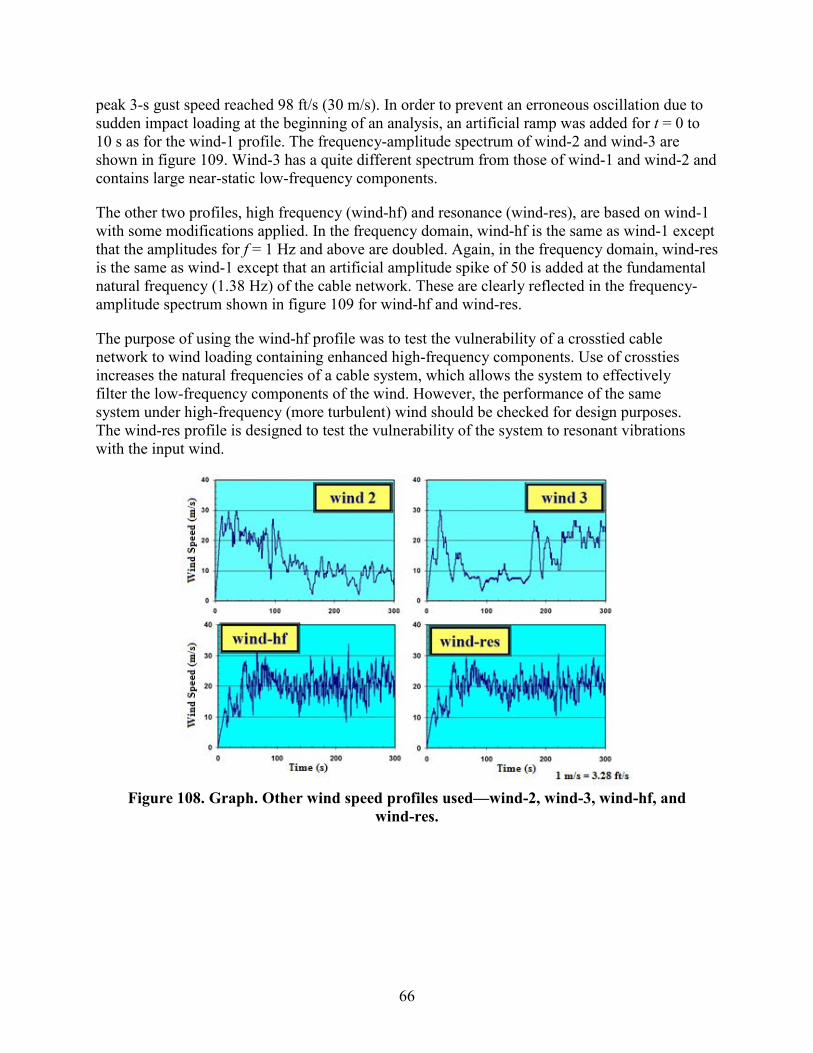
peak 3-s gust speed reached 98 ft/s (30 m/s). In order to prevent an erroneous oscillation due to sudden impact loading at the beginning of an analysis, an artificial ramp was added for t = 0 to 10 s as for the wind-1 profile. The frequency-amplitude spectrum of wind-2 and wind-3 are shown in figure 109. Wind-3 has a quite different spectrum from those of wind-1 and wind-2 and contains large near-static low-frequency components.

The other two profiles, high frequency (wind-hf) and resonance (wind-res), are based on wind-1 with some modifications applied. In the frequency domain, wind-hf is the same as wind-1 except that the amplitudes for f = 1 Hz and above are doubled. Again, in the frequency domain, wind-res is the same as wind-1 except that an artificial amplitude spike of 50 is added at the fundamental natural frequency (1.38 Hz) of the cable network. These are clearly reflected in the frequency-amplitude spectrum shown in figure 109 for wind-hf and wind-res.

The purpose of using the wind-hf profile was to test the vulnerability of a crosstied cable network to wind loading containing enhanced high-frequency components. Use of crossties increases the natural frequencies of a cable system, which allows the system to effectively filter the low-frequency components of the wind. However, the performance of the same system under high-frequency (more turbulent) wind should be checked for design purposes. The wind-res profile is designed to test the vulnerability of the system to resonant vibrations with the input wind.

Figure 108. Graph. Other wind speed profiles used—wind-2, wind-3, wind-hf, and

wind-res.

66

Figure 109. Graph. Frequency-amplitude spectra of the wind profiles used—wind-2,

wind-3, wind-hf, and wind-res.

Response to Wind-2

Displacement time-histories at the mid-span of cable 1 when the cable system was subjected to wind-2 are presented in figure 110 for the four different crosstying schemes. It can be seen that the use of crossties greatly reduced cable vibrations. Energy evolution under wind-2 is shown in figure 111. Both displacement and energy evolution data indicate that a system with two lines of crossties best mitigates cable vibrations induced by wind-2. The four-line system appears to be effective in controlling static displacements but not quite in controlling vibration amplitudes.

67

Figure 110. Graph. Displacement computed at the mid-span of cable 1 when the cable

network is subjected to wind-2 with no crossties, one line of crossties, two lines of crossties, and four lines of crossties.

Figure 111. Graph. Energy evolution of the cable system subjected to wind-2 with no crossties, one line of crossties, two lines of crossties, and four lines of crossties.

Response to Wind-3

Responses of the cable systems to wind-3 are presented in figure 112 for mid-span displacements and in figure 113 for energy evolutions. Both sets of figures indicate that the influence of

68

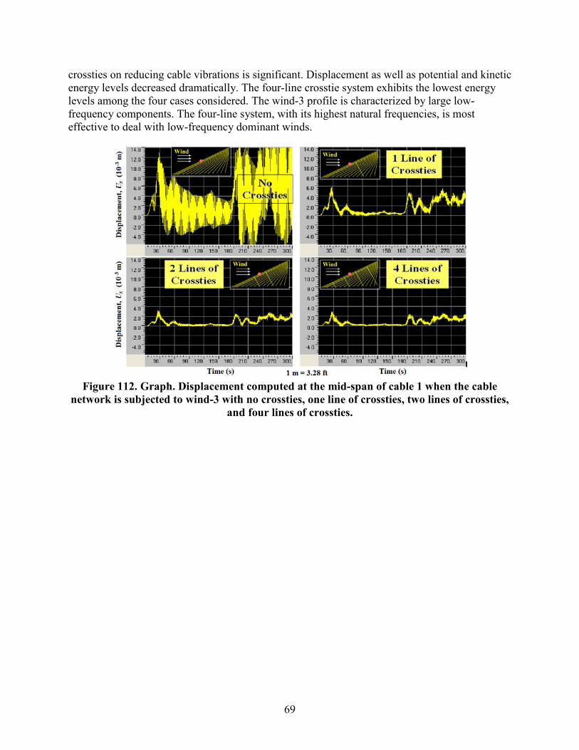
crossties on reducing cable vibrations is significant. Displacement as well as potential and kinetic energy levels decreased dramatically. The four-line crosstie system exhibits the lowest energy levels among the four cases considered. The wind-3 profile is characterized by large low-frequency components. The four-line system, with its highest natural frequencies, is most effective to deal with low-frequency dominant winds.


network is subjected to wind-3 with no crossties, one line of crossties, two lines of crossties, and four lines of crossties.

69

Figure 113. Graph. Energy evolution of the cable system subjected to wind-3 with no crossties, one line of crossties, two lines of crossties, and four lines of crossties.

Response to Wind-hf

Displacements under wind-hf are shown in figure 114, and energy evolutions under wind-hf are shown in figure 115. It is clear that the mitigation effectiveness of crossties significantly decreased when the system was subjected to high-frequency enhanced wind. Benefits of the use of crossties appear to be proportional to the quantity of crossties to a certain degree. However, further increases in crosstie quantity resulted in increased magnitudes of cable vibration. Under an artificial profile, wind-hf, the performance of a cable system gradually improved up until the two-line system. However, for the four-line system, the performance became worse. The four-line system clearly shows its response sensitivity to high-frequency wind components.

70


network is subjected to wind-hf with no crossties, one line of crossties, two lines of crossties, and four lines of crossties.

Figure 115. Graph. Energy evolution of the cable system subjected to wind-hf with no crossties, one line of crossties, two lines of crossties, and four lines of crossties.

In general, the results suggest that the use of crossties helps mitigate wind-induced stay cable vibrations. However, as the quantity of crossties increases beyond a certain threshold, the system becomes more vulnerable to high-frequency components of winds. Therefore, the performance of a crosstied network is sensitive to the frequency content of wind loading. Crossties are

71

particularly effective in reducing low-frequency components of cable vibrations. Performance of a crosstied network is not necessarily proportional to its quantity (or number of lines) of crossties. An excessive provision of crossties may result in an adverse effect under highly turbulent winds (if present).

Response to Wind-res

The displacement of a cable system with four lines of crossties subjected to wind-1 and wind-res at the mid-span of cable 1 are shown in figure 116. Figure 117 shows the PSD distributions of the displacement profiles shown in figure 116. A noticeable peak is present at the resonant frequency (f = 1.38 Hz) of the system when the system is subjected to wind-res. Energy evolution, which is presented in figure 118, confirms the fact that a system responds sensitively to a wind load containing a finite amplitude at the system’s resonant frequency.

Figure 116. Graph. Displacement at the mid-span of cable 1 when the cable network with

four lines of crossties is subjected to wind-1 (left) and wind-res (right).

Figure 117. Graph. PSD of the displacement at the mid-span of cable 1 when the cable network with four lines of crossties is subjected to wind-1 (left) and wind-res (right).

72

Figure 118. Graph. Energy evolution of the cable network with four lines of crossties

subjected to wind-1 (left) and wind-res (right).

It can be seen that a slight magnification of the wind component at the resonant frequency of the input wind load results in a dramatically magnified response of the system, which indicates the vulnerability of a cable system to resonant wind loading. The system quickly builds up a resonant vibration with its limited inherent damping. The addition of dampers may effectively lower the potential of such occurrence.

AXIAL AND SHEAR FORCES

Peak axial force distribution in cables and crossties is presented in figure 119. Particular attention was given to the compressive forces in the crossties to see if they were within the pre-tension levels. The axial forces shown do not include pre-tensions applied to the cables and crossties during construction. The maximum peak compressive force in the crossties was 5.2 kip (23 kN), which is within the applied pre-tension level of 7.9 kip (35 kN). This insures that the crossties remain taut throughout the event. The pre-tension level required to prevent the slack of the crossties depends on the severity of the design wind event.

Figure 119. Image. Peak axial force distribution under wind-1.

Peak shear force distribution in cables and crossties is shown in figure 120. Since cables and crossties are modeled as beams with transverse stiffnesses, they carry shear forces. Largest shear

73

forces are experienced at the cable supports and at the cable/crosstie junctions, which must be taken into account in design of a crosstying system.

Figure 120. Image. Peak shear force distribution under wind-1.

74

CHAPTER 6: TIME-HISTORY ANALYSIS OF STAY CABLES WITH EXTERNAL DAMPERS

INTRODUCTION

Dampers are frequently used to suppress excessive vibration of stay cables which have limited intrinsic damping. These dampers, due to practical limitations of installation, are usually attached to the stay cables near the anchorages. Although theories behind the observed behavior of stays with attached dampers are not completely developed, dampers have been widely used, and their effectiveness has been demonstrated by many examples. Application of dampers for cable vibration mitigation is anticipated to be more widespread, and the need for improved understanding of the resulting dynamic system is increasing. The effectiveness of different strategies involving external dampers and crossties for mitigation of stay cable vibrations is investigated via finite element simulations.

CONFIGURATION AND DAMPER COEFFICIENT

Figure 121 shows a single stay with a viscous damper attached near the anchorage. The distance of the damper from the deck anchorage is 2 percent of the chord length of the cable (d = 0.02 L). The stay simulates Cable SWC-01 of the Cape Girardeau Bridge, whose properties are presented in table 2 and table 3 (see cable 1). A sequential wind loading on the cable is shown in figure 122, in which F(t) denotes the horizontal wind force history shown in figure 99.

Figure 121. Image. Stay cable with a viscous damper attached to it.

Damper connectd to the deck at d = 0.02L

L

d Damper connectd to the deck at d = 0.02L

L

d

75

Figure 122. Image. Sequential wind loading on the cable.

The optimal damping coefficient (Copt) for the cable is determined from the universal damping curve shown in figure 123. This asymptotic analytical curve proposed by Krenk is valid when d/L, the relative damper distance from the support, is very small.(15)

Figure 123. Graph. Universal damping curve.

The curve relates the normalized damping ratio i/(d/L) to the normalized damping coefficient ( ) defined as follows:

Figure 124. Equation. Normalized damping coefficient.

Where:

C = Damper coefficient. m = Cable mass per unit length.

I

IV

II

III

V

F(t)

F(t-T)

F(t-2T)

F(t-3T)

F(t-4T)

0

0.1

0.2

0.3

0.4

0.5

0.6

0 0.1 0.2 0.3 0.4 0.5 0.6 0.7 0.8 0.9 1

( )Ld

iζ

κ

ζ κ

76

ω 1 = First mode natural frequency. ζ i = Damping ratio of the ith mode of vibration. i = Mode number.

At optimal damping, the normalized damping ratio reaches 0.5 and approaches 0.1, from which C-values are determined for different modes. The achievable modal damping ratios are limited by this relationship. For example, for d/L of 2 percent, the achievable maximum damping ratio for the first mode is 1 percent.

RESPONSE TO REFERENCE WIND LOAD

Figure 125 and figure 126 show the horizontal components of the displacement histories computed at the mid- and quarter-span of the stay without and with a damper, respectively. It can be seen that the use of a damper reduces the vibration amplitudes of the stay. Figure 127 shows the energy evolution of the stay without and with a damper, respectively. Both the potential and kinetic energies are reduced due to the incorporation of a damper; however, the reduction of kinetic energy is more pronounced than that of potential energy. When damper is not used, the energy of the cable is dissipated entirely by intrinsic modal damping. A uniform modal damping of 0.3 percent is assumed. When a damper is used, the majority of the energy is dissipated via the damper, and only a small fraction of the energy is dissipated via intrinsic damping of the cable.

Figure 125. Graph. Displacement computed at mid-span of the cable without damper (left)

and with damper (right).

Figure 126. Graph. Displacement computed at quarter-span of the cable without damper

(left) and with damper (right).

κ

77

Figure 127. Graph. Energy evolution of the cable without damper (left) and with damper

(right).

Figure 128 and figure 129 show the PSD distributions for the displacement profiles computed at the mid- and quarter-span of the stay, respectively. Without damper, vibration took place primarily in the first and third modes, whereas when a damper was installed, the vibration was mostly in the first mode, and only a small trace in the third mode was observed. According to the theory, the use of a damper shifts the natural vibration frequencies of the stay; however, in this particular example, the amount of shift appears to be very limited.

Figure 128. Graph. PSD for displacement at mid-span of the cable without damper (left)

and with damper (right).

78

Figure 129. Graph. PSD for displacement at quarter-span of the cable without damper

(left) and with damper (right).

Figure 130 shows the energy evolution of a single cable without and with a damper subjected to wind-hf. The effectiveness of the use of a damper is more pronounced when a stay is subjected to a wind event that contains enriched high-frequency components. In other words, dampers are more efficient in mitigating stay vibrations containing appreciable high-frequency components. The major portion of the vibration energy is dissipated via the damper. It is to be noted that dampers are effective in mitigating transverse and in-plane vibrations when separate dampers are installed in the respective directions of motion.

Figure 130. Graph. Energy evolution of the cable under wind-hf without damper (left) and

with damper (right).

INFLUENCE OF DAMPER PARAMETERS

The efficiency of a damper depends primarily on its damping coefficient and its location on the stay, among other factors. In order to test the influence of damping coefficient (or damper coefficient), four different levels of damping were considered: C = 0 (no damper), C = Copt, C = 0.1 Copt, and C = 10 Copt. Results are shown in figure 131, which highlights the evolution of the potential and kinetic energy of a cable/damper system subjected to wind-1. Also shown are energies dissipated through intrinsic modal damping and through the damper.

79

Figure 131. Graph. Energy evolution of the cable when different levels of damper

coefficient are used—(a) C = 0 (no damper), (b) C = Copt, (c) C = 0.1 Copt, and (d) C = 10 Copt.

As can be expected, the cable performed best when the damper had its optimal coefficient, C = Copt. Energy levels, especially kinetic energy, are lowest when the optimal value is used. It can be seen that with the optimal damper coefficient (see graph b in figure 131), the amount of energy dissipated through the damper is greatest, and the demand of energy dissipation through the cable’s intrinsic modal damping is minimal. Dissipation by modal damping is proportional to kinetic energy due to their dependence on velocity. Therefore, less dissipation by modal damping signifies a lower level of kinetic energy, meaning lesser cable vibrations.

To test the influence of damper location, four different cases were considered. Figure 132 shows results for C = 0 (no damper), d/L = 0.02, d/L = 0.05, and d/L = 0.10, where d is the offset distance of the damper from anchorage, and L is the chord length of the stay cable. The case of d/L = 0.10 gives the largest energy dissipation through the damper, and the achieved kinetic energy level is lowest among the four cases considered, signifying its being the most effective in vibration mitigation. However, due to practical limitations associated with installation, dampers are usually attached to stays near the anchorages.

80

Figure 132. Graph. Energy evolution of the cable when different damper locations are

used—(a) C = 0 (no damper), (b) d/L = 0.02, (c) d/L = 0.05, and (d) d/L = 0.10.

81

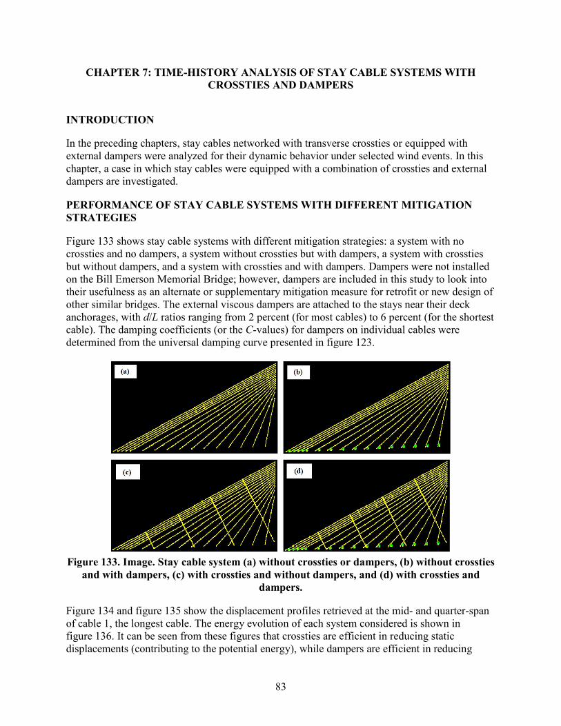
CHAPTER 7: TIME-HISTORY ANALYSIS OF STAY CABLE SYSTEMS WITH CROSSTIES AND DAMPERS

INTRODUCTION

In the preceding chapters, stay cables networked with transverse crossties or equipped with external dampers were analyzed for their dynamic behavior under selected wind events. In this chapter, a case in which stay cables were equipped with a combination of crossties and external dampers are investigated.

PERFORMANCE OF STAY CABLE SYSTEMS WITH DIFFERENT MITIGATION STRATEGIES

Figure 133 shows stay cable systems with different mitigation strategies: a system with no crossties and no dampers, a system without crossties but with dampers, a system with crossties but without dampers, and a system with crossties and with dampers. Dampers were not installed on the Bill Emerson Memorial Bridge; however, dampers are included in this study to look into their usefulness as an alternate or supplementary mitigation measure for retrofit or new design of other similar bridges. The external viscous dampers are attached to the stays near their deck anchorages, with d/L ratios ranging from 2 percent (for most cables) to 6 percent (for the shortest cable). The damping coefficients (or the C-values) for dampers on individual cables were determined from the universal damping curve presented in figure 123.

Figure 133. Image. Stay cable system (a) without crossties or dampers, (b) without crossties

and with dampers, (c) with crossties and without dampers, and (d) with crossties and dampers.

Figure 134 and figure 135 show the displacement profiles retrieved at the mid- and quarter-span of cable 1, the longest cable. The energy evolution of each system considered is shown in figure 136. It can be seen from these figures that crossties are efficient in reducing static displacements (contributing to the potential energy), while dampers are efficient in reducing

83

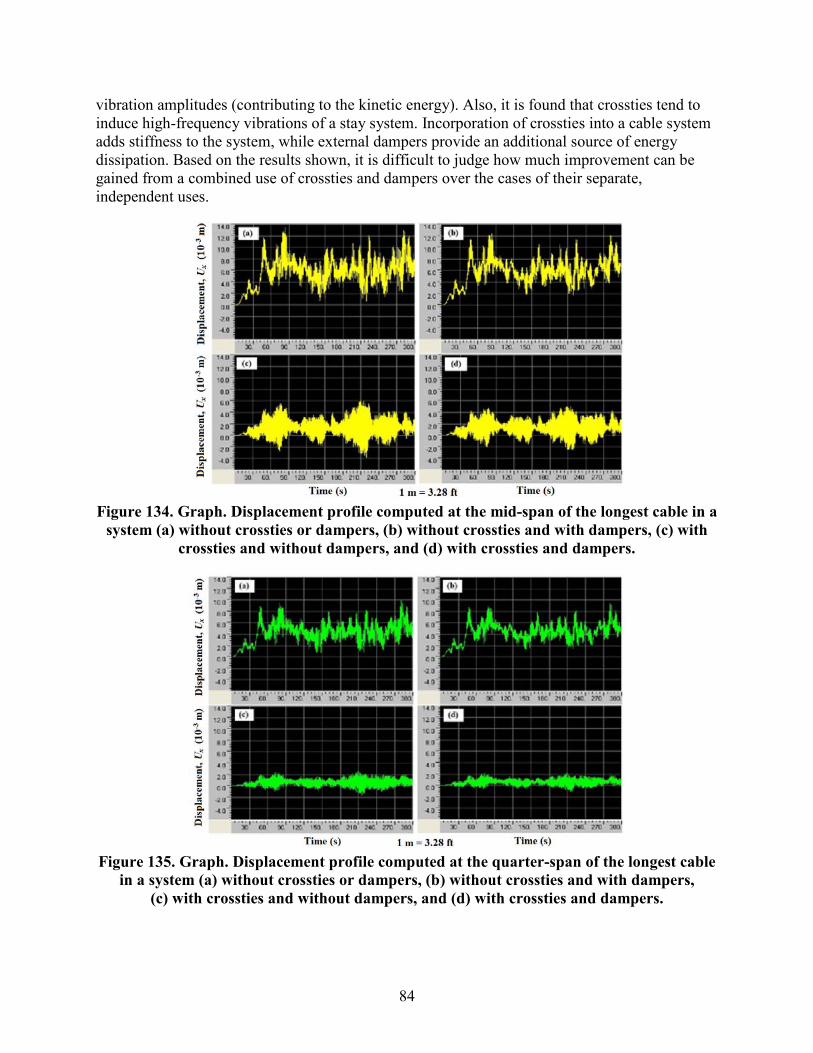
vibration amplitudes (contributing to the kinetic energy). Also, it is found that crossties tend to induce high-frequency vibrations of a stay system. Incorporation of crossties into a cable system adds stiffness to the system, while external dampers provide an additional source of energy dissipation. Based on the results shown, it is difficult to judge how much improvement can be gained from a combined use of crossties and dampers over the cases of their separate, independent uses.

Figure 134. Graph. Displacement profile computed at the mid-span of the longest cable in a

system (a) without crossties or dampers, (b) without crossties and with dampers, (c) with crossties and without dampers, and (d) with crossties and dampers.

Figure 135. Graph. Displacement profile computed at the quarter-span of the longest cable

in a system (a) without crossties or dampers, (b) without crossties and with dampers, (c) with crossties and without dampers, and (d) with crossties and dampers.

84

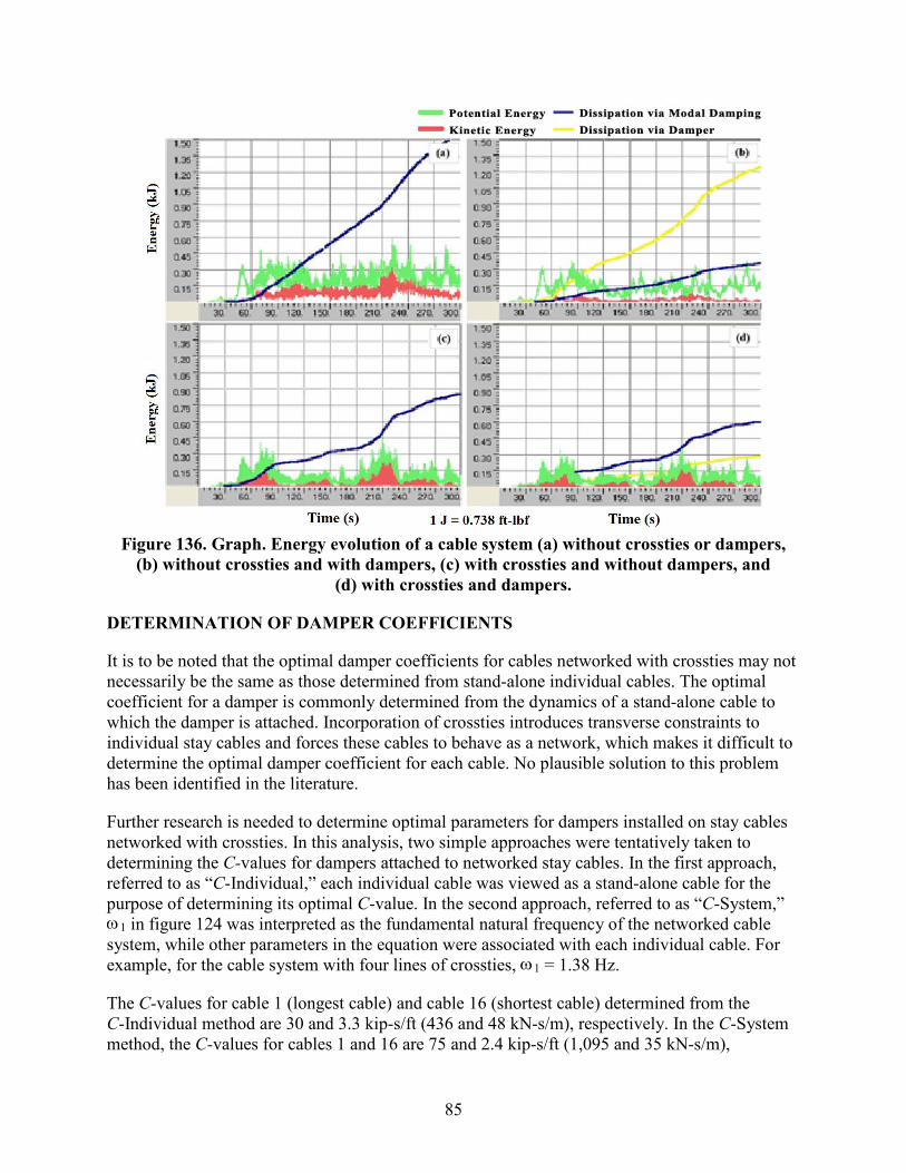
Figure 136. Graph. Energy evolution of a cable system (a) without crossties or dampers,

(b) without crossties and with dampers, (c) with crossties and without dampers, and (d) with crossties and dampers.

DETERMINATION OF DAMPER COEFFICIENTS

It is to be noted that the optimal damper coefficients for cables networked with crossties may not necessarily be the same as those determined from stand-alone individual cables. The optimal coefficient for a damper is commonly determined from the dynamics of a stand-alone cable to which the damper is attached. Incorporation of crossties introduces transverse constraints to individual stay cables and forces these cables to behave as a network, which makes it difficult to determine the optimal damper coefficient for each cable. No plausible solution to this problem has been identified in the literature.

Further research is needed to determine optimal parameters for dampers installed on stay cables networked with crossties. In this analysis, two simple approaches were tentatively taken to determining the C-values for dampers attached to networked stay cables. In the first approach, referred to as “C-Individual,” each individual cable was viewed as a stand-alone cable for the purpose of determining its optimal C-value. In the second approach, referred to as “C-System,”

1 in figure 124 was interpreted as the fundamental natural frequency of the networked cable system, while other parameters in the equation were associated with each individual cable. For example, for the cable system with four lines of crossties, 1 = 1.38 Hz.

The C-values for cable 1 (longest cable) and cable 16 (shortest cable) determined from the C-Individual method are 30 and 3.3 kip-s/ft (436 and 48 kN-s/m), respectively. In the C-System method, the C-values for cables 1 and 16 are 75 and 2.4 kip-s/ft (1,095 and 35 kN-s/m),

ω

ω

85

respectively. Figure 137 and figure 138 compare the results from the displacement and energy evolution approaches, respectively. The difference in results from the two methods is negligibly small, which suggests insensitivity of the system behavior to small variations of C-values.

Figure 137. Graph. Comparison of displacements at mid-span of the longest cable when damper coefficients are used based on individual cables’ natural frequencies (left) and

when damper coefficients are used based on a cable system’s natural frequencies (right).

Figure 138. Graph. Comparison of energy evolution of the system when damper

coefficients are used based on individual cables’ natural frequencies (left) and when damper coefficients are used based on a cable system’s natural frequencies (right).

In order to check the system performance under larger variations of C-values, four different cases were considered: C = Copt, C = 5 Copt, C = 10 Copt, and C = 100 Copt. Figure 139 compares the energy evolution of the cable system when these four different C-values are used. Among the four cases tested, C = 5 Copt gives the best result with largest energy dissipation via dampers (thus resulting in smallest dissipation demand via cable’s intrinsic modal damping). As the C-value further increases, the vibration of the cable system increases. It is to be noted that Copt denotes the optimal damper coefficient for a damper attached to a stand-alone stay cable, not a networked cable. This experiment suggests that when dampers are attached to stays networked with crossties, larger dampers are required than when dampers are attached to stays not networked with crossties.

86

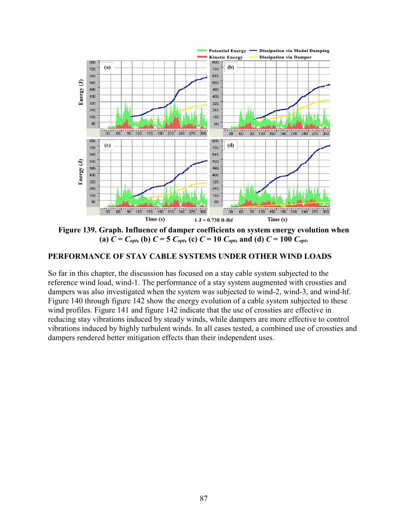
Figure 139. Graph. Influence of damper coefficients on system energy evolution when

(a) C = Copt, (b) C = 5 Copt, (c) C = 10 Copt, and (d) C = 100 Copt.

PERFORMANCE OF STAY CABLE SYSTEMS UNDER OTHER WIND LOADS

So far in this chapter, the discussion has focused on a stay cable system subjected to the reference wind load, wind-1. The performance of a stay system augmented with crossties and dampers was also investigated when the system was subjected to wind-2, wind-3, and wind-hf. Figure 140 through figure 142 show the energy evolution of a cable system subjected to these wind profiles. Figure 141 and figure 142 indicate that the use of crossties are effective in reducing stay vibrations induced by steady winds, while dampers are more effective to control vibrations induced by highly turbulent winds. In all cases tested, a combined use of crossties and dampers rendered better mitigation effects than their independent uses.

87

Figure 140. Graph. Energy evolution of the cable system under wind-2 (a) without crossties

or dampers, (b) without crossties and with dampers, (c) with crossties and without dampers, and (d) with crossties and dampers.

Figure 141. Graph. Energy evolution of the cable system under wind-3 (a) without crossties

or dampers, (b) without crossties and with dampers, (c) with crossties and without dampers, and (d) with crossties and dampers.

88

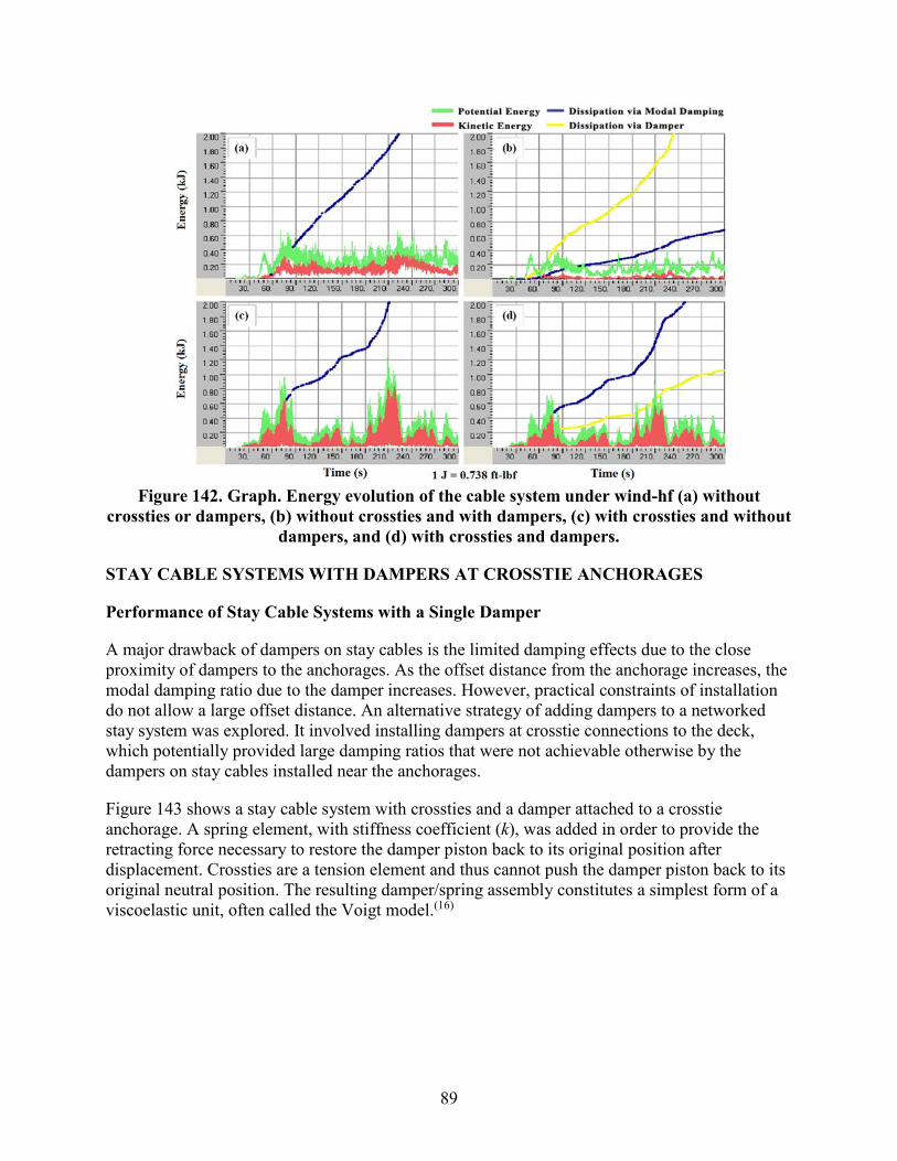
Figure 142. Graph. Energy evolution of the cable system under wind-hf (a) without

crossties or dampers, (b) without crossties and with dampers, (c) with crossties and without dampers, and (d) with crossties and dampers.

STAY CABLE SYSTEMS WITH DAMPERS AT CROSSTIE ANCHORAGES

Performance of Stay Cable Systems with a Single Damper

A major drawback of dampers on stay cables is the limited damping effects due to the close proximity of dampers to the anchorages. As the offset distance from the anchorage increases, the modal damping ratio due to the damper increases. However, practical constraints of installation do not allow a large offset distance. An alternative strategy of adding dampers to a networked stay system was explored. It involved installing dampers at crosstie connections to the deck, which potentially provided large damping ratios that were not achievable otherwise by the dampers on stay cables installed near the anchorages.

Figure 143 shows a stay cable system with crossties and a damper attached to a crosstie anchorage. A spring element, with stiffness coefficient (k), was added in order to provide the retracting force necessary to restore the damper piston back to its original position after displacement. Crossties are a tension element and thus cannot push the damper piston back to its original neutral position. The resulting damper/spring assembly constitutes a simplest form of a viscoelastic unit, often called the Voigt model.(16)

89

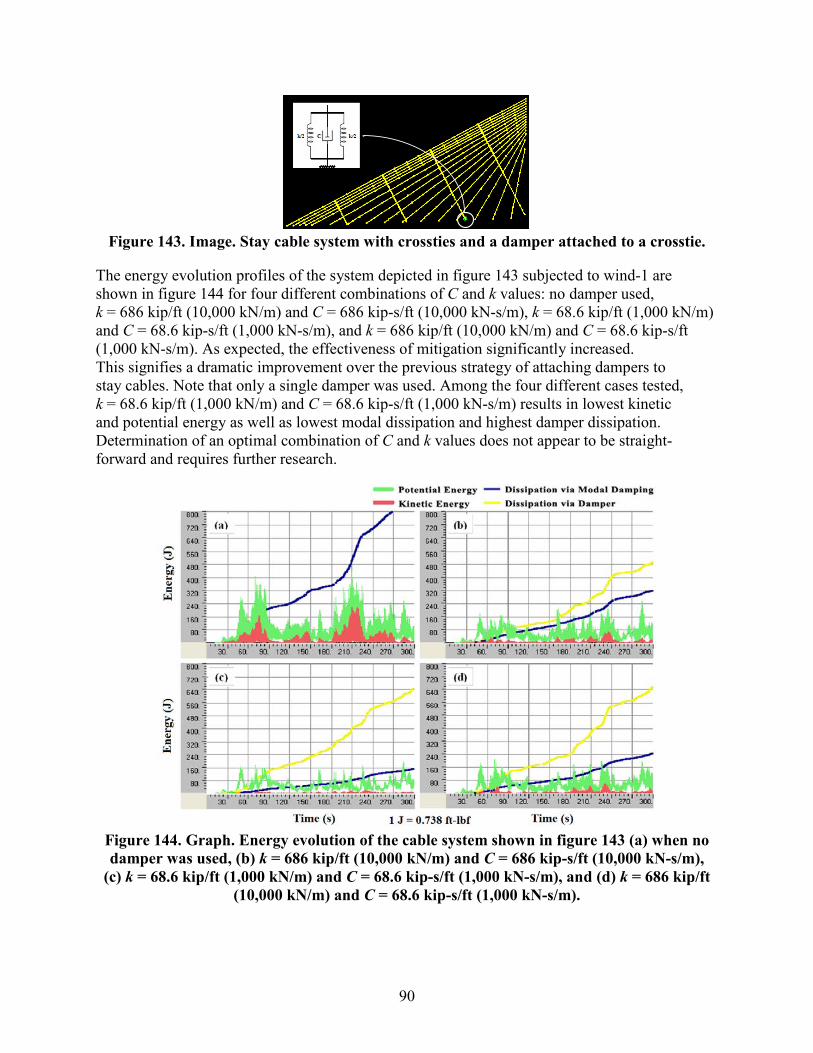
Figure 143. Image. Stay cable system with crossties and a damper attached to a crosstie.

The energy evolution profiles of the system depicted in figure 143 subjected to wind-1 are shown in figure 144 for four different combinations of C and k values: no damper used, k = 686 kip/ft (10,000 kN/m) and C = 686 kip-s/ft (10,000 kN-s/m), k = 68.6 kip/ft (1,000 kN/m) and C = 68.6 kip-s/ft (1,000 kN-s/m), and k = 686 kip/ft (10,000 kN/m) and C = 68.6 kip-s/ft (1,000 kN-s/m). As expected, the effectiveness of mitigation significantly increased. This signifies a dramatic improvement over the previous strategy of attaching dampers to stay cables. Note that only a single damper was used. Among the four different cases tested, k = 68.6 kip/ft (1,000 kN/m) and C = 68.6 kip-s/ft (1,000 kN-s/m) results in lowest kinetic and potential energy as well as lowest modal dissipation and highest damper dissipation. Determination of an optimal combination of C and k values does not appear to be straight-forward and requires further research.

Figure 144. Graph. Energy evolution of the cable system shown in figure 143 (a) when no damper was used, (b) k = 686 kip/ft (10,000 kN/m) and C = 686 kip-s/ft (10,000 kN-s/m),

(c) k = 68.6 kip/ft (1,000 kN/m) and C = 68.6 kip-s/ft (1,000 kN-s/m), and (d) k = 686 kip/ft (10,000 kN/m) and C = 68.6 kip-s/ft (1,000 kN-s/m).

90

Performance of Stay Cable Systems with Multiple Dampers

Multiple dampers attached to crosstie anchorages, as depicted in figure 145, were also investigated. Figure 146 shows the results for the four different combinations of C and k values. For simplicity, all four dampers have the same C and k values. Use of multiple dampers certainly mitigates stay vibrations even more effectively than a single damper.

Figure 145. Image. Stay cable system with crossties and four dampers attached to crosstie

anchorages.

Figure 146. Graph. Energy evolution of the cable system shown in figure 145 when (a) no damper was used, (b) k = 686 kip/ft (10,000 kN/m) and C = 686 kip-s/ft (10,000 kN-s/m),

(c) k = 68.6 kip/ft (1,000 kN/m) and C = 68.6 kip-s/ft (1,000 kN-s/m), and (d) k = 686 kip/ft (10,000 kN/m) and C = 68.6 kip-s/ft (1,000 kN-s/m).

COMPARISON OF DIFFERENT MITIGATION STRATEGIES

Figure 147 shows stay cable systems with four different mitigation strategies: crossties only, dampers only, crossties and dampers on stay cables, and crossties and dampers at crosstie

91

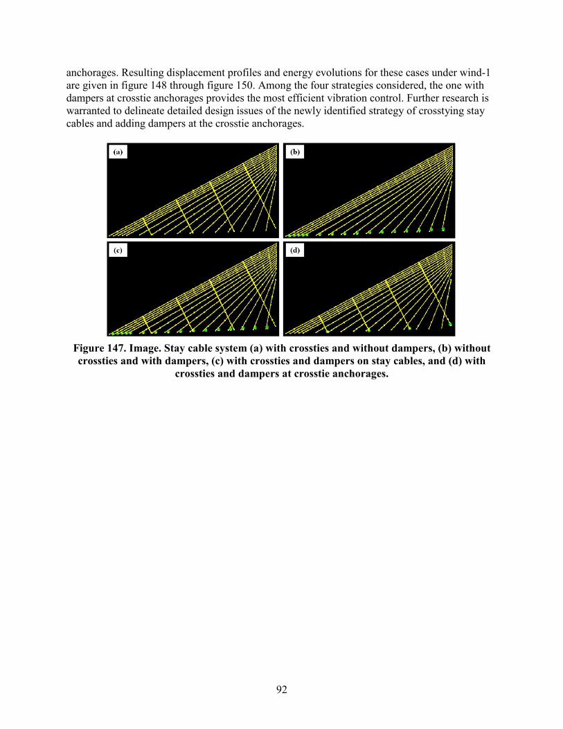
anchorages. Resulting displacement profiles and energy evolutions for these cases under wind-1 are given in figure 148 through figure 150. Among the four strategies considered, the one with dampers at crosstie anchorages provides the most efficient vibration control. Further research is warranted to delineate detailed design issues of the newly identified strategy of crosstying stay cables and adding dampers at the crosstie anchorages.

Figure 147. Image. Stay cable system (a) with crossties and without dampers, (b) without crossties and with dampers, (c) with crossties and dampers on stay cables, and (d) with

crossties and dampers at crosstie anchorages.

92

Figure 148. Graph. Displacement profile computed at mid-span of the longest cable

(a) with crossties and without dampers, (b) without crossties and with dampers, (c) with crossties and dampers on stay cables, and (d) with crossties and dampers at crosstie

anchorages.

Figure 149. Graph. Displacement profile computed at quarter-span of the longest cable (a) with crossties and without dampers, (b) without crossties and with dampers, (c) with

crossties and dampers on stay cables, and (d) with crossties and dampers at crosstie anchorages.

93

Figure 150. Graph. Energy evolution of a cable system (a) with crossties and without

dampers, (b) without crossties and with dampers, (c) with crossties and dampers on stay cables, and (d) with crossties and dampers at crosstie anchorages.

94

CHAPTER 8: CONCLUSIONS

A study on wind-induced vibration of stay cables equipped with different types of mitigation measures was conducted through numerical simulations and analyses. The use of transverse crossties, external dampers, and a combination of the two as mitigation measures were analyzed with respect to their relative merits and shortcomings. Explicit time-history analysis of the behavior of stay systems subjected to realistic wind events was performed as well as a sensitivity study to assess the influence of parameters involved in the design of these measures. The following summary highlights the findings and conclusions drawn from the current study:

• Crossties, in general, are effective in the mitigation of in-plane vibration of stay cables. However, the performance of a crosstied cable network is sensitive to the frequency contents of the input wind profile.

• Crossties are particularly effective in suppressing cable vibrations induced by wind events containing appreciable low-frequency components.

• The performance of a crosstied stay cable system is not necessarily proportional to the quantity (or the number of lines) of crossties. Excessive provision of crossties potentially makes the system susceptible to large-amplitude vibrations under highly turbulent wind events.

• Oversized (or large diameter) crossties make the system overly rigid, rendering the system vulnerable to high-frequency local vibration modes. Crosstie grounding increases the natural frequencies of the system’s global modes of vibration.

• In-plane performance of a crosstied cable network is insensitive to the pre-tension level of crossties as long as this pre-tension level is high enough to prevent slackening of crossties under design wind events. Out-of-plane performance, however, is affected by the pre-tension level of crossties.

• External dampers, in general, are effective in suppressing stay cable vibrations via dissipation of vibration energies of the stay system. However, the efficiency of dampers depends on the spectral properties of the input wind profile.

• Viscous dampers are particularly effective in controlling stay cable vibrations induced by highly turbulent wind flows containing appreciable high-frequency components.

• The effect of a combined use of cable crossties and external dampers is not necessarily the sum of the effects of their independent uses, its efficacy depending on the layout of the crossties and dampers and on the spectral properties of input wind profiles.

• The optimal coefficients of dampers attached to stay cables networked with crossties cannot be determined from the dynamics of individual cable-damper systems. Further research may be needed to develop a practical method for estimating optimal damper coefficients for networked cables.

95

• External dampers installed at crosstie connections to the deck are found to be very efficient in dissipating the vibration energies of a crosstied stay system, constituting an excellent mitigation alternative.

96

CHAPTER 9: RECOMMENDATIONS FOR FUTURE RESEARCH

Future research in the following areas addressing some of the remaining issues would positively supplement the current project:

• Research on the combined use of external dampers and cable crossties: In particular, viscous dampers attached to the crosstie anchorages have been identified as a potentially efficient mitigation strategy. This strategy needs to be further investigated before the concept can be transformed into a mitigation measure that can be implemented. For example, determination of optimal damper coefficients and spring constants (for retraction springs) is one of the issues that needs to be resolved.

• Research on other potentially viable types of external dampers: Viscous or hydraulic dampers have been most commonly specified as external dampers for controlling stay cable vibrations. Despite their widespread use, viscous dampers have been reported to have weaknesses in terms of long-term durability and maintenance requirements. Other types of dampers, such as viscoelastic dampers and friction dampers, have certain strengths over viscous dampers and have been successfully used in other areas of application including wind mitigation of high-rise buildings and seismic mitigation of highway bridges. For example, viscoelastic solid dampers are known to offer optimal damping for a broad range of frequencies (or vibration modes), and friction dampers offer threshold vibration amplitudes below which dampers remain unengaged, resulting in elongated longevity of the dampers. Viscoelastic solid dampers and friction dampers are generally viewed as less demanding in terms of maintenance requirement than viscous dampers.

• Development of a set of additional input wind profiles and testing the effectiveness of the mitigation strategies under these profiles: The effectiveness of various vibration mitigation strategies have been tested using a limited number of input wind profiles. Expanding the scope of wind profiles would allow more reliable conclusions to be drawn regarding the effectiveness of such mitigation strategies.

• Research on the parametric vibration of a cable/deck/tower system: Current research is based on the simplifying assumption that the deck and tower are fixed or immovable with respect to stay cables. Recent studies by others suggest that the vibration of the bridge deck or tower could significantly affect the vibration of stay cables subjected to wind flow. Finite element analysis of an extended domain including the deck, tower, and stay cables may be carried out by expanding the existing analysis model. Clarification of this issue would add a substantial value to the current research study.

97

REFERENCES

1. Post-Tensioning Institute. (2012). Recommendations for Stay Cable Design, Testing, and Installation, Sixth Edition, Post-Tensioning Institute, Farmington Hills, MI.

2. Bosch, H.R. (2000). “Rain/Wind-Induced Vibration of Bridge Cables in the United States,” Proceedings of the 32nd Joint Meeting of the U.S.-Japan Panel on Wind and Seismic Effects, National Institute of Standards and Technology, Gaithersburg, MD.

3. Kumarasena, S., Jones, N.P., Irwin, P., and Taylor, P. (2007). Wind Induced Vibration of Stay Cables, Report No. FHWA-HRT-05-083, Federal Highway Administration, McLean, VA.

4. Graff, K.F. (1975). Wave Motion in Elastic Solids, Oxford University Press, United Kingdom.

5. Zui H., Shinke, T., and Namita, Y. (1996). “Practical Formulas for Estimation of Cable Tension by Vibration Method,” Journal of Structural Engineering, ASCE, 122(6), 651–656.

6. Tabatabai, H. and Mehrabi, A. (1998). “Unified Finite Difference Formulation for Free Vibration of Cable,” Journal of Structural Engineering, ASCE, 124, 1313–1322.

7. Irvine, M. (1992). Cable Structures, Dover Publications, New York City, NY.

8. SAP2000®. (2004). Structural Analysis Program, Nonlinear Version 9.0, Computers and Structures, Inc., Berkeley, CA.

9. Caracoglia, L. and Jones, N.P. (2005). “In-Plane Dynamic Behavior of Cable Networks Part 1: Formulation and Basic Solutions,” Journal of Sound and Vibration, Elsevier, 279, 969–991.

10. Caracoglia, L. and Jones, N.P. (2005). “In-Plane Dynamic Behavior of Cable Networks Part 2: Prototype Prediction and Validation,” Journal of Sound and Vibration, Elsevier, 279, 993–1014.

11. Gimsing, N.J. (1983). Cable Supported Bridges: Concept and Design, Wiley, New York, NY.

12. Caracoglia, L. and Jones, N.P. (2003). “Dynamics of Stay-Cable Systems and Cross-Tied Networks,” Proceedings of the 5th International Symposium on Cable Dynamics, AIM, Santa Margherita, Italy, 437–444.

13. Caracoglia, L. and Jones, N.P. (2004). “Selection of an Optimized Cable Network System Configuration,” Proceedings of the 17th Engineering Mechanics Conference, CD-ROM, ASCE, University of Delaware, Newark, DE.

99

14. Abdel-Ghaffar, A.M. and Khalifa, M.A. (1991). “Importance of Cable Vibration in Dynamics of Cable-Stayed Bridges,” Journal of Engineering Mechanics, ASCE, 117, 2571–2589.

15. Krenk, S. (2000). “Vibrations of a Taut Cable with External Damper,” Journal of Applied Mechanics, ASME, 67(4), 772–776.

16. Tschoegl, N.W. (1989). The Phenomenological Theory of Linear Viscoelastic Behavior, Springer-Verlag, Berlin, Germany.

100

BIBLIOGRAPHY

1. Krenk, S. and Høgsberg, J.R. (2005). “Damping of Cables by a Transverse Force,” Journal of Engineering Mechanics, ASCE, 131(4), 340–348.

2. Main, J.A. and Jones, N.P. (2002). “Free Vibrations of a Taut Cable with Attached Damper I: Linear Viscous Damper,” Journal of Engineering Mechanics, ASCE, 128(10), 1062–1071.

3. Main, J.A. and Jones, N.P. (2002). “Free Vibrations of a Taut Cable with Attached Damper II: Nonlinear Damper,” Journal of Engineering Mechanics, ASCE, 128(10), 1072–1081.

4. Main, J.A. and Jones, N.P. (2001). “Evaluation of Viscous Dampers for Stay-Cable Vibration Mitigation,” Journal of Bridge Engineering. ASCE, 6(6), 385–397.

5. Pacheco, B.M., Fujino, Y., and Sulekh, A. (1993). “Estimation Curve for Modal Damping in Stay Cables with Viscous Damper,” Journal of Structural Engineering, ASCE, 119(6), 1961–1979.

101

HRDI-50/08-14(WEB)E

mitigation of wind-induced vibration of stay cables ... . cable-stayed bridges have become the form...

Documents