mixed-effects modeling with crossed random ... - jake westfalljakewestfall.org/misc/bdb2008.pdf ·...

Mixed-e!ects modeling with crossed random e!ectsfor subjects and items

R.H. Baayen a,*, D.J. Davidson b, D.M. Bates c

a University of Alberta, Edmonton, Department of Linguistics, Canada T6G 2E5b Max Planck Institute for Psycholinguistics, P.O. Box 310, 6500 AH Nijmegen, The Netherlands

c University of Wisconsin, Madison, Department of Statistics, WI 53706-168, USA

Received 15 February 2007; revision received 13 December 2007Available online 3 March 2008

Abstract

This paper provides an introduction to mixed-e!ects models for the analysis of repeated measurement data with sub-jects and items as crossed random e!ects. A worked-out example of how to use recent software for mixed-e!ects mod-eling is provided. Simulation studies illustrate the advantages o!ered by mixed-e!ects analyses compared to traditionalanalyses based on quasi-F tests, by-subjects analyses, combined by-subjects and by-items analyses, and random regres-sion. Applications and possibilities across a range of domains of inquiry are discussed.! 2007 Elsevier Inc. All rights reserved.

Keywords: Mixed-e!ects models; Crossed random e!ects; Quasi-F; By-item; By-subject

Psycholinguists and other cognitive psychologists useconvenience samples for their experiments, often basedon participants within the local university community.When analyzing the data from these experiments, partic-ipants are treated as random variables, because theinterest of most studies is not about experimental e!ectspresent only in the individuals who participated in theexperiment, but rather in e!ects present in languageusers everywhere, either within the language studied,or human language users in general. The di!erencesbetween individuals due to genetic, developmental, envi-ronmental, social, political, or chance factors are mod-eled jointly by means of a participant random e!ect.

A similar logic applies to linguistic materials. Psych-olinguists construct materials for the tasks that theyemploy by a variety of means, but most importantly,most materials in a single experiment do not exhaustall possible syllables, words, or sentences that could befound in a given language, and most choices of languageto investigate do not exhaust the possible languages thatan experimenter could investigate. In fact, two core prin-ciples of the structure of language, the arbitrary (andhence statistical) association between sound and mean-ing and the unbounded combination of finite lexicalitems, guarantee that a great many language materialsmust be a sample, rather than an exhaustive list. Thespace of possible words, and the space of possible sen-tences, is simply too large to be modeled by any othermeans. Just as we model human participants as randomvariables, we have to model factors characterizing theirspeech as random variables as well.

0749-596X/$ - see front matter ! 2007 Elsevier Inc. All rights reserved.doi:10.1016/j.jml.2007.12.005

* Corresponding author. Fax: +1 780 4920806.E-mail addresses: [email protected] (R.H. Baayen),

[email protected] (D.J. Davidson), [email protected] (D.M. Bates).

Available online at www.sciencedirect.com

Journal of Memory and Language 59 (2008) 390–412

Journal ofMemory and

Language

www.elsevier.com/locate/jml

mailto:[email protected]

mailto:[email protected]

Clark (1973) illuminated this issue, sparked by thework of Coleman (1964), by showing how languageresearchers might generalize their results to the largerpopulation of linguistic materials from which they sam-ple by testing for statistical significance of experimentalcontrasts with participants and items analyses. Clark’soft-cited paper presented a technical solution to thismodeling problem, based on statistical theory and com-putational methods available at the time (e.g., Winer,1971). This solution involved computing a quasi-F sta-tistic which, in the simplest-to-use form, could beapproximated by the use of a combined minimum-F sta-tistic derived from separate participants (F1) and items(F2) analyses. In the 30+ years since, statistical tech-niques have expanded the space of possible solutionsto this problem, but these techniques have not yet beenapplied widely in the field of language and memory stud-ies. The present paper discusses an alternative known asa mixed e!ects model approach, based on maximumlikelihood methods that are now in common use inmany areas of science, medicine, and engineering (see,e.g., Faraway, 2006; Fielding & Goldstein, 2006; Gil-mour, Thompson, & Cullis, 1995; Goldstein, 1995; Pin-heiro & Bates, 2000; Snijders & Bosker, 1999).

Software for mixed-e!ects models is now widelyavailable, in specialized commercial packages such asMLwiN (MLwiN, 2007) and ASReml (Gilmour, Gogel,Cullis, Welham, & Thompson, 2002), in general com-mercial packages such as SAS and SPSS (the’mixed’ proce-dures), and in the open source statistical programmingenvironment R (Bates, 2007). West, Welch, and Ga"lech-ki (2007) provide a guide to mixed models for five di!er-ent software packages.

In this paper, we introduce a relatively recent devel-opment in computational statistics, namely, the possibil-ity to include subjects and items as crossed, independent,random e!ects, as opposed to hierarchical or multilevelmodels in which random e!ects are assumed to benested. This distinction is sometimes absent in generaltreatments of these models, which tend to focus onnested models. The recent textbook by West et al.(2007), for instance, does not discuss models withcrossed random e!ects, although it clearly distinguishesbetween nested and crossed random e!ects, and advisesthe reader to make use of the lmer() function in R, thesoftware (developed by the third author) that we intro-duce in the present study, for the analysis of crosseddata.

Traditional approaches to random e!ects modelingsu!er multiple drawbacks which can be eliminated byadopting mixed e!ect linear models. These drawbacksinclude (a) deficiencies in statistical power related tothe problems posed by repeated observations, (b) thelack of a flexible method of dealing with missing data,(c) disparate methods for treating continuous and cate-gorical responses, as well as (d) unprincipled methods

of modeling heteroskedasticity and non-sphericalerror variance (for either participants or items). Meth-ods for estimating linear mixed e!ect models haveaddressed each of these concerns, and o!er a betterapproach than univariate ANOVA or ordinary leastsquares regression.

In what follows, we first introduce the concepts andformalism of mixed e!ects modeling.

Mixed e!ects model concepts and formalism

The concepts involved in a linear mixed e!ects modelwill be introduced by tracing the data analysis path of asimple example. Assume an example data set with threeparticipants s1, s2 and s3 who each saw three items w1,w2, w3 in a priming lexical decision task under bothshort and long SOA conditions. The design, the RTsand their constituent fixed and random e!ects compo-nents are shown in Table 1.

This table is divided into three sections. The left-most section lists subjects, items, the two levels ofthe SOA factor, and the reaction times for each com-bination of subject, item and SOA. This section repre-sents the data available to the analyst. The remainingsections of the table list the e!ects of SOA and theproperties of the subjects and items that underly theRTs. Of these remaining sections, the middle sectionlists the fixed e!ects: the intercept (which is the samefor all observations) and the e!ect of SOA (a 19 msprocessing advantage for the short SOA condition).The right section of the table lists the random e!ectsin the model. The first column in this section listsby-item adjustments to the intercept, and the secondcolumn lists by-subject adjustments to the intercept.The third column lists by-subject adjustments to thee!ect of SOA. For instance, for the first subject thee!ect of a short SOA is attenuated by 11 ms. The finalcolumn lists the by-observation noise. Note that inthis example we did not include by-item adjustmentsto SOA, even though we could have done so. In theterminology of mixed e!ects modeling, this data setis characterized by random intercepts for both subjectand item, and by by-subject random slopes (but noby-item random slopes) for SOA.

Formally, this dataset is summarized in (1).

yij ! Xijb" Sisi "Wjwj " !ij #1$

The vector yij represents the responses of subject i toitem j. In the present example, each of the vectors yij

comprises two response latencies, one for the shortand one for the long SOA. In (1), Xij is the design ma-trix, consisting of an initial column of ones and followedby columns representing factor contrasts and covariates.For the present example, the design matrix for each sub-ject-item combination has the simple form

R.H. Baayen et al. / Journal of Memory and Language 59 (2008) 390–412 391

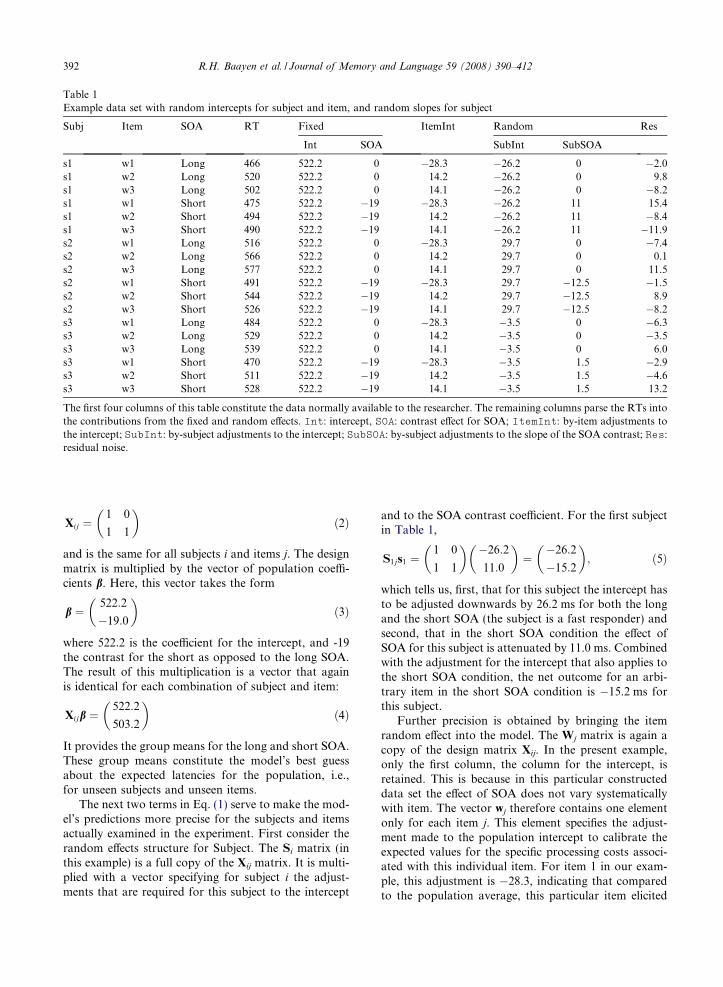
Xij !1 0

1 1

! "#2$

and is the same for all subjects i and items j. The designmatrix is multiplied by the vector of population coe#-cients b. Here, this vector takes the form

b !522:2

%19:0

! "#3$

where 522.2 is the coe#cient for the intercept, and -19the contrast for the short as opposed to the long SOA.The result of this multiplication is a vector that againis identical for each combination of subject and item:

Xijb !522:2

503:2

! "#4$

It provides the group means for the long and short SOA.These group means constitute the model’s best guessabout the expected latencies for the population, i.e.,for unseen subjects and unseen items.

The next two terms in Eq. (1) serve to make the mod-el’s predictions more precise for the subjects and itemsactually examined in the experiment. First consider therandom e!ects structure for Subject. The Si matrix (inthis example) is a full copy of the Xij matrix. It is multi-plied with a vector specifying for subject i the adjust-ments that are required for this subject to the intercept

and to the SOA contrast coe#cient. For the first subjectin Table 1,

S1js1 !1 0

1 1

! " %26:2

11:0

! "!%26:2

%15:2

! "; #5$

which tells us, first, that for this subject the intercept hasto be adjusted downwards by 26.2 ms for both the longand the short SOA (the subject is a fast responder) andsecond, that in the short SOA condition the e!ect ofSOA for this subject is attenuated by 11.0 ms. Combinedwith the adjustment for the intercept that also applies tothe short SOA condition, the net outcome for an arbi-trary item in the short SOA condition is %15.2 ms forthis subject.

Further precision is obtained by bringing the itemrandom e!ect into the model. The Wj matrix is again acopy of the design matrix Xij. In the present example,only the first column, the column for the intercept, isretained. This is because in this particular constructeddata set the e!ect of SOA does not vary systematicallywith item. The vector wj therefore contains one elementonly for each item j. This element specifies the adjust-ment made to the population intercept to calibrate theexpected values for the specific processing costs associ-ated with this individual item. For item 1 in our exam-ple, this adjustment is %28.3, indicating that comparedto the population average, this particular item elicited

Table 1Example data set with random intercepts for subject and item, and random slopes for subject

Subj Item SOA RT Fixed ItemInt Random Res

Int SOA SubInt SubSOA

s1 w1 Long 466 522.2 0 %28.3 %26.2 0 %2.0s1 w2 Long 520 522.2 0 14.2 %26.2 0 9.8s1 w3 Long 502 522.2 0 14.1 %26.2 0 %8.2s1 w1 Short 475 522.2 %19 %28.3 %26.2 11 15.4s1 w2 Short 494 522.2 %19 14.2 %26.2 11 %8.4s1 w3 Short 490 522.2 %19 14.1 %26.2 11 %11.9s2 w1 Long 516 522.2 0 %28.3 29.7 0 %7.4s2 w2 Long 566 522.2 0 14.2 29.7 0 0.1s2 w3 Long 577 522.2 0 14.1 29.7 0 11.5s2 w1 Short 491 522.2 %19 %28.3 29.7 %12.5 %1.5s2 w2 Short 544 522.2 %19 14.2 29.7 %12.5 8.9s2 w3 Short 526 522.2 %19 14.1 29.7 %12.5 %8.2s3 w1 Long 484 522.2 0 %28.3 %3.5 0 %6.3s3 w2 Long 529 522.2 0 14.2 %3.5 0 %3.5s3 w3 Long 539 522.2 0 14.1 %3.5 0 6.0s3 w1 Short 470 522.2 %19 %28.3 %3.5 1.5 %2.9s3 w2 Short 511 522.2 %19 14.2 %3.5 1.5 %4.6s3 w3 Short 528 522.2 %19 14.1 %3.5 1.5 13.2

The first four columns of this table constitute the data normally available to the researcher. The remaining columns parse the RTs intothe contributions from the fixed and random e!ects. Int: intercept, SOA: contrast e!ect for SOA; ItemInt: by-item adjustments tothe intercept; SubInt: by-subject adjustments to the intercept; SubSOA: by-subject adjustments to the slope of the SOA contrast; Res:residual noise.

392 R.H. Baayen et al. / Journal of Memory and Language 59 (2008) 390–412

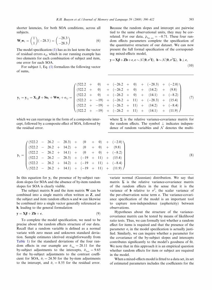
shorter latencies, for both SOA conditions, across allsubjects.

Wjw1 !1

1

! "%28:3# $ !

%28:3

%28:3

! "#6$

The model specification (1) has as its last term the vectorof residual errors !ij, which in our running example hastwo elements for each combination of subject and item,one error for each SOA.

For subject 1, Eq. (1) formalizes the following vectorof sums,

which we can rearrange in the form of a composite inter-cept, followed by a composite e!ect of SOA, followed bythe residual error.

In this equation for y1 the presence of by-subject ran-dom slopes for SOA and the absence of by-item randomslopes for SOA is clearly visible.

The subject matrix S and the item matrix W can becombined into a single matrix often written as Z, andthe subject and item random e!ects s and w can likewisebe combined into a single vector generally referenced asb, leading to the general formulation

y ! Xb" Zb" !: #9$

To complete the model specification, we need to beprecise about the random e!ects structure of our data.Recall that a random variable is defined as a normalvariate with zero mean and unknown standard devia-tion. Sample estimates (derived straightforwardly fromTable 1) for the standard deviations of the four ran-dom e!ects in our example are rsint

! 28:11 for theby-subject adjustments to the intercepts, rssoa ! 9:65for the by-subject adjustments to the contrast coe#-cient for SOA, ri ! 24:50 for the by-item adjustmentsto the intercept, and r! ! 8:55 for the residual error.

Because the random slopes and intercept are pairwisetied to the same observational units, they may be cor-related. For our data, qsint; soa

! %0:71. These four ran-dom e!ects parameters complete the specification ofthe quantitative structure of our dataset. We can nowpresent the full formal specification of the correspond-ing mixed-e!ects model,

y!Xb"Zb"!;!&N #0;r2I$; b&N #0;r2R$; b? !;#10$

where R is the relative variance-covariance matrix forthe random e!ects. The symbol \ indicates indepen-dence of random variables and N denotes the multi-

variate normal (Gaussian) distribution. We say thatmatrix R is the relative variance-covariance matrixof the random e!ects in the sense that it is thevariance of b relative to r2, the scalar variance ofthe per-observation noise term !. The variance-covari-ance specification of the model is an important toolto capture non-independence (asphericity) betweenobservations.

Hypotheses about the structure of the variance-covariance matrix can be tested by means of likelihoodratio tests. Thus, we can formally test whether a randome!ect for items is required and that the presence of theparameter ri in the model specification is actually justi-fied. Similarly, we can inquire whether a parameter forthe covariance of the by-subject slopes and interceptscontributes significantly to the model’s goodness of fit.We note that in this approach it is an empirical questionwhether random e!ects for item or subject are requiredin the model.

When a mixed-e!ects model is fitted to a data set, its setof estimated parameters includes the coe#cients for the

y1 ! y1j ! X1jb" Ss1 "Wwj " !1j !

#522:2 " 0$ " #%26:2 " 0$ " #%28:3$ " #%2:0$#522:2 " 0$ " #%26:2 " 0$ " #14:2$ " #9:8$#522:2 " 0$ " #%26:2 " 0$ " #14:1$ " #%8:2$#522:2 " %19$ " #%26:2 " 11$ " #%28:3$ " #15:4$#522:2 " %19$ " #%26:2 " 11$ " #14:2$ " #%8:4$#522:2 " %19$ " #%26:2 " 11$ " #14:1$ " #11:9$

0

BBBBBBBB@

1

CCCCCCCCA

#7$

y1 !

#522:2 % 26:2 % 28:3$ " #0 " 0$ " #%2:0$#522:2 % 26:2 " 14:2$ " #0 " 0$ " #9:8$#522:2 % 26:2 " 14:1$ " #0 " 0$ " #%8:2$#522:2 % 26:2 % 28:3$ " #%19 " 11$ " #15:4$#522:2 % 26:2 " 14:2$ " #%19 " 11$ " #%8:4$#522:2 % 26:2 " 14:1$ " #%19 " 11$ " #11:9$

0

BBBBBBBB@

1

CCCCCCCCA

#8$


fixed e!ects on the one hand, and the standard deviationsand correlations for the random e!ects on the other hand.The individual values of the adjustments made to inter-cepts and slopes are calculated once the random-e!ectsparameters have been estimated. Formally, these adjust-ments, referenced as Best Linear Unbiased Predictors(or BLUPs), are not parameters of the model.

Data analysis

We illustrate mixed-e!ects modeling with R, an open-source language and environment for statistical comput-ing (R development core team, 2007), freely available athttp://cran.r-project.org. The lme4 package(Bates, 2005; Bates & Sarkar, 2007) o!ers fast and reliablealgorithms for parameter estimation (see also West et al.,2007:14) as well as tools for evaluating the model (usingMarkov chain Monte Carlo sampling, as explainedbelow).

Input data for R should have the structure of the firstblock in Table 1, together with an initial header linespecifying column names. The data for the first subjecttherefore should be structured as follows, using what isknown as the long data format in R (and as the univar-iate data format in SPSS):

Subj Item SOA RT

1 s1 w1 short 4752 s1 w2 short 4943 s1 w3 short 4904 s1 w1 long 4665 s1 w2 long 5206 s1 w3 long 502

We load the data, here simply an ASCII text file, intoR with

> priming = read.table("ourdata.txt",header = TRUE)

SPSS data files (if brought into the long format withinSPSS) can be loaded with read.spss and csv tables(in long format) are loaded with read.csv. We fit themodel of Eq. (10) to the data with

> priming.lmer = lmer(RT & SOA + (1jItem) +(1 + SOAjSubj), data = priming)

The dependent variable, RT, appears to the left of thetilde operator (&), which is read as ‘‘depends on” or ‘‘isa function of”. The main e!ect of SOA, our fixed e!ect,is specified to the right of the tilde. The random interceptfor Item is specified with (1|Item), which is read as arandom e!ect introducing adjustments to the intercept(denoted by 1) conditional on or grouped by Item. Therandom e!ects for Subject are specified as(1+SOA|Subject). This notation indicates, first of

all, that we introduce by-subject adjustments to the inter-cept (again denoted by 1) as well as by-subject adjust-ments to SOA. In other words, this model includes by-subject and by-item random intercepts, and by-subjectrandom slopes for SOA. This notation also indicates thatthe variances for the two levels of SOA are allowed to bedi!erent. In other words, it models potential by-subjectheteroskedasticity with respect to SOA. Finally, this spec-ification includes a parameter estimating the correlationqsint; soa

of the by-subject random e!ects for slope andintercept.

A summary of the model is obtained with

> summary (priming.lmer)Linear mixed-effects model fit by REML

Formula : RT&SOA+(1jItem)+(1+SOAjSubj)Data : primingAIC BIC logLik ML

devianceREMLdeviance

150.0 155.4 %69.02 151.4 138.0Random effects :

Groups Name Variance Std.Dev Corr

Item (Intercept) 613.73 24.774Subj (Intercept) 803.07 28.338

SOAshort 136.46 11.682 %1.000Residual 102.28 10.113

number of obs : 18, groups : Item, 3; Subj, 3Fixed effects :

Estimate Std.Error

t value

(Intercept) 522.111 21.992 23.741SOAshort %18.889 8.259 %2.287

The summary first mentions that the model is fittedusing restricted maximum likelihood estimation (REML),a modification of maximum likelihood estimation that ismore precise for mixed-e!ects modeling. Maximum like-lihood estimation seeks to find those parameter valuesthat, given the data and our choice of model, make themodel’s predicted values most similar to the observedvalues. Discussion of the technical details of model fit-ting is beyond the scope of this paper. However, in theAppendix we provide some indication of the kind ofissues involved.

The summary proceeds with repeating the modelspecification, and then lists various measures of good-ness of fit. The remainder of the summary containstwo subtables, one for the random e!ects, and one forthe fixed e!ects.

The subtable for the fixed-e!ects shows that theestimates for slope and the contrast coe#cient forSOA are right on target: 522.11 for the intercept (com-pare 522.2 in Table 1), and -18.89 (compare -19.0).For each coe#cient, its standard error and t-statisticare listed.


http://cran.r-project.org

Turning to the subtable of random e!ects, we observethat the first column lists the main grouping factors:Item, Subj and the observation noise (Residual).The second column specifies whether the random e!ectconcerns the intercept or a slope. The third columnreports the variances, and the fourth column the squareroots of these variances, i.e., the corresponding standarddeviations. The sample standard deviations calculatedabove on the basis of Table 1 compare well with themodel estimates, as shown in Table 2.

The high correlation of the intercept and slope for thesubject random e!ects (%1.00) indicates that the modelhas been overparameterized. We first simplify the modelby removing the correlation parameter and by assuming

homoskedasticity for the subjects with respect to theSOA conditions, as follows:

> priming.lmer1 = lmer(RT & SOA + (1jItem) +(1jSubj) + (1j SOA:Subj), data =priming)> print(priming.lmer1, corr = FALSE)

Random effects

Groups Name Variance Std.Dev.

SOA:Subj (Intercept) 34.039 5.8343Subj (Intercept) 489.487 22.1243Item (Intercept) 625.623 25.0125Residual 119.715 10.9414

number of obs: 18, groups: SOA:Subj, 6; Subj, 3; Item, 3Fixed effects:

Estimate Std. Error t value


(Here and in the examples to follow, we abbreviated theR output.) The variance for the by-subject adjustmentsfor SOA is small, and potentially redundant, so we fur-

ther simplify to a model with only random intercepts forsubject:

> priming.lmer2 = lmer(RT & SOA + (1j Item) +(1jSubj), data = priming)

In order to verify that this most simple model isjustified, we carry out a likelihood ratio test (see,e.g., Pinheiro & Bates, 2000, p. 83) that comparesthe most specific model priming.lmer2 (which setsq to the specific value of zero and assumes homoske-dasticity) with the more general model prim-ing.lmer (which does not restrict q a priori andexplicitly models heteroskedasticity). The likelihoodof the more general model (Lg) should be greater thanthe likelihood of the more specific model (Ls), andhence the likelihood ratio test statistic 2log(Lg/Ls) > 0. If g is the number of parameters for the gen-eral model, and s the number of parameters for therestricted model, then the asymptotic distribution ofthe likelihood ratio test statistic, under the nullhypothesis that the restricted model is su#cient, fol-lows a chi-squared distribution with g-s degrees offreedom. In R, the likelihood ratio test is carried outwith the anova function:

The value listed under Chisq equals twice the di!er-ence between the log-likelihood (listed under logLik)for priming.lmer and that of priming.lmer2.The degrees of freedom for the chi-squared distribution,2, is the di!erence between the number of parameters inthe model (listed under Df). It it clear that the removalof the parameter for the correlation together with theparameter for by-subject random slopes for SOA is jus-tified (X 2

#2$ ! 2:96; p ! 0:228). The summary of the sim-plified model

> print(priming.lmer2, corr = FALSE)Random effects:


Item (Intercept) 607.72 24.652Subj (Intercept) 499.22 22.343Residual 137.35 11.720

number of obs: 18, groups: Item, 3; Subj, 3Fixed effects:



> anova(priming.lmer, priming.lmer2)

Df AIC BIC logLik Chisq Chi Df Pr(>Chisq)

priming.lmer2 4 162.353 165.914 %77.176priming.lmer 6 163.397 168.740 %75.699 2.9555 2 0.2282

Table 2Comparison of sample estimates and model estimates for thedata of Table 1

Parameter Sample Model

ri 24.50 24.774rsint 28.11 28.338rssoa 9.65 11.681r! 8.55 10.113qsint; soa %0.71 %1.00


lists only random intercepts for subject and item, asdesired.

The reader may have noted that summaries for modelobjects fitted with lmer list standard errors and t-statis-tics for the fixed e!ects, but no p-values. This is not with-out reason.

With many statistical modeling techniques we canderive exact distributions for certain statistics calculatedfrom the data and use these distributions to performhypothesis tests on the parameters, or to create confi-dence intervals or confidence regions for the values ofthese parameters. The general class of linear models fitby ordinary least squares is the prime example of sucha well-behaved class of statistical models for which wecan derive exact results, subject to certain assumptionson the distribution of the responses (normal, constantvariance and independent disturbance terms). This gen-eral paradigm provides many of the standard techniquesof modern applied statistics including t-tests and analy-sis of variance decompositions, as well as confidenceintervals based on t-distributions. It is tempting tobelieve that all statistical techniques should provide suchneatly packaged results, but they don’t.

Inferences regarding the fixed-e!ects parameters aremore complicated in a linear mixed-e!ects model thanin a linear model with fixed e!ects only. In a model withonly fixed e!ects we estimate these parameters and oneother parameter which is the variance of the noise thatinfects each observation and that we assume to be inde-pendent and identically distributed (i.i.d.) with a normal(Gaussian) distribution. The initial work by WilliamGossett (who wrote under the pseudonym of ‘‘Student”)on the e!ect of estimating the variance of the distur-bances on the estimates of precision of the sample mean,leading to the t-distribution, and later generalizations bySir Ronald Fisher, providing the analysis of variance,were turning points in 20th century statistics.

When mixed-e!ects models were first examined, inthat days when the computing tools were considerablyless sophisticated than at present, many approximationswere used, based on analogy to fixed-e!ects analysis ofvariance. For example, variance components were oftenestimated by calculating certain mean squares andequating the observed mean square to the correspondingexpected mean square. There is no underlying objective,such as the log-likelihood or the log-restricted-likeli-hood, that is being optimized by such estimates. Theyare simply assumed to be desirable because of the anal-ogy to the results in the analysis of variance. Further-more, the theoretical derivations and correspondingcalculations become formidable in the presence of multi-ple factors, such as both subject and item, associatedwith random e!ects or in the presence of unbalanceddata.

Fortunately, it is now possible to evaluate the maxi-mum likelihood or the REML estimates of the parameters

in mixed-e!ects models reasonably easily and quickly,even for complex models fit to very large observationaldata sets. However, the temptation to perform hypothe-sis tests using t-distributions or F-distributions based oncertain approximations of the degrees of freedom inthese distributions persists. An exact calculation can bederived for certain models with a comparatively simplestructure applied to exactly balanced data sets, such asoccur in text books. In real-world studies the data oftenend up unbalanced, especially in observational studiesbut even in designed experiments where missing datacan and do occur, and the models can be quite compli-cated. The simple formulas for the degrees of freedomfor inferences based on t or F-distributions do not applyin such cases. In fact, the pivotal quantities for suchhypothesis tests do not even have t or F-distributionsin such cases so trying to determine the ‘‘correct” valueof the degrees of freedom to apply is meaningless. Thereare many approximations in use for hypothesis tests inmixed models—the MIXED procedure in SAS o!ers 6 dif-ferent calculations of degrees of freedom in certain tests,each leading to di!erent p-values, but none of them is‘‘correct”.

It is not even obvious how to count the number ofparameters in a mixed-e!ects model. Suppose we have1000 subjects, each exposed to 200 items chosen froma pool of 10000 potential items. If we model the e!ectof subject and item as independent random e!ects weadd two variance components to the model. At the esti-mated parameter values we can evaluate 1000 predictorsof the random e!ects for subject and 10000 predictors ofthe random e!ects for item. Did we only add two param-eters to the model when we incorporated these 11000random e!ects? Or should we say that we added severalthousand parameters that are adjusted to help explainthe observed variation in the data? It is overly simplisticto say that thousands of random e!ects amount to onlytwo parameters. However, because of the shrinkagee!ect in the evaluation of the random e!ects, each ran-dom e!ect does not represent an independent parameter.

Fortunately, we can avoid this issue of countingparameters or, more generally, the issue of approximat-ing degrees of freedom. Recall that the original purposeof the t and F-distributions is to take into account theimprecision in the estimate of the variance of the ran-dom disturbances when formulating inferences regard-ing the fixed-e!ects parameters. We can approach thisproblem in the more general context with Markov chainMonte Carlo (MCMC) simulations. In MCMC simulationswe sample from conditional distributions of parametersubsets in a cycle, thus allowing the variation in oneparameter subset, such as the variance of the randomdisturbances or the variances and covariances of ran-dom e!ects, to be reflected in the variation of otherparameter subsets, such as the fixed e!ects. This is whatthe t and F-distributions accomplish in the case of mod-


els with fixed-e!ects only. Crucially, the MCMC techniqueapplies to more general models and to data sets witharbitrary structure.

Informally, we can conceive of Markov chain MonteCarlo (MCMC) sampling from the posterior distributionof the parameters (see, e.g., Andrieu, de Freitas, Doucet,& Jordan, 2003, for a general introduction to MCMC) as arandom walk in parameter space. Each mixed e!ectsmodel is associated with a parameter vector, which canbe divided into three subsets,

1. the variance, r2, of the per-observation noise term,2. the parameters that determine the variance-covari-

ance matrix of the random e!ects, and3. the random e!ects b and the fixed e!ects b.

Conditional on the other two subsets and on thedata, we can sample directly from the posterior distribu-tion of the remaining subset. For the first subset we sam-ple from a chi-squared distribution conditional on the

current residuals. The prior for the variances and covari-ances of the random e!ects is chosen so that for the sec-ond subset we sample from a Wishart distribution.Finally, conditional on the first two subsets and on thedata the sampling for the third subset is from a multivar-iate normal distribution. The details are less importantthan the fact that these are well-accepted ‘‘non-informa-tive” priors for these parameters. Starting from the REML

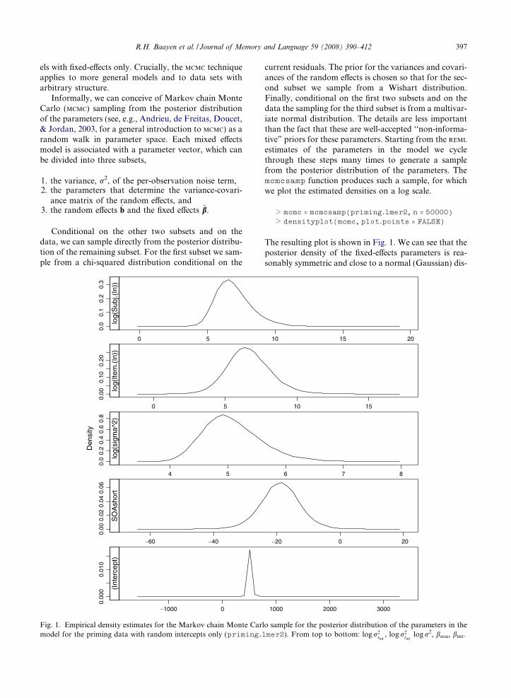
estimates of the parameters in the model we cyclethrough these steps many times to generate a samplefrom the posterior distribution of the parameters. Themcmcsamp function produces such a sample, for whichwe plot the estimated densities on a log scale.

> mcmc = mcmcsamp(priming.lmer2, n = 50000)> densityplot(mcmc, plot.points = FALSE)

The resulting plot is shown in Fig. 1. We can see that theposterior density of the fixed-e!ects parameters is rea-sonably symmetric and close to a normal (Gaussian) dis-

Den

sity

0.00

00.

010

!1000 0 1000 2000 3000

(Int

erce

pt)

0.00

0.02

0.04

0.06

!60 !40 !20 0 20

SO

Ash

ort

0.0

0.2

0.4

0.6

0.8

4 5 6 7 8

log(

sigm

a^2)

0.00

0.10

0.20

0 5 10 15

log(

Item

.(In

))

0.0

0.1

0.2

0.3

0 5 10 15 20

log(

Sub

j.(In

))

Fig. 1. Empirical density estimates for the Markov chain Monte Carlo sample for the posterior distribution of the parameters in themodel for the priming data with random intercepts only (priming.lmer2). From top to bottom: log r2

sint, log r2

iintlog r2, bsoa, bint.


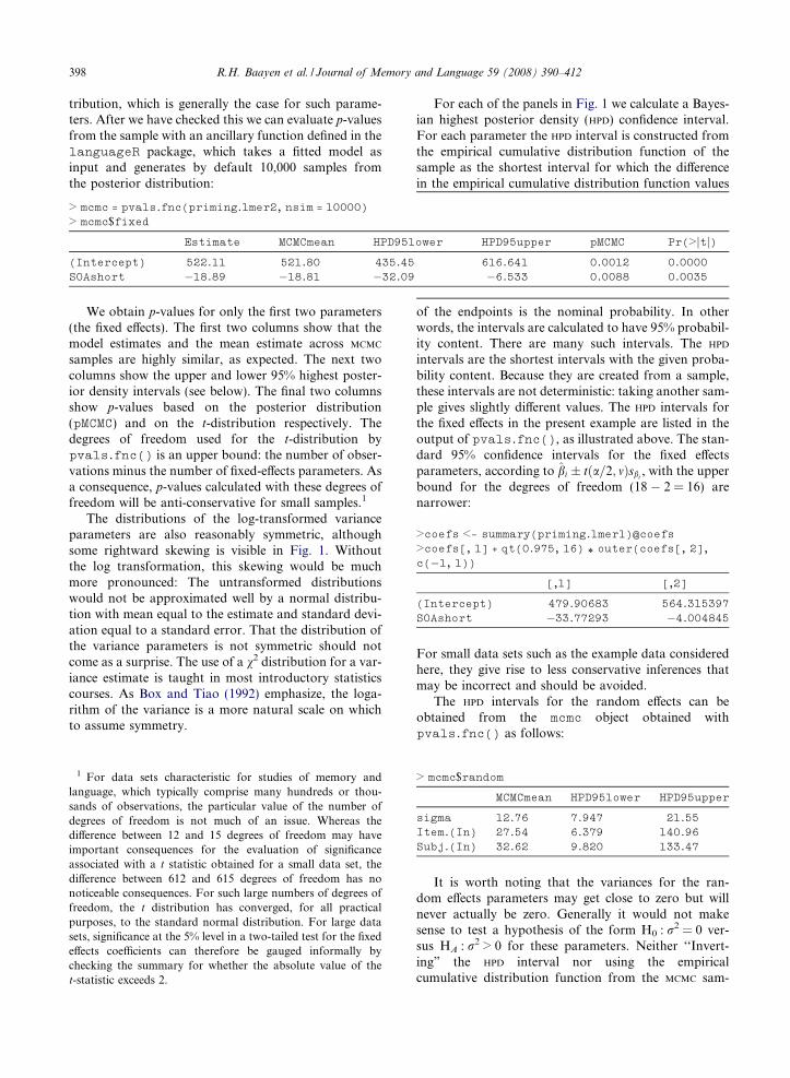
tribution, which is generally the case for such parame-ters. After we have checked this we can evaluate p-valuesfrom the sample with an ancillary function defined in thelanguageR package, which takes a fitted model asinput and generates by default 10,000 samples fromthe posterior distribution:

We obtain p-values for only the first two parameters(the fixed e!ects). The first two columns show that themodel estimates and the mean estimate across MCMC

samples are highly similar, as expected. The next twocolumns show the upper and lower 95% highest poster-ior density intervals (see below). The final two columnsshow p-values based on the posterior distribution(pMCMC) and on the t-distribution respectively. Thedegrees of freedom used for the t-distribution bypvals.fnc() is an upper bound: the number of obser-vations minus the number of fixed-e!ects parameters. Asa consequence, p-values calculated with these degrees offreedom will be anti-conservative for small samples.1

The distributions of the log-transformed varianceparameters are also reasonably symmetric, althoughsome rightward skewing is visible in Fig. 1. Withoutthe log transformation, this skewing would be muchmore pronounced: The untransformed distributionswould not be approximated well by a normal distribu-tion with mean equal to the estimate and standard devi-ation equal to a standard error. That the distribution ofthe variance parameters is not symmetric should notcome as a surprise. The use of a v2 distribution for a var-iance estimate is taught in most introductory statisticscourses. As Box and Tiao (1992) emphasize, the loga-rithm of the variance is a more natural scale on whichto assume symmetry.

For each of the panels in Fig. 1 we calculate a Bayes-ian highest posterior density (HPD) confidence interval.For each parameter the HPD interval is constructed fromthe empirical cumulative distribution function of thesample as the shortest interval for which the di!erencein the empirical cumulative distribution function values

of the endpoints is the nominal probability. In otherwords, the intervals are calculated to have 95% probabil-ity content. There are many such intervals. The HPD

intervals are the shortest intervals with the given proba-bility content. Because they are created from a sample,these intervals are not deterministic: taking another sam-ple gives slightly di!erent values. The HPD intervals forthe fixed e!ects in the present example are listed in theoutput of pvals.fnc(), as illustrated above. The stan-dard 95% confidence intervals for the fixed e!ectsparameters, according to bi ' t#a=2; m$sbi

, with the upperbound for the degrees of freedom (18 % 2 = 16) arenarrower:

>coefs <- summary(priming.lmer1)@coefs>coefs[, 1] + qt(0.975, 16) * outer(coefs[, 2],c(%1, 1))

[,1] [,2]

(Intercept) 479.90683 564.315397SOAshort %33.77293 %4.004845

For small data sets such as the example data consideredhere, they give rise to less conservative inferences thatmay be incorrect and should be avoided.

The HPD intervals for the random e!ects can beobtained from the mcmc object obtained withpvals.fnc() as follows:

> mcmc$random

MCMCmean HPD95lower HPD95upper

sigma 12.76 7.947 21.55Item.(In) 27.54 6.379 140.96Subj.(In) 32.62 9.820 133.47

It is worth noting that the variances for the ran-dom e!ects parameters may get close to zero but willnever actually be zero. Generally it would not makesense to test a hypothesis of the form H0 : r2 = 0 ver-sus HA : r2 > 0 for these parameters. Neither ‘‘Invert-ing” the HPD interval nor using the empiricalcumulative distribution function from the MCMC sam-

> mcmc = pvals.fnc(priming.lmer2, nsim = 10000)> mcmc$fixed

Estimate MCMCmean HPD95lower HPD95upper pMCMC Pr(>jtj)

(Intercept) 522.11 521.80 435.45 616.641 0.0012 0.0000SOAshort %18.89 %18.81 %32.09 %6.533 0.0088 0.0035

1 For data sets characteristic for studies of memory andlanguage, which typically comprise many hundreds or thou-sands of observations, the particular value of the number ofdegrees of freedom is not much of an issue. Whereas thedi!erence between 12 and 15 degrees of freedom may haveimportant consequences for the evaluation of significanceassociated with a t statistic obtained for a small data set, thedi!erence between 612 and 615 degrees of freedom has nonoticeable consequences. For such large numbers of degrees offreedom, the t distribution has converged, for all practicalpurposes, to the standard normal distribution. For large datasets, significance at the 5% level in a two-tailed test for the fixede!ects coe#cients can therefore be gauged informally bychecking the summary for whether the absolute value of thet-statistic exceeds 2.


ple evaluated at zero works because the value 0 can-not occur in the MCMC sample. Using the estimate ofthe variance (or the standard deviation) and a stan-dard error to create a z statistic is, in our opinion,nonsense because we know that the distribution ofthe parameter estimates is not symmetric and doesnot converge to a normal distribution. We thereforerecommend likelihood ratio tests for evaluatingwhether including a random e!ects parameter is justi-fied. As illustrated above, we fit a model with andwithout the variance component and compare thequality of the fits. The likelihood ratio is a reasonabletest statistic for the comparison but we note that the‘‘asymptotic” reference distribution of a v2 does notapply because the parameter value being tested is onthe boundary. Therefore, the p-value computed usingthe v2 reference distribution is conservative for vari-ance parameters. For correlation parameters, whichcan be both positive or negative, this caveat doesnot apply.

Key advantages of mixed-e!ects modeling

An important new possibility o!ered by mixed-e!ectsmodeling is to bring e!ects that unfold during the courseof an experiment into account, and to consider otherpotentially relevant covariates as well.

There are several kinds of longitudinal e!ects thatone may wish to consider. First, there are e!ects oflearning or fatigue. In chronometric experiments, forinstance, some subjects start out with very shortresponse latencies, but as the experiment progresses,they find that they cannot keep up their fast initialpace, and their latencies progressively increase. Othersubjects start out cautiously, and progressively tunein to the task and respond more and more quickly.By means of counterbalancing, adverse e!ects of learn-ing and fatigue can be neutralized, in the sense that therisk of confounding these e!ects with critical predictorsis reduced. However, the e!ects themselves are notbrought into the statistical model, and consequentlyexperimental noise remains in the data, rendering moredi#cult the detection of significance for the predictorsof interest when subsets of subjects are exposed tothe same lists of items.

Second, in chronometric paradigms, the response to atarget trial is heavily influenced by how the precedingtrials were processed. In lexical decision, for instance,the reaction time to the preceding word in the experi-ment is one of the best predictors for the target latency,with e!ect sizes that may exceed that of the word fre-quency e!ect. Often, this predictivity extends from theimmediately preceding trial to several additional preced-ing trials. This major source of experimental noise

should be brought under statistical control, at the riskof failing to detect otherwise significant e!ects.

Third, qualitative properties of preceding trialsshould be brought under statistical control as well. Here,one can think of whether the response to the precedingtrial in a lexical decision task was correct or incorrect,whether the preceding item was a word or a nonword,a noun or a verb, and so on.

Fourth, in tasks using long-distance priming, lon-gitudinal e!ects are manipulated on purpose. Yetthe statistical methodology of the past decadesallowed priming e!ects to be evaluated only afteraveraging over subjects or items. However, the detailsof how a specific prime was processed by a specificsubject may be revealing about how that subject pro-cesses the associated target presented later in theexperiment.

Because mixed-e!ects models do not require prioraveraging, they o!er the possibility of bringing all thesekinds of longitudinal e!ects straightforwardly into thestatistical model. In what follows, we illustrate thisadvantage for a long-distance priming experimentreported in de Vaan, Schreuder, and Baayen (2007).Their lexical decision experiment used long-term prim-ing (with 39 trials intervening between prime and tar-get) to probe budding frequency e!ects formorphologically complex neologisms. Neologisms werepreceded by two kinds of prime, the neologism itself(identity priming) or its base word (base priming).The data are available in the languageR package inthe CRAN archives (http://cran.r-project.org,see Baayen, 2008, for further documentation on thispackage) under the name primingHeidPrevRT. Afterattaching this data set we fit an initial model withSubject and Word as random e!ects and primingCondition as fixed-e!ect factor.

> attach(primingHeidPrevRT)> print(lmer(RT Condition + (1jWord) + (1jSubject)),corr = FALSE)Random effects:


Word (Intercept) 0.0034119 0.058412Subject (Intercept) 0.0408438 0.202098Residual 0.0440838 0.209962

number of obs: 832, groups: Word, 40; Subject, 26Fixed effects:


(Intercept) 6.60297 0.04215 156.66Conditionheid 0.03127 0.01467 2.13

The positive contrast coe#cient for Condition andt > 2 in the summary suggests that long-distance identitypriming would lead to significantly longer responselatencies compared to base priming.



However, this counterintuitive inhibitory priminge!ect is no longer significant when the decision latencyat the preceding trial (RTmin1) is brought into the model,

> print(lmer(RTlog(RTmin1) + Condition + (1jWord) + (1jSubject)),corr = FALSE)Random effects:





(Intercept) 5.80465 0.22298 26.032log(RTmin1) 0.12125 0.03337 3.633Conditionheid 0.02785 0.01463 1.903

The latency to the preceding has a large e!ect sizewith a 400 ms di!erence between the smallest and largestpredictor values, the corresponding di!erence for thefrequency e!ect was only 50 ms.

The contrast coe#cient for Condition changes signwhen accuracy and response latency to the prime itself, 40trials back in the experiment, are taken into account.

> print(lmer(RT log(RTmin1) + ResponseToPrime *RTtoPrime + Condition + (1j Word) +(1jSubject)), + corr = FALSE)Random effects:





(Intercept) 4.32436 0.31520 13.720log(RTmin1) 0.11834 0.03251 3.640ResponseToPrimeincorrect

1.45482 0.40525 3.590

RTtoPrime 0.22764 0.03594 6.334Conditionheid %0.02657 0.01618 %1.642ResponseToPrimeincorrect:

RTtoPrime

%0.20250 0.06056 %3.344

The table of coe#cients reveals that if the prime hadelicited a nonword response and the target a wordresponse, response latencies to the target were slowedby some 100 ms, compared to when the prime eliciteda word response. For such trials, the response latencyto the prime was not predictive for the target. By con-trast, the reaction times to primes that were acceptedas words were significantly correlated with the reactiontime to the corresponding targets.

After addition of log Base Frequency as covariateand trimming of atypical outliers,

> priming.lmer = lmer(RT log(RTmin1) + ResponseToPrime *RTtoPrime + BaseFrequency + Condition + (1j + Word) + (1jSubject))> print(update(priming.lmer,subset = abs(scale(resid(priming.lmer))) < 2.5),cor = FALSE)Random effects:





(Intercept) 4.388722 0.287621 15.259log(RTmin1) 0.103738 0.029344 3.535ResponseToPrimeincorrect

1.560777 0.358609 4.352

RTtoPrime 0.236411 0.032183 7.346BaseFrequency %0.009157 0.003590 %2.551Conditionheid %0.038306 0.014497 %2.642ResponseToPrimeincorrect:RTtoPrime

%0.216665 0.053628 %4.040

we observe significant facilitation from long-distanceidentity priming. For a follow-up experiment usingself-paced reading of continuous text, latencies werelikewise codetermined by the reading latencies to thewords preceding in the discourse, as well as by the read-ing latency for the prime. Traditional averaging proce-dures applied to these data would either report a nulle!ect (for self-paced reading) or would lead to a com-pletely wrong interpretation of the data (lexical deci-sion). Mixed-e!ects modeling allows us to avoid thesepitfalls, and makes it possible to obtain substantiallyimproved insight into the structure of one’s experimentaldata.

Some common designs

Having illustrated the important analytical advanta-ges o!ered by mixed-e!ects modeling with crossed ran-dom e!ects for subjects and items, we now turn toconsider how mixed-e!ects modeling compares to tradi-tional analysis of variance and random regression.Raaijmakers, Schrijnemakers, and Gremmen (1999) dis-cuss two common factorial experimental designs andtheir analyses. In this section, we first report simulationstudies using their designs, and compare the perfor-mance of current standards with the performance ofmixed-e!ects models. Simulations were run in R (version2.4.0) (R development core team, 2007) using the lme4package of Bates and Sarkar (2007) (see also Bates,


2005). The code for the simulations is available in thelanguageR package in the CRAN archives (http://cran.r-project.org, see Baayen, 2008). We thenillustrate the robustness of mixed-e!ects modeling tomissing data for a split-plot design, and then pitmixed-e!ects regression against random regression, asproposed by Lorch and Myers (1990).

A design traditionally requiring quasi-F ratios

A constructed dataset discussed by Raaijmakers et al.(1999) comprises 64 observations with 8 subjects and 8items. Items are nested under treatment: 4 items are pre-sented with a short SOA, and 4 with a long SOA. Sub-jects are crossed with item. A quasi-F test, the testrecommended by Raaijmakers et al. (1999), based onthe mean squares in the mean squares decompositionshown in Table 3 shows that the e!ect of SOA is not sig-nificant (F(1.025,9.346) = 1.702,p = 0.224). It is note-worthy that the model fits 64 data points with the helpof 72 parameters, 6 of which are inestimable.

The present data set is available in the languageRpackage as quasif. We fit a mixed e!ects model tothe data with

> quasif = lmer(RT & SOA + (1jItem) +(1 + SOAjSubject), data = quasif)

and inspect the estimated parameters with

> summary(quasif)Random effects:

Groups Name VarianceStd.Dev.Corr

Item (Intercept) 448.29 21.173Subject (Intercept) 861.99 29.360

SOAshort 502.65 22.420 %0.813Residual 100.31 10.016

number of obs: 64, groups: Item, 8; Subject, 8Fixed effects:

Estimate Std.Error t value

(Intercept)540.91 14.93 36.23SOAshort 22.41 17.12 1.31

The small t-value for the contrast coe#cient for SOAshows that this predictor is not significant. This is clearas well from the summary of the fixed e!ects producedby pvals.fnc (available in the languageR package),which lists the estimates, their MCMC means, the corre-sponding HPD intervals, the two-tailed MCMC probability,and the two-tailed probability derived from the t-testusing, as mentioned above, the upper bound for thedegrees of freedom.

The model summary lists four random e!ects: randomintercepts for participants and for items, by-participantrandom slopes for SOA, and the residual error. Each ran-dom e!ect is paired with an estimate of the standard devi-ation that characterizes the spread of the random e!ectsfor the slopes and intercepts. Because the by-participantBLUPs for slopes and intercepts are paired observations,the model specification that we used here allows for thesetwo random variables to be correlated. The estimate ofthis correlation (r =% 0.813) is the final parameter of thepresent mixed e!ects model.

The p-value for the t-test obtained with the mixed-e!ects model is slightly smaller than that produced bythe quasi-F test. However, for the present small dataset the MCMC p-value is to be used, as the p-value withthe above mentioned upper bound for the degrees offreedom is anticonservative. To see this, consider Table4, which summarizes Type I error rate and power acrosssimulated data sets, 1000 with and 1000 without an e!ectof SOA. The number of simulation runs is kept small onpurpose: These simulations are provided to illustrateonly main trends in power and error rate.

For each simulated data set, five analyses were con-ducted: a mixed-e!ects analysis with the anticonservativep-value based on the t-test and the appropriate p-valuebased on 10,000 MCMC samples generated from the poster-ior distribution of the parameters of the fitted mixed-e!ects model, a quasi-F test, a by-participant analysis, aby-item analysis, and an analysis that accepted the e!ectof SOA to be significant only if both the F1 and the F2 testwere significant (F1 + F2, compare Forster & Dickinson,1976). This anticonservatism of the t-test is clearly visiblein Table 4.

The only procedures with nominal Type I error ratesare the quasi-F test and the mixed-e!ects model withMCMC sampling. For data sets with few observations, thequasi-F test emerges as a good choice with somewhatgreater power.

> pvals.fnc(quasif, nsim = 10000)


(Intercept) 540.91 540.85 498.58 583.50 0.0001 0.0000SOAshort 22.41 22.38 %32.88 76.29 0.3638 0.1956

Table 3Mean squares decomposition for the data exemplifying the useof quasi-F ratios in Raaijmakers et al. (1999)

Df Sum Sq Mean Sq

SOA 1 8032.6 8032.6Item 6 22174.5 3695.7Subject 7 26251.6 3750.2SOA*Subject 7 7586.7 1083.8Item*Subject 42 4208.8 100.2Residuals 0 0.0




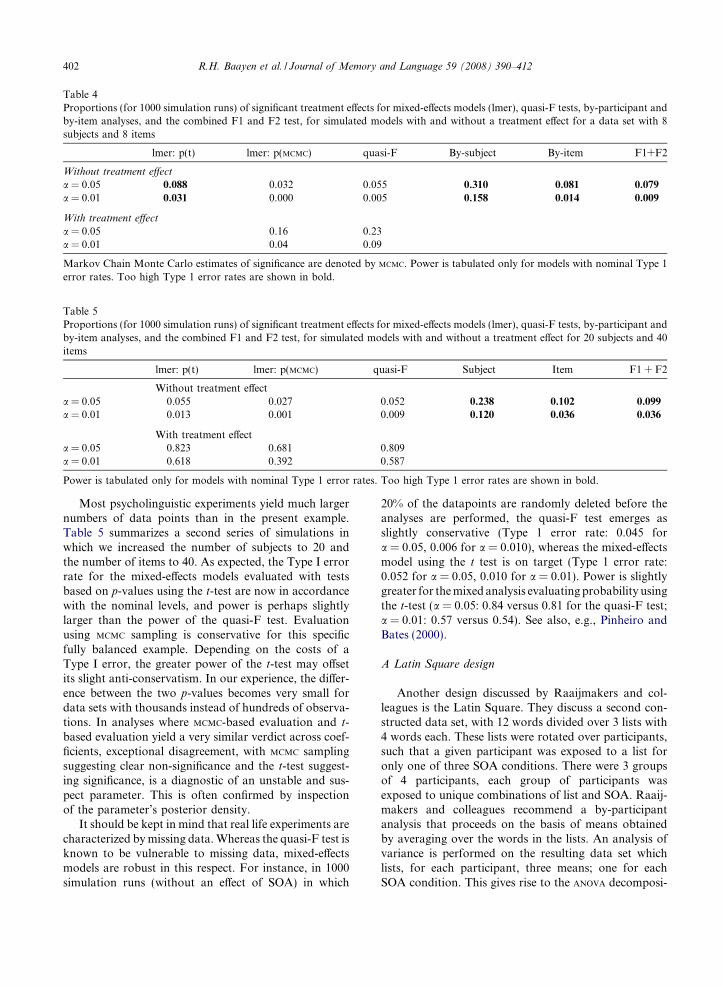
Most psycholinguistic experiments yield much largernumbers of data points than in the present example.Table 5 summarizes a second series of simulations inwhich we increased the number of subjects to 20 andthe number of items to 40. As expected, the Type I errorrate for the mixed-e!ects models evaluated with testsbased on p-values using the t-test are now in accordancewith the nominal levels, and power is perhaps slightlylarger than the power of the quasi-F test. Evaluationusing MCMC sampling is conservative for this specificfully balanced example. Depending on the costs of aType I error, the greater power of the t-test may o!setits slight anti-conservatism. In our experience, the di!er-ence between the two p-values becomes very small fordata sets with thousands instead of hundreds of observa-tions. In analyses where MCMC-based evaluation and t-based evaluation yield a very similar verdict across coef-ficients, exceptional disagreement, with MCMC samplingsuggesting clear non-significance and the t-test suggest-ing significance, is a diagnostic of an unstable and sus-pect parameter. This is often confirmed by inspectionof the parameter’s posterior density.

It should be kept in mind that real life experiments arecharacterized by missing data. Whereas the quasi-F test isknown to be vulnerable to missing data, mixed-e!ectsmodels are robust in this respect. For instance, in 1000simulation runs (without an e!ect of SOA) in which

20% of the datapoints are randomly deleted before theanalyses are performed, the quasi-F test emerges asslightly conservative (Type 1 error rate: 0.045 fora = 0.05, 0.006 for a = 0.010), whereas the mixed-e!ectsmodel using the t test is on target (Type 1 error rate:0.052 for a = 0.05, 0.010 for a = 0.01). Power is slightlygreater for the mixed analysis evaluating probability usingthe t-test (a = 0.05: 0.84 versus 0.81 for the quasi-F test;a = 0.01: 0.57 versus 0.54). See also, e.g., Pinheiro andBates (2000).

A Latin Square design

Another design discussed by Raaijmakers and col-leagues is the Latin Square. They discuss a second con-structed data set, with 12 words divided over 3 lists with4 words each. These lists were rotated over participants,such that a given participant was exposed to a list foronly one of three SOA conditions. There were 3 groupsof 4 participants, each group of participants wasexposed to unique combinations of list and SOA. Raaij-makers and colleagues recommend a by-participantanalysis that proceeds on the basis of means obtainedby averaging over the words in the lists. An analysis ofvariance is performed on the resulting data set whichlists, for each participant, three means; one for eachSOA condition. This gives rise to the ANOVA decomposi-

Table 4Proportions (for 1000 simulation runs) of significant treatment e!ects for mixed-e!ects models (lmer), quasi-F tests, by-participant andby-item analyses, and the combined F1 and F2 test, for simulated models with and without a treatment e!ect for a data set with 8subjects and 8 items

lmer: p(t) lmer: p(MCMC) quasi-F By-subject By-item F1+F2

Without treatment e!ecta = 0.05 0.088 0.032 0.055 0.310 0.081 0.079a = 0.01 0.031 0.000 0.005 0.158 0.014 0.009

With treatment e!ecta = 0.05 0.16 0.23a = 0.01 0.04 0.09

Markov Chain Monte Carlo estimates of significance are denoted by MCMC. Power is tabulated only for models with nominal Type 1error rates. Too high Type 1 error rates are shown in bold.

Table 5Proportions (for 1000 simulation runs) of significant treatment e!ects for mixed-e!ects models (lmer), quasi-F tests, by-participant andby-item analyses, and the combined F1 and F2 test, for simulated models with and without a treatment e!ect for 20 subjects and 40items

lmer: p(t) lmer: p(MCMC) quasi-F Subject Item F1 + F2

Without treatment e!ecta = 0.05 0.055 0.027 0.052 0.238 0.102 0.099a = 0.01 0.013 0.001 0.009 0.120 0.036 0.036

With treatment e!ecta = 0.05 0.823 0.681 0.809a = 0.01 0.618 0.392 0.587

Power is tabulated only for models with nominal Type 1 error rates. Too high Type 1 error rates are shown in bold.


tion shown in Table 6. The F test compares the meansquares for SOA with the mean squares of the interac-tion of SOA by List, and indicates that the e!ect ofSOA is not statistically significant (F(2,2) = 1.15,p = 0.465). As the interaction of SOA by List is not sig-nificant, Raaijmakers et al. (1999) pool the interactionwith the residual error. This results in a pooled errorterm with 20 degrees of freedom, an F-value of 0.896,and a slightly reduced p-value of 0.42.

A mixed-e!ects analysis of the same data set (avail-able as latinsquare in the languageR package)obviates the need for prior averaging. We fit a sequenceof models, decreasing the complexity of the randome!ects structure step by step.

The likelihood ratio tests show that the model with Sub-ject and Word as random e!ects has the right level ofcomplexity for this data set.

>summary(latinsquare.lmer4)Random effects:





(Intercept) 533.9583 13.7098 38.95SOAmedium 2.1250 2.0059 1.06SOAshort %0.4583 2.0059 %0.23

The summary of this model lists the three randome!ects and the corresponding parameters: the variances(and standard deviations) for the random interceptsfor subjects and items, and for the residual error. Thefixed-e!ects part of the model provides estimates forthe intercept and for the contrasts for medium and short

SOA compared to the reference level, long SOA. Inspec-tion of the corresponding p-values shows that thep-value based on the t-test and that based on MCMC sam-pling are very similar, and the same holds for the p-valueproduced by the F-test for the factor SOA

(F(2,141) = 0.944, p = 0.386) and the correspondingp-value calculated from the MCMC samples (p = 0.391).The mixed-e!ects analysis has slightly superior power

> latinsquare.lmer1 = lmer2(RT & SOA + (1jWord) + (1jSubject) + (1jGroup) + (1 + SOA jList),data = latinsquare)> latinsquare.lmer2 = lmer2(RT & SOA + (1jWord) + (1j Subject) + (1jGroup) + (1jList), data =latinsquare)> latinsquare.lmer3 = lmer2(RT& SOA + (1jWord) + (1 jSubject) + (1jGroup), data = latinsquare)> latinsquare.lmer4 = lmer2(RT & SOA + (1jWord) + (1 jSubject), data = latinsquare)> latinsquare.lmer5 = lmer2(RT & SOA + (1jSubject), data = latinsquare)> anova(latinsquare.lmer1, latinsquare.lmer2, latinsquare.lmer3, latinsquare.lmer4,latinsquare.lmer5)


latinsquare.lmer5.p 4 1423.41 1435.29 %707.70latinsquare.lmer4.p 5 1186.82 1201.67 %588.41 238.59 1 <2 e-16latinsquare.lmer3.p 6 1188.82 1206.64 %588.41 0.00 1 1.000latinsquare.lmer2.p 7 1190.82 1211.61 %588.41 1.379e-06 1 0.999latinsquare.lmer1.p 12 1201.11 1236.75 %588.55 0.00 5 1.000

Table 6Mean squares decomposition for the data with a Latin Squaredesign in Raaijmakers et al. (1999)

Df Sum Sq Mean Sq

Group 2 1696 848SOA 2 46 23List 2 3116 1558Group*Subject 9 47305 5256SOA*List 2 40 20Residuals 18 527 29

> pvals.fnc(latinsquare.lmer4, nsim = 10000)


(Intercept) 533.9583 534.0570 503.249 561.828 0.0001 0.0000SOAmedium 2.1250 2.1258 %1.925 5.956 0.2934 0.2912SOAshort %0.4583 %0.4086 %4.331 3.589 0.8446 0.8196


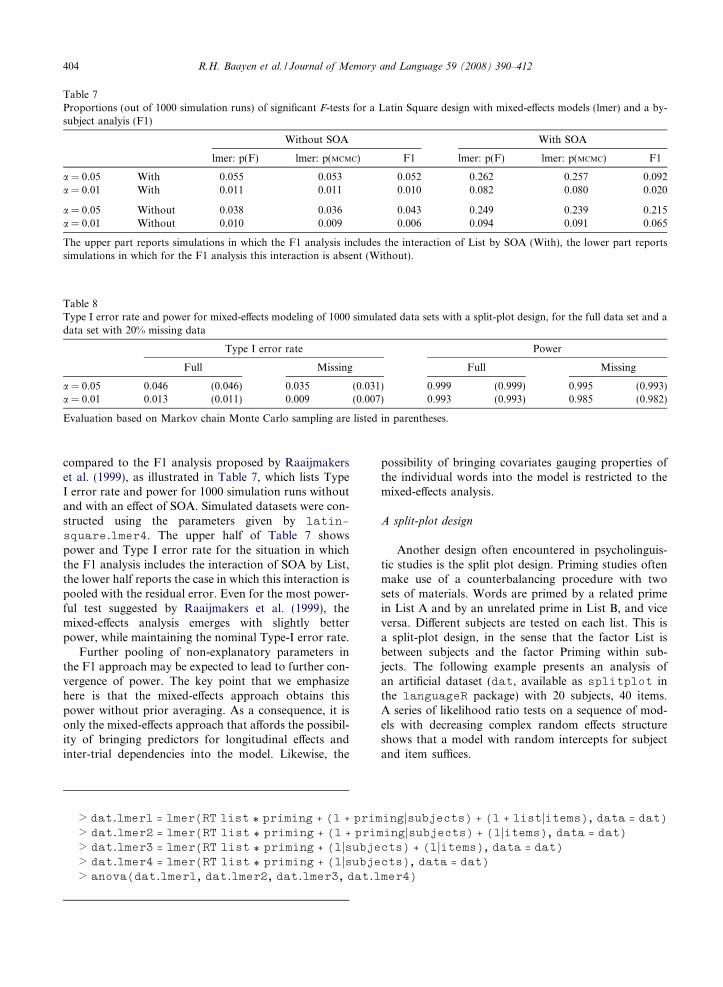
compared to the F1 analysis proposed by Raaijmakerset al. (1999), as illustrated in Table 7, which lists TypeI error rate and power for 1000 simulation runs withoutand with an e!ect of SOA. Simulated datasets were con-structed using the parameters given by latin-square.lmer4. The upper half of Table 7 showspower and Type I error rate for the situation in whichthe F1 analysis includes the interaction of SOA by List,the lower half reports the case in which this interaction ispooled with the residual error. Even for the most power-ful test suggested by Raaijmakers et al. (1999), themixed-e!ects analysis emerges with slightly betterpower, while maintaining the nominal Type-I error rate.

Further pooling of non-explanatory parameters inthe F1 approach may be expected to lead to further con-vergence of power. The key point that we emphasizehere is that the mixed-e!ects approach obtains thispower without prior averaging. As a consequence, it isonly the mixed-e!ects approach that a!ords the possibil-ity of bringing predictors for longitudinal e!ects andinter-trial dependencies into the model. Likewise, the

possibility of bringing covariates gauging properties ofthe individual words into the model is restricted to themixed-e!ects analysis.

A split-plot design

Another design often encountered in psycholinguis-tic studies is the split plot design. Priming studies oftenmake use of a counterbalancing procedure with twosets of materials. Words are primed by a related primein List A and by an unrelated prime in List B, and viceversa. Di!erent subjects are tested on each list. This isa split-plot design, in the sense that the factor List isbetween subjects and the factor Priming within sub-jects. The following example presents an analysis ofan artificial dataset (dat, available as splitplot inthe languageR package) with 20 subjects, 40 items.A series of likelihood ratio tests on a sequence of mod-els with decreasing complex random e!ects structureshows that a model with random intercepts for subjectand item su#ces.

Table 7Proportions (out of 1000 simulation runs) of significant F-tests for a Latin Square design with mixed-e!ects models (lmer) and a by-subject analyis (F1)

Without SOA With SOA

lmer: p(F) lmer: p(MCMC) F1 lmer: p(F) lmer: p(MCMC) F1

a = 0.05 With 0.055 0.053 0.052 0.262 0.257 0.092a = 0.01 With 0.011 0.011 0.010 0.082 0.080 0.020

a = 0.05 Without 0.038 0.036 0.043 0.249 0.239 0.215a = 0.01 Without 0.010 0.009 0.006 0.094 0.091 0.065

The upper part reports simulations in which the F1 analysis includes the interaction of List by SOA (With), the lower part reportssimulations in which for the F1 analysis this interaction is absent (Without).

> dat.lmer1 = lmer(RT list * priming + (1 + primingjsubjects) + (1 + listjitems), data = dat)> dat.lmer2 = lmer(RT list * priming + (1 + primingjsubjects) + (1jitems), data = dat)> dat.lmer3 = lmer(RT list * priming + (1jsubjects) + (1jitems), data = dat)> dat.lmer4 = lmer(RT list * priming + (1jsubjects), data = dat)> anova(dat.lmer1, dat.lmer2, dat.lmer3, dat.lmer4)

Table 8Type I error rate and power for mixed-e!ects modeling of 1000 simulated data sets with a split-plot design, for the full data set and adata set with 20% missing data

Type I error rate Power

Full Missing Full Missing

a = 0.05 0.046 (0.046) 0.035 (0.031) 0.999 (0.999) 0.995 (0.993)a = 0.01 0.013 (0.011) 0.009 (0.007) 0.993 (0.993) 0.985 (0.982)

Evaluation based on Markov chain Monte Carlo sampling are listed in parentheses.


The estimates are close to the parameters that generatedthe simulated data: ri = 20, rs = 50, r = 80, bint = 400,bpriming = 30, blist = 18.5, blist:priming = 0.

Table 8 lists power and Type I error rate with respect tothe priming e!ect for 1000 simulation runs with a mixed-e!ect model, run once with the full data set, and once with20% of the data points randomly deleted, using the sameparameters that generated the above data set. It is clearthat with the low level of by-observation noise, the pres-ence of a priming e!ect is almost always detected. Powerdecreases only slightly for the case with missing data. Eventhough power is at ceiling, the Type I error rate is in accor-dance with the nominal levels. Note the similarity betweenevaluation of significance based on the (anticonservative)t-test and evaluation based on Markov chain Monte Car-lo sampling. This example illustrates the robustness ofmixed e!ects models with respect to missing data: Thepresent results were obtained without any data pruningand without any form of imputation.

A multiple regression design

Multiple regression designs with subjects and items,and with predictors that are tied to the items (e.g., fre-quency and length for items that are words) have tradi-tionally been analyzed in two ways. One approachaggregates over subjects to obtain item means, and thenproceeds with standard ordinary least squares regression.We refer to this as by-item regression. Another approach,advocated by Lorch and Myers (1990), is to fit separateregression models to the data sets elicited from the indi-vidual participants. The significance of a given predictor

is assessed by means of a one-sample t-test applied tothe coe#cients of this predictor in the individual regres-sion models. We refer to this procedure as by-participantregression. It is also known under the name of randomregression. (From our perspective, these procedures com-bine precise and imprecise information on an equal foot-ing.) Some studies report both by-item and by-participantregression models (e.g., Alegre & Gordon, 1999).

The by-participant regression is widely regarded assuperior to the by-item regression. However, the by-par-ticipant regression does not take item-variability intoaccount. To see this, compare an experiment in whicheach participant responds to the same set of words to anexperiment in which each participant responds to a di!er-ent set of words. When the same lexical predictors are usedin both experiments, the by-participant analysis proceedsin exactly the same way for both. But whereas thisapproach is correct for the second experiment, it ignoresa systematic source of variation in the case of the firstexperiment.

A simulation study illustrates that ignoring item var-iability that is actually present in the data may lead tounacceptably high Type I error rates. In this simulationstudy, we considered three predictors, X, Y and Z tied to20 items, each of which was presented to 10 participants.In one set of simulation runs, these predictors had betaweights 2, 6 and 4. In a second set of simulation runs,the beta weight for Z was set to zero. We were interestedin the power and Type I error rates for Z for by-partic-ipant and for by-item regression, and for two di!erentmixed-e!ects models. The first mixed-e!ects model thatwe considered included crossed random e!ects for par-


dat.lmer4.p 5 9429.0 9452.4 %4709.5dat.lmer3.p 6 9415.0 9443.1 %4701.5 15.9912 1 6.364e-05dat.lmer2.p 8 9418.8 9456.3 %4701.4 0.1190 2 0.9423dat.lmer1.p 10 9419.5 9466.3 %4699.7 3.3912 2 0.1835

> print(dat.lmer3, corr = FALSE)Random effects:


items (Intercept) 447.15 21.146subjects (Intercept) 2123.82 46.085Residual 6729.24 82.032

Number of obs: 800, groups: items, 40; subjects, 20Fixed effects:

Estimate Std. Error t value(Intercept) 362.658 16.382 22.137listlistB 18.243 23.168 0.787primingunprimed 31.975 10.583 3.021listlistB:primingunprimed

%6.318 17.704 %0.357


ticipant and item with random intercepts only. Thismodel reflected exactly the structure implemented inthe simulated data. A second mixed-e!ects modelignored the item structure in the data, and included onlyparticipant as a random e!ect. This model is the mixed-e!ects analogue to the by-participant regression.

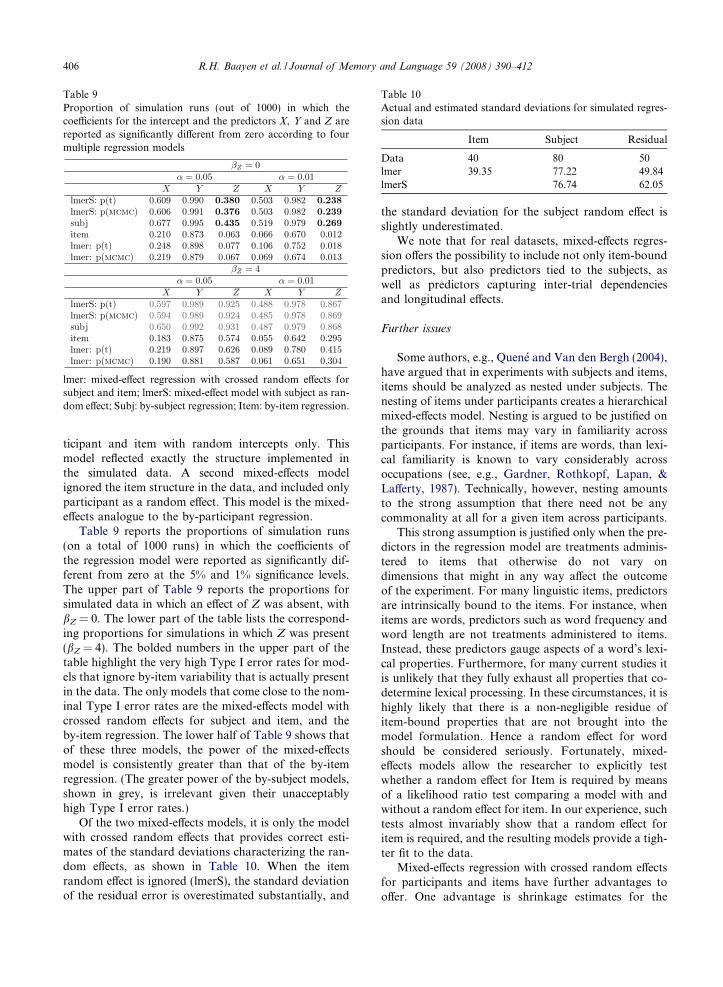
Table 9 reports the proportions of simulation runs(on a total of 1000 runs) in which the coe#cients ofthe regression model were reported as significantly dif-ferent from zero at the 5% and 1% significance levels.The upper part of Table 9 reports the proportions forsimulated data in which an e!ect of Z was absent, withbZ = 0. The lower part of the table lists the correspond-ing proportions for simulations in which Z was present(bZ = 4). The bolded numbers in the upper part of thetable highlight the very high Type I error rates for mod-els that ignore by-item variability that is actually presentin the data. The only models that come close to the nom-inal Type I error rates are the mixed-e!ects model withcrossed random e!ects for subject and item, and theby-item regression. The lower half of Table 9 shows thatof these three models, the power of the mixed-e!ectsmodel is consistently greater than that of the by-itemregression. (The greater power of the by-subject models,shown in grey, is irrelevant given their unacceptablyhigh Type I error rates.)

Of the two mixed-e!ects models, it is only the modelwith crossed random e!ects that provides correct esti-mates of the standard deviations characterizing the ran-dom e!ects, as shown in Table 10. When the itemrandom e!ect is ignored (lmerS), the standard deviationof the residual error is overestimated substantially, and

the standard deviation for the subject random e!ect isslightly underestimated.

We note that for real datasets, mixed-e!ects regres-sion o!ers the possibility to include not only item-boundpredictors, but also predictors tied to the subjects, aswell as predictors capturing inter-trial dependenciesand longitudinal e!ects.

Further issues

Some authors, e.g., Quene and Van den Bergh (2004),have argued that in experiments with subjects and items,items should be analyzed as nested under subjects. Thenesting of items under participants creates a hierarchicalmixed-e!ects model. Nesting is argued to be justified onthe grounds that items may vary in familiarity acrossparticipants. For instance, if items are words, than lexi-cal familiarity is known to vary considerably acrossoccupations (see, e.g., Gardner, Rothkopf, Lapan, &La!erty, 1987). Technically, however, nesting amountsto the strong assumption that there need not be anycommonality at all for a given item across participants.

This strong assumption is justified only when the pre-dictors in the regression model are treatments adminis-tered to items that otherwise do not vary ondimensions that might in any way a!ect the outcomeof the experiment. For many linguistic items, predictorsare intrinsically bound to the items. For instance, whenitems are words, predictors such as word frequency andword length are not treatments administered to items.Instead, these predictors gauge aspects of a word’s lexi-cal properties. Furthermore, for many current studies itis unlikely that they fully exhaust all properties that co-determine lexical processing. In these circumstances, it ishighly likely that there is a non-negligible residue ofitem-bound properties that are not brought into themodel formulation. Hence a random e!ect for wordshould be considered seriously. Fortunately, mixed-e!ects models allow the researcher to explicitly testwhether a random e!ect for Item is required by meansof a likelihood ratio test comparing a model with andwithout a random e!ect for item. In our experience, suchtests almost invariably show that a random e!ect foritem is required, and the resulting models provide a tigh-ter fit to the data.

Mixed-e!ects regression with crossed random e!ectsfor participants and items have further advantages too!er. One advantage is shrinkage estimates for the

Table 9Proportion of simulation runs (out of 1000) in which thecoe#cients for the intercept and the predictors X, Y and Z arereported as significantly di!erent from zero according to fourmultiple regression models

lmer: mixed-e!ect regression with crossed random e!ects forsubject and item; lmerS: mixed-e!ect model with subject as ran-dom e!ect; Subj: by-subject regression; Item: by-item regression.

Table 10Actual and estimated standard deviations for simulated regres-sion data

Item Subject Residual

Data 40 80 50lmer 39.35 77.22 49.84lmerS 76.74 62.05


BLUPs (the subject and item specific adjustments to inter-cepts and slopes), which allow enhanced prediction forthese items and subjects (see, e.g., Baayen, 2008, for fur-ther discussion). Another important advantage is thepossibility to include simultaneously predictors thatare tied to the items (e.g., frequency, length) and predic-tors that are tied to participants (e.g., handedness, age,gender). Mixed-e!ects models have also been extendedto generalized linear models and can hence be used e#-ciently to model binary response data such as accuracyin lexical decision (see Jaeger, this volume).

To conclude, we briefly address the question of theextent to which an e!ect observed to be significant in amixed-e!ects analysis generalizes across both subjectsand items (see Forster, this issue). The traditional inter-pretation of the F1 (by-subject) and F2 (by-item) analy-ses is that significance in the F1 analysis would indicatethat the e!ect is significant for all subjects, and that theF2 analysis would indicate that the e!ect holds for allitems. We believe this interpretation is incorrect. In fact,even if we replace the F1+F2 procedure by a mixed-e!ects model, the inference that the e!ect would general-ize across all subjects and items remains incorrect. Thefixed-e!ect coe#cients in a mixed-e!ect model are esti-mates of the intercept, slopes (for numeric predictors)or contrasts (for factors) in the population for the aver-age, unknown subject and the average, unknown item.Individual subjects and items may have intercepts andslopes that diverge considerably from the populationmeans. For ease of exposition, we distinguish three pos-sible states of a!airs for what in the traditional terminol-ogy would by described as an E!ect by Item interaction.

First, it is conceivable that the BLUPs for a given fixed-e!ect coe#cient, when added to that coe#cient, neverchange its sign. In this situation, the e!ect indeed gener-alizes across all subjects (or items) sampled in the exper-iment. Other things being equal, the partial e!ect of thepredictor quantified by this coe#cient will be highlysignificant.

Second, situations arise in which adding the BLUPs toa fixed coe#cient results in a majority of by-subject (orby-item) coe#cients that have the same sign as the pop-ulation estimate, in combination with a relatively smallminority of by-subject (or by-item) coe#cients with theopposite sign. The partial e!ect represented by the pop-ulation coe#cient will still be significant, but there willbe less reason for surprise. The e!ect generalizes to amajority, but not to all subjects or items. Nevertheless,we can be confident about the magnitude and sign ofthe e!ect on average, for unknown subjects or items, ifthe subjects and items are representative of the popula-tion from which they are sampled.

Third, the by-subject (or by-item) coe#cientsobtained by taking the BLUPs into account may resultin a set of coe#cients with roughly equal numbers ofcoe#cients that are positive and coe#cients that are

negative. In this situation, the main e!ect (for a numericpredictor or a binary contrast) will not be significant, incontradistinction to the significance of the random e!ectfor the slopes or contrasts at issue. In this situation,there is a real and potentially important e!ect, but aver-aged across subjects or items, it cancels out to zero.

In the field of memory and language, experimentsthat do not yield a significant main e!ect are generallyconsidered to have failed. However, an experimentresulting in this third state of a!airs may constitute apositive step forward for our understanding of languageand language processing. Consider, by way of example,a pharmaceutical company developing a new medicine,and suppose this medicine has adverse side e!ects forsome, but highly beneficial e!ects for other patients—patients for which it is an e!ective life-saver. The com-pany could decide not to market the medicine becausethere is no main e!ect. However, they can actually makesubstantial profit by bringing it on the market withwarnings for adverse side e!ects and proper distribu-tional controls.

Returning to our own field, we know that no twobrains are the same, and that di!erent brains have di!er-ent developmental histories. Although in the initialstages of research the available technology may onlyreveal the most robust main e!ects, the more ourresearch advances, the more likely it will become thatwe will be able to observe systematic individual di!er-ences. Ultimately, we will need to bring these individualdi!erences into our theories. Mixed-e!ect models havebeen developed to capture individual di!erences in aprincipled way, while at the same time allowing general-izations across populations. Instead of discarding indi-vidual di!erences across subjects and items as anuninteresting and disappointing nuisance, we shouldembrace them. It is not to the advantage of scientificprogress if systematic variation is systematically ignored.

Hierarchical models in developmental and educationalpsychology

Thus far, we have focussed on designs with crossedrandom e!ects for subjects and items. In educationaland developmental research, designs with nested ran-dom e!ects are often used, such as the natural hierarchyformed by students nested within a classroom (Gold-stein, 1987). Such designs can also be handled bymixed-e!ects models, which are then often referred toas hierarchical linear models or multilevel models.

Studies in educational settings are often focused onlearning over time, and techniques developed for thistype of data often attempt to characterize how individu-als’ performance or knowledge changes over time,termed the analysis of growth curves (Goldstein, 1987,1995; Goldstein et al., 1993; Nutall, Goldstein, Prosser,


& Rasbash, 1989; Willet, Singer, & Martin, 1998).Examples of this include the assessment of di!erentteaching techniques on students performance (Aitkin,Anderson, & Hinde, 1981), and the comparison of thee!ectiveness of di!erent schools (Aitkin & Longford,1986). Goldstein et al. (1993) used multilevel techniquesto study the di!erences between schools and studentswhen adjusting for pre-existing di!erences when studentsentered classes. For a methodological discussion of theuse of these models, see the collection of articles in theSummer 1995 special issue of Journal of Educational andBehavioral Statistics on hierarchical linear models, e.g.,Kreft (1995). Singer (1998) provides a practical introduc-tion to multilevel models including demonstration code,and Collins (2006) provides a recent overview of issuesin longitudinal data analysis involving these models.Finally, Fielding and Goldstein (2006) provide a compre-hensive overview of multilevel and cross-classified modelsapplied to education research, including a brief softwarereview. West et al. (2007) provide a comprehensive soft-ware review for nested mixed-e!ects models.

These types of models are also applicable to psycho-linguistic research, especially in studies of developmentalchange. Individual speakers from a language communityare often members of a hierarchy, e.g., language:dia-lect:family:speaker, and many studies focus on learningor language acquisition, and thus analysis of change ordevelopment is important. Huttenlocher, Haight, Bryk,and Seltzer (1991) used multilevel models to assess theinfluence of parental or caregiver speech on vocabularygrowth, for example. Boyle and Willms (2001) providean introduction to the use of multilevel models to studydevelopmental change, with an emphasis on growthcurve modeling and discrete outcomes. Raudenbush(2001) reviews techniques for analyzing longitudinaldesigns in which repeated measures are used. Recently,Misangyi, LePine, Algina, and Goeddeke (2006) com-pared repeated measures regression to multivariateANOVA (MANOVA) and multilevel analysis in researchdesigns typical for organizational and behavioralresearch, and concluded that multilevel analysis can pro-vide equivalent results as MANOVA, and in cases wherespecific assumptions about variance-covariance struc-tures could be made, or in cases where missing valueswere present, that multilevel modeling is a better analy-sis strategy and in some cases a necessary strategy (seealso Kreft & de Leeuw, 1998 and Snijders & Bosker,1999).

Finally, a vast body of work in educational psychol-ogy concerns test construction and the selection of testitems (Lord & Novick, 1968). Although it is beyondthe scope of this article to review this work, it shouldbe noted that work within generalizability theory (Cron-bach, Gleser, Nanda, & Rajaratnam, 1972) has beenconcerned with the problem of crossed subject and itemfactors using random e!ects models (Schroeder & Haks-

tian, 1990). For a recent application of the software con-sidered here to item response theory, see Doran, Bates,Bliese, and Dowling (2007), and for the application ofhierarchical models to joint response type and responsetime measures, see Fox, Entink, and van der Linden(2007).

Mixed-e!ects models in neuroimaging

In neuroimaging, two-level or mixed e!ects modelsare now a standard analysis technique (Friston et al.,2002a, 2002b; Worsley et al., 2002), and are used in con-junction with Gaussian Random Field theory to makeinferences about activity patterns in very large data sets(voxels from fMRI scans). These techniques are formallycomparable to the techniques that are advocated in thispaper (Friston, Stephan, Lund, Morcom, & Kiebel,2005). Interestingly, however, the treatment of stimulias random e!ects has not been widely addressed in theimaging and physiological community, until recently(Bedny, Aguirre, & Thompson-Schill, 2007).

In imaging studies that compare experimental condi-tions, for example, statistical parameter maps (SPM; Fris-ton et al., 1995) are calculated based on successivelyrecorded time series for the di!erent experimental condi-tions. A hypothesized hemodynamic response functionis convolved with a function that encodes the experimen-tal design matrix, and this forms a regressor for each ofthe time series in each voxel. Significant parameters forthe regressors are taken as evidence of activity in thevoxels that exhibit greater or less activity than isexpected based on the null hypothesis of no activity dif-ference between conditions. The logic behind these testsis that a rejection of the null hypothesis for a region isevidence for a di!erence in activity in that region.

Neuroimaging designs are often similar to cognitivepsychology designs, but the dimension of the responsevariable is much larger and the nature of the responsehas di!erent statistical properties. However, this is notcrucial for the application of mixed e!ects models. Infact, it shows the technique can scale to problems thatinvolve very large datasets.

A prototypical case of a fixed e!ects analysis in fMRIwould test whether a image contrast is statistically sig-nificant within a single subject over trials. This wouldbe analogous to a psychophysics experiment using onlya few participants, or a patient case study. For randome!ect analysis the parameters calculated from the singleparticipants are used in a mixed model to test whether acontrast is significant over participants, in order to testwhether the contrasts reflects a di!erence in the popula-tion from which the participants were sampled. This isanalogous to how cognitive psychology experimenterstreat mean RTs, for example. A common analysis strat-egy is to calculate a single parameter for each participant


in an RT study, and then analyze this data in (what inthe neuroimaging community is called) a random e!ectsanalysis.

The estimation methods used to calculate the statisti-cal parameters of these models include Maximum Like-lihood or Restricted Maximum Likelihood, just as in theapplication of the multilevel models used in educationresearch described earlier. One reason that these tech-niques are used is to account for correlation betweensuccessive measurements in the imaging time series.These corrections are similar to corrections familiar topsychologists for non-sphericity (Greenhouse & Geisser,1958).

Similar analysis concerns are present within electro-physiology. In the past, journal policy in psychophysio-logical research has dealt with the problems posed byrepeated measures experimental designs by suggestingthat researchers adopt statistical procedures that takeinto account the correlated data obtained from thesedesigns (Jennings, 1987; Vasey & Thayer, 1987). Mixede!ects models are less commonly applied in psychophys-iological research, as the most common techniques arethe traditional univariate ANOVA with adjustments ormultivariate ANOVA (Dien & Santuzzi, 2004), but someresearchers have advocated them to deal with repeatedmeasures data. For example, Bagiella, Sloan, and Heit-jan (2000) suggest that mixed e!ects models have advan-tages over more traditional techniques for EEG dataanalysis.

The current practice of psychophysiologists and neu-roimaging researchers typically ignores the issue ofwhether linguistic materials should be modeled withfixed or random e!ect models. Thus, while there aretechniques available for modeling stimuli as randome!ects, it is not yet current practice in neuroimagingand psychophysiology to do so. This represents a tre-mendous opportunity for methodological developmentin language-related imaging experiments, as psycholin-guists have considerable experience in modeling stimuluscharacteristics.

Cognitive psychologists and neuroscientists mightreasonably assume that the language-as-a-fixed-e!ectdebate is only a concern when linguistic materials areused, given that most discussion to date has taken placein the context of linguistically-motivated experiments.This assumption is too narrow, however, because natu-ralistic stimuli from many domains are drawn frompopulations.

Consider a researcher interested in the electrophysiol-ogy of face perception. She designs an experiment to testwhether an ERP component such as the N170 in responseto faces has a di!erent amplitude in one of two face con-ditions, normal and scrambled form. She obtains a set ofimages from a database, arranges them according to herexperimental design, and proceeds to present each pic-ture in a face-detection EEG experiment, analogous to

the way that a psycholinguist would present words andnon-words to a participant in a lexical decision experi-ment. The images presented in this experiment wouldbe a sample of all possible human faces. It is not contro-versial that human participants are to be modeled as arandom variable in psychological experiments. Picturesof human faces are images of a random variable, pre-sented as stimuli. Thus, it should be no source of contro-versy that naturalistic face stimuli are also a randomvariable, and should be modeled as a random e!ect, justlike participants. For the sake of consistency, if humanparticipants, faces, and speech are to be considered ran-dom variables, then objects, artifacts, and scenes mightjust as well be considered random variables (also pointedout by Raaijmakers, 2003).

Any naturalistic stimulus which is a member of apopulation of stimuli which has not been exhaustivelysampled should be considered a random variable forthe purposes of an experiment. Note that random in thissense means STOCHASTIC, a variable subject to probabilis-tic variation, rather than randomly sampled. A randomsample is one method to draw samples from a popula-tion and assign them to experimental condition. How-ever, stimuli may have stochastic characteristicswhether or not they are randomly sampled or not. Par-ticipants have stochastic characteristics, as well, whetherthey are randomly sampled or not. Therefore, the pres-ent debate about the best way to model random e!ectsof stimuli is wider than previously has been appreciated,and should be seen as part of the debate over the use ofnaturalistic stimuli in sensory neurophysiology as well(Felsen & Yang, 2005; Ruse & Movshon, 2005).

Concluding remarks

We have described the advantages that mixed-e!ectsmodels with crossed random e!ects for subject and itemo!er to the analysis of experimental data.

The most important advantage of mixed-e!ects mod-els is that they allow the researcher to simultaneouslyconsider all factors that potentially contribute to theunderstanding of the structure of the data. These factorscomprise not only standard fixed-e!ects factors typicallymanipulated in psycholinguistic experiments, but alsocovariates bound to the items (e.g., frequency, complex-ity) and the subjects (e.g., age, sex). Furthermore, localdependencies between the successive trials in an experi-ment can be brought into the model, and the e!ects ofprior exposure to related or identical stimuli (as inlong-distance priming) can be taken into account aswell. (For applications in eye-movement research, seeKliegl, 2007, and Kliegl, Risse, & Laubrock, 2007).Mixed-e!ects models may o!er substantially enhancedinsight into how subjects are performing in the courseof an experiment, for instance, whether they are adjust-


ing their behavior as the experiment proceeds to opti-mize performance. Procedures requiring prior averagingacross subjects or items, or procedures that are limitedto strictly factorial designs, cannot provide theresearcher with the analytical depth typically providedby a mixed-e!ects analysis.

For data with not too small numbers of observations,mixed-e!ects models may provide modest enhancedpower, as illustrated for a Latin Square design in thepresent study. For regression and analysis of covariance,mixed-e!ects modeling protects against inflated signifi-cance for data sets with significant by-item randome!ects structure. Other advantages of mixed-e!ects mod-eling that we have mentioned only in passing are theprincipled way in which non-independence (asphericity)is handled through the variance-covariance structure ofthe model, and the provision of shrinkage estimatesfor the by-subject and by-item adjustments to interceptand slopes, which allows enhanced precision inprediction.

An important property of mixed-e!ects modeling isthat it is possible to fit models to large, unbalanced datasets. This allows researchers to investigate not only dataelicited under controlled experimental conditions, but toalso study naturalistic data, such as corpora of eye-movement data. Markov chain Monte Carlo samplingfrom the posterior distribution of the parameters is ane#cient technique to evaluate fitted models with respectto the stability of their parameters and to distinguishbetween robust parameters (with narrow highest poster-ior density intervals) from superfluous parameters (withvery broad density intervals).

Mixed-e!ects modeling is a highly active researchfield. Well-established algorithms and techniques forparameter estimation are now widely available. Onequestion that is still hotly debated is the appropriatenumber of degrees of freedom for the fixed-e!ects fac-tors. Di!erent software packages make use of or eveno!er di!erent choices. We have emphasized the impor-tance of Markov chain Monte Carlo sampling as fastand e#cient way (compared to, e.g., the bootstrap) toevaluate a model’s parameters. In our experience, p-val-ues based on MCMC sampling and p-values based onthe upper bound of the degrees of freedom tend to bevery similar for all but the smallest samples.

An important goal driving the development of thelme4 package in R, the software that we have intro-duced and advocated here, is to make it possible to dealrealistically with the parameters of models fit to large,unbalanced data sets. Bates (2007a) provides an exampleof a data set with about 1.7 million observations, 55000‘‘subjects” (distinct students at a major university over a5 year period) and 7900 ‘‘items” (instructors). The dataare unbalanced and the subject and item factors are par-tially crossed. Fitting a simple model with randome!ects for subject and for item took only about an hour

on a fast server computer with substantial memory.Thanks to the possibility of handling very large datasets, we anticipate mixed-e!ects modeling to becomeincreasingly important for improved modeling of spatialand temporal dependencies in neuroimaging studies, aswell as for the study of naturalistic corpus-based datain chronometric tasks and eye-movement research. Inshort, mixed-e!ects modeling is emerging not only as auseful but also as an actually useable tool for comingto a comprehensive understanding of the quantitativestructure of highly complex data sets.

A note on parameter estimation

The mathematical details of model fitting with mixed e!ectsmodels are beyond the scope of the present paper (see Bates,2007, for an introduction), we note here that fitting the modelinvolves finding the right balance between the complexity ofthe model and faithfulness to the data. Model complexity isdetermined primarily by the parameters that we invest in therandom e!ects structure, basically the parameters that definethe relative variance-covariance matrix R in Eq. (10). Interest-ingly, the profiled deviance function, which is negative twicethe log-likelihood of model (10) evaluated at R, b and r2 fora given set of parameters, can be estimated without having tosolve for b or b. The profiled deviance function has two compo-nents, one that measures model complexity and one that mea-sures fidelity of the fitted values to the observed data. This isillustrated in Fig. 2.

Each panel has the relative standard deviation of the itemrandom e!ect (i.e., ri/r) on the horizontal axis, and the relativestandard deviation of the subject random e!ect (rs/r) on thevertical axis. First consider the rightmost panel. As we allowthese two relative standard deviations to increase, the fidelityto the data increases and the deviance (the logarithm of thepenalized residual sum of squares) decreases. In the contourplot, darker shades of grey represent greater fidelity anddecreased deviance, and it is easy to see that a better fit isobtained for higher values for the item and subject relative stan-dard deviations. However, increasing these relative standarddeviations leads to a model that is more complex.2 This isshown in the middle panel, which plots the contours of themodel complexity, the logarithm of the determinant of a matrixderived from the random e!ects matrix Z. Darker shades ofgrey are now found in the lower left corner, instead of in theupper right corner. The left panel of Fig. 2 shows the compro-mise between model complexity and fidelity to the data in theform of the deviance function that is minimized at the maxi-

2 The relation between model complexity and the magnitudesof the item and subject relative standard deviations is mosteasily appreciated by considering the limiting case in whichboth relative standard deviations are zero. These two param-eters can now be removed from the symbolic specification of themodel. This reduction in the number of parameters is thefamiliar index of model simplification.


mum likelihood estimates. The + symbols in each panel denotethe values of the deviance components at the maximum likeli-hood estimates.

References

Aitkin, M., Anderson, D., & Hinde, J. (1981). Statisticalmodeling of data on teaching styles. Journal of the RoyalStatistical Society, A, 144, 148–161.

Aitkin, M., & Longford, N. (1986). Statistical modeling inschool e!ectiveness studies. Journal of the Royal StatisticalSociety, A, 149, 1–43.

Alegre, M., & Gordon, P. (1999). Frequency e!ects and therepresentational status of regular inflections. Journal ofMemory and Language, 40, 41–61.

Andrieu, C., de Freitas, N., Doucet, A., & Jordan, M. I. (2003).An introduction to MCMC for machine learning. MachineLearning, 50, 5–43.

Baayen, R. H. (2008). Analyzing linguistic data: A practicalintroduction to statistics. Cambridge: Cambridge UniversityPress.

Bagiella, E., Sloan, R. P., & Heitjan, D. F. (2000). Mixed-e!ectsmodels in psychophysiology. Psychophysiology, 37, 13–20.

Bates, D. M., & Sarkar, D. (2007). lme4: Linear mixed-e!ectsmodels using S4 classes, R package version 0.99875-6.

Bates, D. M. (2005). Fitting linear mixed models in R. R News,5, 27–30.

Bates, D. M. (2007). Linear mixed model implementation inlme4. Manuscript, university of Wisconsin - Madison,January 2007.

Bates, D. M. (2007a). Fitting linear, generalized linear and mixedmodels to large data sets. Paper presented at useR!2007,Ames, Iowa, August 2007.

Bedny, M., Aguirre, G. K., & Thompson-Schill, S. L. (2007).Item analysis in functional magnetic resonance imaging.Neuroimage, 35, 1093–1102.

Boyle, M. H., & Willms, J. D. (2001). Multilevel modeling ofhierarchical data in developmental studies. Journal of Child

Psychology and Psychiatry and Allied Disciplines, 42,141–162.

Box, G. E. P., & Tiao, G. C. (1992). Bayesian inference instatistical analysis. New York: Wiley.

Clark, H. H. (1973). The language-as-fixed-e!ect fallacy: Acritique of language statistics in psychological research.Journal of Verbal Learning and Verbal Behavior, 12,335–359.

Coleman, E. B. (1964). Generalizing to a language population.Psychological Reports, 14, 219–226.

Collins, L. M. (2006). Analysis of longitudinal data: Theintegration of theoretical models, design, and statisticalmodel. Annual Review of Psychology, 57, 505–528.

Cronbach, L. J., Gleser, G. C., Nanda, H., & Rajaratnam, N.(1972). The dependability of behavioral measurements. NewYork: Wiley.

Dien, J., & Santuzzi, A. M. (2004). Application of repeatedmeasures ANOVA to high-density ERP datasets: A review andtutorial. In T. Handy (Ed.), Event-related potentials. Cam-bridge: MIT Press.

Doran, H., Bates, D., Bliese, P., & Dowling, M. (2007).Estimating the multilevel Rasch model with the lme4package. Journal of Statistical Software, 20, 1–18.

Faraway, J. J. (2006). Extending the linear model with R. BocaRaton, FL: Chapman & Hall/CRC.

Felsen, G., & Yang, D. (2005). A natural approach to studyingvision. Nature Neuroscience, 8, 1643–1646.

Fielding, A., & Goldstein, H. (2006). Cross-classified andmultiple membership structures in multilevel models: Anintroduction and review. Research Report No. 791. Depart-ment of Eduction and Skills. University of Birmingham.ISBN 1 84478797 2.

Forster, K. I., & Dickinson, R. G. (1976). More on thelanguage-as-fixed e!ect: Monte-Carlo estimates of errorrates for F1, F2, F0, and minF0. Journal of Verbal Learningand Verbal Behavior, 15, 135–142.

Fox, J., Entink, R., & van der Linden, W. (2007). Modeling ofresponses and response times with the package CIRT. Journalof Statistical Software, 20, 1–14.

""1

"" 2

1

2

3

4

1 2 3 4

155156

157

158

158159

59

160

161

161

162

162

163

163

164

164

165

165

166

1616

deviance

1 2 3 4

6 810

1214

16

18

20

22

24

model complexity

1 2 3 4

7.6

7.88.08.28.48.6

fidelity

Fig. 2. Contours of the profiled deviance as a function of the relative standard deviations of the item random e!ects (x-axis) and thesubject random e!ects (y-axis). The leftmost panel shows the deviance, the function that is minimized at the maximum likelihoodestimates, the middle panel shows the component of the deviance that measures model complexity and the rightmost panel shows thecomponent of the deviance that measures fidelity of the fitted values to the observed data.


Friston, K. J., Glaser, D. E., Henson, R. N. A., Kiebel, S.,Phillips, C., & Ashburner, J. (2002a). Classical and Bayesianinference in neuroimaging: Applications. NeuroImage, 16,484–512.

Friston, K. J., Holmes, A. P., Worsley, K. J., Poline, J.-B., Frith, C. D., & Frackowiak, R. S. J. (1995).Statistical parametric maps in functional imaging: Ageneral linear approach. Human Brain Mapping, 2,189–210.

Friston, K. J., Penny, W., Phillips, C., Kiebel, S., Hinton, G., &Ashburner, J. (2002b). Classical and Bayesian inference inneuroimaging: Theory. NeuroImage, 16, 465–483.

Friston, K. J., Stephan, K. E., Lund, T. E., Morcom, A., &Kiebel, S. (2005). Mixed-e!ects and fMRI studies. Neuro-Image, 24, 244aAS!–252aAS!.

Gardner, M. K., Rothkopf, E. Z., Lapan, R., & La!erty, T.(1987). The word frequency e!ect in lexical decision:Finding a frequency-based component. Memory and Cog-nition, 15, 24–28.

Gilmour, A. R., Thompson, R., & Cullis, B. R. (1995). AI, ane#cient algorithm for REML estimation in linear mixedmodels. Biometrics, 51, 1440–1450.

Gilmour, A. R., Gogel, B. J., Cullis, B. R., Welham, S. J., &Thompson, R. (2002). ASReml User Guide Release 1.0. VSNInternational, 5 The Waterhouse, Waterhouse St, HemelHempstead, HP1 1ES, UK.

Goldstein, H. (1987). Multilevel models in educational and socialresearch. London: Gri#n.

Goldstein, H., Rasbash, J., Yang, M., Woodhouse, G., Pan, H.,Nuttall, D., et al. (1993). A multilevel analysis of schoolexamination results. Oxford Review of Education, 19,425–433.

Goldstein, H. (1995). Multilevel statistical models. London:Arnold.

Greenhouse, S. W., & Geisser, S. (1958). On methods in theanalysis of profile data. Psychometrika, 24, 95–112.

Huttenlocher, J., Haight, W., Bryk, A., & Seltzer, M. (1991).Early vocabulary growth: Relation to language input andgender. Developmental Psychology, 27, 236–249.

Jennings, J. R. (1987). Editorial policy on analysis ofvariance with repeated measures. Psychophysiology, 24,474–478.

Kliegl, R. (2007). Toward a perceptual-span theory of distrib-uted processing in reading: A reply to Rayner, Pollatsek,Drieghe, Slattery, & Reichle (2007). Journal of ExperimentalPsychology: General, 136, 530–537.

Kliegl, R., Risse, S., & Laubrock, J. (2007). Preview benefit andparafoveal-on-foveal e!ects from word n+2. Journal ofExperimental Psychology: Human Perception and Perfor-mance, 33, 1250–1255.

Kreft, G. G. I. (1995). Hierarchical linear models: Problems andprospects. Journal of Educational and Behavioral Statistics,20, 109–113.

Kreft, I., & de Leeuw, J. (1998). Introducing multilevel modeling.London: Sage.

Lorch, R. F., & Myers, J. L. (1990). Regression analyses ofrepeated measures data in cognitive research. Journal ofExperimental Psychology: Learning, Memory, and Cogni-tion, 16, 149–157.

Lord, F. M., & Novick, M. R. (1968). Statistical theories ofmental test scores. Reading, MA: Addison-Wesley.

Misangyi, V. F., LePine, J., Algina, J., & Goeddeke, F. (2006).The adequacy of repeated-measures regression for multi-level research. Organizational Research Methods, 9, 5–28.

MLwiN 2.1 (2007). Centre for Multilevel Modeling, Universityof Bristol, http://www.cmm.bristol.ac.uk/MLwiN/index.shtml.

Nutall, D., Goldstein, H., Prosser, R., & Rasbash, J. (1989).Di!erential school e!ectiveness. International Journal ofEducational Research, 13, 769–776.

Pinheiro, J. C., & Bates, D. M. (2000). Mixed-e!ects models in Sand S-PLUS. New York: Springer.

Quene, H., & Van den Bergh, H. (2004). On multi-levelmodeling of data from repeated measures designs: Atutorial. Speech Communication, 43, 103–121.

Raaijmakers, J. G. W., Schrijnemakers, J. M. C., & Gremmen,F. (1999). How to deal with the language-as-fixed-e!ect-fallacy: Common misconceptions and alternative solutions.Journal of Memory and Language, 41, 416–426.

Raaijmakers, G. (2003). A further look at the language-as-a-fixed-e!ect fallacy. Canadian Journal of Experimental Psy-chology, 57, 141–151.

Raudenbush, S. W. (2001). Comparing personal trajectoriesand drawing causal inferences from longitudinal data.Annual Review of Psychology, 52, 501–525.

R development core team (2007). R: A language and environ-ment for statistical computing. Vienna: R Foundation forStatistical Computing, http://www.R-project.org.

Ruse, N. C., & Movshon, J. A. (2005). In praise of artiface.Nature Neuroscience, 8, 1647–1650.

Schroeder, M. L., & Hakstian, A. R. (1990). Inferentialprocedures for multifaceted coe#cients of generalisability.Psychometrika, 55, 429–447.

Singer, J. (1998). Using SAS PROC MIXED to fit multilevel models,hierarchical models, and residual growth models. Journal ofEducational and Behavioral Statistics, 23, 323–355.

Snijders, T. A. B., & Bosker, R. J. (1999). Multilevel analysis.London: Sage Publications.

Vaan, L. de, Schreuder, R., & Baayen, R. H. (2007). Regularmorphologically complex neologisms leave detectable tracesin the mental lexicon. The Mental Lexicon, 2, 1–23.

Vasey, M. W., & Thayer, J. F. (1987). The continuing problemof false positives in repeated measures ANOVA in psycho-physiology: A multivariate solution. Psychophysiology, 24,479–486.

West, B. T., Welch, K. B., & Ga"lechki, A. T. (2007). Linearmixed models. A practical guide using statistical software.Boca Raton: Chapman & Hall/CRC.

Willet, J. B., Singer, J. D., & Martin, N. C. (1998). The designand analysis of longitudinal studies of development andpsychopathology in context: Statistical models and meth-odological recommendations. Development and Psychopa-thology, 10, 395–426.

Winer, B. J. (1971). Statistical principles in experimental design.New York: McGraw-Hill.

Worsley, K. J., Liao, C., Aston, J., Petre, V., Duncan, G. H., &Evans, A. C. (2002). A general statistical analysis for fMRIdata. NeuroImage, 15, 1–15.


http://www.cmm.bristol.ac.uk/MLwiN/index.shtml

http://www.cmm.bristol.ac.uk/MLwiN/index.shtml

http://www.R-project.org

mixed-effects modeling with crossed random ... - jake westfalljakewestfall.org/misc/bdb2008.pdf ·...

Documents