mkhosimm a thesis submitted in fulfillment of the
TRANSCRIPT

THE STUDY OF THE DETERIORATION OF Fe-Cr-Ni ALLOYS BY MOSSBAUER SPECTROSCOPY
BY
MKHOSIMM
A Thesis submitted in fulfillment of the requirements for the degree of
MASTER OF SCIENCE
in the
DEPARTMENT OF PHYSICS
in the
FACULTY OF AEiRICUL TURE, SCIENCE AND TECHNOLOGY
at the
SUPERVISORS
UNIVERSITY OF NORTH-WEST
Prof S H Taole Prof F B Waanders
JUNE 2000

ACKNOWLEDGMENTS
Thanks to my supervisors, Prof F B Waanders and Prof S H Tao le for their genuine interest
in the project and their own special contributions.
Special thanks to the Potchefstroom University of Christian Higher Education, particularly
the Department of Chemical and Minerals Engineering for the collaboration with Physics
Department of the University ofNorth-West, and for making their Mossbauer Laboratory available
for this research.
Sincere thanks to Gerhard Olivier for his assistance with the fitting and interpretation of the
Mossbauer spectra. Also to Andre Geldenhuys for his invaluable help with the etching of the
samples and Dr Tiedt from the Electron Microscopy Unit (PU for CHE) for helping with the SEM
analysis.
Thanks to the National Research Foundation (NRF) for the financial support and ESKOM
for providing the samples.
Lastly, thanks to the many friends and the members of my family whose enthusiasm
inspired me and kept me going.

ABSTRACT
Duplex stainless steels (alloys) with chromium content in the ferritic phase greater than
13% are subject to embrittlement due to hardening of the ferrite phase. Some components of the
primary loops of Pressurised Water reactors (PWRs) are made of cast duplex stainless steels
( austenite and ferrite). This kind of steel may age even at relatively low temperatures ( under 400°C
i.e. in the temperature range of PWR service conditions) due to a micro structural evolution of the
ferritic phase to a hard and brittle chromium-rich cx'-phase, and the ageing results in degradation of
mechanical properties. In spite of this, the cast stainless steels are frequently used in primary
coolant piping because of their high resistance to corrosion. To prevent hot cracking in the cast
materials, the presence of some delta (o) ferrite is required. An important consequence of this
ageing process is the hardening or the embrittlement of the ferritic phase, caused by a chromium
rich ex ' -prime phase, possibly produced by either nucleation-and-growth or spinodal
decomposition.
In the present research, the samples from the Hot leg and Crossover Leg elbows in the
primary loop of the PWRs from the Koeberg Nuclear Power Plant were investigated for
mechanical degradation. The impact energy measurements were performed on these samples at the
ESKOM TRI Centre by means of the Charpy V-notch measurements at room temperature. From
these measurements, it was found that the samples that were not aged have high impact energy
strength and this strength decreases with increasing ageing time.
The 6-ferrite and they-phase (austenite) content have been determined by means of
Mossbauer spectroscopy and electron microscopy. The Mossbauer spectra obtained for these
samples consisted of a paramagnetic singlet arising from the austenite and the magnetically split
sextet resulting from 6-ferrite phase in the sample. From both the Mossbauer and the electron
microscopy, the amount of 6-ferrite was found to be about 10 to 20%.
The amount of the ferrite and they-phase present in the samples is thought to be in direct
relation to the impact energy. The amount of 6-ferrite obtained from Mossbauer spectroscopy was
compared with charpy impact energy values. No clear correlation existed between the 6-ferrite
content and the Charpy impact energy values.
11

TABLE OF CONTENTS
CONTENTS PAGE
1 Overview 1
1.1 Introduction . . . . . . . . . . . . . . . . . . . . . . . . . . . . . . . . . . . . . . . . . . . . . . 1
1.2 Statement of the Problem .................................... 4
1.3 Objective of the Investigation . . . . . . . . . . . . . . . . . . . . . . . . . . . . . . . . 5
2 Literature Review : Mossbauer Spectroscopy 6
2.1 Introduction . . . . . . . . . . . . . . . . . . . . . . . . . . . . . . . . . . . . . . . . . . . . . . 6
2.2 Nuclear Gamma Ray Resonance Spectroscopy . . . . . . . . . . . . . . . . . . . . 6
2.3 Mossbauer Effect . . . . . . . . . . . . . . . . . . . . . . . . . . . . . . . . . . . . . . . . . . 7
2.3.1 Absorption And Recoil-free Emission .................. .. . 7
2.3 .2 The Mossbauer Spectrum . . . . . . . . . . . . . . . . . . . . . . . . . . . . . 12
2.4 Hyperfine Interactions . . . . . . . . . . . . . . . . . . . . . . . . . . . . . . . . . . . . . . 16
2.4.1 The Isomer Shift(IS) . . . . . . . . . . . . . . . . . . . . . . . . . . . . . . . . . 17
2.4.2 Quadrupole Splitting . . . . . . . . . . . . . . . . . . . . . . . . . . . . . . . . . 20
2.4.3 Magnetic Hyperfine Interaction . . . . . . . . . . . . . . . . . . . . . . . . . 23
2.5 Conversion Electron Mossbauer Scattering (CEMS) Spectroscopy . . . . 25
2.5.1 The CEMS Principle ................................. 25
2.5.2 Probing Depth of CEMS ................. . . . . . . ..... .. 27
3 The Iron-Chromium-Nickel (Fe-Cr-Ni) System 28
3.1 Introduction . . . . . . . . . . . . . . . . . . . . . . . . . . . . . . . . . . . . . . . . . . . . . 28
3.2 The Fe-Cr Phase Diagrams .......... . .. . · .. . ....... ........ .. 28
3.2.1 The Fe-Cr-Ni Alloys . . ...... . ............ .. . . ...... .. 31
3.2.2 Effect of Other Alloying Elements . ......... . ... .. .... . .. 32
3.3 Degradation of the Mechanical Properties of Fe-Cr Alloys ...... .. .. 34
3.3.1 The Mechanism of Phase Changes ... . ... .... ... ...... ... 34
3 .3 .1.1 Nucleation and Growth . . . . . . . . . . . . . . . . . . . 34
Ill

3.3.1.2
3.3.1.3
3.3.1.4
3.3.1.5
Homogeneous Nucleation . . . . . . . . . . . . . . . . . . 36
Heterogeneous Nucleation ..... . .... . . . . . .. 39
Growth of Nuclei . . . . . . . . . . . . . . . . . . . . . . . . 40
Spinodal Decomposition . . . . . . . . . . . . . . . . . . . 41
3.4 Comparison between Spinodal Decomposition and Nucleation -and-Growth
mechanism . . . . . . . . . . . . . . . . . . . . . . . . . . . . . . . . . . . . . . . . . . . . . . 4 3
3.5 Mossbauer Studies on Embrittlement in Fe-Cr Alloys . .. .. . . ....... 44
4 Experimental Techniques 47
4.1 Introduction . . . . . . . . . . . . . . . . . . . . . . . . . . . . . . . . . . . . . . . . . . . . . 4 7
4.2 Charpy Impact Strength Measurements ... . ............ . . . ..... . 48
4.3 Mossbauer Spectroscopy . . . . . . . . . . . . . . . . . . . . . . . . . . . . . . . . . . . 49
4.3.1 The Spectrometer ............... . ........... . ....... 50
4.3.2 The Multi-channel Analyzer(MCA) ...................... 52
4.3.3 The Source ............. . .. . ............. .. . .... ... 52
4.3.4 The Absorber (Sample) . ..... . .................... . ... 53
4.4 Scanning Electron Microscopy (SEM) Analysis . . . . . . . . . . . . . . . . . . . 54
4.5 Microscopic Image Analysis . . . . . . . . . . . . . . . . . . . . . . . . . . . . . . . . . 55
5 Results 56
5.1 Charpy Impact Strength . . . . . . . . . . . . . . . . . . . . . . . . . . . . . . . . . . . . 56
5 .2 CEMS Measurements . . . . . . . . . . . . . . . . . . . . . . . . . . . . . . . . . . . . . . 60
5.3 SEM Analysis ............. . .................. ..... .. .. .. . 69
5.4 · Microscopic Image Analysis . ... ...... . . . . . ..... . ....... .. ... 72
5.5 Discussion .......................................... .. .. 74
5.6 Conclusion . . . . . . . . . . . . . . . . . . . . . . . . . . . . . . . . . . . . . . . . . . . . . . 78
5.7 Recommendations .. ..... ............... .... ...... .. .. . .. . . 79
IV

BIBLIOGRAPHY
APPENDICES
APPENDIX A - CEMS SPECTRA
82
85
85
Al Spectra for natural iron used for reference . . . . . . . . . . . . . . . . . . . . . . . 86
A2 Spectra for stainless steel used for reference . . . . . . . . . . . . . . . . . . . . . 90
A3 Spectra for cross-over samples under investigation . . . . . . . . . . . . . . 94
A4 Spectra for hot-leg samples under investigation ......... j . . . . . . . 102
l Nwu APPENDIX B-SEM SPECTRA . .. . . .. .. .. ... ·LIBRARY .... ··· . 111
Bl SEM Microphotographs ...... ... .... . ......... .. . ......... 112
B2 Compositional variations of samples determined by SEM fitted with an
EDAX ... . ... ... ....... . ..................... . . . ...... 115
B3 Composition of the Light and Dark phases of the samples under
investigation . . . . . . . . . . . . . . . . . . . . . . . . . . . . . . . . . . . . . . . . . . . . 118
V

LIST OF FIGURES
1.4 Time Dependence of the paramagnetic fraction and of the average magnetic
hyperfine field for a duplex CF3M steel as a function of aging time. . . . . . . . . . . 2
1.5 Intensity of the paramagnetic phase as a function of aging at 475°C 3
1.6 Schematic Diagram of the elbows of Primary cooling circuits of PWRs ..... .. . 4
2.1 In a y-ray resonance fluorescence experiment, it follows that if recoil energy ER is
large compared to the natural line width r, resonance fluorescence cannot take
place .... . ........................... ..... .................... 10
2.2 (a) and (b) A Mossbauer transmission spectrum recorded by means of a Doppler
scanning technique (I'= hlt and -r is the half-life of the excited nucleus) . . . . . . 14
2.3 Nuclear Energy level diagram showing the effect of isomer shift . . . . . . . . . . . . 20
2.4 Nuclear Energy level diagram showing the effect of quadrupole interactions . . . 21
2.5 Coupling of the nuclear quadrupole moment with nearby charges to illustrate the
two possibilities that can occur . . . . . . . . . . . . . . . . . . . . . . . . . . . . . . . . . . . . . 22
2.6 Hyperfine splitting of nuclear energy levels in magnetic field, H . . . . . . . . . . . . 24
2.7 The resonant absorption of 14.4 keV by 57Fe nucleus is followed either by the
emission of 14.4 keV y-rays or internal conversion electrons, ec, which is
accompanied by X-rays or Auger electrons, eA. The relative intensities are
represented in the scheme by the widths of the corresponding arrows ... ..... 26
3.1 A schematic representation of the Fe-Cr equilibrium phase diagram . . . . . . . . . 29
3.2 The phase diagram to illustrate the Fe-Cr alloys containing 0.1 % C and less
than 25% Cr . . . . . . . . . . . . . . . . . . . . . . . . . . . . . . . . . . . . . . . . . . . . . . . . . . . 29
3.3 Effect of Cr content on a 0.1% C steels solution treated at 1050°C ...... . ... 30
3.4 Schematic representation of the Fe-Ni equilibrium diagram ............ .. .. 32
Vl

3.5 Effect of various alloying elements on the structure of 17% Cr 4% Ni alloys ... 33
3.6 Internal energy of an atom as a function of its position ................... 34
3.7 (a) Effect of nucleus size on the free energy of nucleus formation (b) Effect of
undercooling on the rate of precipitation ............................. . 38
3.8 (a) & (b) Diffusion-controlled thickening of a precipitate plate ............ . 41
3.9 Variation of chemical and coherent spinodal with composition ............. 42
3.10 Schematic composition profiles with increasing time for an alloy quenched (a)
inside the spinodal and (b) outside the spinodal region . . . . . . . . . . . . . . . . . . . 43
3.11 Decomposition of20% and 50 wt.% samples at 470°C and 540°C . . . . . . . . . . 45
4.1 Schematic representation of the Charpy V-notch and sample configuration .. .. 49
4.2 Schematic representation of the experimental set-up for CEMS ............ 51
4.3 Decay Scheme of 57Co ........................................... 53
4.4 Schematic diagram of the basic design of a SEM ............. .. ........ 54
5.1 (a) and (b) The graphs of Charpy Impact energy against ageing time for both Cross
over and hot leg elbows . ....... ........ . .................. . .... . . 58
5.2 Typical Mossbauer spectrum for natural iron used for calibration ........ . . . 60
5.3 Calibration curve for velocities of 6mm/s, 8mm/s and 10 mm/s ............. 62
5.4 Typical CEMS spectra for Cross over and Hot leg elbows ................ 63
5.5 Typical CEMS spectra for stainless steel alloys used for reference purposes . . . 64
5.6 (a) & (b) Typical SEM microphotographs for samples with low and high delta-
ferrite ·content . . . . . . . . . . . . . . . . . . . . . . . . . . . . . . . . . . . . . . . . . . . . . . . . . . 69
5. 7 ( a) & (b) Typical compositions for samples with low and high delta-ferrite . . . . 70
5.8 Samples with low and high delta ferrite traced onto transparencies . . . . . . . . . . 72
Vil

CHAPTERl
AN OVERVIEW
1.1 INTRODUCTION
Duplex stainless steels are usually manufactured by a continuous casting technique
and consist of a paramagnetic austenitic phase or gamma ( y) phase, and a ferromagnetic
ferrite phase or delta (o) ferrite [1-3]. A 57Fe Mossbauer spectroscopy measurement used
for duplex stainless steel will result in a spectrum that consists of the single resonance line
arising from the austenite. The other component is a magnetically split sextet arising from
the ferrite [ 4].
The samples investigated in this project were Fe-Cr-Ni alloys supplied by
ESKOM. These samples were cross-sections of Charpy Impact strength specimens, cut
from the Hot leg and Crossover leg elbows in the primary loops of the Ringhals 2 Steam
Generators which has been operating for 15 years [5]. These alloys, having different aging
times, were analysed using Mossbauer Spectroscopy as the primary tool. This technique
was chosen since it can detect small Fe-rich concentration changes resulting in different
phases developing during the decomposition of the Fe-Cr system. The changes in the Fe
rich phase can be monitored by the measurement of the change in the material's magnetic
field which is proportional to the Cr content of the Fe-rich phase [6]. The average
magnetic field strength increases slowly with aging time, while the intensity of the
paramagnetic singlet formed due to the a' -Cr rich phase, increases faster, as shown in

Figure 1.1. This singlet is the best parameter for the determination of the amount of
decomposition that has taken place in such an alloy.
30
.f\, :I: zo -V
Figure 1.1 Time dependence of the paramagnetic fraction and of the average magnetic hyperfine
field for a duplex CF3M steel as a function of aging time [6].
According to Pollak, Waanders and Karfunkel [6] , the standard method to follow
the embrittlement of duplex and high Cr stainless steels is the use of Charpy impact test,
which is a macroscopic approach. The embrittlement as a function of time, increases with
the decomposition of the steeL but not in a linear way. Figure 1.2 presents data on the
evolution of the intensity of the paramagnetic fraction for various Fe-Cr alloys, and shows
that there is a plateau where the embrittlement of the steel does not change any more with
time. This means that the rate of transformation or decomposition is either slowing down,
or is almost complete. For the alloys presented in Figure 1.1, a stable alloy is reached
after about 5 x 10² hours, while for alloys used in Figure 1.2, the final stage seems to be
reached after a shorter time of approximately 2 x 10² hours. The growth is the fastest in
2

the alloy with 2.3 wt.% Ni, suggesting the importance of Ni, for forming the singlet of the
cx'-Cr rich phase [6].
100 200 300 Annealing (hours)
Figure 1.2 Intensity of the paramagnetic phase as function of aging at 475°C [6).
From the Mossbauer spectra, the amount of ferrite and the austenite in the sample
can be determined. The results obtained can then be compared with the impact strength
test results determined by Charpy V-notch measurements at room temperature. The
Charpy V-notch measurements were performed at the ESKOM Technological Research
Institute (TRI).
Another technique employed in the present study was to utilize the Scanning
Electron Microscopy (SEM) facility, and the microphotographs obtained were used to
determine the amounts of each phase present in each sample. The SEM , fitted with an
energy dispersive X-ray (EDAX) detector was used to determine the a-ferrite and they
austenite amounts present in the samples.
3

1.2 Statement of the Problem
Duplex stainless steel alloys are used in the primary cooling circuits of the
Pressurised Water Reactors (PWRs) e.g. primary loops of PWRs in the Koeberg Nuclear
Power plant. They are subject to embrittlement when aged at temperatures between 200°C
and 400°C, which involves hardening due to the precipitation of a a ·-cr-rich phase,
possibly produced by spinodal decomposition or a nucleation and growth mechanism
(1 ,2,3]. l LI ~tAURyj The aging and embrittlement of these steels reduces the lifespan of the pressure
vessels and reactors. Because of the embrittlement of these steels, there is an increased
demand in recent years for alloys that can be used at elevated temperatures and corrosive
environments [6]. Figure 1.3 shows the schematic reactor loop in a PWR.
~ •NUIATOII
~TOIi
Figure 1.3 Schematic diagram of the elbows of primary cooling circuits of PWRs [5].
4

1.3 Objective of the Investigation
The objective of this investigation was to study the elbows of the primary loops of
the PWRs from Koeberg Nuclear Power Plant for mechanical degradation. The amount of
o-ferrite present in the sample, after different aging times, was determined and the results
compared with the impact energy measurements determined by means of Charpy V-notch
measurements which were done at room temperature. The amounts of each phase present
in the sample, as determined by electron microscopy were compared with the Mossbauer
measurements.
5

CHAPTER2
MOSSBAUERSPECTROSCOPY
2.1 INTRODUCTION
Mossbauer Spectroscopy is the name given to a technique of studying the
absorption and re-emission of gamma (y) rays by the nuclei of atoms. The nuclear
processes producing this effect were first observed and reported by Rudolph L Mossbauer
in 1958 [7, 8]. The method makes use of nuclear properties to obtain information
regarding the environment surrounding the nucleus. This technique has found applications
in diverse fields such as solid state physics, metallurgy, chemistry and biochemistry [8].
Mossbauer Spectroscopy is described as nuclear gamma ray resonance
spectroscopy (NGR), and, as the name implies, the nucleus is probed using y-rays as the
exciting radiation [9]
2.2 NUCLEAR GAMMA RAY RESONANCE SPECTROSCOPY
The processes occurring in nuclear y- ray resonance spectroscopy can be described
as follows: Nuclei are the heavy cores of atoms and are generally considered to be
composed of protons and neutrons. The number of protons in the nucleus is the atomic
number of the atom, and it determines the chemical properties of the atom [7] . For each
element (atomic number), a number of different isotopes, corresponding to different
numbers of neutrons in the nucleus may be stable. These are the naturally occurring
6

isotopes of that element, identified by the mass number (sum of protons and neutrons).
Unstable (radioactive) nuclei undergo decay, or transformation, with the emission of
various kinds of radiation such as y-radiation [7].
Stable nuclei have excited states, configurations in which the nucleus has some
discrete, well-defined quantity of added energy over that present in the stable, or ground
state configuration. These excited states often decay to the ground state, with the extra
energy being emitted in the form of a y-ray. When y- rays pass through matter, they are
absorbed or scattered primarily by occasional energetic collisions with electrons [8]. In
NGR, they- rays are absorbed and then re-emitted in a recoilless fashion and this results
in a typical Mossbauer spectrum. Those y- rays that are not absorbed or scattered,
continue to propagate with their original velocity [9] .
2.3 MOSSBAUER EFFECT
The Mossbauer effect is based on what is known as a recoil-free y-ray resonance
absorption phenomena. Its unique feature is the production of highly monochromatic
electromagnetic radiation so that it can be used to resolve minute energy perturbations [8].
The application of the Mossbauer effect arises from its ability to detect the small
variations in the energy of interaction between the nucleus and the extra-nuclear electrons
(1 O].
2.3.1 Absorption and Recoil-free Emission
Resonance absorption involves the excitation of a quantized system (absorber)
7

from its ground state (Eg) to an excited state (Ee) by absorption of a photon emitted from
an identical system (source) decaying from state (Ee) to state (Eg) [8].
When a nucleus undergoes a transition from state Ee to state Eg by the emission of
a photon, the conservation of momentum requires that the momentum of the atom,(pM),
recoiling in one direction, must be equal and opposite to the momentum of the photon (pr)
emitted in the opposite direction[l0,11]. The kinetic energy of the recoiling atom is ER, so
that for an atom of mass M and velocity v
ER = ½ Mv2 = pM2 2M
Moreover, the momentum of a photon of zero rest mass is related to the energy by
thus
E = pc y
2 Py =
c2
Since the two momentums must be equal, it follows that
(2.1)
(2.2)
(2.3)
8

(2.4)
where Ey is the photon energy, Mis the mass of the recoiling system, c is the speed of
light and ER is the recoil energy [11] .The recoil energy makes the energy of the emitted y
ray Ey, smaller than the energy E0 which would have been obtained in the absence ofrecoil
[10, 11]. If a photon is produced as a result of the transition from an excited state to the
ground state of the nucleus, it follows that
E - E = E e g 0
p2 = + E = ER+E
2M y y (2.5)
luBRA~vJ In absorption, the energy required by the nucleus for the same transition is given
by E0 + ER, due to the fact that the absorbing atom also recoils. It thus follows that the
emission and the absorption lines are separated by 2ER, as shown in Figure 2.1:
9

EMimDy ABSORPTION
Figure 2.1 In a y-ray resonance fluorescence experiment, it follows that if recoil energy ER is large
compared to the natural line width r, resonance fluorescence cannot take place [12).
If these lines have a small natural line width r g compared with ER, resonant
fluorescence in which one nucleus emits and another absorbs the photon will not occur.
The natural line width r of the 14.4 keV transition of 57Fe from the excited state to the
ground state is of the order of 10·9 eV. The recoil energy~ for this nucleus is of the order
of 10-3 e V. Thus at low temperature, where the lines are not broadened due to thermal
motion of the emitting and absorbing nuclei (Doppler broadening), the overlap between
the two lines vanishes and the resonance absorption does not take place [10, 12]. As the
temperature T is increased, the Doppler line width, given by
(2.6)
increases, where v is the thermal velocity of the atom and (3/2) k8 T is the average kinetic
energy of the atom in a solid at temperature T. For the 14.4 keV transition the Doppler

line width at room temperature is ~ 10-3 e V. It is evident that with an increase in
temperature, the possibility for the nuclear resonance fluorescence should increase [10].
Contrary to this expectation, the resonance fluorescence in 57Fe increases as T
decreases and reaches a maximum as T tends to OK. Similar observations were made by
Mossbauer in 1957 on 191Ir nuclei and he proposed that some of the 191Ir nuclei are not
free in the solid but are firmly embedded in the crystal lattice so that when they decay the
recoil momentum is effectively taken up by the whole solid. If this occurs, the mass Min
Equation (2.5) has to be replaced by NM where N is the total number of atoms in the
solid, which is in the order of 1023 [11]. Consequently, the energy of the emitted photon to
a sufficiently good approximation is
(2.7)
and hence the emission is recoilless. A nucleus embedded in the absorber in a similar
manner will absorb this recoil energy [10, 11].
The process of absorption and recoilless emission ofy-rays from nuclei bound in
solids is known as the Mossbauer effect. Mossbauer discovered that atoms in a solid can
emit and/or absorb y-rays without recoiling. The effect is caused by the quantum nature of
the lattice vibrations which would take up the recoil energy. If the smallest energy
quantum for the excitation of a lattice vibration is hw0, any recoil energy which is smaller
than hw0, is unable to excite a lattice vibration i.e. the emitting atoms remains at rest [13].
When many emission processes are considered not all atoms remain at rest, some of them
suffer a recoil with an energy of hw0. The average recoil energy per emitting atom is equal
11

to the free-atom recoil energy, given by
(2.8)
provided ER<< hw0 and the temperature is very low. Hence the Mossbauer coefficient/ is
given by
(2.9)
or
(2.10)
which is the more general expression incorporating the thermal mean-square displacement
X2 of the emitting atoms in the direction of the emitted y-quantum. It can be seen from
Equation (2.10) that X2 should be as small as possible i.e the temperature as low as
possible if a large Mossbauer effect is desired (10, 12, 13].
2.3.2 The Mossbauer Spectrum
To demonstrate the Mossbauer effect, a solid matrix containing the excited nuclei
of a given isotope (the source) is placed in front of a second matrix containing the same
12

isotope in the ground state (the absorber). The intensity of the beam emitted from the
source, and then transmitted through the absorber, can be measured as a function of the
temperature of the matrix. In the absence of resonant absorption, the transmission rate will
be independent of temperature, but a decrease in the counting rate (i.e an increase in the
resonant absorption) would be expected as the temperature is lowered and the recoilless
fraction increases [ 13].
The ofresonant absorption is determined by the overlap of the energy profiles of
the source and the absorber as shown in Figure 2.2 (a). Because ofthis, the Mossbauer
resonance effect is specific to atoms of a particular isotope of an element, and is therefore
a highly selective form of spectroscopy. The effective energy value, or Er can be altered
by moving the source and the absorber relative to each other with a velocity v, i.e by using
a Doppler shift energy of E = (v/c) Ey [13]. If the effective energy values, Ey, for the
source and absorber are exactly matched, at a certain Doppler velocity, resonance
absorption will be at a maximum and the count rate a minimum. At any higher or lower
applied velocity, the resonance effect will decrease. In the extreme of large velocities, such
that there is no overlap of the two energy distributions, there will be no resonant
absorption. Thus the basic principle of obtaining a Mossbauer spectrum is to record the
transmission of y-rays from a source through an absorber as a function of the Doppler
velocity u [ 13] : This principle is illustrated schematically in Figure 2.2(b).
13

(a)
JattHltJ
(b)
Cult rat,
A b11rptlt1 Hu /l\ /.-r'
/ --,,,,,. . .,,
----- -
0
l ■ l11lt1 H■ t
+
Figure 2.2(a) and (b) A Mossbauer absorption spectrum recorded by means of a Doppler scanning
Technique(!'= hlt and,: is the half-life of the excited nucleus) [14].
The line-shape of the absorption spectrum is derived from the mathematics of the
source and the absorber energy distributions. The source has a recoilless fractionfs and a
Heisenberg width rs. The number of transitions N(E) between (Ey - E) and (Ey - E + dE)
is given by the Lorentzian distribution:
..
which has a maximum at E = Ey. The cross-section for resonant absorption o(E) is
similarly expressed as:
(2.11)
14

o(E) (2.12)
where ra is the Heisenberg width of the absorber energy distribution. The cross-section o0
is constant for a particular transition [ 13, 14].
The resonant line-shape, as measured experimentally can be related to N(E) and
o(E) and the thickness of the absorber, but is most usefully considered in the limit of a
very thin source and absorber for which the line-shape is Lorentzian in shape but with a
width ofrr = 2rs [13 , 14]. An increase in absorber thickness causes a gradual increase in
the magnitude ofrr but with minimal distortion from the Lorentzian shape. The intensity
of the absorption maximum can be related to o(E), the absorber thickness, and the
recoilless :fraction in the absorber fa [13].
The value of the Mossbauer effect lies in the extremely small line width of the
emitted y-ray. When lattice vibrations are excited during the emission process, the line
width of they-ray is of the order of the energies of the lattice vibrations, which is about
0.01 eV [6] When the lattice is not excited, the line width is of the order of the width of
the nuclear levels, about 1 o-s e V. Thus the Mossbauer line width is smaller than the energy
level changes caused by the magnetic dipole and electric quadrupole interactions of nuclei
with their surrounding electrons. The Mossbauer effect is therefore ideally suited for the
study of these interactions which are usually called hyperfine interactions [15].
15

2.4 HYPERFINE INTERACTIONS
The Mossbauer effect produces monochromatic y-radiation with a definition of
the order of I part in 1012 and this high precision can be used to obtain chemical
information about the material being studied (12) . The total Hamiltonian for the atom,
which contains the terms relating to interactions between the nucleus and the electrons
(and hence the chemical environment), can be written as
(2.13)
where Ho represents all terms in the Hamiltonian for the atom except the hyperfine
interactions being considered; Ea refers to electric monopole (i.e Coulombic) interactions
between the nucleus and the electrons; M 1 refers to magnetic dipole hyperfine interaction;
and E2 refers to electric quadrupole interactions. Higher terms are usually negligible (12].
The Coulombic interaction (Ea) alters the energy separation between the ground
state and the excited state of the nucleus, thereby causing a slight shift in the position of
the observed resonance line. The shift will be different in various chemical compounds and
it is frequently referred to as the isomer shift ( or chemical shift) [ 12, 15].
The electric quadrupole (E2) and the magnetic dipole interactions (M1) both
generate multiple line spectra, and consequently can give a great deal of information. All
the three interactions ( Ea, M 1 and E2) can be expressed as the product of a nuclear term
16

which is a constant for given Mossbauer y-transition and the electronic term which can be
varied and related to the chemistry of the resonant absorber being studied[l2], and are
discussed in more detail in the following section.
2.4.1 The Isomer Shift (IS)
The isomer shift arises from the interaction energy of the part of the electronic
cloud inside the volume of the nucleus with the nuclear charge. The isomer shift provides
information about the electron density at the nucleus. The effect arises because the nucleus
is not a point charge but occupies a finite volume [7].
For a spherical nucleus, this volume is V = 4/3 rcR3, where R ~ l.20 x 10·13 A u3• If
a uniform nuclear charge distribution is assumed inside the nucleus, the potential due to
this charge at a radial distance r from the origin is
Ze 2
[ 3 1 ( r )2] V(r) = R -2 + 2 R (2.14)
for r <Rand is V(r) = -Ze2/r for r > R. In a non-relativistic approximation, the electron
density at the nucleus is appreciably large only for s electrons and can be approximated by
w/(o> [7, 161. -
Since nuclear excited and ground states do not have the same radius of equivalent
charge distribution (in the case of the 57Fe the ground state radius is larger than the radius
of the 3/2 state), the s electrons will interact to a different extent with the nuclear charge
17

[7]. Specifically, the perturbation energy due to this interaction is given by
!lE = I nZe 2 R 2 'V 2 (0) 5 s
(2.15)
and the perturbation difference between the excited state and the ground state is
o(!lE) = In Ze 2 'V 2(0) R 2 oR 5 s R (2.16)
where oR = R excited - r ground·
In practice, o(!lE) is not measurable by itself, but can be evaluated only with
respect to a given source-absorber pair. For such a pair ofresonant atoms, the isomer-shift
energy 1s
(2.17)
in which the twos electron wave functions refer to the absorber and source respectively
[16] . The isomer shift is observed in a resonant experiment as a Doppler shift, which
occurs at a velocity
U = 4
1e Ze 2r 2 or [ lw(0) I\ - lw(0) I\] = JS 5 r
where I $(0) I 2 is the total electron density at the nucleus. This can be simplified to
IS = canst. oR . o lw(0) 12
R
(2.18)
(2.19)
18

where o I lfr(O) 12 is the change ins electron density at the nucleus in going from the source
to the absorber. The isomer shift therefore depends on a nuclear factor, oR/R, and an
extra nuclear factor [16]. For isotopes for which oR/R is positive, any factor which
increases the s-orbital population increases the isomer shift. Thus an increase in the
co valency of the bonds, or donation by the ligands, increases the total electron density
and, therefore, the s-electron density [7]. The isomer shift is also increased, but to a
smaller extent by the factors which decrease the p- or d- populations, owing to the
decrease in shielding of the nucleus from the s- electron density. The most obvious such
factor is an increase in the oxidation state of the Mossbauer atom. A decrease in co
ordination number also increases the contribution of the s-orbital and decreases the p- and
d-populations, resulting in the isomer shift. When oR/R is negative ( e.g -1.8 xl 0-3 for
57Fe), these effects are reversed [7] .
19

+oR/R /
/ /
Ground < State
' ' ' -oRIR
Figure 2.3 Nuclear energy level diagram showing the effect of isomer shift.
2.4.2 Quadrupole Splitting f Nwu I LIBRARY_
In addition to the changes in the nuclear energy levels produced by the isomer
shift, the levels may be split by the electric quadrupole interaction. This splitting leads to a
number of possible absorption energies, and thus a number of lines in the absorption ( or
emission) spectrum. In Figure 2.4 the splitting is shown for the I =3h state in 57Fe isotope.
The nuclear excited state ( I =3h ) and ground state (I = ½) produce two absorption lines
due to the quadrupole interaction [7,12,16].
20

I = 3/2 ,, ,, ,,
-------<' ...... ......
,,
±3/2 ,, ,, ,,
...... ...... ......
t ......... ±1/2 ...... ______ _
I =1/2 ±1/2
q= O q > O
Figure 2.4 Nuclear energy level diagram showing the effect of quadrupole interactions I =3fi [16).
The quadrupole splitting arises from the fact that the nucleus is not perfectly
spherical, but may be ellipsoidal, either elongated (prolate) or flattened (oblate). As can be
seen in Figure 2.5, the electrostatic forces between the surrounding ligands (assumed to
be negatively charged) and the non-spherical part of the nuclear charge tend to make the
nuclear axis point towards the ligands. This state is then the lower energy state of the
quadrupole interaction, and the state with the nuclear axis perpendicular to the ligand axis
is the higher energy state [7] .
21

t
Iz = 3/2 I = -3/ 2 z
LOW-ENERGY CONFIGURATION
LIGANDAXIS (ZAXIS)
Iz = 1/ 2 I= -1/2 z
HIGH-ENERGY CONFIGURATION
Figure 2.5 Coupling of the nuclear quadrupole moment with nearby charges to illustrate the two
possibilities that can occur [7].
In the case with the excited state I =3h, it simplifies to a doublet of separation I::,.
where
I::,. = const.Q.q (2.20)
As with the isomer shift, the quadrupole splitting,!::,., is the product of the nuclear
factor Q, and a term due to the ion and its surroundings given by the field gradient V zz. · The
field gradient arises from the non-symmetric disposition of the electronic charge in the ion
22

under study and its surroundings [7].
The Mossbauer nucleus can therefore be used as a probe to get information about
site symmetries and field gradients within a crystal and to give details of imbalance of p and
d electrons [7].
2.4.3 Magnetic Hyperfine Interactions
The last of the major types of interaction that can be investigated by Mossbauer
spectroscopy is the hyperfine Zeeman splitting of the nuclear energy levels in a magnetic
field. The magnetic field can originate either within the atom itself, within the crystal via
exchange interactions, or as a result of placing the compound in an externally applied
magnetic field [12,15].
The Hamiltonian describing the magnetic dipole hyperfine interaction is given by
:}-{ = - µ.H = - gµ,I. H (2.21)
where µN is the nuclear Bohr magneton ( e tl2Mc) , µ is the nuclear magnetic moment, I is
the nuclear spin, and g is the nuclear g-factor [g = µ/(I µN )]. The Bohr magneton µN has
the value of 5.04929 x 10·27 JT"1• Each level of spin quantum number/ will split into (2/ +
1) equally spaced non-degenerate sub-levels. The energy of these levels is given by
E = (2.22)
where m1 is the magnetic quantum number representing the z-component of I (i.e. m1 = / , /-
1.. . -I) . Mossbauer transitions can take place between different nuclear levels if ll.m1 = 0, ±1,
23

or additionally in some cases as ±2 [12]. The allowed possibilities for a 3/2 ➔ 1/2
Mossbauer y-ray transitions are illustrated in the Figure 2.6.
I = 312
t Er
I= 3/2
1 2 3 4 5 6
+3/2
+112
-112
-3/2
-112 l ------------------............
H=O
............... ________ _ +112
Hyperfine splitting in magnetic field H
Figure 2.6 Hyperfine splitting of nuclear energy levels in a magnetic field, H (16].
As in the case of isomer shifts and quadrupole splitting, the magnetic hyperfine
effect is the product of a nuclear term, which is a constant for a given Mossbauer
transition, and the magnetic field H [16]. 1 Ll:~iv I It is worth noting that in conventional nuclear magnetic resonance (NMR),
transitions are 9bserved between the adjacent sub-levels of the ground state, whereas in
Mossbauer spectroscopy transitions between one of the sub-levels of the excited state and
one of the sub-levels of the ground state are observed [7] . The energy of they-ray
transition is some 10-12 times that of the NMR transition and it is only the tremendous
precision of the Mossbauer effect which enables the hyperfine interactions to be resolved.
24

2.5 Conversion Electron Mossbauer Scattering (CEMS)
CEMS is used for structural analysis of thin films and subsurfaces in solids. This
technique has established itself as a sensitive depth-selective method for materials
characterisation in different areas of high technology and related basic research because of :
(i) the attractive probing depth, with depth ranging from first atomic layers on surface
to about lµm below the surface
(ii) the high sensitivity, which in most favourable cases enables studies of films as thin
as 1 to 100 µg/cm2 i.e 1013 to 10 15at/cm2 [l 0]
Various problems currently investigated with the help of CEMS, include surface
physics and chemistry, studies of thin films and interfaces, magnetism, materials fatigue,
corrosion, ion implantation, radiation damage and plasma wall interaction, as well as fields
like metallurgy and catalysis [1 0].
2.5.1 The CEMS Principle
The nucleus, resonantly excited by the recoil-free absorption of a gamma ray, can
discharge its surplus energy in various ways, involving either the re-emission of gamma
rays or internal conversion electrons. Since the low energy isomeric states in nuclei are
usually characterized by large electron conversion coefficients (1 - 100), the resonant
Mossbauer scattering of gamma rays is dominated by electron conversion processes [ 1 0] .
A total intensity of conversion is determined by the internal conversion coefficient
for the given gamma ray transition, defined as the ratio between the probability of electron
conversion and gamma ray emission, such that
(X = N IN = (Xk + (XI + (X + . . . e y m (2.22)
25

Internal electron conversion is accompanied by Auger electrons, X-rays as well as
by numerous secondary electrons and low energy photons (10].
Figure 2.7 represents the scheme of the de-excitation processes after the resonant
absorption ofthe14.4 keV y-rays in 57Fe nuclei has taken place. The energies and relative
intensities of the main electron transitions in this case are: conversion electrons - K(7.3
keV, 79%), L (13.6keV, 8%) and M (14.3 keV, 1%); Auger electrons - KLL (5.4keV,
60%), LMM ( 0.5 keV, 60%). The relative intensities of the conversion and Auger lines are
given in percent per one resonant absorption (1 OJ.
All radiation emitted after the resonant absorption can be employed in recording
the Mossbauer spectrum. The technique which is based on detection of electrons is
commonly denoted as Conversion Electron Mossbauer Spectroscopy(CEMS.)
f = 14.4 keV
7.1 keV
0.1-0.6 keV 0
X
Fig. 2. 7 The resonant absorption of 14.4 ke V by 57Fe nucleus is followed either by the emission of
14.4 keV y-rays or internal conversion electrons, e., which is accompanied by X-rays or Auger
electrons, eA. The relative intensities are represented in the scheme by the widths of the
corresponding arrows [10).
26

2.5.2 Probing Depth of CEMS
The probing depth of CEMS is determined by the escape range of the conversion,
Auger and secondary electrons in the absorber. This depth is usually by two to three orders
of magnitude smaller than the depth probed by Mossbauer transmission spectroscopy or by
y-ray and x-ray scattering techniques. An estimate of the electron penetration range can be
given on the basis of the formula derived from the analysis of electron transmission
measurements (10]. For electrons with kinetic energies, E, between 5 and 50 keV, the flux
of electrons after transversing a distance x in a material with density , d, given in g / cm3, is
attenuated exponentially,
I = I e - :x!T 0
with the mean penetration depth -r in nm- 1 given by
d
where A and n are material dependent parameters (10].
(2.23)
(2.24)
27

CHAPTER3
IRON-CHROMIUM-NICKEL (FE-CR-NI) SYSTEM
3.1 Introduction
In recent years, there has been an increased demand for alloys that can be used at
elevated temperatures and in corrosive environments. Austenitic stainless steels have been
widely used by petrochemical and power plant utilities where their good mechanical and
high temperature properties have been exploited [17].
Austenitic stainless steels normally have better corrosion resistance than ferritic and
martensitic ones because the carbides can be retained in solid solution by rapid cooling
from high temperatures. However, if these alloys are to be welded or slowly cooled from
high temperatures through the 870 to 600°C range, they can become susceptible to
intergranular corrosion, because Cr- containing carbides precipitate at the grain boundaries
[17].
3.2 The Fe-Cr Phase Diagrams
The simplest stainless steel consists of an iron-chromium alloy but in fact the binary
Fe-Cr system can give rise to a wide variety of rnicrostructures with markedly different
mechanical properties [12]. The general Fe-Cr equilibrium diagram is shown in Figure 3.1.
One of the characteristics of this phase diagram is the restricted austenite phase field called
the y-loop [17].
28

1800
liquid
1600
G t.. ., y+ a .. i '1 {
I,.,
800 Sigmaphau
600
0 JO 20 30 40 50 60 70 80 90 100 Fe
% Chromium
Figure 3.1 A schematic representation of the Fe-Cr equilibrium diagram [17].
A simplified illustration of the region of the Fe-Cr phase diagram containing up to
about 25% Cr is shown in Figure 3.2.
1500
1300 liquid + a
e 1100
! a(t5)
r 900
1-,
700
5 10 15 20 25
%Chromu,m
Figure 3.2. The phase diagram to illustrate the Fe-Cr alloys containing 0.1 % C and less than 25%
Cr [17] .
29

As shown in Figure 3.2 steels can accommodate up to 13% Cr at a temperature of
1050°C and still remain austenitic with a face-centred-cubic (FCC) structure. As the Cr
content is increased above 13%, the single phase austenite region gives way to the duplex
( austenite plus ferrite) field. The ferrite formed at high temperature undergoes no phase
transformation. This high temperature ferrite is body-centred-cubic (bee) in structure and is
generally called delta ferrite(o) [17, 18] . As illustrated in Figure 3.3, it is shown how the
a-ferrite content increases progressively with further addition of Cr and, in a 0.1 % C steel.
The material becomes completely ferritic with the addition of just over 18% Cr. Between
about 13% and 18% Cr, the hardness of these steels is reduced as the micro-structure
changes progressively from 100% martensite to 100% ferritic [17].
12 13 15
Chromium <'°--')
16 17 18
Figure 3.3 Effect of Cr content on a 0.1 % C steels solution treated at 1050°C [17].
30

Larger additions of Cr have no effect on the micro-structure, although such
materials become increasingly more susceptible to the formation of sigma phase ( o). Sigma
phase is a hard and brittle inter-metallic compound and can be produced in alloys
containing between a few percent Cr to almost 100 % Cr, with a maximum at about 50
%Cr [17]. It also has an adverse effect on the corrosion resistance of stainless steels and
therefore care should be taken to avoid extended exposure in the temperature range of 550
- 820°C which favours its formation [ 6, 17, 18].
The changes from y ➔y + o and y +o➔o occur at chromium levels of about 13%
to 18% respectively, in an alloy containing a maximum of about 0.1 % C at a reference
temperature of around 1050 °C [ 17] . Higher amounts of carbon, or the addition of other
alloying elements, will have a major effect on the micro-structure associated with specific
Cr levels. Additionally, for a given composition, an increase in the solution treatment
temperature above 1050°C will also increase the amount of delta ferrite at the expense of
austenite [ 17, 18].
3.2.1 The Fe-Cr-Ni Alloys
Whereas Cr restricts the formation of austenite, Ni has the opposite effect and, as
shown in Figure 3.4, the Fe-Ni equilibrium diagram displays an expanded austenite phase
field [ 1 7]. In the context of stainless steels, Cr is termed a ferrite former and Ni an
austenite former. Thus, having created a substantially ferritic micro-structure with a large
addition of Cr, the process can be reversed and an austenitic structure can be re-established
by adding a large amount of Ni to a high chromium steel [ 17, 18].
31

1300
500
JOO
0
Fe
r
liquid
50
%Nickel
100
Figure 3.4 Schematic representation of the Fe-Ni equilibrium diagram[19].
3.2.2 Effect of Other Alloying Elements I NWU I ·LIBRARY_
Whereas Cr and Ni are the principal alloying elements in stainless steels, other
elements may be added for specific purposes and therefore consideration must be given to
the effect of these elements on the micro structure of the steel [17, 18]. Like Cr and Ni,
these alloying elements can be classed as ferrite or austenite formers and their behaviour is
illustrated in Figure 3.5.
32

!(Kl
80
~ 60
~ "' ~ 41 )
20 -
() 10
====-~~~L ...... .L . ___ _ ..1 ____ ..J
z.o 10 4 .0 S.O <, _(l 70 B O
A lloy ing ckn1cr1t (% )
Figure 3.5 Effect of various alloying elements on the structure of 17% Cr 4% Ni alloys [17).
Elements such as Al, Va, Mo, Si and W behave like Cr and promote the formation
of a-ferrite. These elements stabilise the ferrite and reinforce the effect of Cr, and the ferrite
stabilisers shift the (y / y+a) phase boundary upwards. On the other hand, Cu, Mn, Co, C
and N like Ni and promote the formation of austenite. These elements stabilise the
austenite and tend to reinforce the effect of Ni. For a given Cr content they decrease the
amount of Ni required to retain the fully austenitic structure. These austenite stabilisers
shift the ( y / y+a) phase boundary downwards [ 17, 18].
33

3.3 Degradation of the Mechanical Properties of Fe-Cr Alloys
3.3.1 The Mechanism of phase changes
3.3.1.1 Nucleation and Growth
Nucleation is the formation of stable nuclei in the melt [ 18]. If during a phase
change, an atom is moved from an a - phase lattice site to a more favourable p - phase
lattice site, the energy of the atom should vary with position, as shown in Figure 3. 6,
where the potential barrier which has to be overcome arises from the interatomic forces
between the moving atom and the group of atoms which adjoin it and the new site [ 19] .
E
Atomic position --►-(a)
Atomic position ------:91 (b)
Figure 3.6 Internal energy of an atom as a function of its position (19).
Only those atoms with and energy greater than Q are able to make the jump where
(3.1)
34

and
Q = H - H P-a m p (3.2)
are the activation energies for heating and cooling respectively. The reaction rate is given
by inserting the appropriate activation energy ( enthalpy) in the rate equation and the net
energy release,
H = H - H a p (3.3)
is the heat ofreaction [19].
It is not necessary for the entire system to go from a. to p in one jump during the
transformation, otherwise phase changes would practically never occur [19] .
Most phase changes occur by a process of nucleation and growth. Random thermal
fluctuations provide a small number of atoms with sufficient activation energy to
breakaway from the matrix (old structure) and form a small nucleus of the new phase,
which then grows at the expense of the matrix until the whole structure is transformed. By
this mechanism, the amount of material in the intermediate configuration of higher free
energy is kept to a minimum, as it is localized into atomically thin layers at the interface
between the phases [19] . Because of this mechanism of transformation the factors which
determine the rate of phase change are:
i) the rate of nucleation, N (i.e the number of nuclei formed in unit volume in
unit time) and
ii) the rate of growth, G (i.e the rate of increase in radius with time).
35

Both processes require activation energies, which in general are not equal, but the
values are much smaller than that needed to change the whole lattice from a to p in one
operation [19].
Even with a process such as nucleation and growth, transformation difficulties
occur and it is common to find that the temperature, even under the best experimental
conditions, is slightly higher on heating than on cooling. This sluggishness of the
transformation is known as hysteresis, and is attributed to the difficulties of nucleation,
since diffusion, which controls the growth process, is usually high at temperatures near
transformation temperature and is, therefore not rate controlling [18, 19].
The two main mechanisms by which nucleation of solid particles in liquid metals
occurs are homogeneous nucleation and heterogeneous nucleation.
3.3.1.2 Homogeneous Nucleation
This is the simplest case of nucleation. It occurs when the metal itself provides the
atoms to form nuclei. Consider the case of a metal solidifying. When a pure liquid metal is
cooled below its equilibrium freezing temperature to a sufficient degree, numerous
homogeneous nuclei are created by slow-moving atoms bonding together [18, 19].
Homogeneous nucleation usually requires a considerable amount ofundercooling which
may be as much as several hundreds degrees Celsius for some metals. For a nucleus to be
stable so that it can grow into a crystal, it must reach a critical size. A cluster of atoms
bonded together which is less than the critical size is called an embryo, and a cluster which
is larger than the critical size is called a nucleus. Because of their instability, embryos are
36

continuously being formed and re-dissolved in the molten metal due to the agitation of the
atoms [18].
In the homogeneous nucleation of a solidifying pure metal, two kinds of energy
changes must be considered:
i) the volume ( or bulk) free energy released by the liquid to solid
transformation and
ii) the surface energy required to form the new solid surfaces of the solidifies
particles [19].
Since ~Gv depends on the volume of the nucleus and ~Gs is proportional to its
surface area, we can write for a spherical nucleus of radius y,
(3.4)
where
~Gv = bulk free energy of unit area
y = surface free energy of unit area
41tr2 = surface area of sphere
r = radius of nucleus
When the nuclei are small, the positive surface energy term predominates, while the
negative volume term predominates when the nuclei are large [19], so that the change in
free energy, as function of nucleus size can be represented by the curve shown in Figure
3.7.
37

Degree of undercooling ►
a b
Figure 3. 7 Graphical representation of (a) Effect of nucleus size on the free energy of nucleus
formation (b) Effect of undercooling on the rate of precipitation [19].
Thus a critical nucleus size exists, below which the free energy increases as the
nucleus grows, and above which further growth can proceed with a lowering of free
energy. The surface energy y is not strongly dependent on temperature but on the chemical
free energy and, therefore the greater the degree of undercooling or super-saturation, the
greater is the release of chemical free energy and the smaller the critical nucleus size and
the energy of nucleation [18].
Since nuclei are formed by thermal fluctuations, the probability of forming a smaller
nucleus is greatly improved, and the rate of nucleation increases according to
(3 .5)
with very extensive degrees ofundercooling. When ~Gmax « Q, the rate of nucleation
approaches exp[(-Q/k:T] and, because of slowness of atomic mobility, this becomes small at
38

low temperatures. Nucleation of liquid metal normally occurs at temperatures before this
condition is reached. Practically homogeneous nucleation rarely takes place [19].
3.3.1.3 Heterogeneous Nucleation
Heterogeneous nucleation occurs either on the mould walls, insoluble particles or
other structural materials which lower the critical free energy required to form a stable
nucleus. Since large amounts of undercooling do not occur during industrial casting
operations and usually range between 0.1 to l0°C, the nucleation must be heterogeneous
and not homogeneous [18, 19].
The conditions for heterogeneous nucleation to take place are that the solid
nucleating agent must be wetted by the liquid metal and the liquid should solidify easily on
the nucleating agent. Heterogeneous nucleation takes place on the nucleating agent because
the surface energy needed to form a stable nucleus is lower on this material than if a
nucleus is formed in the pure liquid itself Since the surface energy is lower for
heterogeneous nucleation, the total free energy change for the formation of a stable nucleus
will be lower and the critical size of the nucleus will be smaller. Thus a much smaller
amount ofundercooling is required to form a stable nucleus produced by heterogeneous
nucleation [18, 19]. I NWU I _ lLIBRARV
Nucleation in solids is almost always heterogeneous and occurs most rapidly on -
non-equilibrium sites such as free surfaces, grain and interface boundaries, where the
activation energy, is smallest. The optimum initial shape for nucleation should be that
which minimises the interfacial free energy, and the initial stages of the transformation will
39

be dominated by those nucleation sites which first produce a measurable nucleation rate
[18, 19].
3.3.1.4 Growth of Nuclei
After stable nuclei have been formed in a solidifying metal, these nuclei grow into
crystals. In each crysta~ the atoms are arranged in an essentially regular pattern, with
varying orientation for each crystal [18].
When solidification of the metal is finally completed, the crystals join together in
different orientations and form crystal boundaries at which changes in orientation take
place over a distance of a few atoms. Solidified metal containing many crystals is said to be
polycrystalline. The crystals in a solidified metal are called grains, and the surfaces between
them are called grain boundaries [18].
The successful nuclei are those with the smallest nucleation energy, i.e. the smallest
critical energy. In the absence of elastic strain energy effects, the precipitate shape
satisfying this criterion is that which minimizes the total interfacial free energy. Thus, nuclei
will usually be bound by a combination of coherent or semi-coherent facets and smoothly
curved incoherent interfaces. For the precipitation to grow, these interfaces must migrate
and the shape that develops during growth will be determined by the relative migration
rates [18, 19].-
The grain boundaries are the likely place for nucleation-and-growth to start as the
nucleation energy is the smallest. Since this interface is incoherent, diffusion-controlled
growth and local equilibrium can be assumed at the interface (Figure 3.8(a)). The
40

concentration of the solute in the matrix adjacent to the nucleus p will thus be the
equilibrium value Ce in Figure 3.8(b).
(a)
(3 -v u
Co - - - - --.....;;::;~---~-
(b) X -
Figure 3.8 Schematic representation of (a) & (b) on the diffusion-controlled thickening of a
precipitate plate [20] .
3.3.1.5 Spinodal Decomposition
For an alloy composition (pure component A and B) where the free energy curve
has a negative curvature i.e ( d2G/dC2) < 0, small fluctuations in compositions that produce
A-rich and B-rich regions will bring about a lowering of the total free energy. At a given
temperature the alloy must lie between two points of inflection (where d2G / dC2 = 0) and
the locus of these points at different temperature is depicted on the phase diagram by the
chemical spinodal line [19, 20].
41

.....-
...,
f 11
I ~ "'\ I ~ I I dC '
-::,,..__,.......c:..-- -,-----
Figure 3.9 Graphical representation of the variation of chemical and coherent spinodal with
composition (19).
For an alloy C0 quenched inside this spinodal, composition fluctuations increase
very rapidly with time and have a time constant,: = -.11. I 4rc2D, where .11. is the wavelength
of composition modulations in one-dimension and D is the inter-diffusion coefficient [ 19].
For such a kinetic process, uphill diffusion takes place, i.e. regions richer in solute
than the average become poorer until the equilibrium compositions C1 and C2 of the A-rich
and B-rich regions are formed. If the alloy lies outside the spinodal region, small variations
in compositiof! lead to an increase in free energy and the alloy is meta-stable. The free
energy of the system can only decrease if the nuclei are formed with a composition very
different from the matrix (19, 20]. Thus outside the spinodal, the transformation proceeds
by a process of nucleation-and-growth and normal down-hill diffusion occurs, as shown in
Figure 3.10. The rate of spinodal transformation is controlled by the inter-diffusion
42

coefficient, D. Within the spinodal, D < 0 and the fluctuations in composition will
therefore increase exponentially with time [19, 20].
Distance
Figure 3.10 Schematic composition profiles with increasing time for an alloy quenched (a) inside
the spinodal region and (b) outside the spinodal region
3.4 Comparison between Spinodal Decomposition and Nucleation-
and-Growth
Spinodal decomposition can occur where there is no energy barrier for the
separation. However, this energy barrier does exist in the case of nucleation-and-growth. In
the aging of Fe-Cr alloys, it is important to determine whether the embrittlement is due to
spinodal decomposition or nucleation-and-growth [20] .
43

3.5 Mossbauer Studies on Embrittlement in Fe-Cr Alloys
Various authors have studied the embrittlement ofF e-Cr alloys. De Nys and Gielen
did the first study of embrittlement in these alloys [21]. These authors observed that any
Cr-rich a '-phase (above 68 at.% Cr) will give a singlet in a room temperature Mossbauer
spectrum, and if the phase has Cr content below 68 at.%, the spectrum will display a
distribution of magnetic sextets. They observed that a 20 wt.% Cr coupon aged at 470 °C
induced a singlet near zero velocity, while no singlet was observed after 41 Oh of aging at
540°C. It was concluded that the aging product at 4 70°C was due to nucleation-and
growth. However, for samples with more than 30 wt.% Cr, an opposite behaviour was
observed since these samples showed no singlet at 470°C, even after an aging period of
1050h. Therefore the aging process in these samples was ascribed to spinodal
decomposition [20, 21]. In all the cases, there was an increase in the average magnetic field
with aging time, demonstrating that further decomposition occurred during the aging by
one of these processes. Figure 3.11 shows the spectra for the 20 and 50 wt.% Cr for two
aging temperatures [ 6, 21].
44

Nucleation and growth f-""
' ; quem:hed
- .t~: \~ \ /
_;- aged at Q7o•c
~\ :
1, I ,1 .~-::,I, I , I, f, I,", r ,2~;, -6 -<I ·2 0 2 ~ 6
v.1oc11y ,..,1,1
410~
i.i;,/ ~.-:---:~~ - ) (
·, . \~,./}/\.,'!./
Spinodal . ..;.'·
~--:-:·;=;, / ~ ;"! :~::,; . .?~ 51-Cr ·-,~? •.-~ •:· . ~•:..-Id ii 1 ► ,I el, 1 !1, Id !Ill al
-6 -4 ·2 0 2 , &
Velocity (-/•I
Figure 3.11 Decomposition of20 and 50 wt.% Cr samples at 470°C and 540°C [6, 21).
The two types of decomposition presented in Figure 3.11 can be differentiated
using the fact that, at 540°C the sample with 20 wt.% Cr lies outside the spinodal region,
while at 470°C, the samples with 30, 40 and 50 wt% Cr lie within the spinodal region.
Therefore the 30, 40 and 50 wt.% Cr samples decompose via spinodal transition when aged
at 470°C, while at 540°C the decomposition is through nucleation and growth [6, 21]. The
different behaviour of the 20 wt.% Cr sample may have to do with the exact limits of the
solubility limit, and the impurities in the sample. However, the observation of a
paramagnetic singlet, or its absence in the Mossbauer spectra of an Fe-Cr alloy, is to some
extent an ambiguous rule as whether the embrittlement occurs via the nucleation-and
growth or the spinodal transition. This is the case because a singlet could indicate an
advanced stage of the spinodal decomposition, when the a.'-phase starts separating from
45

the Cr-rich regions formed during the early stage of the spinodal transition [20].
Chandra and Schwartz [22] performed the same type of experiment at the same
time but independently, by aging samples only at 475°C. The time range for aging was
extended from short to very long periods. The Mossbauer spectra for samples aged for
1300h and 276h presented a very strong paramagnetic singlet, due to the a ' -Cr rich phase,
as well as very well developed sextets [23] . The singlet indicates the presence of Fe atoms
that are almost completely surrounded by Cr atoms. This is agreement with Figure 3.10
which indicates that after a long time of aging, both the spinodal decomposition and
·· nucleation-and-growth must arrive to the same type of final state. Changes start
immediately during the aging treatment, as revealed by Mossbauer spectra which show
sharper lines, especially lines 1 and 6. The paramagnetic peak is originally very broad due
to the a' -Cr rich phase, and becomes more narrow with aging, ending with a normal width
[20].
46

CHAPTER4
EXPERIMENTAL TECHNIQUES
4.1 INTRODUCTION
The test specimens from the Hot leg and Crossover leg elbows of the primary loop
of the PWRs from the Koeberg Nuclear Power plant used in this investigation had the
composition shown in Table 4.1. The PWRs had been in service for about 15 years [5] .
The optical measurements to determine the o-ferrite were also performed on these samples.
These measurements were performed at the ESKOM centre (TRI).
Table 4.1 Chemical Composition of Samples Investigated
C Si Mn p s Cr Ni Mo Ti Mb Cu Co N
H 0.037 1.03 0.77 0.022 0.008 20.0 10.6 2.09 0.004 0.003 0.17 0.04 0.044
C 0.039 I.II 0.82 0.020 0.012 19.6 10.5 2.08 0.004 0.002 0.08 0.035 0.037
H = Hot leg; C = Cross leg
The test samples were cut from the impact test specimens of about 100 mm2
surface, and these were ready to be analyzed using Mossbauer Spectroscopy.
Ferrite
20.10
19.08
Natural iron was used as an absorber for the calibration of the spectrometer. The
calibration was performed for the velocities of 6, 8 and 10 mm/s. Samples with a high and
low Cr-contents were also used as absorbers for reference purposes.
The Fe-Cr-Ni-samples with low and high o-ferrite content were etched by
immersing them in 10 % Nital solution for about 60 seconds. This is the most common
47

etchant for alloy steels and was prepared by mixing 10ml nitric acid (HN03) with 90ml
ethanol. This etching technique was done in order to reveal the general structure to ensure
preferential dissolution to reveal the discriminating phases [23]. The samples were then
analyzed to determine the content of 8-ferrite by an electron microscope. The percentages
of the 8-ferrite and they-phase (austenite) were also determined making use of the
scanning electron microscope (SEM) fitted with an EDAX.
4.2 Charpy Impact Strength Measurements
Impact strength tests on various aged and unaged samples from the Crossover and
Hot Leg elbows of the primary loop of the PWRs from Koeberg Nuclear Power plant were
done on the samples.
The test employs a pendulum apparatus of the type shown schematically in Figure
4.1. In this test, the specimen is loaded as a simple beam with the anvil of the pendulum
hammer striking on the side opposite the notch. The kinetic energy of the pendulum at the
point of impact is known because the starting point and the mass of the pendulum are
known. The energy lost by the pendulum is absorbed by the specimen and the follow
through swing is reduced in proportion to the amount of energy absorbed. The energy
absorbed by the specimen is the impact energy (in Joules/ cm2), and this indicates the
amount of energy the specimen can absorb before fracture [24].
48

(bl
Figure 4.1 Schematic representation of the Charpy V-notch and sample configuration [24].
4.3 Conversion Electron Mossbauer Spectroscopy (CEMS)
A conversion electron Mossbauer spectrum is a technique based on the detection of
electrons emitted after the resonant absorption of gamma-rays. These electrons are referred
to as conversion efactrons.
A velocity range of 1 Ornm/s was chosen to ensure that all possible transitions would
be included. The baseline level is one of the parameters needed for fitting and sufficient
statistics ensured a proper fit of the data to the theoretical parameters [13].
49

4.3.1 The Spectrometer
The spectrometer allows variation of the range of velocities that can be covered and
offers a choice of the number of channels in which the Mossbauer spectrum can be
accumulated, usually in multiples of 256.
In this investigation, the samples were studied by means of CEMS at 295 K with the
aid of a Halder Mossbauer spectrometer capable of operating in conventional constant
acceleration mode, using a backscatter-type gas flow detector. In the detection of back
scattered radiation, the detector is positioned on the same side as the incoming y-radiation.
The detected radiation may bey-photons emitted during the decay of the probe nuclei in the
absorber or the electrons emitted in the nuclear process called internal conversion [25). A 50
mCi 57Co(Rh) was used as a y-ray source and the samples used as y-ray absorbers at room
temperature. The velocity was calibrated against the a-Fe spectrum for velocities of 6, 8 and
10 mm/s. The spectra were stored in a multi-channel analyser and analysed by a least squares
computer program by superimposing Lorentzian line shapes. The CEMS determination is
based on the detection of the 6.3 KeV X-rays emitted from the metal surface after absorption
of the 14.4 KeV y-rays.
Figure 4.3 shows the schematic representation of the experimental set-up for CEMS
measurements.
50

Detedal' Batalla .....
l:letbNks
Figure 4.3 Schematic representation of the experimental set-up for CEMS.
4.3.2 The Multi-channel Analyzer (MCA)
The spectrometer incorporates a multi-channel analyser (MCA), which can store an
accumulated total of y-counts in any one of the channel addresses in a similar way to a small
computer. Each channel is held open in turn for a short fixed time interval, and any count
registered during that time interval are added to the accumulated total counts stored in the
channel [13]. This timing p~e signal is used as a reference signal to control an electro
mechanical servo-drive system. The multi-channel analyser and the drive are coupled so that
the velocity changes linearly from - v to +v with increasing channel address, and then the scan
is repeated. Alternatively, the velocity changes from-v to +v in the first half of the scan, and
then reverts to - v during the second half, thereby accumulating a mirror-image spectrum that
may be folded on to the first half [13] .
51

4.3.3 The Source
The source used in this investigation had a nominal strength of 50mCi 57Co. The
source was embedded in a rhodium matrix. The rhodium matrix is of advantageous use
since it provides y-rays with narrow line width, and also, there are no X-rays emitted with
energies close to that of 14.4 KeV ensuring that the proportional counter can resolve
them. Figure 4.4 shows the energy levels representing the decay.scheme of 57Co to 57Fe
due to electron capture by the 57Co-nucleus.
52

-5/2 _________ __,
137 keV '%
123 keV 91%
7/2
-3/2 ---+-----'-+' __ T....,r,. = 10·7 sec
14.4 keV
-1/2 ___ ' .... '----'---~--
STABLE Fe"
E.C. ~0.6MeV
Figure 4.4 Decay scheme of 57Co [12).
The 57Fe-nucleus formed is in the excited state and emits y-rays of energies 14.4
keV, 123 keV and 137 keV on decaying to the stable 57Fe ground state. This decay
scheme is the source of the 14.4 keV y-radiation used in Mossbauer spectroscopy [12].
53

4.3.3 The Absorber (Sample)
Flat samples, cut from the impact test specimens of about 100mm2 surface, which
were aged for various times, were used as absorbers. For Mossbauer spectroscopy, the
absorber must be a solid containing iron, so that the nuclei under investigation must be
prevented from recoiling when absorbing y-radiation. This means the atoms containing the
nuclei must be securely fixed in solid lattice [9].
54

4.4 Scanning Electron Microscopy (SEM) Analysis
The scanning electron microscope (SEM) is an instrument that impinges a beam of
electrons in a pinpointed spot on the surface of a target specimen and collects and displays
the X-rays given off by the target material. Basically, an electron gun produces the
electron beam in an evacuated column that is focused and directed so that it impinges on a
small spot of about 5nm on the target. Figure 4.5 schematically illustrates the principle of
operation of the SEM.
t:trc1ro11 ~un
Gun supply I 4, I I ~.I! -~_':lertron h~llm
. -- ---►•' .·_· ~ondcn, tr· lens _
' j • l\l~i:11lfir111inn uni! . ;----, . ' '
Sc·anninl!
circuits
• I I.cm
. ' L._J•-, I I ~, ---'-----,
--------1 ...; ~~ supplv
{ I
Fkriron- <" ol l<'rtion S)·,trm I /
' i V Vi1cu 11111 systc,n
rccorll unit
-► Li --S-ig_m_,I _ ___, . a mphficr.~
Figure 4.5 Schematic diagram of the basic design of a SEM [26].
55

Scanning coils allow the beam to scan a small area of surface of the sample. Low
angle back-scattered electrons interact with the protuberances of the surface and generate
secondary back-scattered electrons (electrons that are ejected from the target metal atoms
after being struck by primary electrons from the electron beam) to produce an electronic
signal. The electronic signal in turn produces an image having a depth of field of up to
about 300 times that of the optical microscope (about 10 µmat 10 000 diameters
magnification). The resolution of many SEM instruments is about 5 run, with a wide range
of magnification possibilities varying from about 15 to 100 000 enlargement) .
According to Brown et al [27], the chemical composition of the ferrite in each
sample can be determined by electron probe analysis. The austenite compositions can also
be measured by extending the traverses either side of the ferrite islands. The ferrite phase
of these duplex steels contains more or less 6 % more Cr than the austenitic phase, but it
also contains half as much Ni as there is in the austenitic phase.
4.5 Microscopic Image Analysis , NWU- I LIBRARY
' -The microphotographs obtained from electron microscopy were used to determine
the amount of a-ferrite present by means of image analysis.The grains of a-ferrite were
traced from the photographs onto the transparency. These grains appeared as black spots
on the photographs, and the ratio of the dark spots to the light phase was determined.
These were then counted using the image analyzer at random areas and the mean values
for each sample was determined.
56

CHAPTERS
RESULTS
5.1 CHARPY IMPACT STRENGTH
The Charpy impact energy test results, as measured at the ESKOM, TRI centre,
are shown in Table 5.1.
Table 5.1 Charpy Impact Strength Measurements Results [5]
Sample No Equivalent Ageing Time Impact Ener2y J/cm2
CB 75khrs (tiJ 291 °C 169.7
CI " 156.5
CN 156khrs (tiJ 291 °C 144.7
CM . 122.3
CF Start of Life (No Spinodal) 181.5
CD " 176.2
HC 80khrs @ 325°C 82.9
HB " 77.6
HS 15khrs (tiJ 325°C 130.2
HT " 110.5
HE Start oflife (No Spinodal) 210.4
HD " 97.3
HM 120khrs (tiJ 325°C 87.5
HK " 57.5
57

From Table 5.1, it is clear that the samples that have not been aged have
comparatively very high impact energies and that the impact energy decreases with
increasing ageing time.
Figure 5.1 shows the graphs of the impact energy plotted against ageing time for
the (a) Crossover and (b) Hot leg elbows respectively. The graphs show that there is a
decrease in Charpy impact energy with increasing ageing time (See Page 59).
58
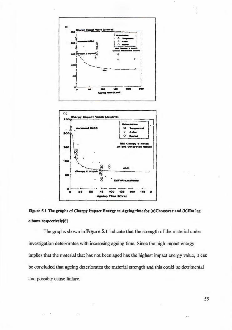
(a )
( b)
,oo~ I I I ·r
;--;;.:;..._~; , o-,I i ◊ ...... I ! I,~- 'I u:.=-:..-::..1
I
' ,::, 8 1 . I ... ______ .___ - i
-- - -'-'---1
l I I
o'------- ----- - ~---'
0 .. - - - -~-.......
2_ Oharpy lmpeot Value (JtCffl·a)
8 ANL
EdFn:,.._--.
o~~-- -------~- -~--o 21 50 70 100 120 1150 1711 2
~Tlfflelkllnl
Figure 5.1 The graphs ofCharpy Impact Energy vs Ageing time for (a)Crossover and (b)Hot leg
elbows respectively[6]
The graphs shown in Figure 5.1 indicate that the strength of the material under
investigation deteriorates with increasing ageing time. Since the high impact energy
implies that the material that has not been aged has the highest impact energy value, it can
be concluded that ageing deteriorates the material strength and this could be detrimental
and possibly cause failure.
59

5.2 CEMS MEASUREMENTS
In Figure 5.2 a typical Mossbauer spectrum obtained for natural iron (a.-Fe) that
was used for the calibration of the spectrometer is shown.
'ii' ....., C 0
1 t • C: a ~ • ► = CJ • °'
Na.tu.ral Iron 101.% ________ _;;,, ____ __,,,;;;;.;:;::;;;;a...:;aa;:;:;-
101.0
100.e
100.0
100.-4
100.2
100.0 ....... Fr--------...--., -10 0
Va;0city rmm/si] 10
Figure 5.2 Typical Mossbauer spectra for natural iron used for the calibration (maximum velocity 10
mm/s).
Pure a.-Fe, which is ofbcc symmetry and magnetic, gives a pattern consisting of
six peaks. The splitting between the first and the sixth peak is a measure of the magnetic
internal field. This magnetic field was found to be 33.77 Tesla for a 57Fe nucleus in pure
iron used as reference, and this is in accordance with the theory which gives the magnetic
filed for pure iron as approximately 33 Tesla [13]. The relative intensities of the six peaks
in a magnetically split Mossbauer spectrum depend on the angle between the direction of
the magnetic field and the direction of the gamma rays. Since a.-Fe can be easily
60

magnetised, and because of the saturation effects, the observed relative intensities from the
spectrum in Figure 5.2 are 3:4: 1: 1 :4: 3. For an absorption spectrum, the ratio 3:2: 1: 1 :2:3
holds if the gamma rays are perpendicular to the direction of the field. The doublet
appearing near zero velocity is the iron oxide (ex-FeOOH) due to oxidation of the top layer
of the iron.
The ex-Fe spectrum was used as reference standard for calibration purposes. The
spectrum for ex-Fe has six hyperfine components giving a linearity check. The energy of
the source transition was used as the arbitrary reference point when defming the isomer
shift, since the isomer shift observed depends on the type of the source matrix [12]. For
this investigation, the 57Co source, embedded in rhodium foil, was used. For the rhodium
foil, the isomer shift is +-0.113 mm/s. Adding this to the isomer shift for pure iron which is
-0.113 mm/s gives a value of 0.00mm/s. This is in agreement with the theoretical value for
the isomer shift of the commonly used 57Co source with respect to the iron metal at room
temperature, which is observed as 0.00 mm/s [12].
The calibration of the spectrometer was performed for velocities of 6, 8 and
1 0mm/s respectively and the calibration curves are shown in Figure 5.3. From the
calibration curves it is clear that the spectrometer performed according to specifications
and that the data obtained for the samples investigated would be acceptable.
61

Velocity vs Channel Number 250
. 200 0
z 150 Q) C:
ffi 100 .c: 0 50
0 -6 -4 -2 0
Velocity in mm/s 2
I--- 1 0mm/s --- 8mm/s -- 6mm/s
4
7 I I I I
6
Figure 5.3 Calibration curve for velocities of 6, 8 and 10 mm/s.
Figures 5.4(a) & (b) show typical Mossbauer spectra obtained for the duplex
stainless steel under investigation. All the spectra obtained for the different samples
consisted of a paramagnetic peak (singlet) and a magnetically split sextet. This singlet
arises from the austenite, which is a Cr-rich a-phase. A single line corresponds to an iron
impurity within a Cr-matrix and indicates a non-magnetic compound. The magnetically
split sextet resulted from the o-ferrite phase, which is a Fe-rich phase. The sextet
corresponds to iron with Cr as an impurity, which indicates that the iron atoms are in an
environment with at least one non-iron atom in the next nearest shell [6]. The separation
. between the lines is proportional to the magnetic field at the nucleus.
62

(a)
g 104
C 0 10.3 '!!I ~ C 102 0
,!:: .. .. 101 0 • ""
100
(b)
~hal:, ~ve-r CD - Bcxt..ct.
Rln.=b..ttlz:j
!\ I'
I\ I
0 v .. 1.,.,;fy [,...,m/c)
Ho~lcc MC
~ . .,,_. .... .. .
- 6 0 V•lac:rty [ml"Tl / c;: J
6
- S.,,xt,,et,
5
Figure 5.4 Typical CEMS spectra for (a) Crossover (b) Hot leg Elbows (Note: the small singlet is due
to an overflow of electrons and is part of the paramagnetic y-component).
The total contribution of the paramagnetic austenitic component was determined
to be in the range of 80 to 90%, represented by the singlet and the o-ferrite content was
found to lie between 10 to 20% which is represented by the sextet in the spectrum. The
error on the area computed for the o-ferrite component is relatively large due to the fact
that the sextet is obscured below the much bigger singlet of the austenite, which makes the
accurate determination of the area difficult.
Figures 5.5 (a), (b) and (c) show the typical Mossbauer spectra for stainless steel
63

alloy samples containing 64%Cr, 52%Cr and 30% Cr respectively. These samples were
used for reference purposes in order to prove that the magnetic field strength of the
samples investigated were correctly determined.
a)
F -, I i (b) '
,. ,. il r I
I
I I
i ... . ··· . · .. ,' _l
Figure 5.5 Typical CEMS spectra for stainless steel alloys with 64%Cr, 52% Cr and 30% Cr used
for reference respectively
64

The above spectra show that there is a shrinking of magnetic field strength towards
a single line with increasing Cr-content. The single peak is due to the fact that if Cr is
added to iron in diluted concentrations, a new structure appears in a Mossbauer spectrum
due to a reduction of the hyperfine field of the iron nuclei. Therefore the splitting of the
absorption lines will be slightly less, since the average hyperfine field of the whole pattern
decreases. Depending on the various possible iron-chromium configurations, a Cr-steel
will provide a pattern that is the superposition of all possible fields. With increasing
amount of Cr, the magnetic field shrinks as more Cr atoms surround the iron atoms [6].
Table 5.2 shows the hyperfine interaction parameters obtained for the natural
stainless steel samples that were used for reference purposes.
Sample
No
30% Cr
52%Cr
64%Cr
I NWU LIBRARYJ
Table 5.2 Mossbauer spectral analysis for Natural stainless steel
Isomer Shift (IS) Quadrupole Split Magnetic Field (H)
mm/s (QS) mm/s
Minimum Maximum Average
0.152 0.041 23.836 23.961 23.9
-0.09 0.022 15.361 18.961 17.2
-0.09 0.57 13.961 13.961 14.0
From the spectra, the total contribution of the austenite was determined to be
94%, 10% and 6% for the above alloys respectively. These values show that the stainless
steel with 64% Cr has iron atoms completely surrounded by Cr atoms, and this makes it to
be Cr-rich, and the magnetic field for this steel was found to be 14.0T.
65

A 30% Cr stainless steel is more Fe-rich, and this is indicated by the magnetic field
of 23.9 T which is higher than that of the 64% Cr. For the 52% Cr stainless steel, the
magnetic field was obtained as 17.2 T, which is an average of the high and low Cr
stainless steels.
According to Waanders et al (28] , there exists a linear relationship between the
magnetic field Hand Cr-concentration for various Fe-Cr-alloys and this was found to be
H = 33 .0 1 T - 29.61c
where c depicts the Cr-concentration (28], with errors of ±0.02 on both coefficients.
From the above equation, the magnetic field for the 30% Cr, 52% Cr and 64% Cr
used for reference purposes were found to be 23.13 T, 17.61 T and 14.06 T respectively.
These theoretical values fit in well with experimental values, which makes the calibration
to be satisfactory.
The nominal composition for the samples from ESKOM investigated is shown in
Table 5.3:
Table 5.3 Nominal composition of the duplex stainless steel under investigation
Element % Composition
Fe 67.4
Cr 20.0
Ni 10.5
Mo 2.1
From the above alloy composition, and if Cr, Ni and Mo are added as
approximation to give the concentration c, the value of the magnetic field strength H
should be about 27 T, for the type of steel under investigation. From the above formula,
66

the magnetic field for the samples was found to be about (23.35 ±0.02)T. This value is
similar to the magnetic field value obtained for the 30% Cr, which is about 23.9 T. The
ferrite under investigation contains about 10% Ni and 20% Cr as alloying elements which
cause the decrease in magnetic hyperfine field at the 57Fe nucleus.
In Table 5.4, the Mossbauer parameters for the sextet (6-ferrite), as obtained from
Mossbauer spectral analysis are shown.
67

Table 5.4 Mossbauer Parameters Spectral Analysis ( where no magnetic field is indicated, the
singlet component suppressed the sextet completely)
Sample Isomer Shift Quadrupole Split Magnetic Field (H)
Name (IS) mm/s (QS) mm/s
Minimum Maximum
CB 0.0077 -0.330 27.45 27.85
CD 0.1124 -0.048 24.00 24.00
CF -0.3969 0.155 24.91 25.91
CI 0.1433 -0.207 23.83 24.21
CM 0.2204 -0.119 22.81 25.01
CN 0.2652 -0.817
HB 0.0604 -0.332 29.13 33.13
HC 0.0518 -0.345 24.43 24.63
HD 0.2773 0.336
HE 0.0576 -0.375
HK 0.4630 -0.295
HM -0.2452 -0.851
HS -0.1038 0.073
The results in Table 5.4 show that values for the magnetic field strength determined
in the present investigation compare well with values found in literature. (IS: -0.02, QS:
varies, H: 27 T) [28].
68

5.3 SEM ANALYSIS
The microphotographs shovm in Figure 5.6 were obtained from the SEM
measurements. Figure 5.6 (a) shows the microphotograph for the sample with the low o
ferrite content and Figure 5.6 (b) shows the m.icrophotograph of the sample with a high o
ferritc content.
J P~•~ii '~ :;h\,~,-;\ '\ "''r>: ;j ta;~fiA__;;£~:.7·::.·,_:/J!~Li:<z~i-!,<~. ·::i~itJ
:-. -----·-! 200 um •·· ·--·-- ----- __ ____, :2 :_'; .:, 1.: :~;
Figure 5.6 Typical SEM microphotographs for samples with (a) low and (b) high 6-fcn ·ite content
respectively
On the photographs, the dark phase represents the a-ferrite and the austenite is
represented by the light phase. The amounts of the ferrite were found to be 10.08% and
22.24% for both Figures 5.6 (a) and (b) respectively.
69

The compositional variation of the samples, determined by means of the SEM fitted with an
EDAX are shown in Figure 5.7 (a) and (b) for the same samples which had a low and
high o-ferrite contents respectively.
W :20.0 Tlf\:0 .0 T1h~:U .O Tc :40
Lt,..c : M f t .Jvfl -11 " : l1 :01
EDU lAf Q.....,nt.<oc • hoft 1:.U.,,Hd!.u l E.,.,.... ,.tMeno, a li.l..d
" uL 1.\1 hit 0 . :1
I t ._:~ O. t l
6 1 . U O. H
\'),j,1 r H .o l 1"1 . 0!1
') . 30U I \Hl 0 , 11 • 1 : 'lO: • l ."D 1 . 001' I ') 0 " 0 , \\1 1
0 . 01,, o , 101 o . un :. 001 • ., =• o . :io:1 ::i , , 1 1 0 . ,, , 1 1 1011\ 1; II ) . 11\'I ') •PO O, U U
). II ,J.')O H 1 . ,1t 1 O . H :1 u .., o . ,n ·, .,, o . H11 1 cu : •
0 , ')011 ,) , '4 1 1 0 ,11 > ! ')J.JO 'I.D U I :a1 1 , lQ III
0.1 T~:.IVTW Ret : 141
FS: noo L-..c : 101
, .. l
EOA.l UJ O..,.,,ntifiuliofl (SIL.l~rcf le11I E\r-fl l NotTNo liucf
c: 1t :n.o , J llC: O, t)
l"o L l ,00 C r « 1' . 12 , .. ,, .. , 1'1111: !..O
Tot • l 100 . 00
,1.01 O.O U ) 1 . 114 1 O. llH t .OOO l O. t ) O. OOH t . 0'>11 O, H t l 1.00 11 O. Sl O. OlU O. H U O. I Ul I.DOU , .0 1 ll ll ( v 0 . • t 16 <,, U l i l.1101
1 1. \'l 1> . tJP O, tUl O, t 1 • : t.GOt) 1 , 41 1.1 . 0 11 t ,, . 1)S l 0. • lt~ l .OC,lnl
--------·---·· --------
Figure 5.7 Typical compositions for samples with (a) low and (b) high a-ferrite respectively.
·-
Tc::40
10:H:U
From the analysis of these samples, the amount of the different elements present in
the samples is in agreement with the chemical composition shown in Table 4.1.
70

The dark and the light phases in the samples were analyzed for Cr- and Ni-contents
in order to confirm whether they are the ferrite and the austenite phases respectively, and
the results are shown in Table 5.5.
Table 5.5 Cr- and Ni-contents of the dark and light phases.
PHASE ELEMENT WEIGHT PERCENTAGE(%)
Low o-content High o-content
Dark Cr 24.21 23.63
i 7.97 8.16
Light Cr 19.4 17.8
Ni 12.3 12.33
Table 5.5 shows the difference between the Cr- and Ni-contents between the two
phases present in the samples. In the dark phase, the Cr content is larger than in the light
phase, while the Ni content in the dark phase is smaller than in the light phase for both low
and high o-ferrite samples. According to Brown et al (27], the o-ferrite phase of the duplex
stainless steel contains more Cr than the austenite phase, while the content of Ni in the o
ferrite phase is smaller than that in the austenite phase (28]. From the results, the dark
phase is the o-ferrite and the austenite is represented by the light phase.
71

5.4 MICROSCOPIC IMAGE ANALYSIS
Figure 5.8 shows the microphotographs of Figure 5.6 (a) and (b) that were traced
onto the transparencies so that only the grains of the o-ferrite could appear and be counted
by the image analyzer.
, f" ' -
(a)
(b)
Figure 5.8 Samples with (a) low and (b) high o-ferrite content traced on transparencies.
72

Table 5.6 shows the results of the amount of o-ferrite as obtained from these
transparencies.
Table 5.6 &-ferrite content from photos traced onto transparencies
TYPE OF STEEL MEAN o-FERRITE (%)
Low ferrite content 10.1
High ferrite content 20.0
The amounts of the o-ferrite for both the samples are the same as those obtained by
Mossbauer spectroscopy and SEM analyses.
73

5.5 DISCUSSION
Charpy impact tests were used to follow the embrittlement of the steel. From Table
5.1, unaged samples have high impact energies and this energy decreases with increasing
ageing time. This implies that ageing deteriorates the material strength and this causes the
decomposition of the steel. The decomposition of the Cr-steel is mainly due to the diffusion
l N u I of iron and Cr atoms within the material [6]. LJBRARY. ' . -
According to Massoud [29], the embrittlement of duplex stainless steels during
ageing, at temperatures below 475°C, is basically due to micro structural evolution of the
ferritic phase. The main micro structural evolutions in the ferrite are the spinodal
decomposition of the ferritic Fe-Cr solid solution and sometimes the precipitation of the
inter-metallic compound. The spinodal decomposition leads to a fluctuation of the Cr
concentration corresponding to the formation of a' Cr-rich domains [29].
De Nys and Gielen [21] studied a 20 and 50 wt% Cr samples for two temperatures
of ageing, as shown in the spectra of Figure 3.11. From these authors, it was observed that
the sample with 20 wt % Cr induced a singlet near zero velocity at an ageing temperature
of 470°C, while no singlet was observed at ageing temperature of 540°C. For a 50 wt% Cr
sample, no singlet was observed at 470°C. At 540°C, the 20 wt% Cr sample lies outside
the spinodal region, while the 50 wt % Cr sample lie within the spinodal region at
temperature of 4 70°C, and this implies that at this temperature, this sample decomposes via
spinodal transition. The actual behavior of the 20 wt % Cr sample may have to do with
exact limits of solubility and impurities [30].
74

Many authors proposed that it is possible to differentiate between spinodal
decomposition and nucleation-and-growth by using Mossbauer spectroscopy. However,
according to Waanders et al [30] , the observation of a paramagnetic singlet or its absence
in the Mossbauer spectra of an Fe-Cr alloy, is an ambiguous rule as to whether the
embrittlement will occur via the spinodal decomposition or nucleation-and-growth
mechanism, as a singlet could indicate an advanced stage of spinodal decomposition when
the a ' -phase starts separating from the Cr-rich region formed during the early stage of
spinodal transition [30].
75

Table 5.7 shows the results of the mean a-ferrite content measured optically at the
ESKOM TRI center and by Mossbauer spectroscopy, done in the present research.
Table 5.7 Mean o-ferrite Values
SAMPLE NAME EQUIVALENT IMPACT /l. FERRITE /l. FERRITE
AGElNGTIME ENERGY (OPTICAL) (MOSSBAUER)
J/cm'
CB 75khr @ 291 l ° C 169.7 7.2 II
Cl ,,
156.5 7.7 10
156khr @ 291 I °C CN 144.7 5.8 8
,,
CM 122.3 6 .6 19
CF Start of Life 181.5 6 .0 10
No Spinodal
CD ,,
176.2 7.6 II
HC [email protected] ° C 82.9 8.6 21
HB ,,
77.6 9 .6 21
HS 15khr@325 ° C 130.2 7 .8 21
ITT . 110.5 9 .7 21
HE Start oflife 210.4 9.4 13
No Spinodal
HD ,,
97.3 10.1 12
HM [email protected] ° C 87.5 9.4 17
HK . 57.5 16.3 13
From the optical measurements, the a-ferrite content was found to be about 10%
for both Crossover and Hot Leg samples. However, from Mossbauer measurements, the o
ferrite content was found to lie between IO to 20%, represented by the sextet on the
Mossbauer spectrum.
The comparison of the mean a-ferrite content, as determined by optical and
76

Mossbauer measurements is in about half the cases not conclusive. This is so especially in
the case of Hot leg, due to the fact that the peaks of the sextet are obscured below the
much bigger singlet, which makes it difficult to determine the area covered by the sextet.
Therefore, the error on the a-ferrite component is relatively large. The results of both
optical and CEMS measurements show that there is no correlation in the amount of o
ferrite found in the samples.
The sample under investigation had about 20 wt % Cr and 10 wt % Ni as alloying
elements. This is a typical composition for duplex stainless steel containing both ferritic
(bee ex phase) and austenitic (FCC y phase) Fe compound. The Mossbauer spectra of all
the samples showed the appearance of the ex ' -Cr rich singlet near zero velocity, after
different ageing times and temperatures below 400°C. Mossbauer spectroscopy can detect
small Fe-rich concentration changes resulting in different phases developing during the
decomposition of the steel. According to Waanders et al [6], these changes can be
monitored by the measurement of the change in internal magnetic field that is proportional
to the Cr content of the Fe-rich phase. The average magnetic field for these samples was
found to be about 23 T. According to these authors, the average magnetic field increases
slowly with increasing ageing time, while the intensity of the paramagnetic singlet which is
formed due to the ex' -Cr rich phase, increases faster. However, for the samples under
investigation, this increase in the magnetic field with increasing ageing time is not evident.
This might be brought about by the fact that N~ which is one of the alloying elements, is an
austenizing agent [17, 18]. Addition of this element creates an austenitic micro structure,
and this reverses the effect produced by the addition of Cr in larger amounts, which creates
77

a ferritic micro structure.
The microphotographs from SEM analysis also indicate that the sample with low
and high 6-ferrite content had about I 0% and 20% 6-ferrite content respectively. The 6-
ferrite phase is represented by the dark phase on the microphotographs whereas the
austenite is represented by the light phase.
The results of SEM fitted with an EDAX reveal the compositional variations for
both samples with high and low 6-ferrite content. The 6-ferrite phase of both samples
contains about 24 wt% Cr and 8 wt% Ni, while the austenite phase of both the samples
contains about 19 wt% Cr and 12 wt% Ni. According to Brown et al [27] , the 6-ferrite
phase of the duplex stainless steel contains more Cr than the austenite phase, while the
content of Ni in the 6-ferrite phase is smaller than that in the austenite phase.
5.6 CONCLUSION
There is no clear correlation between the 6-ferrite content and Charpy impact
strength values. From the impact strength measurements, the impact energy decreased with
increasing ageing time. If the impact energy decreases, the hardness of the stainless steel
will be reduced and this would lead to the degradation of the stainless steel. The reduction
in the hardness of the steel is brought about by the fact that during ageing of the stainless
steel, there is a micro structural evolution of the ferrite phase to a hard and brittle Cr-rich
phase. However, the increase in 6-ferrite with increasing ageing time is not evident. Thus,
some other mechanisms might be responsible for the decrease in impact energy.
From Mossbauer measurements, the average magnetic field for the samples
78

investigated was found to be about 23 T. Theo-ferrite component for both the Hot leg
and the Crossover leg samples were found to be about 10% to 20%, whereas the austenite
component was found to be about 80% to 90%. However, no correlation was found
between the amount of the o-ferrite in the samples and their ageing times, as determined by
CEMS measurements.
The SEM results reveal the two phases present in the samples under investigation.
One of these phases is the ferrite phase represented by the dark area on the
microphotographs of Figure 5.8, and the content was found to be 10% and 20% for the
samples investigated. The other phase that was observed is the austenite represented by the
light area on the microphotographs. This phase was found to be about 80% and 90% for
the samples investigated. For all the samples investigated, the o-ferrite contains about 24
wt % Cr and 8 wt % Ni, while the austenite phase for the samples contained about 19 wt %
Cr and 12 wt% Ni. This is in agreement with the results by Brown et al [27] , that the o
ferrite phase of the duplex stainless steel contains more Cr than the austenitic phase, while
the Ni content in the o-ferrite phase is smaller than that in the austenite phase.
The samples used in this investigation had about 20%wt Cr and these samples were
aged below 400°C. At this ageing temperature, the samples showed a large singlet near
zero velocity. These samples are thought to decompose via spinodal decomposition.
5.7 RECOMMENDATIONS
The current research shows that the impact energy decreased with increasing ageing
time. This decrease in impact energy indicates the degradation of the stainless steel.
79

However, the increase in a-ferrite with increasing ageing time is not evident. Thus, some
other mechanisms might be responsible for the decrease in impact energy. Therefore, the
measurement of other mechanical properties is suggested.
The Mossbauer spectra of all the samples investigated showed the appearance of
the Cr rich singlet near zero velocity. Mossbauer spectroscopy can detect small Fe-rich
concentration changes resulting in different phases developing during the decomposition of
the steel. These changes can be monitored by the measurement of the change in internal
magnetic field that is proportional to the Cr content of the Fe-rich phase. The average
magnetic field for these samples was found to be about 23 T. However, there is currently
no sufficient information on the mechanisms of the embrittlement by either spinodal
decomposition or by nucleation-and-growth. The author therefore suggest the use of
Mossbauer Spectroscopy for samples aged at various temperatures in order to follow the
steps in the spinodal transformation. This can be done by choosing a temperature at which
the Cr rich region will appear paramagnetic [30]. Since Mossbauer spectroscopy can assess
how far the transformation has advanced, this technique can also be employed to determine
the activation energy of embrittlement in the case of nucleation-and-growth. The simulation
of the plot of spinodal decomposition for an alloy with 20 wt % Cr and 10 wt % Ni is also
suggested, and the results can then be compared with the experimental results found by
Mossbauer spectroscopy. l NWU LIBRARYJ
In order to describe what happens at the atomic level when the Cr steel is aged, the
micro structural changes in the stainless steel alloy can be investigated by using atomic
probe techniques such as ion field microscopy(IFM).
80

The samples under investigation had about IO % Ni as the main alloying element.
However, there are some other impurities like Si, Mn, Mo and Cu. It is also recommended
that the effect of these impurities on the type and degree of transformation be investigated.
The effect of Ni as a function of these impurities needs also to be investigated.
81

BIBLIOGRAPHY
1. Ishikawa Y, Yoshimura T, Moriai A and Kuwano H. Materials Transactions, TIM,
36(1995), 16-22.
2. Kuwano H, Ishikawa Y, Yoshimura T and Hamaguchi Y. Nuclear Instruments and
Methods in Physics Research, B76 (1993), 290-291.
3. Brown J E and GD W Smith. Surface Science, 246(1991), 285-291.
4. Morimoto K, Hirihigashi A and Nasu S. Nuclear Instruments and Methods in
Physics Research, B76 (1993), 295-296.
5. Jansson C .Degradation of Cast Stainless Steel Elbows after 15 Years of
Operation.
6. Waanders F B, Pollak Hand Karfunkel U. Life Time Assessment of Steel Vessels.
7. Mossbauer R L. Science, 137,731(1962)
8. Cohen R L. Applications of Mossbauer Spectroscopy Volume I, 1976, Academic
Press Inc.
9. Parish RV. NMR, NQR, EPR and Mossbauer Spectroscopy in Inorganic
Chemistry, 1990, Ellis Horwood Ltd.
10. Long G J and Stevens JG. Industrial Applications of the Mossbauer Effect, 1986
Plenum Press.
11. Srivastava C M and Srinivasan C. Science of Engineering Materials, 1987, Wiley
Eastern Limited.
12. Wertheim GK. Mossbauer Effect: Principles & Applications, 1964, Academic
Press Inc.
82

13. Straughan BP and Walker S. Spectroscopy Volume I, 1976, Chapman and Hall
Ltd.
14. Schneider G. Untersuchung von Nickelhydrid unter hohem Druck mil Hilfe der
Mossbauerspektroskopie an 57Fe, Juli 1989.
15. Krane K S. Introductory Nuclear Physics, 1988, John Wiley & Sons Inc.
16. Greenwood N N . The Mossbauer Spectra of Chemical Compounds, Chemistry in
Britain, 1967, p56-72.
17. Llewelyn D T. Steels : Metallurgy and Applications, Second Edition, 1992,
Butterworth-Heinemann Ltd:
18. Potgieter J H. British Corrosion Journal, 1992, 27(5), 219-223.
19. Smallman RE. Modern Physical Metallurgy, Fourth Edition, 1985, Butterworth
Heinemann Ltd.
20. Smith W F. Principles of Materials Science And Engineering, Fourth Edition,1996,
McGraw-Hill Inc.
21. De Nys T and Gielen MP. Metallurgical Transactions, May 1971, Volume 2,
pl 423.
22. Chandra Band Swartz L H. Mossbauer Effect study of the 475°C decomposition of
Fe-Cr, Metal.Trans. 2 (1971), 511.
23. Vander Voort G F. Metallography Principles & Practice, McGraw-Hill Book
Company.
24. Thornton PA & Colangelo VJ. 1985, Fundamentals of Engineering
Materials, prentice-Hall, Inc, p23 7-23 9.
83

25. Moodley MK. The Construction of a CEMS detector and its Application to the
Study of Fe-Silicides, Unpublished Msc Thesis, UDW.
26. Phillips VA. Modern Metallographic Techniques and their Applications,
1971,p425.
27. Brown J E, Hetherington MG, Smith GD, Pumphrey PH. Fatigue, Degradation
and Fracture, A.S.M.E, New York, 1990, Volume 195 pl 75-177.
28. Waanders F B, Vorster SW and Pollak H .. Mossbauer Parameters for High
Chromium Stainless Steels, Hyperfine Interactions C3(1998) 281-284.
29. Massoud JP, Auger P, Danoix F, Rezakhanlou Rand Van Duysen JC. Evaluation
of Thermal ageing of Duplex Stainless steel, Ed RE Gold and EP Simonen, The
Minerals, Metals & Materials Society (1993) 399-405.
30. Waanders F B, Pollak Hand Karfunkel U. Fe-Cr System by Mossbauer
Spectroscopy. Unpublished Report.
31. Geldenhuys A: Content of Delta ferrite in Austenitic Stainless Steel, Unpublished
Fourth Year Project, Potchefstroom University.
84

APPENDIX A - CEMS SPECTRA
In this Appendix, Mossbauer spectra for natural iron
used for the calibration of the spectrometer at velocities of
6, 8 and 1 Omm/s are presented. The spectra for the stainless
steel samples used for reference purposes as well as for all
the samples under investigation are also presented.
85

APPENDIX Al Spectra obtained for natural iron used for calibration
purposes.
86

Al .1 Natural iron: 6mm/s velocity
I , :u ~ ,.; - - ---·--- - : '.J
-- ----• - -- - -----' i:.
\'_\.I '
·:, ,,:: ,:;_ =.;.: -· .. - . - -··- --- -- - - -- --- ·· - · - . -· .
Chw '"" l riu111lx ,r · 5 1 2 Fo ldingvoiril 256.S C (!OOl . Ff f cc L 1 S
Jun l!l 1998 l 2:S7:,\l
Sl'H0O C::n l ibrnti o n -· 6u 1:c - foil rr
·n,cor·y '.l Numb~ : r· qf J>1 1 r ·• u1H! l <! r·:.; 10 Numtx!r· of l le r-; 1 l i n n =:; 7 Chi' 2 .6286
Nct.n1e lni l iul Finul 1:: rr-c,r Chec k
base l i n r, 7.'3 4!1 6307 7 . 4631 I .000 1 . 000 To tal Ar- eo - 0 . 7500 -- 1 . 2584 0 .0109 1.987 l. 988 Mng f" i c,ld 33.0000 '.l3. 4804 0. Ol Ol 0 . 988 0 .958 Quad ~fr.v,: 0 .0030 0 .02 12 0 0024 0.976 0.980 Shif l Mt..11,; -0. l 100 - 0. l 03'.) (l . 001'.l 1 . 05 l 1 . 058 Width OJl 0.3t.OO 0 .28::>7 C .004U 1.342 1. 282 W id ti , Mid 0 .3000 C.2787 0 . 00 46 1.847 l. 75 l Width l:nn 0 .2500 0.3298 0. 0101 1 . 162 0 .992 A r t?a ( AJ l 0 .5000 0. 3607 0 . 0036 l .923 l . 918 Arcu Mi.d 0 .3500 0. 4 583 0 .004t. 2.810 2.012
87

Al.2 Natural 1ron: 8mm/s velocity
Knllibrnsic, GEMS OP!:;lcsll. int.: 15/10/9fl
Channc l numbc r Fold i ng-po int: Geom. F.ffc,ct
5 12 25fi.5
3437
. . ... :,..• . .-·
R""u 1 ts o f Fil 0c t I 5 l !J!l!l 13 : 09: 02
Sf'fl00 - Cnl ibrntion - Gu Fc - foi l u
Theo r.v : ::i N1Jmbe•· o f Pr,rfl.llletcrs Chi'
10 Number of rtc, rnti.on,:;
Nrunc
bllsel inc Total Arca Mni;: Fic,lci Quad M, J.J; Shi ft. 1,l.,g Width O..,t Wicilh Mid Wi.dth Inn Arca Oul
Ar0.n. Mid
l. 1663
fniti11 !
10061.41) -0 . 0500 3:1.0000
0 . 0030 -0 . l 100 0 . 3400 0 . 3000 0 . 2500 0. 5000 0 .:1:iOO
Finnl f~r-r o r
1.005835 67.4130 -0. 0 430 0.0005 33. ~5lfl 0 . 0194 -.o . 0030 0 . 0046 :.Q-JJ .Z0 0 . 0025
0 . 3690 0.0094 0.2992 0. 0079 0 . 4538 0.0229 0 . '.194] 0.0065 0 . 4052 0 . 0076
I_ NWU IJJBRAnvl 6 -
Check
1 . 000 1 .000 1 .526 1 . 529 0.995 0.%1 0.955 0 . 99l1 1 . 152 l . 087 1.410 1. 32'.l 2.012 l . fl72 1.173 0.875 2.0~ll 2.0H5 3 . 142 3. I 2S
88

Al .3 Natural iron: 1 Omm/s velocity
yk i ni:;- op l . 0n ■n/ s 18/6 /98
Chunnc l r 1u111 lx, r· 1:0 Id i n g-poin l Ccnm . 1-: f f <:Ct
512 256.5
- 63
GC
ll,, ,;ul le, of Fi L Ju11 JI\ J'.l9H 12:1\2:16
srv,:ioo Cn l ibralion ·- Gu Fe - foi l tt
Theory 3 Nu111lx? r· of l \:, r-ome t c r ! ·; 10 Number- o f J Le ri, t ions : G
Chi' 7.6952
N c: Ull<! l ni Li ul Fir1nl Er-r-or Che c k
bo:;e l i.n c 22598 22598 24.8583 I . 000 l . 000 Toto! Arco - 1 . 2204 - 1 . 220 1\ 0. 0 1 13 1 . 528 l. 53 1 Mag F ield 33.2 403 33 . 2403 0.01 33 0.994 0.930 ~ad J.<a g 0.00 19 0. 00 19 0 . 0032 0.955 0.981 Shi ft Mn.g - 0. 1091\ -0 . 10!) 4 0 . 0017 t . 049 1 . 042 Wid th Cut 0.3222 0 . 3222 0 . 0063 1.297 1.363 Wid th Mid 0.2850 0 . 2850 0 . 0055 l . 639 1.386 Wi dth I nn 0.3292 0 .3292 0 . 01 2 1 I.. 132 0.964 A, ·et::a Cut 0. J9 '.){l (). :J9~}[1 0.00 .-: 2 1 .827 1 . 7~3
An.:a Mid 0. 4238 0 . I\ 238 0.0052 2.GG5 2.73 1
89

APPENDIXA2 Spectra for stainless steel used for reference purposes.
90

A2.1 Stainless steel:
·•-::-•
30%, Cr
,. I .. ,
___ _..~ ..
U~7HI~• •,l,f:IIIJ
:I, 0:111:ii~I) :z..O~Oc»o
::l).U.SH 11,.1.dH •O,HIOD 'I' ~ .1-t-.,11 0 •• 0101 " ,.,.,. r, . ao,:~ P' i:>.uac.1 11.tOIGC P 0.fJ'J,~1
C:.Ct~H ~ . fl:'IICIIIIO a.~~on 1.0::io::.o 0.0::,000 ,,aooH 0 .0::1000 D,DCIIICICI o .uc:IJ(:i;, (1,0(100(l' ll(IGOe D OIICIIC ~.OOIIQC ~.,uuuc
... _.._ ... ~, 14
C: . DII,~ r.. t,~:, r. • ')Cl "I c.~;t e.,o:, i:.ao C.QU ; ,GIIQ I:, GUO t .oo~ ,.,.,c: 0 lll'JO O.IIOQ 0.000
I, IILILI o.uoo ft UIR .,HO O.OOCI ,.::1:11, I, :,:io •• ~::ii, L :t~l:t o.~,o ,.,,c, ~ - ~ i=.~~ :. ::101)
..
91

A2.2 Stainless steel: 52%Cr
fitresults of data 52% Cr
foldingpoint geometryeffect theory dat:e t:1.ags titspac:tra c:hi2 c:hi2-test corr - te6t fitcyclee maxiter parasig chi2Big fitpar.ameter Bas .. J.ine '1.'otal Are11 Sexteta Doublets Hag Pi,.1.d l. Quad Mag l. Shi.ft M•g l. Width Out l. 3 : 2:l. Corr WNat Mag 1 Quad Split Is:o Shift l Width l. Area 1
l.
254.5 0.032 ~
C:\PCMOS\NSext . exe Sun Jan 2 8 22:41: 26. 2001 ---c- -
l. l..3293 0 . 0000 \-0 . 0000 \-
13 25
l. l.
14 62071.831
- 0.00810 l..00000 l. . 00000
l.8 , 96120 0.47000
-0 . 09100 0 . 30000 1. ·08000 0 . 25.900 0.00000 0 . 24000 0 . 46600 0.1.5700
62069G77 - 0.00565 l.00000 l..00000
l.5 . 36 "144 0 . 02158
-0 . 09100 1. l.8226 3 . 10238 1 . 93491 0 . 00000
-0. 01154 0 . 46600 0 . 094 34
l'
F
p
..
0.00000 0 . 000 0.000 0.00000 0.000 0 . 000 0 . 00000 0 . 000 0 . 000 0 . 00000 0.000 0.000 0 . 00000 0 . 000 0.000 0.00000 0.000 0 . 000 0.00000 0.000 0 . 000 0.00000 0.000 0 . 000 0.00000 0 . 000 0.000 0.00000 0.000 0 . 000 0.00000 0 . 000 0 . 000 0 . 00000 0.000 0 . 000 0 . 00000 0.000 0 . 000 0 . 00000 0.000 0.000
92

A2.3 Stainless steel: 64%Cr
- ~11:ar I!••• ur-
254.5
fitresults of data monster 2 G41 Cr foldingpoi.nt geometryet:fect theory
0,025 \C:\PO!OS\N6ext . exe Sun Jan ~8 2~,S0 : 4 S date 2001
fl.•gs titGpectra chi 2 chi2-test corr-test fitcycles maxiter paL·asig chi2s i g .fit.parameter Baseline Total. Area Sextets Doublets Mag Field l. Q,,.ad Mag l. Shi t:1.. M11.g l. Width out l. 3 : 2 ,l corr WNat Mag l. Quaa Spl.it ISO Shil'.t l. Width l. Area l.
1
---c- -1. o .ss,J 0.0000 't 0.0000 \-
10 25
l. l
l.4 2!>020889
-0 . 00810 l..00000 1.00000
13. 961.20 0 . 47000
-0 . 09100 0 . 30000 1.08000 0 . 2§900 0 . 00000 0 . 24000 0 . 4G600 0 . 85700
;!l)Ol.6334 0 . 00099 l. ,0 0000 1.00000
1.3. 96120 o . ~1so1
-0 . 09 1.CO 0 . 011944 l..l.88J2 0 . 531 '/S 0.00000
- 0 .235 88 0.351.64 o . !B541
F
F
Ii'
F
I Par....,t.ars : .1.•
0 , 00000 0 . 000 0.000 0.00000 0 . 000 0.000 0.00000 0 .000 0.000 0 . 00000 0 . 000 0 .000 0.00000 l..000 J..000 0.00000 0.000 0 . 000 0 . 00000 l. . 000 1 . 00 0 0.00000 0 . 000 0 .000 0.00000 1 . 000 l. . 000 0 . 00000 0.000 0.000 0.00000 .l.. 000 l. . 000 0 . 00000 0 . 000 0 . 000 0.00000 0 . 000 0.000 0 , 00000 0.000 0.000
93

APPENDIXA3 Spectra for crossover samples under investigation
94

Rinchale Ci.om n:r CB - Bcxtet.
~ 1......1 106
C 0
·gi "t 10'4-... C 0
..= 102
1 00 .. _ • - ... --6 0
VAlc:u:~lty [mm/a:] 6
Parame t e rs f or NSext : N magneti c s extets and M quadrupole doubl e t s • fitresult s of data : s ample c rossover leg cb foldingpoint geometryeffe c t theo ry date fla1r s f itsp e ctra chi2 ch i2 - test corr - test fit c ycla s max i ter parasi1r ch i2 sig fitparameter Bas e line Total Area Sextets Doublets Mag F i eld l Quad Mag 1 Shift Mag l Width Out 1 3:2 : 1 Corr WNtit Ma g l Quad , :pl it l I s a s hift 1 Width 1 Arett Quad split. l :;o s h i f t Wid th Ar e n
1 2 2 2 2
255 . 0 0.202 %
C: \PCMOS\NSext . exe Fr i Oct 23 14 : 54 : 58 - --CE -
1998
1 7 . 2260 0.0000" 0 . 0000 X 8
2 5 l 1
18 3 157981 - 0 . 03750
1 . 00000 2. 00000
24 . 21330 - 0. 03530 - 0 . 11590
0 . 11400 1. 00000 0.25000 0 . 00000
-- 0 . 209 30 0. 3Gl00 0 . 58 740 0 .00000 0 . 187 :IO 1 . 3 9 6 40 0 . 10720
3165043 - 0 . 0408 0
1 . 00000 F 2 . 00000 F
21 . 94105 - 0 . 11534
0 . 10 2 0 7 0 . 82860 1 . 0000 0 r 0 .25 000 F 0 . 000 00 l7
-- 0 . 21 3 :J 9 0 . 3767 3 0 . 1,, 776 1 0 . 0000 0 r, 0.187 3 0 F 2 . 9145 9 0 . 206 'l4
. \.
I NWU-1LIBRARY_
191 . 07811 - 0 . 882 3 . 180 0 . 00053 - 1 . 121 3 . 5!)9 0 . 00000 1 . 000 1 . 0 00 0 . 00000 1 . 000 1 . 000 0 .2 7342 0 . 810 0 . 542 0.0 5 922 4 . 812 - 1.870 0 . 03122 ·· l. 6 5 7 4 . 954 0 . 1 3 45 8 4 .536 - 0.6 3 7 0 . 0 0 000 1 . 0 00 1.000 0 . 00000 1 . 000 1 . 00 0 0 . 0 0000 1 .000 1 . 0 00 0 . 00114 1 . 444 0 . 6 25 0 . 00 38 5 1 . 6 59 1 .3 32 0 . 01103 0 . 11 7 2 .3 32 0 . 00000 1 . 000 1 . 000 0 . 00000 1 . 00 0 l . 00 0 0 . lfi 544 ·J . 2 09 3 . 478 0. 01 1 04 -- 0 . 56 0 4 . 222
95

~ 10-4-
1 t .. C 0 ~ 102
• ► ;: 0 • a,:
100
Rinehals ~r CD
-6 0 V•lcu:lty [mm/,.]
Sextet,
6
Parameters for NSext : N magnet ic fitresults of data :
sex tet s ttnd M quadrupo le doublets
254.5 sample CD Crossover foldingpoint geometryeffect theory
0.203 % C:\PCMOS\NSext.exe Mon Oct 26 10:33 : 13 ---CE-
date flags fitspectra ohi2 chi2-test corr-test fitcycles maxiter parasig chi2sig fitparameter Baseline Total Area Sextets Doublets Mllg Field 1 Quad Mag 1 Shift Mag l Width Out 1 3 :2:l Corr WNot Mag 1 Quad split 1 Iso shifl 1 Width 1 Area Quad split Iso shift Width Arett
1 2 2 2 2
1 5.8779 0 . 0000 % 0 . 0000"
22 25
1 1
18 3432453 - 0 . 03160
1 . 00000 2.00000
24.21330 -0.03530 -0 . 11590
1 . 11400 1.00000 0 . 25000 0.00000
- 0.21610 0 . 37530 0. 60160 0.00000 0.22030 1.17550 0.20920
1998
3426630 - 0 . 03228
1 . 00000 F 2 . 00000 F
19 . 95558 - 0 . 04899
0 . 11238 0 . 74576 1 . 00000 .F 0 . 25000 F 0 . 00000 F
- 0 . 19728 0 . 42039 0.75848 0 . 00000 F 0 .5 6873 1. 05669 0.13084
186.57775 3.545 -- 1. 265 0 . 00046 4.187 -1. 695 0 . 00000 1.000 1 . 000 0.00000 1.000 1 . 000 0 . 29769 0 . 731 0 . 332 0 . 06869 3.834 0 . 272 0 .03 644 0.258 4.352 0.13613 0 .7 54 2.704 0 . 00000 1.000 1 . 000 0 . 00000 1.000 1 . 000 0 . 00000 1 . 000 1.000 0.00131 1.823 -0 . 010 0 . 00449 3. 310 0 . 328 0 . 01239 5 . 208 -2. 449 0 . 00000 1.000 1. 000 0 . 00863 3 . 144 0 . 079 0 . 07135 - 1 . 496 3 . 939 0 . 00666 --0 . 893 2.99 0
96

ftinahnh, Cxumu¥Ur CE1 ...,_. BoxtA:,t.
C 0
11 '{; tll C a ~ • ,. :;: 0 • a,:
101.0
100.5
-6 0 VAloclty [mm/•]
Parameters for NSext : N magnet i c s extets and M quadrupole doublets fitresults of data Ringhals Crossover Sample CE1 foldingpoint 267.0 geometryeffect 0.187 % theory C:\PCMOS\NSext.exe date Mon Oct 26 10 : 01 : 54 1998 flags - - - CE-fitspeotra 1 chi2 1.0054 chi2-test 46.4252 " corr - test 20.8672 " fitcycle s 9 maxiter 25 parasig 1 chi2sig 1 fitparameter 18 Baseline 6175905 6174665 Total Area - 0 . 03750 -0 . 00794 Sextets 1.00000 1 . 00000 Doublets 2 . 00000 2 . 00000 Mag Field 1 21 . 85120 20 . 77906 Quad Mag 1 - 0 . 33530 - 0.47674 Shift Mag 1 -0.11590 -0 . 09505 Width Out 1 1. 21400 0.37768 3 : 2 : 1 Corr 1.00000 1.00000 WNat Mag 1 0 . 25000 0.25000 Quad Split 1 0.00000 0.00000 Iso Shift 1 ·-0. 22696 -0.21286 Width 1 0.36600 0.47137 Area 1 0 . 12452 0.79990 Quad Split 2 0 . 00000 0 , 00000 Iso Shift 2 0.53400 0 . 63830 Width 2 1 . 02100 0 . 96097 Area 2 0 . 19400 0 . 10657
222.60390 0.00027
F 0.00000 F 0.00000
0.39824 0 . 10489 0 . 05336 0.18634
F 0 . 00000 F 0 . 00000 F 0.00000
0.00435 0.01422 0 . 03039
F 0 . 00000 0.03173 0 . 22008 0 . 01817
1.013 0.957 1 . 000 1.000 0 . 635 1 , 361 2.140 1.309 1.000 1.000 1.000 0 . 869 1.329 0.995 1.000 0.997 0.978 0.982
0 . 917 0. 911 1.000 1.000 1 . 304 1 . 670 0 . 821 0. 644 1.000 1.000 1.000 0.994 0.992 0 . 830 1.000 1.340 0.815 0 . 887
97

Rin,ch.a.h, C:umu n::::r CF - Sextet.
...... N ....., C 0
1 l; .. C C ~ • > ~ 0 • °'
101.0
100.8
100.e
100.4
100.2
100.0
-6
•
0
V11h:u:lty [mm/ a] 6
Parameters for NSext : N mar;netic sextets and M quadrupole doublets fitresul~s of data Ringhals Crossover Sample cf foldingpoint .. 255 . 0 geometryeffect 0 . 185 " theory C:\PCMOS\NSext.exe date Mon Oct 26 10:55 : 54 1998 flags ---CE-fitspectra 1 chi2 0.8984 chi2 - test 87.1250 " corr - test 66.1670 " fitoycles 12 maxiter 25 parasig 1 chi2sig 1 fitparameter 18 Baseline 6504502 6504519 247 . 95207 0 . 763 Total Area -0 . 03750 - 0.00616 0.00031 0 . 633 Sextets 1 . 00000 1 . 00000 F 0 . 00000 1.000 Doublets 2.00000 2.00000 F 0 . 00000 1.000 Mag Field 1 24.21330 24 . 21330 F 0 . 00000 1.000 Quad Mag 1 -0.03530 0 . 15558 0.15734 0.421 Shift Mag 1 - 0.11590 -0.39697 0.07928 0.386 Width Out 1 0 .11400 0.44060 0.31349 3.401 3 : 2:1 Corr 1.00000 1.00000 F 0 . 00000 1.000 YNat Mar; 1 0.25000 0.25000 F 0.00000 1.000 Quad split 1 0.00000 0.00000 F 0 . 00000 1.000 Iso shift 1 - 0.30030 -0.21555 0.00508 0 . 897 Width 1 0.36100 0 . 46756 0 . 01593 1 . J 08 Area 1 0 . 58740 0.84500 0. 04424 0 . 695 Quad split 2 0.00000 0.00000 F 0 . 00000 1.000 Iso shift 2 0 . 18730 0 . 57126 0 . 03169 1 . 004 Width 2 1 . 37220 0 . 62411 0 . 21917 1 . 427 Area 2 0.20970 0 . 06457 0 . 01678 1 . 122
1 . 278 1. 478 1.000 1 . 000 1 . 000 0.918 0 . 942 0.420 1 . 000 1 . 000 1. 000 0 . 933 1 . 143 1 . 416 1 . 000 1.026 0.676 0.852
~·
98

fitresults
• ► :;:: 0 • a:
of
106
104
102
100
da ta
Rin,Kbals CroS90~r CI - Sextet
-6 0 6
V•IQc::lty [mm/i::]
: sample ci cros sover l eg fol d ingpoint 255. 0 geo111etryeffect 0 . 191 " theory C : \PCMOS\NSext.exe date Mon Oct 26 11 : 18:32 1998 fl a gs - - - CE -fitspect ra 1 chi2 2 . 9469 chi2 - test 0 . 0000 " corr-test 0 . 0000 " fitcy c le s 9 111axiter 25 parasig 1 c hi2siG" 1 fit parame ter 18 Baseline 1 903544 1900805 153 . 99841 -1.445 Tot11l Area - 0.03360 - 0.03182 0.00072 -1.934 Sextets 1.00000 1.00000 F 0.00000 1.000 Doublets 2 . 00000 2.00000 F 0 . 00000 1.000 Mag Field 1 24 . 21330 24 . 21330 F 0 . 00000 1 . 000 Quad Wag 1 -0.03530 - 0 . 20712 0 . 10842 2. 161 Shift Mag 1 - 0 . 11590 0 . 14331 0 . 05617 2 . 687 Width Ou t 1 1.11400 0.76490 0 . 23286 3 . 001 3:2:1 Corr 1.00000 1 . 00000 F 0 . 00000 1,000 WNat Mac 1 0.25000 0.25000 F 0 . 00000 1.000
. Quad split 1 0 . 00000 0 . 00000 F 0 . 00000 1 . 000 Iso Shift 1 - 0 . 20470 - 0 . 20395 0.00169 1. 338 Width 1 0.37380 0 .41029 0 . 00572 2 . 074 Area 1 0.62010 0. 7,7317 0 . 01898 -1.539 Quad split 2 0 . 00000 0 . 00000 F 0.00000 1 . 000 Iso Shift 2 0.27310 0 . 54573 0.01078 0.768 Wi dth 2 0 . 86890 1 . 04959 0 . 09044 0.936 Ar ea 2 0 . 20800 0 . 13085 0 . 00882 - 0 . 311
3 . 505 4 . 027 1 . 000 1.000 1.000 2.569 2.497
- 0 . 846 1 . 000 1.000 1.000 0.517 1.717 3. 911 1.000 1.922 1. 396 2.241
99

Rizichah:,' 01.~•ur CM """ ~
C 0
1 t .. C D ~ • ,. = g • c,i:
100.8
100,C
100.4
100.2
100.0
-6 0
ValAc:=lty [mm/ •1
Sample CMl 256 . 0
f tresults of data R nghals Crossover f ldingpoint geo111etryeffect theory
0 . 183" C:\PCMOS\NSext . exe Wed Oct 28 12:17 : 17 ---CE-
date flo~s fitspectra
1998
chi2 chi2 - test corr-test fitcyoles maxiter parasig chi2sic fitporo111eter Ba1.eline Total Area Sextets Doublets Nae Field 1 Quad Mag 1 Shift llag 1 Width Out 1 3 : 2 : 1 Corr WNat Mac 1 Quad split 1 Iso Shift 1 Width l Area 1 Quad split 2 Iso Shift 2 Width 2 Area 2
1 0 . 8318
97.3952" 98 . 9610"
5 25
1 1
18 6221510 -0.05360
1.00000 2.00000
24.21330 -0 . 07506
0.21669 1. 22400 1 . 00000 0.26000 0 . 00000
-0 . 20116 0 . 45524 0. 1j043 0.00000 0.61695 0 . 71267 0.0{)262 ..
6221886 - 0 . 00484
1 . 00000 F 2.00000 F
24.21330 F -0 . 11945
0 . 22037 0.94266 1.00000 F 0.25000 F 0 . 00000 F
-0 . 20811 0.43843 0 . 74888 0 . 00000 F 0.52743 0 . 46622 0.06019
293 . 88868 0 . 00043 0 . 00000 0.00000 0.00000 0 . 25967 0 . 13717 0 . 56535 0 . 00000 0 . 00000 0 . 00000 0 . 00692 0.02186 0.07153 0 . 00000 0 . 02578 0 . 18608 0 . 01846
1.153 1.121 1 . 000 1 . 000 1 . 000 2.496 1 . 723 0.220 1 . 000 1 . 000 1 . 000 1. 282 1 . 222 1 . 218 1.000 0 . 928 1.213 1.010
0 . 616 0 . 586 1 . 000 1 . 000 1 . 000 1.497 2.599 0.693 1.000 1 . 000 1 . 000 0 . 883 1.660 0 . 404 1.000 1 . 263 0 . 629 0 . 725
100

,..... N! ....... C 0
11 i; -C C
i!:: • ,. :;:: C • 0.:
108
104
102
,oo
Crossover Leg 254.5
fitresults of data sampie co Ringhals foldingpoint geometryeffect theory
0 . 192 % C ( \PCNOS\NSext . exe Tue Oct 27 09 : 33:10 - --CE-
date flairs fitspectra chi2
1998
chi2 - test corr-test fitcycles maxiter parasig chi2sig fitparameter Baseline Total Area Sextets Doublets Mag Field 1 Quad Mag 1 Shift lr!air l Width Out l 3: 2: 1 Cor-r WNat Mag 1 Quad split 1 · Iso Shift 1 Width 1 Area 1 Quad split 2 Iso Shift 2 Width 2 Area 2
1 4.3283 0 . 0000" 0 . 0000 % 9
25 l 1
18 1580680 - 0 . 05360
1 . 00000 2 . 00000
24 . 21330 -0 . 03530 -0. 11590
0 . 91400 1.00000 0 . 25000 0 . 00000
-0. 35470 0 . 58440 0 . 63140 0.00000 0 . 42290 0.77550 0.21230
1581741 - 0.03542
1 . 00000 2.00000
24 . 21330 -0.81749
0 . 26524 ] . 33519 1 . 00000 0.25000 0 . 00000
-0.20212 0 . 41761 0 . 79,573 0 . 00000 0.57738 1.00204 0.11906
163 .13 405 - 1 . 580 3.505 0 . 00102 -2 . 009 3.928
F 0 . 00000 1 . 000 1 . 000 F 0.00000 1 . 000 1 . 000 F 0.00000 1.000 1.000
0. 25471 1.854 0 . 626 0 . 13486 0.346 2.836 0 . 63452 3.602 - 1.616
F 0 . 00000 1.000 1 . 000 F 0 . 00000 1.000 1 . 000 F 0 . 00000 1.000 1. 000
0 . 00165 1.172 0. 711 0 . 00527 1.813 0 . 791 0 . 02450 -1.773 3.756
F 0.00000 1.000 1.000 0 . 01107 1 . 065 1. 524 0 . 08926 0 . 141 1 . 804 0 . 00~17 - 0.913 2.780
101

APPENDIXA4 Spectra for hot-leg samples under investigation.
102

Ri.n,:hals Hotlee HB - Sextet
~ 104 ,__. C: 0
·g1 , 0:5
1; .. C: 102 e
F ., ► 101 :;:: "' • 0.:
100 -· .. •. .. . -••-••o"!
-0 0 & VRle>al+y [mm/A]
Parameters fo r NSext : N magnetic fitre~ult3 of dat~ ;
sextets and M quadrupole doubl ets
254.S ringhals hot leg hb foldingpoint geometryeffe c t theory
0 . 197" C:\PCVOS\NSext.exe Mon Oct 26 16 , 46 : S2 - - -CE-
date flags f'it.s pectrfi chi2 chi2-tQsct oorr -test fitoyoles met.xi ter. pe_rasi.g chl2si 1r fitparameter Bsseline Total Area Sextets Doublets Mag Field 1 Quad Vair 1 Shift M.._g 1 Width Out 1 3:2:1 Corr WNat Mog- l Quad. Split Iso Shift 1 Width l · Area 1 Quad Spl-,i.t lso Shif ·t Width
l
2 2 2 2
1 3.2867 0.0000 % 6 . 8874 %
10 25
1 1
18 4371757 - 0 . 03260
1 . 00000 2.00000
24. 21 330 -0.03630 -0 . 11 590 .
1 . 11400 1 . 00000 0 . 19000 0 . 00000
-0 . 21680 0 . 42:120 0 . 82100 0 . 00000 0 . 27660 1 . 10071 0 . 37299
1998
4370791 .:.o.02923
1.00000 2 . 00000
24.21330 --0 . 33296 0.06036 1 : 16141 1. 0000 0 0.19000 0.00000
-0.19971 0 . 44217 O.!)El783 0. 0,0000
· 0. 54810 0 . 89711 . () ,.082_26
292 . 28419 0,651 0-. 00069 0.671
F 0.00000 1 . 000 F 0 . 00000 1.000 F 0 . 00000 1 . 000
0 .09910 0 . 578 0 . 05482 1.644 0.24673 1.845
F 0 . 00000 1 . 000 F 0 . 00000 1.000 F 0 .0 0000 1.000
0.00154 1 , 205 0.00559 2 . 4.46 O . l)-1.846 1 . 074
F 0 . 00000 1.000 0.009~1 1 . 428 0 . 07739 ·O. 517 0.00667 0 . 235
1 . 664 1 . 78 7 1.000 1.000 1.000 1.226 0 . 874 1,046 1 . 000 1.000 1 . 000 0 .706 1 . 071 1.598 1 . 000 1.002 2.049 1.898
103

~ 104
......, C 0 103 ] -~ .. C 102 C
i= • ,..
101 :,::: 0 .. a! . ... , ........ .
0 •••
100 . .. --6 0
VAlc~lty [mm/ .. ] 6
Pu1· Hm~1.e1·9 fo,· NSoxt : N n,ngr•e~i c fitr~sult s or dnto :
s exlels ond M quadrupole doublota
254 . 5 0 . 197 74
rlnshals hnl leg hb folding-point g:eometryeffecl effect 0.078 X
C : \PCMOS\NSext . exe Tu .. Or.t 27 10 : 11 : 51 -- - -CE-
th0or1-· dat~ flas s rit.spe<,;lro chi2 ch i2- tes L corr - test fitcy c les ,-axiter poro!lig
1990
chi2sig fi lpttrtuat:rler Baseline Tot<ll Area S ex tets Ooublot,; Mag l'"ield l Qund ~u. I Shift Mag J ll'idth Out J 3 :2: 1 Corr WNet MHQ: I Qu"'d split ls<,:,hift Width
1 l
Aren 1 Quod '- Plit 2 l fi o ,;hifl 2 Wicllh 2
2
1 6 . 2338 0.0000"
39 . 3411 % I 4 25
1 1
18 903566tl - 0 . 03220
1 . 00000 2 . 00000
24 . 42650 - 0 . 03450 - 0.11590
0 . 98480 1 . 00000 0 . l !IOOO 0 . 00000 0 . 22100 0 . 42430 0.82080 0 . 00000 0.27560 0 . 98700 o. :11173
9037351 -0 . 02877
1 . 00000 2 . 00000
24.12650 0.32209 0 . 06576 l . 74467 1 . 00000 0 . 1 9000 0 . 00000
- 0 . 19930 0 . 44784 0 .6 0 12 1 0 . 00000 0 . 54737 0 . 06965 0 . 09110
426 . 34437 ·· l.938 0.00049 -2 . 169
F 0 . 00000 1 . 000 F 0 . 00000 1. 000 r- 0 . 00000 1 . 000
0 . 06969 0 . 801 0 . 03855 2.043 0 . 17440 3 . 994
F 0 . 00000 1 . 000 r- 0 . 00000 1 . 000 r- 0 . 00000 1. 000
0 . 00112 1 . 047 0 . 00405 1 . 424 0 . 01320 - l . 986
F 0 . 00000 l . 000 0 . 00683 0 . 732 0 . 05275 1 . 168 0 . 00467 -- 0 . I 33
-1 . 330 4 . 743 1 . 000 1 _000 l . 000 0 . 930 0.307
- 0 - 615 1 . 000 1 . 000 1.000 0 . 861 1 . 914 4 . 744 l . 000 1 . 611 l . 334 2 .3 57
104

.--, I>!! ......., ~ 104
li 1; " C: 0 != 1 02
100 ) . -
n
Parb~elers for NSe~t : N ~agnetic s~xtets fit,•e9u}ts of dotu :·
&nd M quadrupolA doublet s
ninGhal:s 1lot LeG Somple HE ful<litt5pu)nl 255 . 0 ~eometryeffect 0 . 199 % cffer.t 0 . 078 % thoory C : \PCMOS\NSext . exe dtttc Tue Oct 27 10 : 20:24 1998 flags - --CE-Cit~pe clr u 1 chi2 2 . 5309 chi2 - test 0.0000 % corr - test 0 . 0000 % fitcycles ll fflexiter 25 porasig 1 chi2si,: fi tpsrtsmeter .Baseline Total Area Sextets Doublets Ma,i Fiol<l 1 Quad Mac- 1 Shift Ma.: l Width Out l 3:2 : 1 Corr WNttt Mac- I Quad S pl; t I I ,; o Shift I Width I Aroo 1. Quad Split 2 I ><<> Shift 2 Width 2 Area 2
1 10 .'.1654606 - 0 . 05200
1 . 00000 2 . 00000
24 . 31120 - 0 . 35100 - 0 . 119:iO
0 . 30000 1 . 00000 0 . 24900 0 . 00000
- 0 . 22240 0 . 35670 0 . 59470 0 . 00000 0 . 22480 1 . 10340 0 . 21500
3656404 - 0 . 03131
1 . 00000 2 . 00000
24.31120 - 0 . 37475
0 . 05760 I . 24230 1 . 00000 0 . 24900 0 . 00000
- 0 .20032 0 . 45076 0.00471 0 . 00000 0 . 56736 0.7:l779 0.07470
F F F
F F F
F
I NWU .\. I 1 .IBRARlJ
243 . 70!;07 1 . 313 1 . 148 0 . 00065 1.407 1.268 0 . 00000 1.000 1 . 000 0 . 00000 1 . 000 I . 000 0 . 00000 1 . 000 1 . 000 0 . 12024 0 . 881 2 . 057 0 . 06593 2 . 629 1.332 0.26057 1 . 006 1.6 ◄ 9 0 . 00000 1 . 000 1.000 0 . 00000 I . 000 l . 000 0 . 00000 1 . 000 1 . 000 0.00137 0 . 777 l . 325 0 . 00466 2 . 674 1 . 242 0 . 01797 1 . 679 1 . 223 0 . 00000 1 . 000 l.000 0 . 00895 1 . 631 0 . 895 0 . 06464 0.802 1 . 289 0 . 00537 1 . 164 0 . 960
105

• ,._
1 0 5
104
1 0 3
1 0 2
Ri.nch.ah, Hot.lea: HK - Scxt..et..
I I I
I .. I 6
rzr~~I 0
v.,.,. .. ity [ mm/ .. J
Ptta·amelers for NSext : N magneti c fitresults of d~La :
s extets and M quadrupole doublet s
hk hotlei:foldingpoint ,.;eometryeffect effect Lhftory date fle..is fitspeclz·a chi2 chi2 - te,;t corr - test fitcycles maxiter parasic chi2sig fitparaD'leter Baseline Totol Area Sextets Doublets Mag Field 1 QuaJ Mo.g 1 Shift Mag 1 Width Out 1 3 : 2:1 Corr WNat Mai:- 1 Quad Split 1 l:;o Shift 1 Width 1 Area 1 Quad Split 2 lt;o Shi ft 2 Width 2 A1~Q u ?
255 . 0 U . 195 ,c; 0.07 8 "
C : \ PCMOS\NSext.ex~ Tue Oc t 27 11 : 03 : 19 --- CE -
1998
1 7 . 6550 0 . 0000 " 0 . 00 0 0 " 9
25 1 1
18 8144771 8141569 - 0 . 05332 - 0.03015
1 . 0 0000 1 . 00000 2.0 00 00 2 . 00000
24.31120 24 . 311.20 - 0 .fi :1500 - 0 . 29449 - 0.17159 0 . 46303
0 . 96700 1.55387 1 . 00000 1 . 0 0000 0 . 19000 0 . 19000 0 . 00000 0.00000
- 0.20330 -0.26083 0.43897 0.44592 0 . 82520 0 . 77280 0.00000 0 . 00000 0.59432 0. 4 !)896 0 . 74300 0 .885 20 0 . 06321 0 . 1-046 0
384 . 10175 2 . 236 0 . 00047 2 . 471
F 0.00000 1.000 F 0 . 00000 1 . 000 F 0.00000 1 . 000
0 . 10824 2.388 0 . 06883 1.24 0 0.26779 · O. 153
F 0 . 00000 1.000 F 0.00000 1 . 000 F 0 . 00000 1.000
0 . 00098 0 . 413 0 . 00317 0 . 897 0.01324 2 . l 72
F 0 . 00000 l . 000 0.00595 0.655 0 . 04502 2 .604 0 . 00461 3 . 051
- 0 . 014 - 0 . 159
I. 000 1 . UUU 1 . 000
- 0.375 1.303 2. 499 1 . 000 1 . 000 l.OUU 1.414 1 . 65 1 0 . 184 1 . 000 1 . 66 4
· 0 . 63 1 - 1.UlO
106

Ri.nehale Hot.le.£ HL - Bcxt.et.
~ .__. C 0
l! -~ .. C C ~ • ► :.:: 0 .; 0,:
102.6
102.0
101.6
101.0
100.0
100. 0
0 V•lc:ac::lty [mm/•]
6
Parameters for NSext : N magnetic sextets and M quadrupole doublets fitre s ults of data Rin~hals Crossover Sample HT . foldingpoint 255.0 geometryeffect 0 . 192 % . theory C:\PCMOS\NSext.ex& date Fri Oct 23 10 : 41 : 43 1998 flaes ---CE-fit~pectra 1 chi2 l . 6332 chi2 - test 0.0000 % corr te~t 0 . 0069 % fitcycles 16 maxiter 25 parasic 1 chi2sig 1 fitparameter 18 Bnseline 7174840 Total Area 0 . 00620 Sextets 1.00000 Doublets 2 . 00000 Mag Field 1 24 . 31120 Quad Mag 1 0 . 03600 Shift Mae 1 - 0 . 11590 Width Out 1 1 . 30000 3 : 2 : 1 Corr 1 . 00000 WNat Ma~ 1 0 . 25000 Quad Split 1 0 . 00000 Iso Shift 1 - 0.20070 Width 1 0 . 39660 Area 1 0 . 82620 Quad Split 2 0.00000 Iso Shift 2 0 . 68600 Wi dth 2 0 . 43000 Area 2 0.03586
7176546 - 0 . 01263 1.00000 F 2 . 00000 F
32 . 77477 - 0 . 53671 0.17208 0 . 96763 1.00000 F 0 . 25000 F 0 . 00000 F
-0.20 443 0 . 44890 · 0.96182 0 . 00000 F 0 . 59351
- 0.76166 - 0.10582
407 . 29925 0 . 00058 0.00000 0.00000 0.57227 0 . 12679 0 . 06526 0 . 32582 0 . 00000 0.00000 0 . 00000 0 . 00197 0 . 00649 0 . 04294 0 . 00000 0 . 01149 0 . 08416 0.01094
1.817 1 . 980 1 . 000 1 . 000 1. 079 1 . 072 2 . 471
- 0.159 1 . 000 1.000 1 . 000 0 .11 73 1.716 2 . 073 1 . 000 1 . 016 1 . 064 0 . 489
0 . 1. 62 0 . 10 0 1 . 000 1 . 000 1 . 351 2.908 1 . 647 1 . 810 t. 000 1 . 000 1 . 000 1.353 1 . 146
- 0.039 1.000 0 . 748 1 . 681 1 . 898
107

Ri.nchals Hot.leac HM - Bext.ct.
'ii' 1 02.0 ....... C 0
1 101.S t; .. C 101.0 D ~ -,. 100.0 :.:: Q • ~
,oo.o
-6
Parameter s for NSoxt : N magnet ic fitresults of data : rinahals hotlag i.ain.ple hm foldingpoint 255 .5 geometry-effect 0,187 " effect 0.078 "
0
Valacity [mm/a]
sextets and M quadrupole
theory C:\PCMOS\NSext.exe date T ue Oct 27 11 :3 0 : 59 1998 flags ---CE-fitspectra 1 chi2 1.1108 chi2 - test 11 . 2911 " corr-test 1 . 4089 " fitcycles 22 maxiter 25 parasic 1 chi2sic 1 fitparameter 18 Baseline 5213276 5214167 194 . 84938 Total Area - 0 . 03200 ·· 0 . 01314 0 . 00027 Se x't.ets 1 . 00000 1.00000 F 0.00000 Doublets 2.00000 2.00000 F 0 . 00000 Mac Field 1 24 . 31120 22.93489 0 . 29214 Quad Mag 1 - 0.05350 -0 . 85083 0 . 07886 Shift Mag 1 · ·O .11590 - 0 .2 4524 0 . 04035 Width Out 1 0.97800 O·. 31079 0 . 13432 3 : 2:1 Corr 1 . 00000 1.00000 F 0 . 00000 WNat. Mag 1 0 . 25000 0 . 26000 F 0.00000 Quad Split 1 0 . 00000 0 . 00000 F 0 . 00000 Iso Shift 1 - O . :W450 - 0.20570 0.00250 Wi dth 1 0 . 40120 0 . 46105 0 . 00797 Area l 0 . 81980 0. IP098 0 . 01 766· Quad Spl it 2 o . cfoooo 0 . 00000 F 0.00000 I ,:;o Shift 2 0 . 57800 0 . 57641 0 . 01482 Width 2 0 . 42300 0 . 58901 0 .1033 0 Area. 2 0 . 03686 0 . 06 516 0 . 00842
-·-·- . 6
doublets
1.067 0.926 1 . 033 0 . 971 1 . 000 1 . 000 1.00Q. 1 . 000 1.011 1 . 092 1 , 786 1 . 824 1.748 1.941 1.618 0 . 729 1.000 1 . 000 1.000 1 . 000 1.000 1.000 0.904 0 . !)72 1 . 195 1.230 1.031 1 . 006 1 . 000 1 . 000 1 .002 0 . 985 1 . 375 0 . 924 1.203 0.917
108

Rin4,.h.ah, Hot.lcs HS - Sextet.
1 0:5
w ....... C 104 0
11 J; 103 .. C 0
~ 102 -► :;:: , 0, 0
"ii ... . . . ··~~·--· . 100
---6 0 6 v ... ,Qc:tl ♦y [mm/•]
Parameters for NS6xt ; N masnetic sextets and M quadrupole doublota fitresults of data : Ringhals Hot Leg Sample HS foldingpoint 255 . 0 geometryeffeot 0 . 197 % effec t 0.078 % theory C;\PCMOS\NSext . exe date Tue Oct 27 12 ; 00 ; 10 1998 flags ---CE -fitspectra 1 ohi2 3 . 3879 chi2-test 0.-0000 % corr-te5t 14 . 8195 % fitoycles 9 maxiter 25 parasig 1 ohi2sig l fitparameter 18 Baseline 1864813 Total Area -0 . 03384 Sextets 1 . 00000 Doublets 2 . 00000 Mag Field 1 24.36630 Quad Mag l -0.03540 Shift Mag l - 0 . 11690 Width Out 1 1 . 11400 3 : 2 : 1 Corr · 1 . 00000 WNat Mag 1 0 . 19000 Quad split l 0 . 00000 lso shift 1 -0,23680 Width 1 0.37840 Area 1 0 . 82110 Quad split 2 0,00000 l s o shift 2 0.25380 Width 2 0 . 72890 Area 2 0 . 37146
1867125 - 0 . 03096
1 . 00000 2.00000
24 . 36630 0.07250
-0 . 10375 1.30747 1 . 00000 0 . 19000 0,00000
-0 . 21647 0.40692 0 . 7'0671 0 . 00000 0 . 59187 1 . 05865 0 . 08064
175.17629 0 . 839 0.00091 0.780
F 0 . 00000 1.000 F 0.00000 1 . 000 F 0.00000 1 , 000
0.10063 1 . 221 0 . 05505 0 . 970 0 . 23738 1 . 34Y
F 0 . 00000 1 . 000 F 0 . 00000 1.000 F 0.00000 1 . 000
0 . 00186 0 . 960 0.00602 l . 458 0.02301 0 , 932
F 0.00000 1.000 <'.01940 1 . 506 0 . 15964 1 . 416 0 . 00·904 1 . 053
J . I
1 . 102 1.141 1 . 000 1 . 000 1 . 000 0 . 972 1 . 444 0 . 559 1 . 000 1.000 1 . 000 0 . 895 1. 073 0 . 998 1. 000 1 . 037 1 . 886 1. 688
109

APPENDIX B - SEM SPECTRA
In this Appendix, microphotographs obtained from SEM
analysis are presented. The spectra for compositional variations of
the samples, determined by SEM fitted with an EDAX are also
shown.
110

APPENDIX Bl
SEM MICRO-PHOTOGRAPHS
111

APPENDIX Bl SEM MICROPHOTOGRAPHS
112

c :Id x4 1imglsc r;i tc 11. s pc
kV:20.0
FS : 20 0
Ti l t:0 .00
c :\cl x4 \ img l scr ;itch. s pc
kV:20.0
FS ZOO
Til t 0. 00
Tkoff :34.62
L.Scc . O
l .. S c c o
i-ldt; ! Ty~)C :
M;i cJni f.i c r1t 1n 1\ : T ma <Jc S i :-·., ~ : k V :
Ti l t : i<. iir, c;c : /\ i-r.<! ···r ~!c !".: o n :
Dct:SUTW
Prst:None
Prc:; t N or H'
r~cs: 140.55
4-Apr- 0
•i·y :.H.:: : I c·,-1i . : 0 11:
4 -Apr- 0
'· l ? ;< ~ 0 0 l .. -, l , 1 (i\ fiC : ·~ ~ ~) ?'.
U . "/ 1 ~~0 :--: (1. r) ]G :/:mm 10 ()
TC:40
12: 24 :50
;, .:ii ~• ·! : .-\IS:~ { .~ f ) ;.·,
·, . I : :.,' v i) .
l l1 I)
TC :-10
12 .2 4 50
l I 3

c:ldx4\img\scratch .spc
kV :20 .0
FS : 200
Tilt :0.00 Tkoff:34 .62
LSec : 0
Matr i x : Data Type: Magn i.fi cati o n: I ma ge Si ze : kV: Till: Ran qe : Ar: ea F' r act i on :
Det :SUTW
Prst:None
Res:140 .oS
4-Apr- O
5I 2 x '1 00 L-:ibl (ADC) 34 Sx 0. 7l 30x.O. 53 62 mm 10 0
16 - 29L)6 10 . 08%
TC :40
12:24:50
114

APPENDIXB2
Spectra for compositional variations of samples
determined by SEM fitted with an EDAX.
115

-·->---·-------
Labol:4S4-€ -kV:20.0
FS : 4669
Til t:0. 0
Mel PK
SiK
Tako-off:36.0
L soc : 94
Untitled :8
Dot Typo:SUTW+
FeK I ii .,
CrK
MnK
NiK I
CoK
Res :141 Tc :40
24-Jun-99 1 G:31 :02
' I I I I
i · . ....... __ _..,. \"-......i.- . ...,. ..-... ... _.~ ... . _. ___ T_i_K
\. ...... . -r<' - - - • --
,----+-----<·---------+----•---------t-- --- ✓'------------- - · j 1.00 2.00 J .00 4.00 5.00 6.00 7 .00
EDAX ZAF Qu:rntific:ition (St:ind:irdless ) Element Normalized
Element
SiK p K MoL TiK CcK MnK FeK CoK NiK
Total
Wt¾
. 27 " . l
. ~) 9 0. ;>]
I q. 2E,
0 . 8'/ ti, . '.)6
0 . 95 10 .n
100. 00
At ¾
2.49 1) . ?tl
I . 4 9
C . 2 •1 -~ 0. -1 t1
0 . fli 6 3. iiO
0 . 1)9 9. ~, 6
100.00
K-R:itio
0.0062 O. OOUi 0.0]~6 0 .0 02~ ll . ;~ l :) 'i
0 . 0086 0 .630 0 0 . 009] 0.0931
z : :-17
•., . ~U 1J i U 0Q,"3 >
,, ·1 ·) ·I
) . 'I') 9 3
A
0. 433 l
(I . 7 9J9 I_) . ')5'1;
0 . :1 u -~ l)
() . ';.I 9 ::'. ~
0 . '.l6s3 CJ . ':'7 JC (). 900-1
8.00
F
. ,j () 1 [~ ) '.) 1 i
_;)()! ·,
l. i •·);11
l J: .. : . ;..i i ~ ' . uu,~•(;, . ()(){)I)
I
9.00 10.00 _ j
116

------Element Net lnte. Bkgd lnte. lnte. Error PfB ---··
SiK 16.97 16.99 3 . 54 l.OC p K 1.70 18.66 27. 37 O. C9 MoL 19.33 18 .02 3 . ~6 1. 0 7 TiK 3.02 l 1. 37 14 . 2 l C. 21 C,K 227 . 62 l!.66 fJ. 7 0 l q . 5 i ~-1n ::. 7.8 0 J.1.1' ~ ... 7 5 :, . 70 F"eK 193.26 j_ 96 0. 4 7 G 9. 54 C~K 6.cn 9 . .; 0 6. 70 0.64
! Ni~ 5 l. 86 8 . 28 1. 54 ;:; . 2 6 I MOK 0.57 0. 7 3 20.5 4 0.78 I
I !__ _ ___
·--·· · -- -- ·-
117

APPENDIXB3
Composition of the Light and Dark phases of the samples
under investigation.
118

Fel Mo l
SiK
CrK
FeK
I:
-, NiK Nil
CK ; l· --
i !.
r
1.00 2.00 3.00 4 .00 5.00 6.00 7.00 8 .00
EDAX ZAF Quantification (Standard less) Element Normalized
Element
i.:1. K
Wt %
! ;) . )' •
I ( 1,·1
i{ , ii:-
At % K-Ra tio z 11~ . 0~: U .U3~:' .1L1~1:,
. 23 u .0052 .0808 l°l.82 U.<l l6J \l.86Sl
: t .1 .3 i.J .1 -i'Ol 0.90 4U 3~.13 U . '.,Jl~ U-~~655 u. u~ .llSf1 ~ u . ~1n1:-J
T·J .,l j •11·•.uu IU O.!lO
I i I I I
- i 9.00 10.00 11.00 12 .00 13 .00 14.00 .... .!
A
I). 4 7 ~
(J - 8 ;J ~
iJ. ~I:, 2 0 . "7 -1
F
uu •., OOL
.Oll i
i 33 0 I ,1
·- --·--- --· _ _j
119

FeK
EDAX ZAF Quantificati on (Standard less) Element Normalized
Element Wt ¾
CK 8.9~ lU.$~ ;:; iS i . ! 1:i l . .1-;".
~o L 3 . 0 S I . '. 3 Crl-Z 21..36 ll,;-:u f"e'"' 58.'l~ 1q_(J 4 NiK 6.83 87
·:•0:: ,1 J 100. 00 I UU. 'J(;
(I.019() 0. OOS', 0.0224 (J. 2 33 I o. '.,5% 0. OE.1-1
z I . I t-' -:
A F
'). : ;, _; :1 . 1,;.~:1) ~
-~ ;:> ·; 0 j . (J•J J :J •,.SJ 02 I .OO:: i t). :·, .i ~• l l . l 2 7 ~ 1
..1 . ~.it:,.: J . 00:1° I . . :)u-iJ .u ouo i
I
i - - ·- ··--·-------·-- ------ - ------·-----_J
120

i I !
------------ ---------------! Untitled :2 1-----------------·-••- --- -- --------- - ----···----: Label:5S4 I-••-·-----·--····- -- .. ··-·· -·-·----- -- - -- ---------- ·······- ·-- -I kV:20.0 Tilt :0 .0 t·· ··------ - ----- --- ·-·
Takc-o rr:J4 .6 Oct Typc :S UTW
1 FS : 9900 Lse c: 101 ! _______________ - .. ···-- ... ·- -· - --------- ------1
FcK
Ii
CrK
I Fel SiK
Mol i ,Nil ~K ,-. \
-· ._.,) ·- ~---- ---
,. •: NiK I! ._
··------------ ---- ·-1 -- ·-------------- - ;
~?;l~\-------~~~~r;2 I l
f I_
1.00 2.00 3.00 4.00 5.00 6.00 7.00 8.00 9.00 10.00 11.00 12.00 13.00 14.00 ·-- ·------ .. J
r· I
II EDAX ZAF Quantification (Standardless)
Element Normalized
I I i
Element Wt¼
n . u~ 0 . 93 3.00
At ¼
I.I.·. j
C r r': 16. 7 ~ (, . U I : ·~t'\ 4 6 . [i :) ., ~. '> LI
:~t~ 5_ q 1 L-~: T.:>l ,11 100.00 lllll. l)U
K-Rat io
_I)()'.,;:
. u;: ZS
. l .160
. -~ 1-17 Jtj 8 l
z
,)':,,,j
0. :.>-1 (:.S u. :1 •1 I 6 u. :,,1?·;
(J . :t531
A F
. u:,.,'
. t)O: :.
. UL•! _·,
. l ~u·;
. lJ(.'.j ',
. !JU1..I J
- -- ___ _______ _j
121