mktg 555: marketing models - personal.psu.edu · 1 © arvind rangaswamy, all rights reserved mktg...

1

© Arvind Rangaswamy, All Rights Reserved

MKTG 555: Marketing Models

Preferences and their Measurement

Arvind Rangaswamy

email: [email protected]

January 24, 2017

mailto:[email protected]

2


Topics for Today

(Perception/Beliefs) Preferences Utility Choice Purchase

Modeling/Measuring preferences in Marketing (LINMAP model, Conjoint Analysis)

Preference heterogeneity

3


What is Preference?

Dictionary: The setting of one thing before another – precedence (order), predilection/predisposition.

Some philosophical issues:

Are preferences mental entities -- do preferences require a mental representation?

Do preferences exist independent of their revelation?

If someone buys a product, does it indicate a preference for that product, a preference for shopping, high cost of thinking, or what?

4


What is Measurement?

Measurement is the process of assigning numbers to characteristics of objects, persons, events, or other entities according to some specified rule. The specified rule is often referred to as a “measurement scale.”

The goal of measurement is to assign numbers (or words) such that the relationships between the assigned numbers (words) reflect as closely as possible the relationships between the true characteristics of the objects measured.

5


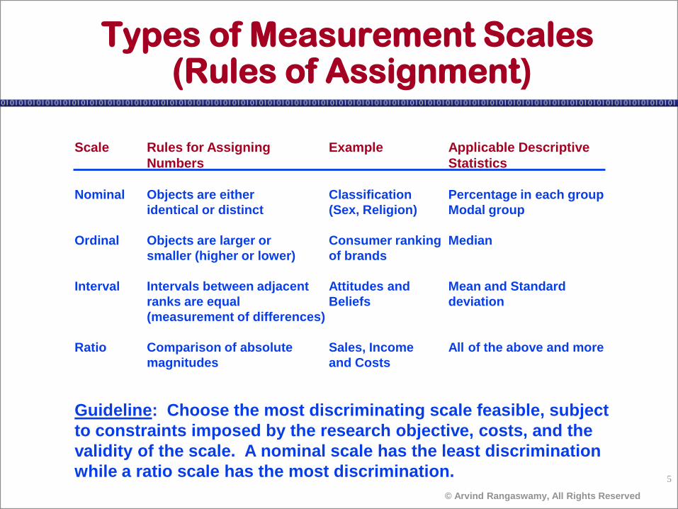
Scale Rules for Assigning Example Applicable Descriptive

Numbers Statistics

Nominal Objects are either Classification Percentage in each group

identical or distinct (Sex, Religion) Modal group

Ordinal Objects are larger or Consumer ranking Median

smaller (higher or lower) of brands

Interval Intervals between adjacent Attitudes and Mean and Standard

ranks are equal Beliefs deviation

(measurement of differences)

Ratio Comparison of absolute Sales, Income All of the above and more

magnitudes and Costs

Guideline: Choose the most discriminating scale feasible, subject

to constraints imposed by the research objective, costs, and the

validity of the scale. A nominal scale has the least discrimination

while a ratio scale has the most discrimination.

Types of Measurement Scales (Rules of Assignment)

6


Psychometric Approach to Preference Measurement

Create an axiomatic system to parsimoniously represent the laws by which individuals’ preferences for stimuli can be understood (Why is this useful?).

Develop a justifiable measurement procedure to create an index (e.g., an interval scale) such that the resulting scales denoting preferences can be mathematically manipulated to help us infer individuals’ preferences for unmeasured stimuli. (Why is this useful?)

7


Goals of Preference Measurement

A common framework to apply across multiple situations

Ability to generalize from study to market reality

Parsimony

Predictive ability (the “as if” concept)

8


Measuring Preference Structures of Interest to Marketers

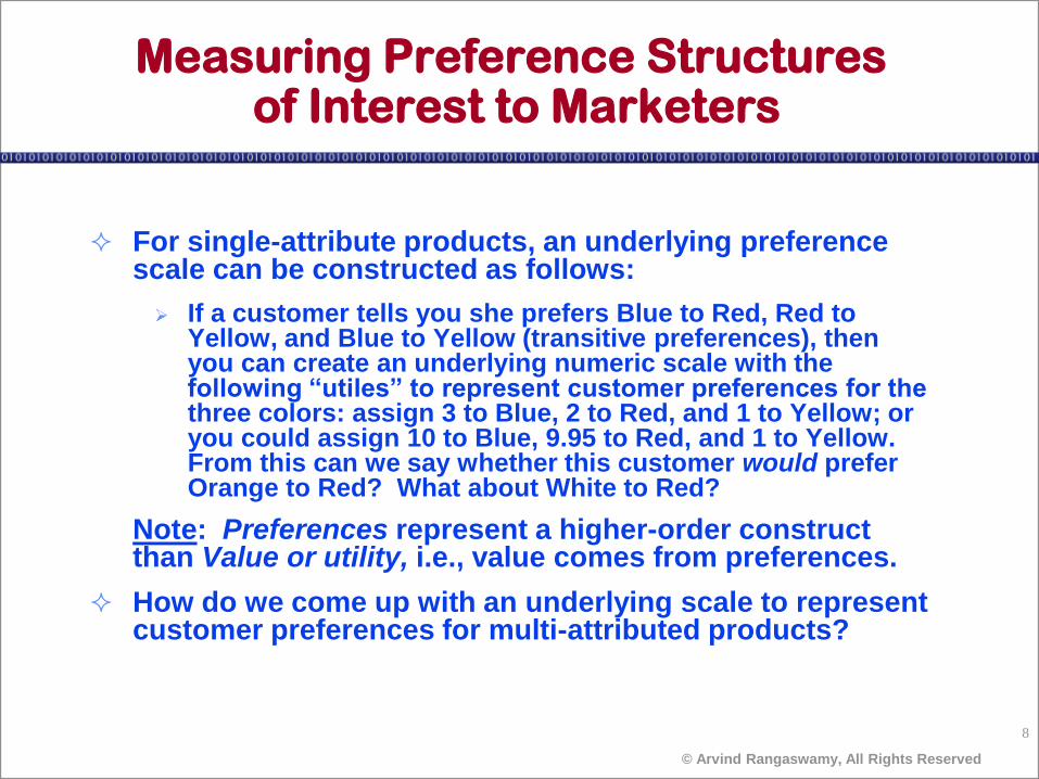
For single-attribute products, an underlying preference scale can be constructed as follows:

If a customer tells you she prefers Blue to Red, Red to Yellow, and Blue to Yellow (transitive preferences), then you can create an underlying numeric scale with the following “utiles” to represent customer preferences for the three colors: assign 3 to Blue, 2 to Red, and 1 to Yellow; or you could assign 10 to Blue, 9.95 to Red, and 1 to Yellow. From this can we say whether this customer would prefer Orange to Red? What about White to Red?

Note: Preferences represent a higher-order construct than Value or utility, i.e., value comes from preferences.

How do we come up with an underlying scale to represent customer preferences for multi-attributed products?

9


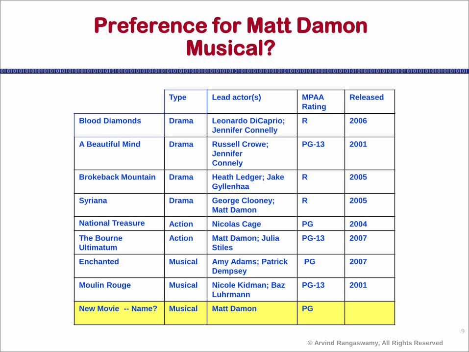
Preference for Matt Damon Musical?

Type Lead actor(s) MPAA

Rating

Released

Blood Diamonds Drama Leonardo DiCaprio;

Jennifer Connelly

R 2006

A Beautiful Mind Drama Russell Crowe;

Jennifer

Connely

PG-13 2001

Brokeback Mountain Drama Heath Ledger; Jake

Gyllenhaa

R 2005

Syriana Drama George Clooney;

Matt Damon

R 2005

National Treasure Action Nicolas Cage PG 2004

The Bourne

Ultimatum

Action Matt Damon; Julia

Stiles

PG-13 2007

Enchanted Musical Amy Adams; Patrick

Dempsey

PG 2007

Moulin Rouge Musical Nicole Kidman; Baz

Luhrmann

PG-13 2001

New Movie -- Name? Musical Matt Damon PG

10


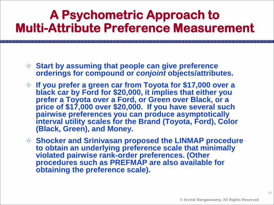
Start by assuming that people can give preference orderings for compound or conjoint objects/attributes.

If you prefer a green car from Toyota for $17,000 over a black car by Ford for $20,000, it implies that either you prefer a Toyota over a Ford, or Green over Black, or a price of $17,000 over $20,000. If you have several such pairwise preferences you can produce asymptotically interval utility scales for the Brand (Toyota, Ford), Color (Black, Green), and Money.

Shocker and Srinivasan proposed the LINMAP procedure to obtain an underlying preference scale that minimally violated pairwise rank-order preferences. (Other procedures such as PREFMAP are also available for obtaining the preference scale).

A Psychometric Approach to Multi-Attribute Preference Measurement

Discussion

Shocker and Srinivasan paper

12


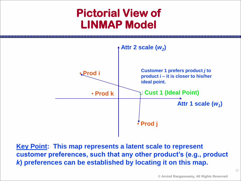
Pictorial View of LINMAP Model

Attr 1 scale (w1)

Attr 2 scale (w2)

• Prod i

• Prod j

Cust 1 (Ideal Point)

Customer 1 prefers product j to

product i – it is closer to his/her

ideal point.

Key Point: This map represents a latent scale to represent

customer preferences, such that any other product’s (e.g., product

k) preferences can be established by locating it on this map.

• Prod k

13


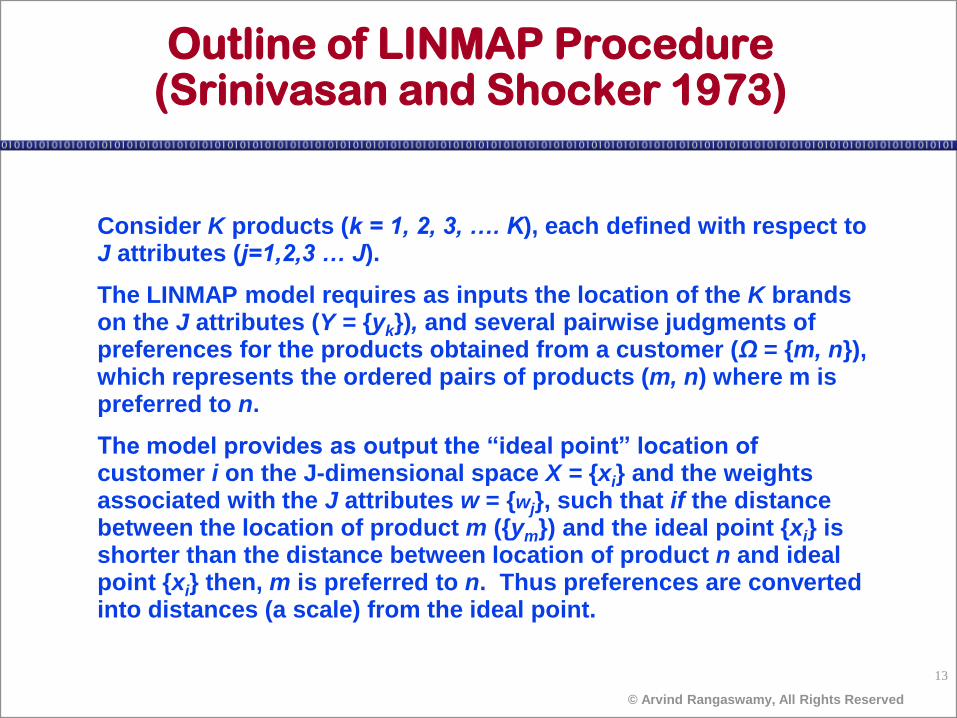
Outline of LINMAP Procedure (Srinivasan and Shocker 1973)

Consider K products (k = 1, 2, 3, …. K), each defined with respect to J attributes (j=1,2,3 … J).

The LINMAP model requires as inputs the location of the K brands on the J attributes (Y = {yk}), and several pairwise judgments of preferences for the products obtained from a customer (Ω = {m, n}), which represents the ordered pairs of products (m, n) where m is preferred to n.

The model provides as output the “ideal point” location of customer i on the J-dimensional space X = {xi} and the weights associated with the J attributes w = {wj}, such that if the distance between the location of product m ({ym}) and the ideal point {xi} is shorter than the distance between location of product n and ideal point {xi} then, m is preferred to n. Thus preferences are converted into distances (a scale) from the ideal point.

14


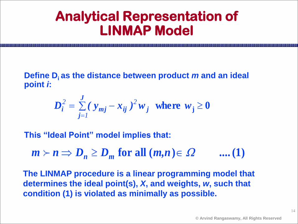
Analytical Representation of LINMAP Model

Define Di as the distance between product m and an ideal point i:

This “Ideal Point” model implies that:

0 where j

ww)xy(DJ

jjijmji

1

22

(1) .... )( allfor m,nDDnm mn

The LINMAP procedure is a linear programming model that

determines the ideal point(s), X, and weights, w, such that

condition (1) is violated as minimally as possible.

15


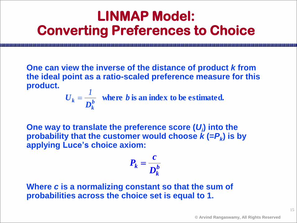
LINMAP Model: Converting Preferences to Choice

One can view the inverse of the distance of product k from the ideal point as a ratio-scaled preference measure for this product.

One way to translate the preference score (Ui) into the probability that the customer would choose k (=Pk) is by applying Luce’s choice axiom:

Where c is a normalizing constant so that the sum of probabilities across the choice set is equal to 1.

estimated. be toindex an is where bD

Ubk

k

1

bk

kD

cP

16


Some Issues Associated with Preference Measurement

Preference orderings provided by consumers did not always satisfy transitivity requirements.

Consumers did not always choose the products they preferred the most.

17


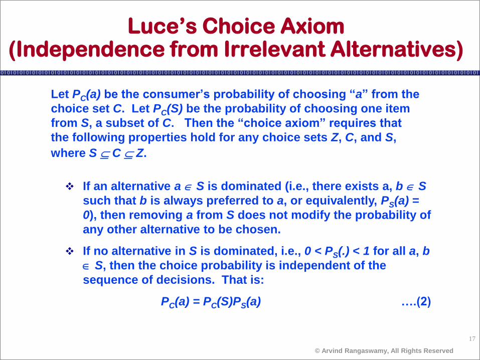
Let PC(a) be the consumer’s probability of choosing “a” from the

choice set C. Let PC(S) be the probability of choosing one item

from S, a subset of C. Then the “choice axiom” requires that

the following properties hold for any choice sets Z, C, and S,

where S C Z.

Luce’s Choice Axiom (Independence from Irrelevant Alternatives)

If an alternative a S is dominated (i.e., there exists a, b S

such that b is always preferred to a, or equivalently, PS(a) =

0), then removing a from S does not modify the probability of

any other alternative to be chosen.

If no alternative in S is dominated, i.e., 0 < PS(.) < 1 for all a, b

S, then the choice probability is independent of the

sequence of decisions. That is:

PC(a) = PC(S)PS(a) ….(2)

18


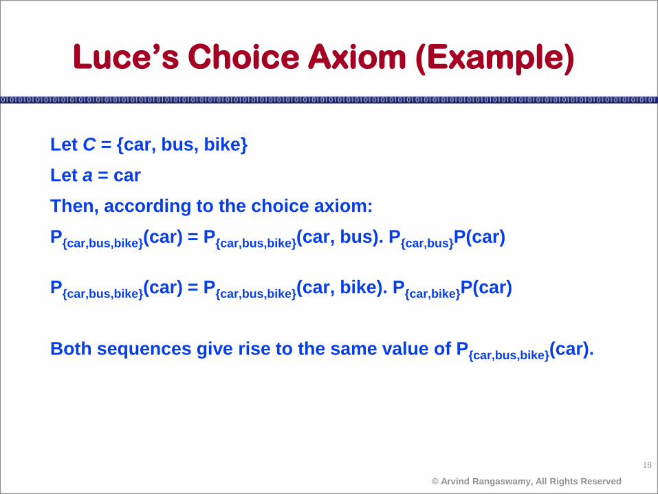
Luce’s Choice Axiom (Example)

Let C = {car, bus, bike}

Let a = car

Then, according to the choice axiom:

P{car,bus,bike}(car) = P{car,bus,bike}(car, bus). P{car,bus}P(car)

P{car,bus,bike}(car) = P{car,bus,bike}(car, bike). P{car,bike}P(car)

Both sequences give rise to the same value of P{car,bus,bike}(car).

19


Luce Choice Axiom

Luce has shown that (2) is a necessary and sufficient condition for the existence of a function U from C (the Real line), such that, for all S C, we have:

Think of U as a (fixed) utility function. It is easily seen that the result is equivalent to:

For any Choice sets S and T C, and for any alternatives a and b in S.

Sbb

aS

U

UaP )(

b

a

T

T

S

S

U

U

bP

aP

bP

aP

)(

)(

)(

)(

20


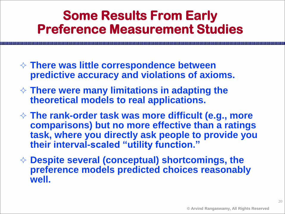
Some Results From Early Preference Measurement Studies

There was little correspondence between predictive accuracy and violations of axioms.

There were many limitations in adapting the theoretical models to real applications.

The rank-order task was more difficult (e.g., more comparisons) but no more effective than a ratings task, where you directly ask people to provide you their interval-scaled “utility function.”

Despite several (conceptual) shortcomings, the preference models predicted choices reasonably well.

21


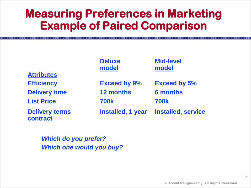
Measuring Preferences in Marketing Example of Paired Comparison

Deluxe Mid-level model model Attributes

Efficiency Exceed by 9% Exceed by 5%

Delivery time 12 months 6 months

List Price 700k 700k

Delivery terms Installed, 1 year Installed, service contract

Which do you prefer?

Which one would you buy?

22


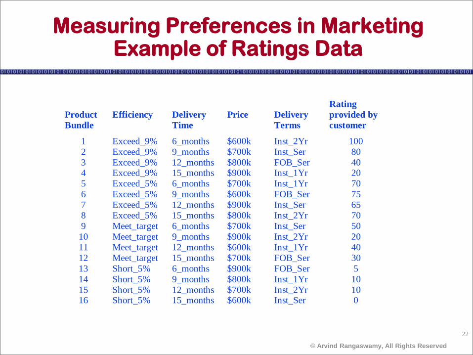
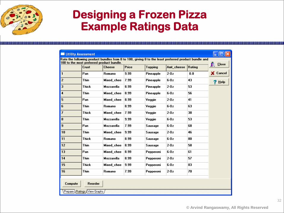
Measuring Preferences in Marketing Example of Ratings Data

Product

Bundle

Efficiency

Delivery

Time

Price

Delivery

Terms

Rating

provided by

customer

1 Exceed_9% 6_months $600k Inst_2Yr 100

2 Exceed_9% 9_months $700k Inst_Ser 80

3 Exceed_9% 12_months $800k FOB_Ser 40 4 Exceed_9% 15_months $900k Inst_1Yr 20


6 Exceed_5% 9_months $600k FOB_Ser 75

7 Exceed_5% 12_months $900k Inst_Ser 65


9 Meet_target 6_months $700k Inst_Ser 50

10 Meet_target 9_months $900k Inst_2Yr 20

11 Meet_target 12_months $600k Inst_1Yr 40

12 Meet_target 15_months $700k FOB_Ser 30

13 Short_5% 6_months $900k FOB_Ser 5

14 Short_5% 9_months $800k Inst_1Yr 10

15 Short_5% 12_months $700k Inst_2Yr 10 16 Short_5% 15_months $600k Inst_Ser 0

23


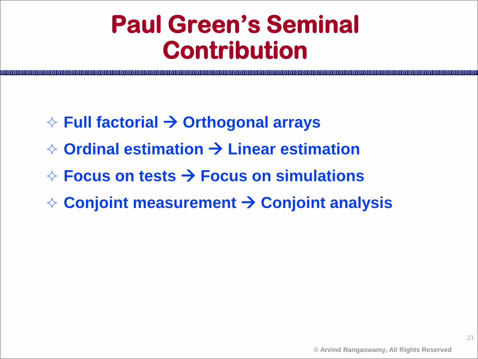
Paul Green’s Seminal Contribution

Full factorial Orthogonal arrays

Ordinal estimation Linear estimation

Focus on tests Focus on simulations

Conjoint measurement Conjoint analysis

24


Conjoint Measurement: Determining Importance of Attributes by Measuring Preferences

The basic assumption of Conjoint measurement is that customers cannot reliably express how they weight separate features of a product (or any other entity) in forming their preferences. However, we can infer the relative weights by asking for their evaluations (or choices) of alternate product concepts through a structured process (same idea in LINMAP).

25


Provides numerical values associated

with:

the relative importance that customers

attach to the attributes of a product

category

The value (utility or part-worth) provided

to customers by each potential feature

(attribute option) of an offering

Helps identify offering design(s) that

maximize market share or other

indices of performance.

What Does Conjoint Analysis Do?

26


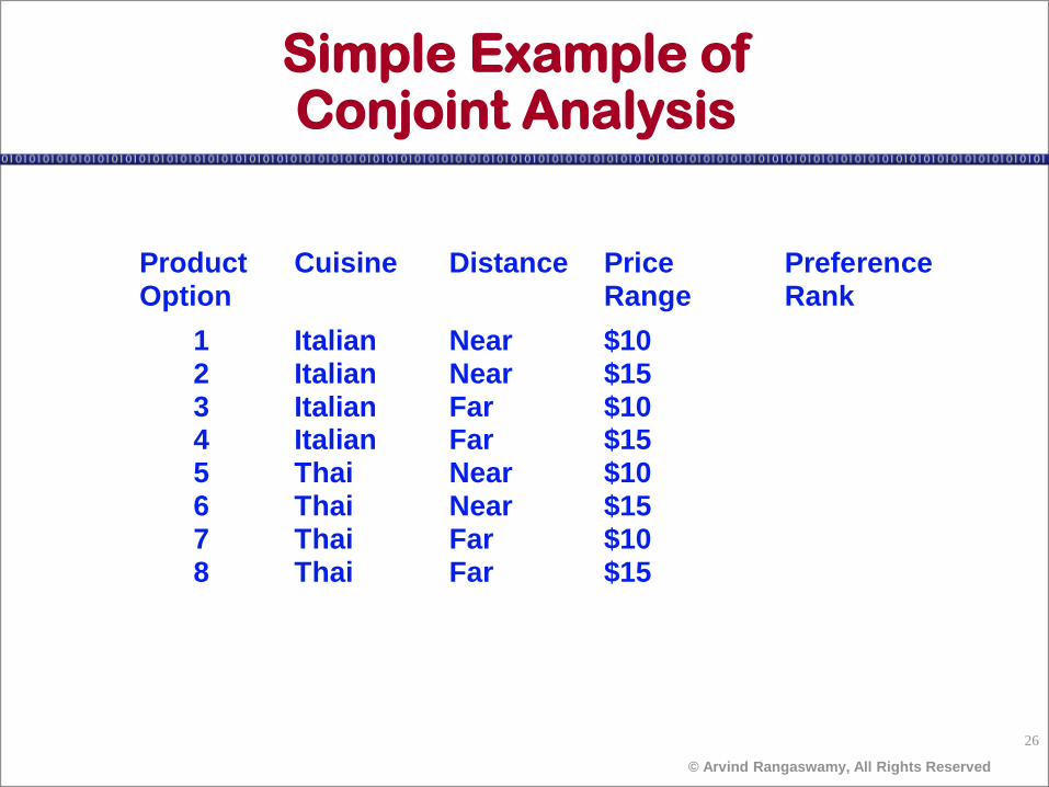
Product Option

Cuisine Distance Price Range

Preference Rank

1 Italian Near $10 2 Italian Near $15 3 Italian Far $10 4 Italian Far $15 5 Thai Near $10 6 Thai Near $15 7 Thai Far $10 8 Thai Far $15

Simple Example of Conjoint Analysis

27


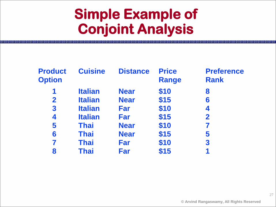
Simple Example of Conjoint Analysis

Product Option

Cuisine Distance Price Range

Preference Rank

1 Italian Near $10 8 2 Italian Near $15 6 3 Italian Far $10 4 4 Italian Far $15 2 5 Thai Near $10 7 6 Thai Near $15 5 7 Thai Far $10 3 8 Thai Far $15 1

28


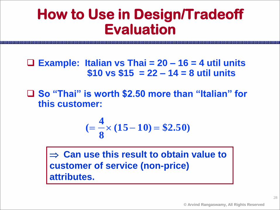
Example: Italian vs Thai = 20 – 16 = 4 util units $10 vs $15 = 22 – 14 = 8 util units

So “Thai” is worth $2.50 more than “Italian” for this customer: )50.2$)1015(

8

4(

Can use this result to obtain value to

customer of service (non-price)

attributes.

How to Use in Design/Tradeoff Evaluation

29


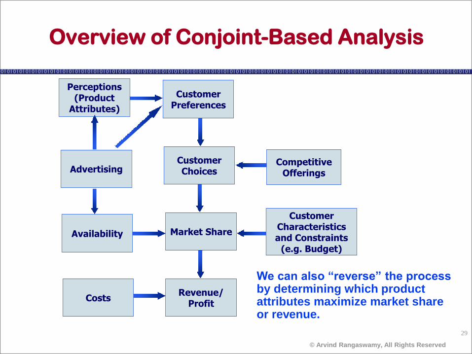
Overview of Conjoint-Based Analysis

Perceptions (Product

Attributes)

Customer Preferences

Advertising

Customer Characteristics and Constraints

(e.g. Budget)

Revenue/ Profit

Market Share

Customer Choices

Costs

Availability

Competitive Offerings

We can also “reverse” the process by determining which product attributes maximize market share or revenue.

30


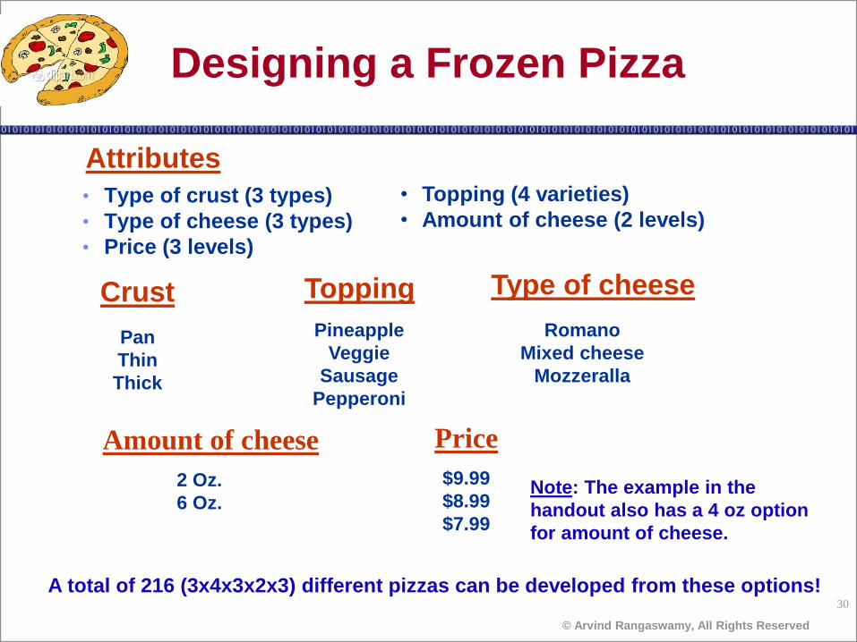
• Type of crust (3 types)

• Type of cheese (3 types)

• Price (3 levels)

Attributes • Topping (4 varieties)

• Amount of cheese (2 levels)

A total of 216 (3x4x3x2x3) different pizzas can be developed from these options!

Crust Topping Type of cheese

Pan

Thin

Thick

Pineapple

Veggie

Sausage

Pepperoni

Romano

Mixed cheese

Mozzeralla

Amount of cheese Price

2 Oz.

6 Oz.

$9.99

$8.99

$7.99

Designing a Frozen Pizza

Note: The example in the

handout also has a 4 oz option

for amount of cheese.

31


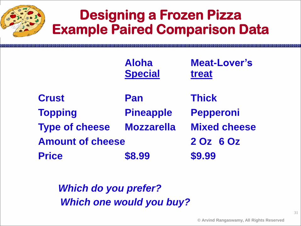
Aloha Meat-Lover’s Special treat

Crust Pan Thick

Topping Pineapple Pepperoni

Type of cheese Mozzarella Mixed cheese

Amount of cheese 2 Oz 6 Oz

Price $8.99 $9.99

Which do you prefer?

Which one would you buy?

Designing a Frozen Pizza Example Paired Comparison Data

32


Designing a Frozen Pizza Example Ratings Data

33


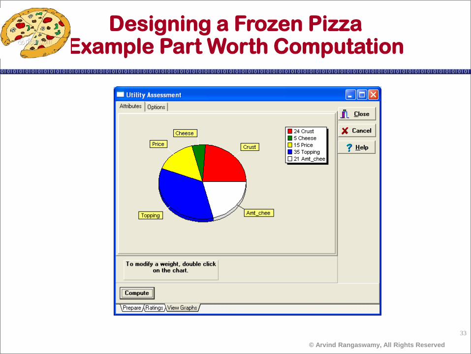
Designing a Frozen Pizza Example Part Worth Computation

34


Designing a Frozen Pizza Example Part Worth Computation

35


U(P) =S S ijxij

k

i=1

m

j=1

P: A particular product/concept of interest

U(P): The utility associated with product P

ij: Utility associated with the j th level (j = 1, 2, 3...kj) on

the i th attribute (referred to as part-worth)

kj: Number of levels of attribute i

m: Number of attributes

xij: 1 if the j th level of the i th attribute is present in

product P, 0 otherwise

Conjoint Utility Computations

j

Note: Once part-worths (ij) are determined, utilities can be computed (i.e.,

numbers can be assigned on the measurement scale) even for products not rated

by the customers.

36


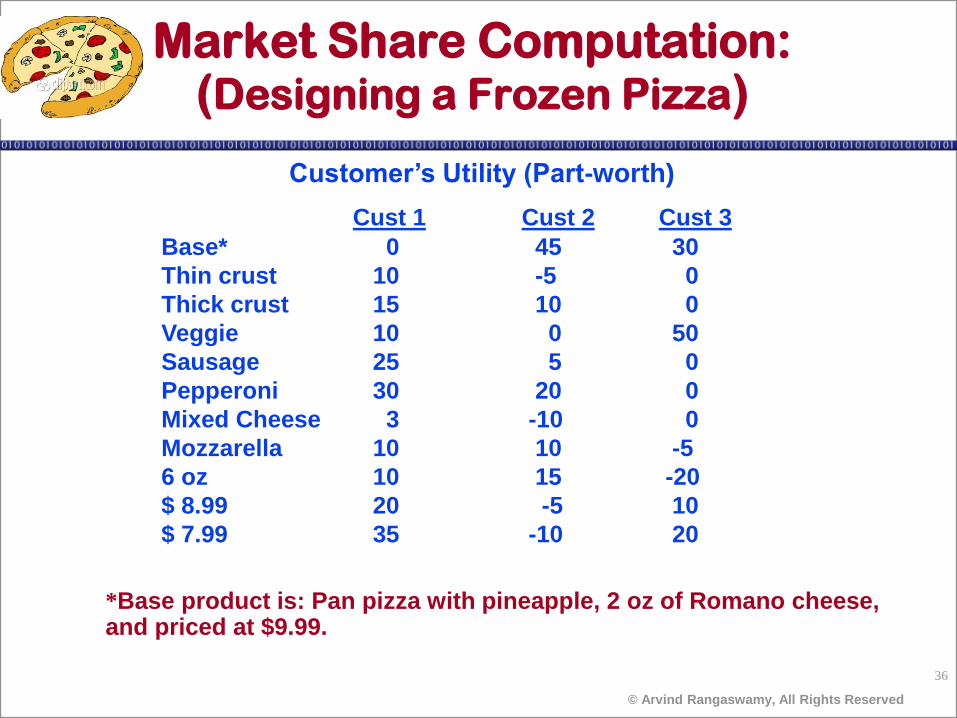
Market Share Computation: (Designing a Frozen Pizza)

Cust 1 Cust 2 Cust 3

Base* 0 45 30

Thin crust 10 -5 0

Thick crust 15 10 0

Veggie 10 0 50

Sausage 25 5 0

Pepperoni 30 20 0

Mixed Cheese 3 -10 0

Mozzarella 10 10 -5

6 oz 10 15 -20

$ 8.99 20 -5 10

$ 7.99 35 -10 20

Customer’s Utility (Part-worth)

*Base product is: Pan pizza with pineapple, 2 oz of Romano cheese, and priced at $9.99.

37


Define the competitive set – this is the set of products from which customers in the target segment make their choices. Some of them may be existing products and, others concepts being evaluated. We denote this set of products as P1, P2,...PN.

Select Choice rule

Single choice model

Share of preference model

Logit choice model

Other rules

Market Share and Revenue Share Forecasts

38


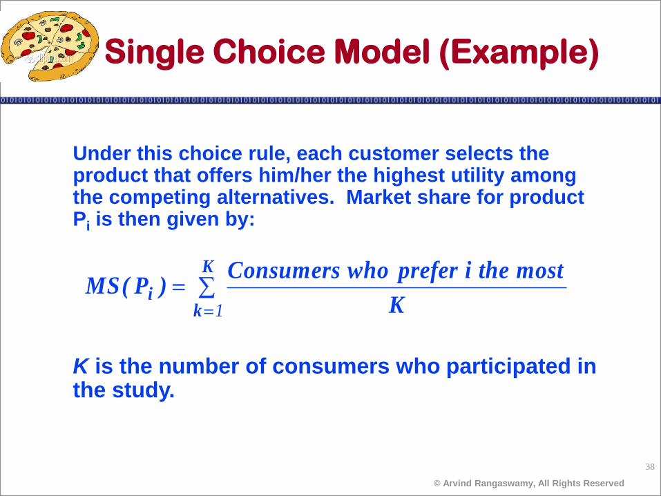
Single Choice Model (Example)

MS PConsumers who prefer i the most

Ki

k

K

( ) 1

Under this choice rule, each customer selects the product that offers him/her the highest utility among the competing alternatives. Market share for product Pi is then given by:

K is the number of consumers who participated in the study.

39


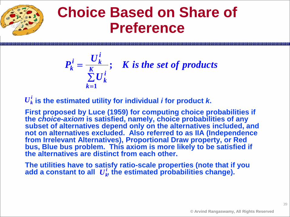
Choice Based on Share of Preference

is the estimated utility for individual i for product k.

First proposed by Luce (1959) for computing choice probabilities if the choice-axiom is satisfied, namely, choice probabilities of any subset of alternatives depend only on the alternatives included, and not on alternatives excluded. Also referred to as IIA (Independence from Irrelevant Alternatives), Proportional Draw property, or Red bus, Blue bus problem. This axiom is more likely to be satisfied if the alternatives are distinct from each other.

The utilities have to satisfy ratio-scale properties (note that if you add a constant to all , the estimated probabilities change).

productsofsettheisK

U

UP

K

k

ik

iki

k ;

1

ikU

ikU

40


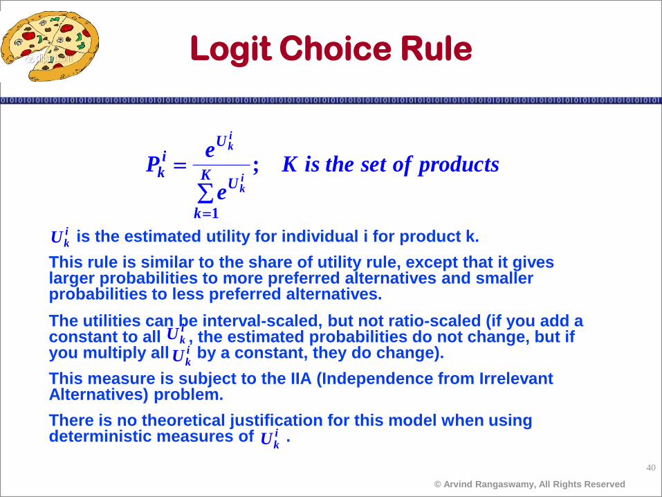
Logit Choice Rule

is the estimated utility for individual i for product k.

This rule is similar to the share of utility rule, except that it gives larger probabilities to more preferred alternatives and smaller probabilities to less preferred alternatives.

The utilities can be interval-scaled, but not ratio-scaled (if you add a constant to all , the estimated probabilities do not change, but if you multiply all by a constant, they do change).

This measure is subject to the IIA (Independence from Irrelevant Alternatives) problem.

There is no theoretical justification for this model when using deterministic measures of .

productsofsettheisK

e

eP

K

k

U

Ui

k ik

ik

;

1

ikU

ikU

ikU

ikU

41


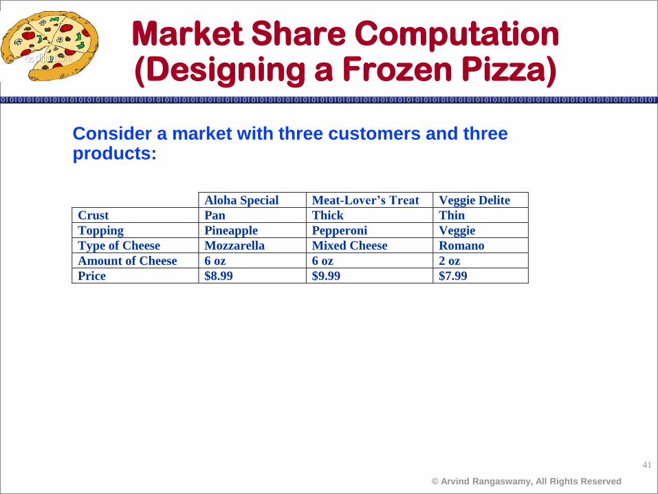
Market Share Computation (Designing a Frozen Pizza)

Consider a market with three customers and three products:

Aloha Special Meat-Lover’s Treat Veggie Delite

Crust Pan Thick Thin

Topping Pineapple Pepperoni Veggie

Type of Cheese Mozzarella Mixed Cheese Romano

Amount of Cheese 6 oz 6 oz 2 oz

Price $8.99 $9.99 $7.99

42


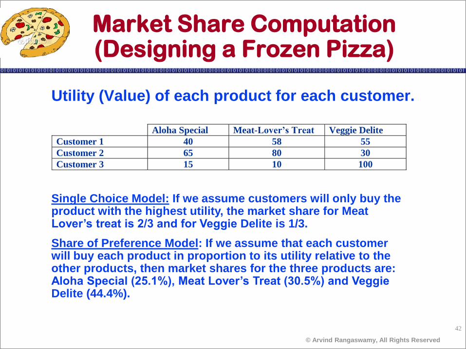
Market Share Computation (Designing a Frozen Pizza)

Utility (Value) of each product for each customer.

Aloha Special Meat-Lover’s Treat Veggie Delite

Customer 1 40 58 55

Customer 2 65 80 30

Customer 3 15 10 100

Single Choice Model: If we assume customers will only buy the product with the highest utility, the market share for Meat Lover’s treat is 2/3 and for Veggie Delite is 1/3.

Share of Preference Model: If we assume that each customer will buy each product in proportion to its utility relative to the other products, then market shares for the three products are: Aloha Special (25.1%), Meat Lover’s Treat (30.5%) and Veggie Delite (44.4%).

43


Preference Heterogeneity

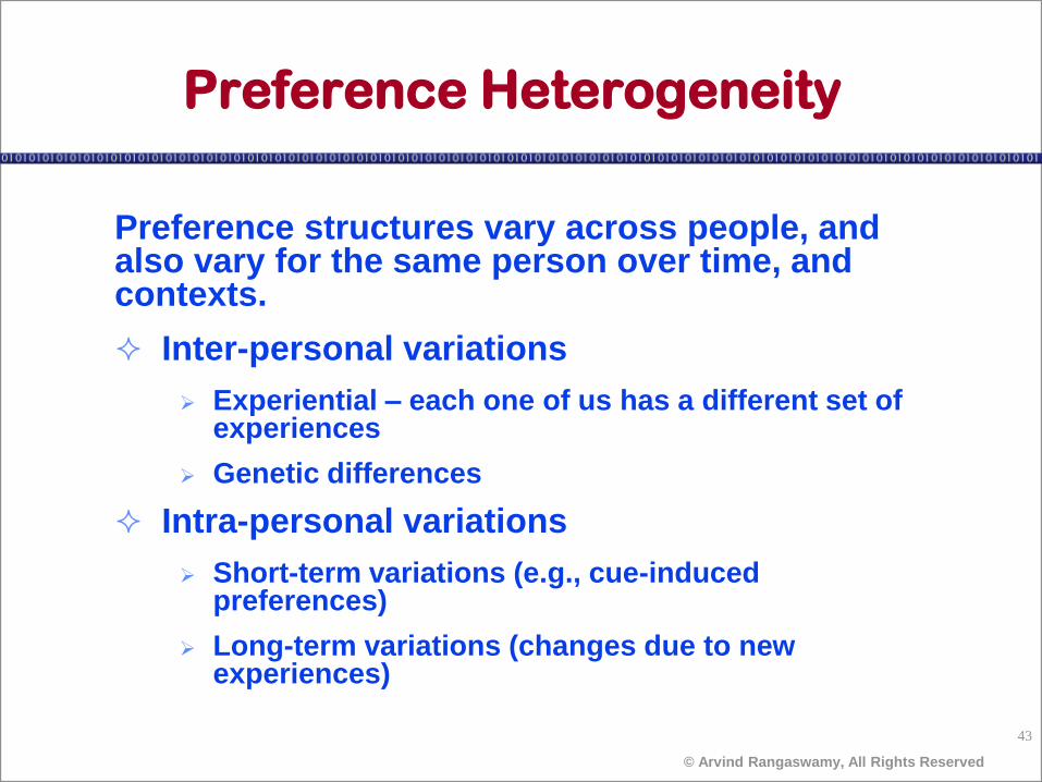
Preference structures vary across people, and also vary for the same person over time, and contexts.

Inter-personal variations

Experiential – each one of us has a different set of experiences

Genetic differences

Intra-personal variations

Short-term variations (e.g., cue-induced preferences)

Long-term variations (changes due to new experiences)

44


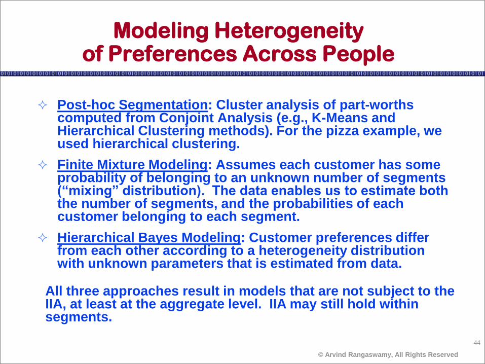
Modeling Heterogeneity of Preferences Across People

Post-hoc Segmentation: Cluster analysis of part-worths computed from Conjoint Analysis (e.g., K-Means and Hierarchical Clustering methods). For the pizza example, we used hierarchical clustering.

Finite Mixture Modeling: Assumes each customer has some probability of belonging to an unknown number of segments (“mixing” distribution). The data enables us to estimate both the number of segments, and the probabilities of each customer belonging to each segment.

Hierarchical Bayes Modeling: Customer preferences differ from each other according to a heterogeneity distribution with unknown parameters that is estimated from data.

All three approaches result in models that are not subject to the IIA, at least at the aggregate level. IIA may still hold within segments.

45


Finite Mixture Modeling Example (Latent Class Segmentation)

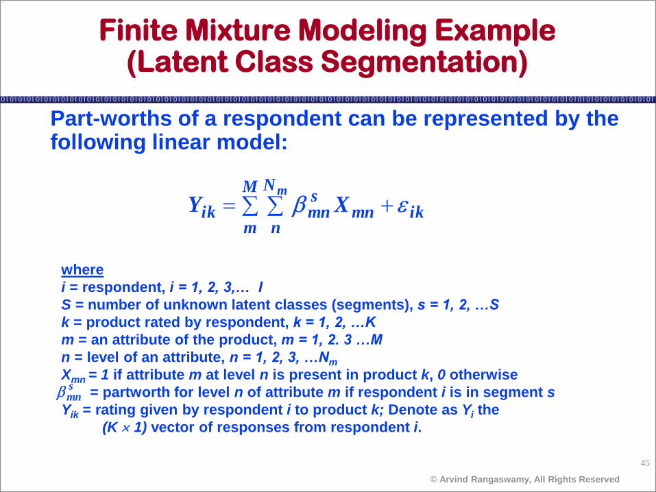
Part-worths of a respondent can be represented by the following linear model:

ik

M

m

N

nmn

smnik

m

XY

where

i = respondent, i = 1, 2, 3,… I

S = number of unknown latent classes (segments), s = 1, 2, …S

k = product rated by respondent, k = 1, 2, …K

m = an attribute of the product, m = 1, 2. 3 …M

n = level of an attribute, n = 1, 2, 3, …Nm

Xmn = 1 if attribute m at level n is present in product k, 0 otherwise

= partworth for level n of attribute m if respondent i is in segment s

Yik = rating given by respondent i to product k; Denote as Yi the

(K 1) vector of responses from respondent i.

smn

46



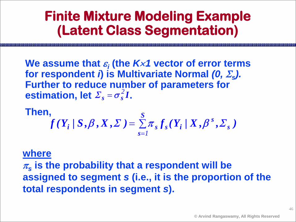
We assume that i (the K1 vector of error terms for respondent i) is Multivariate Normal (0, Ss). Further to reduce number of parameters for estimation, let .

Then,

Iss2S

),,X|Y(f),X,,S|Y(f ss

is

S

ssi SS

1

where

s is the probability that a respondent will be

assigned to segment s (i.e., it is the proportion of the

total respondents in segment s).

47



The parameters can be estimated by maximizing Log Likelihood as follows (What assumption are we making here?)

),,X|Y(fLnLLn s

sI

i

S

siss S

1 1

algorithm) EM (e.g., methods numerical via and, , estimate We s

s ˆˆ,ˆS S

Typically, the optimal number of segments are

chosen by minimizing a criterion called BIC – the

lower the better.

48



To determine the part-worths for each individual, we do the following computations.

In practical segmentation studies, respondent i can be assigned to the segment to which he/she has the highest probability of belonging.

S

s

si

S

ss

siss

ss

iss

ˆ)si(Pˆ

S,...,s;

)ˆ,ˆ,X|Y(fˆ

)ˆ,ˆ,X|Y(fˆ)si(P

1

1

21

S

S

49


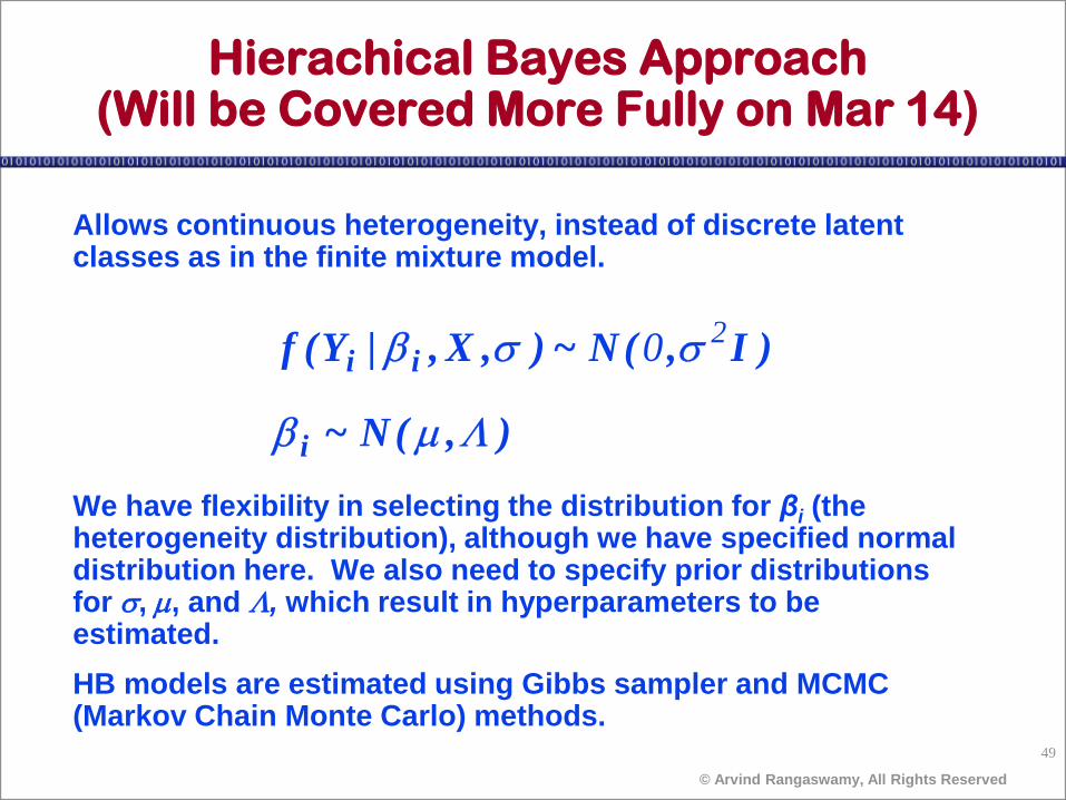
Hierachical Bayes Approach (Will be Covered More Fully on Mar 14)

Allows continuous heterogeneity, instead of discrete latent classes as in the finite mixture model.

We have flexibility in selecting the distribution for βi (the heterogeneity distribution), although we have specified normal distribution here. We also need to specify prior distributions for , , and , which result in hyperparameters to be estimated.

HB models are estimated using Gibbs sampler and MCMC (Markov Chain Monte Carlo) methods.

),(N~

)I,(N~),X,|Y(f

i

ii

20

mktg 555: marketing models - personal.psu.edu · 1 © arvind rangaswamy, all rights reserved mktg...

Documents