9/9/2011 Classical Control 1

MM11 Root Locus Design MethodMM11 Root Locus Design Method

Reading material: FC pp.270-328Reading material: FC pp.270-328

9/9/2011 Classical Control 2

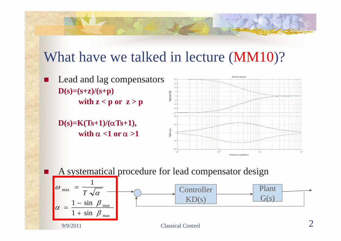
What have we talked in lecture (MM10)? Lead and lag compensators

D(s)=(s+z)/(s+p) with z < p or z > p

D(s)=K(Ts+1)/(Ts+1), with <1 or >1

A systematical procedure for lead compensator design

max

max

max

sin1sin1

1

T Controller

KD(s)PlantG(s)

9/9/2011 Classical Control 3

Goals for this lecture (MM11) What’s root locus?

Definition features

How to sketch a root locus? Manually Matlab - rlocus()

How to use root locus for control design?

9/9/2011 Classical Control 4

Control system design for a satellite tracking antenna

Design specifications: Overshoot to a step input less than 16%; Settling time to 2% to be less than 10

sec.; Tracking error to a ramp input of slope

0.01rad/sec to be less than 0.01rad; Sampling time to give at at least 10

samples in a rise time.

Illustrative Example: Antenna Control from MM10?

9/9/2011 Classical Control 5

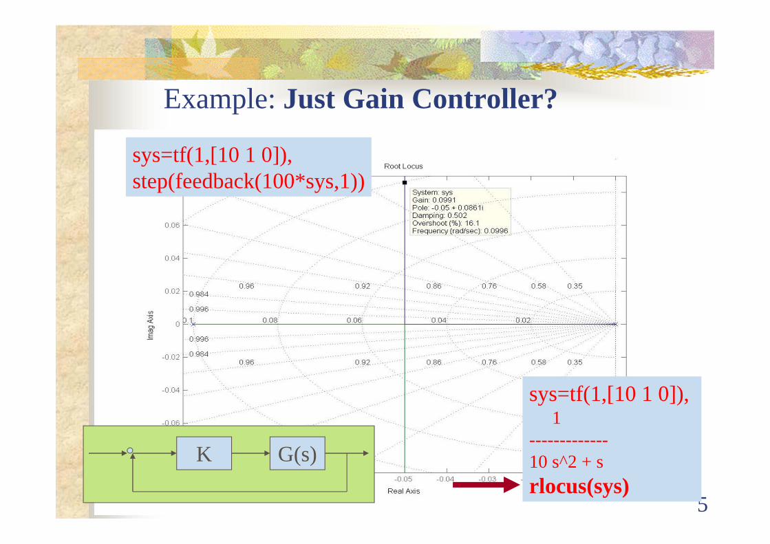
G(s)K

sys=tf(1,[10 1 0]), 1

-------------10 s^2 + srlocus(sys)

Example: Just Gain Controller?

sys=tf(1,[10 1 0]), step(feedback(100*sys,1))

9/9/2011 Classical Control 6

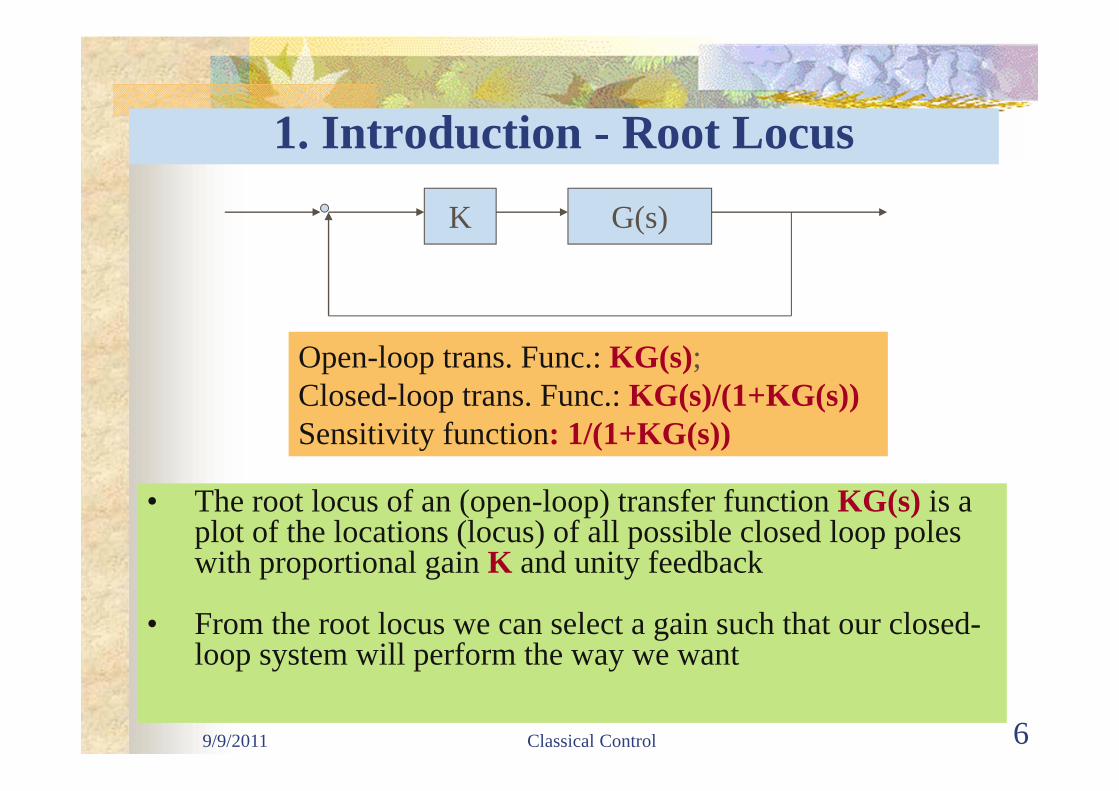
1. Introduction - Root Locus

• The root locus of an (open-loop) transfer function KG(s) is a plot of the locations (locus) of all possible closed loop poles with proportional gain K and unity feedback

• From the root locus we can select a gain such that our closed-loop system will perform the way we want

G(s)K

Open-loop trans. Func.: KG(s); Closed-loop trans. Func.: KG(s)/(1+KG(s))Sensitivity function: 1/(1+KG(s))

9/9/2011 Classical Control 7

Root Locus: Effects of Poles

2

2

..

2.

2

2

1,::

)(1)sin(1

)(2

)(

ndnn

dtn

nn

n

quencynaturalfreratiodamping

ttethss

sH

2

1/

1,

10,

6.46.4

8.1

2

ndd

p

p

ns

nr

t

eM

t

t

9/9/2011 Classical Control 8

Root Locus: Definition Root locus is the set of vaues of s for which the follwing

equation holds for some positive real vaue of K1+KG(s)=0

Example1:G(s)=1/s(s+1)

Example2:G(s)=1/s(s+c)

9/9/2011 Classical Control 9

How to Sketch a Root Locus? Principles: The root locus must have n branches, where n is the number

of poles of G(s)

Each branch starts at a pole of G(s) and goes to a zero of G(s)

If G(s) has more poles than zeros: m < n, we say that G(s) has zeros at infinity, i.e., there are n-m number of branches of the root locus that go to infinity (asymptotes)

9/9/2011 Classical Control 10

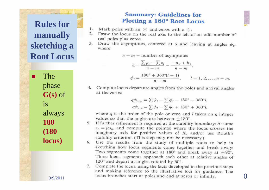
Rules for manually

sketching a Root Locus

The phase G(s) of is always 180 (180 locus)

9/9/2011 Classical Control 11

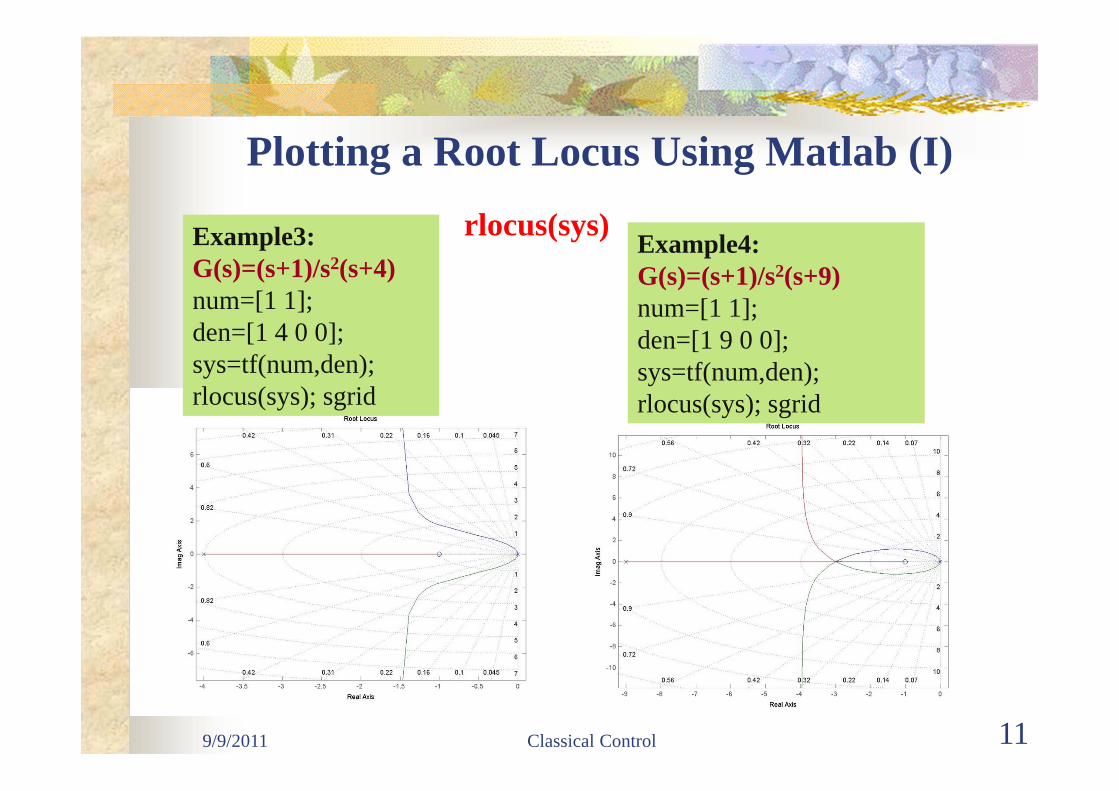
rlocus(sys)

Plotting a Root Locus Using Matlab (I)

Example4:G(s)=(s+1)/s2(s+9)num=[1 1]; den=[1 9 0 0]; sys=tf(num,den); rlocus(sys); sgrid

Example3:G(s)=(s+1)/s2(s+4)num=[1 1]; den=[1 4 0 0]; sys=tf(num,den); rlocus(sys); sgrid

9/9/2011 Classical Control 12

Example5:G(s)=(s+1)/s2(s+12)num=[1 1]; den=[1 12 0 0]; sys=tf(num,den); rlocus(sys); sgrid

Example6:G(s)=1/[s(s+2)[(s+1)2+4]]num=[1]; den=conv([1 2 0],[1 2 5]); sys=tf(num,den); rlocus(sys); sgrid

rlocus(sys)

Plotting a Root Locus Using Matlab (II)

9/9/2011 Classical Control 13

Control Design Using Root Locus (I) Objective: select a

particular value of K that will meet the specifications for static and dynamic

1+KG(s)=0

Magnitude condition:K=1/|G(s)|

9/9/2011 Classical Control 14

Control Design Using Root Locus (II) Command sgrid(Zeta,Wn) to plot lines of constant

damping ratio Zeta and natural frequency Wn

Example: an overshoot less than 5% (which means a damping ratio greater than 0.7) and a rise time of 1 second (which means a natural frequency Wn greater than 1.8). zeta=0.7; Wn=1.8; sgrid(zeta, Wn)

9/9/2011 Classical Control 15

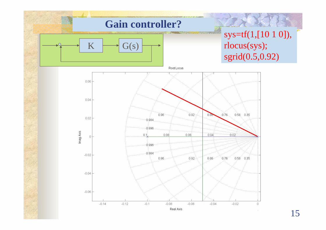
G(s)Ksys=tf(1,[10 1 0]), rlocus(sys); sgrid(0.5,0.92)

Gain controller?

9/9/2011 Classical Control 16

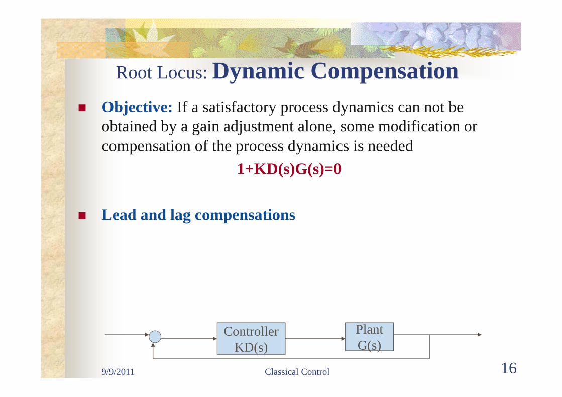
Root Locus: Dynamic Compensation Objective: If a satisfactory process dynamics can not be

obtained by a gain adjustment alone, some modification or compensation of the process dynamics is needed

1+KD(s)G(s)=0

Lead and lag compensations

ControllerKD(s)

PlantG(s)

9/9/2011 Classical Control 17

Lead Compensation (I) Lead compensation: acts mainly to lower rise time and

decrease the transient overshoot: D(s)=(s+z)/(s+p) with z < p

It moves the locus to the left and typically improves the system damping

Zero and pole selections (empirical rule) The zero is placed in the neighborhood of the

closed-loop n as determined by rise-time or settling-time requirements

The pole is located at s distance 3 to 20 times the value of the zero location

9/9/2011 Classical Control 18

Lead Compensation (II)

Example: G(s)=K/s(s+1)D1(s)=s+2; D2(s)=(s+2)/(s+20)D3(s)=(s+2)/(s+10)

9/9/2011 Classical Control 19

Lead Compenstor: Antenna Control Example

Step 1: Select the lead compensator as: D(s)=(s+0.92)/(s+10)sysDG=tf(1,[10 1 0])*tf([1 0.92],[1 10]);

Step 2: Draw the rootlocus to determine the Krlocus(sysDG), sgrid(0.5,0.92)

Step 3: Construct the close-loop system and check the requirements are satisfied or not

syscl=feedback(K*sysDG,1); figure; step(syscl), grid Step 4: If the requirements can not be satisfied, iterate the

design procedure

Do your design using the root locus method!

9/9/2011 Classical Control 20

Lag Compensation (I)Lag compensator acts mainly to improve the steady-state accuracy:

D(s)=(s+z)/(s+p) with z > p

Lag compensator approximates PI control

Zero and pole selection Select a pole near s=0, and also select the zero nearby, such

that the dipole does not significantly interfere the response The lag compensation usually degrades stability

9/9/2011 Classical Control 21

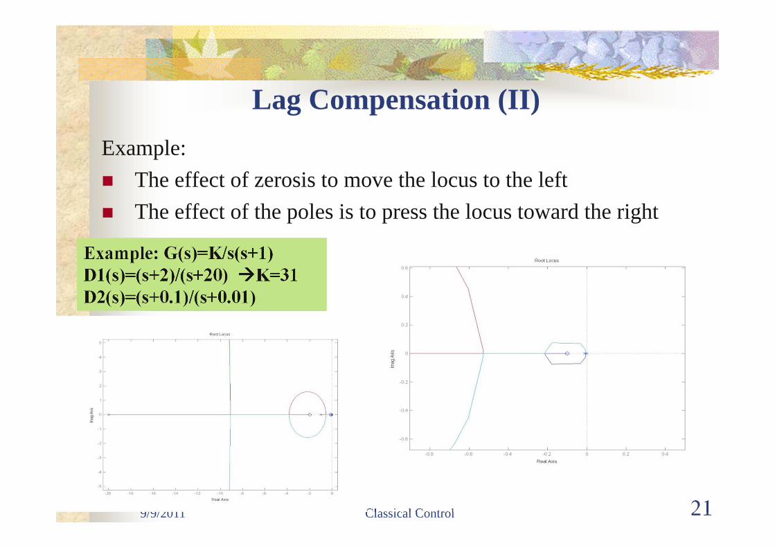
Lag Compensation (II)Example: The effect of zerosis to move the locus to the left The effect of the poles is to press the locus toward the right

Example: G(s)=K/s(s+1)D1(s)=(s+2)/(s+20) K=31D2(s)=(s+0.1)/(s+0.01)

9/9/2011 Classical Control 22

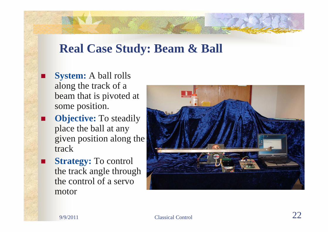
Real Case Study: Beam & Ball

System: A ball rollsalong the track of a beam that is pivoted at some position.

Objective: To steadily place the ball at any given position along the track

Strategy: To control the track angle through the control of a servo motor

9/9/2011 Classical Control 23

Example: Open-Loop Analysism = 0.111; R = 0.015; g = -9.8; L = 1.0; d = 0.03; J = 9.99e-6; K=(m*g*d)/(L*(J/R^2+m));num = [-K]; den = [1 0 0];rlocus(num,den); sgrid(0.70, 1.9); axis([-5 5 -2 2])

9/9/2011 Classical Control 24

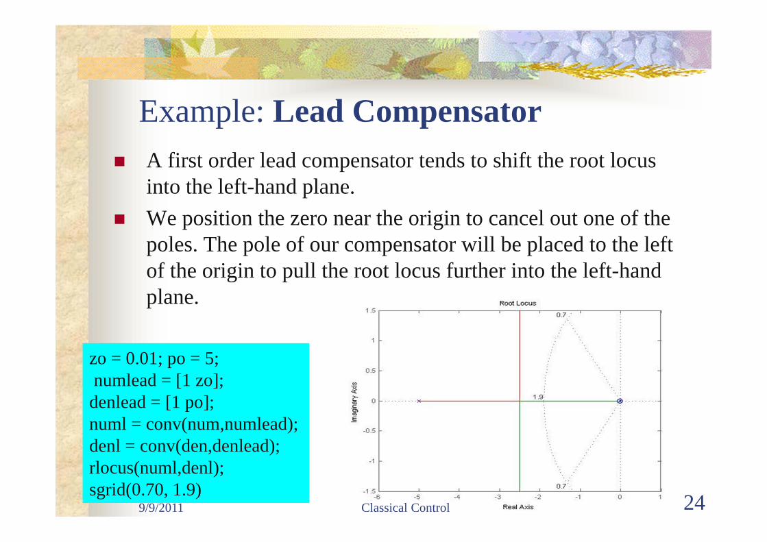
Example: Lead Compensator A first order lead compensator tends to shift the root locus

into the left-hand plane. We position the zero near the origin to cancel out one of the

poles. The pole of our compensator will be placed to the left of the origin to pull the root locus further into the left-hand plane.

zo = 0.01; po = 5;numlead = [1 zo]; denlead = [1 po]; numl = conv(num,numlead); denl = conv(den,denlead); rlocus(numl,denl); sgrid(0.70, 1.9)

9/9/2011 Classical Control 25

Example: Finding a Gain K [kc,poles]=rlocfind(numl,denl)

kc = 35.0253;numl2 = kc*numl; [numcl,dencl] = cloop(numl2,denl);t=0:0.01:5;figure step(1*numcl,dencl,t)

9/9/2011 Classical Control 26

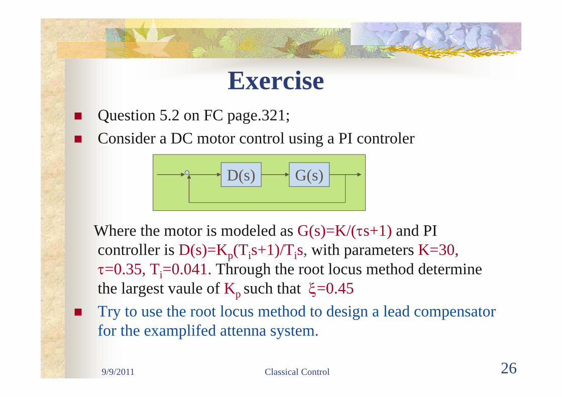
Exercise Question 5.2 on FC page.321; Consider a DC motor control using a PI controler

Where the motor is modeled as G(s)=K/(s+1) and PI controller is D(s)=Kp(Tis+1)/Tis, with parameters K=30, =0.35, Ti=0.041. Through the root locus method determine the largest vaule of Kp such that =0.45

Try to use the root locus method to design a lead compensator for the examplifed attenna system.

G(s)D(s)