mmuummaa pprroo - scienscope · company or services department to change the manual. in order to...

MMUUMMAA PPrroo

MMaannuuaall

Jan-2012

CONTENT 1. System Demand................................................................................................................ 3

1.1 Computer System Demand ................................................................................................... 3

1.2 Machine Software Demand .................................................................................................. 3

2 Install Drivers and Software ................................................................................................ 3

2.1 Install DH-HV1351UC Camera Driver ................................................................................ 3

2.2 Install USB Counter Card Driver .......................................................................................... 7

2.3 Install USB Lamp Driver .................................................................................................... 12

2.4 Install Software Key Driver ................................................................................................ 17

2.5 Install OVM Software ......................................................................................................... 19

2.6 Set Utility ............................................................................................................................ 22

3. Basic OVM Software Operation ....................................................................................... 24

3.1 Start OVM Software ........................................................................................................... 24

3.2 Image Calibration ............................................................................................................... 26

3.3 Close OVM Software .......................................................................................................... 27

4. OVM Software Window .................................................................................................. 28

4.1 OVM Software Window Introduction ................................................................................ 28

4.2 Main Menu .......................................................................................................................... 29

4.3 DRO Display ....................................................................................................................... 33

4.4 Measured Data List ............................................................................................................. 34

4.5 Measured Object List .......................................................................................................... 35

4.6 Top and bottom Light Control ............................................................................................ 36

4.7 Measuring Tool ................................................................................................................... 37

5. Image Measure ............................................................................................................... 57

5.1 Bottom Light to Measure .................................................................................................... 57

5.2 Top Light to Measure ......................................................................................................... 57

5.3 CCD Setup .......................................................................................................................... 57

5.5 Output setting ...................................................................................................................... 59

5.6 DRO Setting ........................................................................................................................ 59

5.7Live Image ........................................................................................................................... 60

5.8Capture Still Image .............................................................................................................. 60

6. Learning function and coordinate transfer .......................................................................... 61

6.1 Measuring request ............................................................................................................... 61

6.2 Coordinate establishment .................................................................................................... 65

6.3 Regression line .................................................................................................................... 69

6.4 SPC Control ........................................................................................................................ 71

6.5 Workpiece datum setting .................................................................................................... 73

7. Checking ........................................................................................................................ 80

7.1Quick Access ....................................................................................................................... 80

7.2 SPC ..................................................................................................................................... 91

7.3Graph Data ........................................................................................................................... 94

7.4 Focusing .............................................................................................................................. 96

3

1

NOTICE

Dear Customers:

Thanks very much for reading OVM software manual of vision measuring machines.

To ensure the safe and efficient use of this system, please read this manual carefully

before starting to operate and take good care.

In order to enable you to learn well for this OVM manual as soon as possible, we

prepared the manual for you specially. We try our best to make its presentation more

comprehensive and concise, from which you can get knowledge about the system

configuration, installation steps and operation methods. We strongly recommend you to

read carefully before use the product; this will help you to make a better use. If there are

operations which are not according to the manual, we will not assume responsibility for the

relevant losses.

The manual we introduced here is just fit for the OVM, and will not indicate the

actual configuration of software and hardware products and interfaces. Please get the

actual configuration from the packing list which is accompanied with the machines, and

note that the manual does not apply to other products models and configurations.

We have given our best efforts to try to avoid human errors and ensure the

information accurate and reliable in the manual, but inevitably there may be some errors

which were not found before printing, as well as those beyond our control, such as

omissions in printing, binding, distribution aspects. If there are, please contact our

company or services department to change the manual.

In order to enhance performance and reliability of the machine and parts, there may

be a little adjustments for the hardware or software configuration, so there is likely to cause

some inconsistency between the manual and the actual situation, but this does not affect

the machine use, if there is difference, please access to the actual product, or contact the

company or the relevant department for consultative services.

Thanks a lot for your kind cooperation and supports！

1

OVM is a powerful image-based measuring system whose major functions includes

geometric measuring and image measuring. The system is professional software for 2D

measuring. It is very simple to operate and is compatible with CAD/CAM or Microsoft

Word/Excel for result processing.

Some features of the system include:

1. Offering image measuring tools so that measuring point, line, arc, circle etc can be

quite simple

2. Powerful math calculating ability; able to remove rough edge so as to obtain

accurate measuring result

3. The measuring image and result can be directly displayed on the computer screen

4. Image tools offer quick work on 2D profile points scan

5. Using figure to display the measuring objects; the figure can be saved, printed or

changed into Microsoft WORD (*.doc), EXCEL (*.xls) or AUTOCAD (*. Dxf) file format

6. Able to do tolerance analysis, and effective quality test

7. The object-based design allows you do direct calculations on the work piece

8. Compatible in XP operating system

The system can be used in the following industries: 2D measuring, cell-phone,

automobile parts, wrist-watch, precise measuring, electron, mould, puncher, spring, screw,

props, plastics, rubber, stopping valve, camera, bicycle parts, PCB board, conductive

rubber, wire shelf, electronic part group.

2

How to use this manual?

This manual can be used for the edition above OVM.

A major characteristic of OVM is that it can do 2D measuring quickly. Considering

the 2D measuring process, we provide two means here to help you to shorten the time of

processing: one is to provide user-friendly interface in OVM; the other is to list in detail in

this manual various kinds of functions, working techniques of the system as well as all

possible questions that you may meet when use this system.

When you use the manual for the first time, you’d better browse the contents first to

get a quick view of all the information offered and then read the parts that you are

interested in. If you want to inquire about single function of the software, you can get to

the part by using the content.

3

1. System Demand OVM is a specialized system that combines software and hardware. Before installing

OVM system, it is strongly suggested that you should confirm in advance that your

computer can match the following minimum demands. Otherwise, the efficiency of the

system may be reduced.

1.1 Computer System Demand

CPU: Pentium grade or above ( Pentium Ⅳ or above suggest)

RAM- memory: 512MB at least ( 1G memory suggest)

HD- hard disk: at least 50MB surplus storage space

Independent graphics card

Printer- (optional equipment, but essential if you want to print the report data)

Operating system: Windows 7

32 bit color quality of the screen is needed, the 24” display screen resolution is

1920*1080

Import/Export device : USB Serial port X1 at least

1.2 Machine Software Demand

Professional vision measuring software: OVM version

DH-HV1351UC camera program driver

USB 2.0 counter card program driver

USB lamp4 program driver

OVM software key program driver

2 Install Drivers and Software

2.1 Install DH-HV1351UC Camera Driver

Connect DH-1351UC camera to computer, right-click “Computer--Manage”.

4

Open “Device Manager”, right-click” Unknown device”, and then choose “Update Driver

Software”.

Choose “Browse my computer for driver software”.

5

Browse this camera driver location which depends on your saved position, and then click

“Next” to installation.

Camera driver is installing. Because camera driver is not register in Windows system, so

you will see one prompt, and choose “Install this drive software anyway”.

6

Camera driver is installed successfully, click “Close” to finish.

Check DH-1351UC camera driver is installed successfully in “Device Manager”.

7

2.2 Install USB Counter Card Driver

Connect 3DFAMILY USB2.0 counter card to USB port of computer, right-click “my

computer”, and then open the “Manage”.

Click “Manage”, appear “Computer Management”.

8

Left-click to appear “Device Manager”

Right-click “Other devices”, choose “Update Drive Software”.

9

Appear “How do you want to search for driver software”, and choose “Browse my

computer for driver software”.

Browse driver location in computer, click “Next” to installation.

10

Installation is processing……

Because camera driver is not register in Windows system, so you will see one prompt, and

choose “Install this drive software anyway”

11

3DFAMILY USB 2.0 counter card driver installation has been finished successfully, click

“Close”.

Check 3DFAMILY USB2.0 counter card driver installation successfully in “Device

Manager”.

12

2.3 Install USB Lamp Driver

Connect USB lamp to computer, and then opne USB LAMP file in computer, right-click

“my computer”, and then open the “Manage”.

Click “Manage”, appear “Computer Management”.

13

Left-click to appear “Device Manager”

Right-click “Other devices”, choose “Update Drive Software”.

14

Appear “How do you want to search for driver software”, and choose “Browse my

computer for driver software”.

Browse driver location in computer, click “Next” to installation.

15


Because this driver is not register in Windows system, so you will see one prompt, and

choose “Install this drive software anyway”

16

USB lamp4 driver installation has been finished successfully, click “Close”.

Check USB lamp4 driver installation successfully in “Device Manager”.

17

2.4 Install Software Key Driver

Connect software key to the USB port of computer, and then open KEYPRO file in

computer, click “InstDrv_32bit” to start installation.

Click “Next” as following:

Do not choose “Install parallel driver”, and then choose “Next” as following:

18

Click “Complete” to finish.

Check key driver is installed successfully in “Device Manager”.

19

2.5 Install OVM Software

2.5.1 Install OVM Software Install CD in computer, find out “OVM .exe”, and then double click to start

installation.


20

Click “Next” to continue.

Not change installation location, and keep Next to continues.

Click “Install” to start installation.

21

Installation is processing.

OVM software is installed successfully. Click “Finish”.

22

2.5.2 Uninstall OVM Software Open “Start—All Programs—OVM—Uninstall OVM” to finish this operation.

2.6 Set Utility

After finishing software and each drivers installation, you should set Utility in

software, where you can set up camera type, counter card type, light type, scale ruler and

others.

Before starting OVM software, you should check if Utility setting is correct. Open

Utility from “Start--IMS” or OVM file.

“Manual” is for manual vision measuring machine, “Automatic” is for CNC vision

measuring machine. Please choose “Manual” and click “Next” to enter into the “Manual

Device Tool”.

23

1. Frame Grabber is for camera type. Machine uses DH-HV1351UC camera, so you should

choose DHCUSB type.

2. Camera ID, you do not need to choose.

3. Laser Image Source is for laser image card chosen, you do not need to choose, just

follow the software setting.

4. Encoder Interface Card is for counter card type. Machine use USB2.0 counter card, so

you should choose USB type.

5. Quadrant Light is for light type, do not need to care about that.

24

6. Foot Switch Port, do not need to care about that.

7. Encoder Resolution is for scale ruler resolution, usually our scale ruler resolution is

0.001mm.

8. Lamp Type, please choose lamp USB according to your machine.

After finishing Utility setting, Please choose “Apply” to save your setting, and then double

click OVM.exe to run software.

3. Basic OVM Software Operation

3.1 Start OVM Software

Correct steps are following:

Start Computer

Turn on machine power

Start OVM software

Start computer, enter into WINDOWS 7 system, and turn on machine power, then

double click OVM.exe to enter into OVM software as picture. When entering into OVM

software.

You will see one prompt “Search Home”, what steps make X/Y/Z three axes scale

rulers are in zero position. Click “OK” to start go home.

25

Click “OK” and follow steps as the below prompt.

Click “OK” to finish X axis go home.

Next is Y axis go home, do as the below prompt.

Click “OK” to finish Y axis go home.

26

After finish X/Y two axes go home, you will see X/Y/Z axis values are all zero.

Just when finish step for go home, you can use machine and software normally.

3.2 Image Calibration

Image calibration is most important for measuring data precision.

1. Put calibration block under machine glass.

2. Please open “Setup---Calibration---Magnification Calibration”.

3. Choose the lens magnification, and adjust the best focus.

4. Choose one circle in calibration block and left click that in image.

27

5. Move X axis to change the circle position, and then left click that circle.

6. Move Y axis to change the circle position, and then left click that circle.

7. Repeat steps 5 and steps 6. That is best circle can appear on the four corners of image

window.

8. After finish four moving, you can right click on circle, at that time, you will see one

prompt to show image calibration is successfully completed.

3.3 Close OVM Software

Correct steps are following:

Close OVM software ( please save import file before close)

Turn off machine power

Close computer

After finishing all the measuring, you can click to close software. But please

note that you have saved all the important measuring file before closing software.

28

4. OVM Software Window When you finish Utility setting, axes go home and image calibration, you can use

OVM software. This chapter is to introduce each icon function.

4.1 OVM Software Window Introduction

1. Main menu

2. DRO display, to show the machine current position

3. Measured data list

4. Measured object list

5. Top and bottom light control

6. Measuring tool

29

7. Icon to exchange image window and geometric window

8. Image window and geometric window

4.2 Main Menu

4.2.1 File Menu

Create Project: delete all the measuring data and create a new project

Open Project: open the measuring project which you have saved in computer

Save Project: save current measuring project as former name

Save Project As: save current measuring project as a new name

Import DXF: import DXF file into software, and compare measuring data with actual

workpiece

Export TXT: export measuring data as TXT file

Export DXF: export measuring data as DXF file and can make program in CAD/CAM

Export Word: export measuring data as Word file

Export Excel: export measuring data as Excel file

Exit: close this program

4.2.2 Edit Menu

30

Undo: cancel this step and return back the last step

Select View: choose one element by left click in geometric window, and you can

enlarge this element to be the biggest one by clicking this icon

Fill View: preview the geometric drawing in the whole geometric window

Delete: delete one combined point in line, circle, arc or other elements

Rectangular Select Delete: select one element by box in geometric window and then

delete that

4.2.3 Image Menu

Lock Regression Object: lock measured image at anywhere axis moves

Black White Exchange: transfer image color, you do not need to use this function

Clear Image: Clear drawn image in image window

Show Ruler: cross line show and disappear

Delete Data: delete measured data

Enable Callout Input: Open function to callout and input measured data

Real Time Object Plot: can show or disappear drawn image

31

4.2.4 Coordinate Menu

Coordinate Setup: to set up value on translate or rotate coordinate system, then create a

new coordinate system

4.2.5 Window Menu

SPC: control measured data

Set SPC: to confirm each details on SPC analysis data

32

4.2.6 Setup Menu

Calibration: machine calibration setting to ensure the machine precision

CCD Setup: set up red/green/blue gain and exposure on camera

Live Image: take active video on image window

Capture Still Image: take picture on image window

Image Process Configuration: set up the filter, cross line, real time plot resolution and

others

User Interface: open or close measured data which is shown in image window

33

Output Format: set which element you will show in data list

Options: choose max, min or average distance between two elements.

DRO Digit Setup: set up points number of one value

Function Setup: learning function setting

Language: change software language as English, simplified Chinese or traditional

Chinese

4.2.7 Help

Double click the machine picture, you will see one prompt to import calibration password.

4.3 DRO Display

34

1. X/Y/Z three axes current position reading, left double click X/Y/Z, you can make the

coordinate to 0 or 1/2.

2. Double left click, you can go home for three axes.

3. Transfer absolute coordinate system or relative coordinate system

4. Make X/Y axes value to 0, and then create relative coordinate system

5. Delete current relative coordinate system, and return back to absolute coordinate

system

6. Points number setting when you make one line, circle, arc and other combined element

7. Show angle as degree, minute and second (e.g. 41°9′31″)

8. Show angle as decimal scale (e.g. 41.159°)

9. Show measured data as inch system

10. Show measured data as metric system

11. Switch to polar system

12. Switch to Cartesian rectangular coordinate system

4.4 Measured Data List

Display the geometric name of chosen object

Content: display the detailed element of chosen object

Result: display the measuring data of chosen object

Nominal: display the appointed standard data of chosen object

Surpasses: display the difference value between measuring data and standard data

35

4.5 Measured Object List

“” before object means that the data of this object can be exported into Word and

Excel, if without “”, that means the data cannot be exported to Word or Excel.

Left click any object in the object list, the corresponding attributes of the object will

be displayed in the left.

Right click on object list, the following menu will display:

Delete: the object with “” can be deleted from the object list.

Delete all: all the objects whichever with or not “” in object list can be deleted fully.

Undo: choose Restore (or Ctrl + Z) to cancel the previous steps. You can cancel as many

steps as you like because no limitations are set on the times of restoration.

Call out to Input: left click on the object which you want, then right click to show the quick

menu, choose Callout Input from the menu to add that object.

Details: under this menu, you can not only set normal dimension tolerance analysis for

measured data, but also can also do shape tolerance analysis for measured data. Left click

to select the object you want to do tolerance analysis, and right click to choose the Details.

To do sharp tolerances analysis, directly input standard value in Tolerance, then the

out-of-tolerance will display.

To do shape tolerance analysis, you should set Reference Object as the standard firstly,

and do the following in the same way as in sharp tolerance analysis.

36

Sharp tolerances in software are provided as following:

Linearity Roundness Parallelism

verticality inclination concentricity position

4.6 Top and bottom Light Control

This section is to control machine top and bottom lights in software.

1. Bottom light control. Grey color means bottom light is off, white color means bottom

light is on.

2. Four quadrant top light control. Each section means one quadrant. When you click one

section to white color, this related quadrant light will turn on. Click again on this section,

the quadrant light will turn off.

3. Top light brightness value.

4. Bottom light brightness value.

5. Top light brightness bar, to increase or reduce the brightness by moving the bar.

37

6. Bottom light brightness bar, to increase or reduce the brightness by moving the bar.

7. Bottom light picture.

8. Top light picture.

9. Top light is controlled in whole. Light is on when color is white.

10. Each section control on Top light.

4.7 Measuring Tool

These measuring tools are for simple and complicated measuring, which are easy to

operate. o

4.7.1 Measuring Elements

Point

To call out one point to calculate it’s coordinates. Select , you will see

in the coordinate display window, which means you need to input one point to let

OVM software get this object (a point).

There are two ways to create this point: one is to left click in the image window, the

other is to right click in geometric window.

Object Information: X coordinate; Y coordinate

Line

38

To call out two points to create one line, and then calculate distance between the two

points. Press , you will see in the coordinate display window, which means

you need to input two points to create this object (one line).

Left click in image window to input two points, and right click to create the line.

Object Information: length; starting point X coordinate, Y coordinate; ending point X

coordinate, Y coordinate; DX (deviation in X coordinate); DY (deviation in Y coordinate).

Circle

To call out at least three points (not along with line) to create one circle. Press ,

you will see in the coordinate display window, which means you need to input

three points to create this object (one circle).

Left click in image window to input three points, and right click to create the circle.

Object Information: circle center’s X coordinate; circle center’s Y coordinate;

diameter; radius; big radius; small radius; roundness; area.

Arc

To call out at least three points to create one arc. Data like center, radius, arc length

and included angle can be calculated. Press , you will see in the coordinate

display window, which means you need to input three points to create this object (one arc).

Use to change the points number what you have to call out.

Object Information: center’s X coordinate; center’s Y coordinate; diameter; radius;

starting angle; ending angle; included angle; and arc length.

Ellipse

To call out at least five points (not along with line) to create one ellipse. Press ,

you will see in the coordinate display window, which means you need to input

five points to create this object (one ellipse).

Object Information: ellipse center’s X coordinate; ellipse center’s Y coordinate; long

axis; short axis; area.

B-Spline

To call out at least three points to create one B-Spline. The more points you input, the

more accurate the B-Spline is. Data like B-Spline length, smoothness and B-Spline type

39

can be calculated. Press , you will see in the coordinate display window,

which means you need to input three points to create this object (one B-Spline).

Use to change the points number what you have to call out.

Double click , the following error will appear to adjust smoothness of the B-Spline.

The larger the value, the smoother B-Spline is. .

Object Information: step number; smoothness rate.

4.7.2 Object Measure

Object clouds points measure

Left click on image window, OVM software will automatically display clouds points

data on the window (only one group of clouds point is shown, but with many points).

In the below picture, left click on the left big white circle, you will get clouds points

data from this circle.

In the below picture, left click on the black part, you will get clouds points data from

the big circle and four small circles. .

Object line measure

40

Left click on image window, OVM software will automatically find the edges, and

data within the edges will be regressed into a line. See the picture as below.

Left click on any part of the white area, OVM software starts to find the edges which

are in red. The blue line with the edges is the regressed line.

Left click on the black line, OVM software automatically finds the edge which is in

red. The blue line in the frame is the regressed line.

During measuring, because of large lens magnification, usually we just can see just

one small part of the workpiece in image window. Object line measure function is

designed to measure long workpieces which has sharp black/white contrasting edges. For

such workpiece, only black and white parts are displayed in the image window. The red

box area below is the actual area displayed in the image window. The measuring speed of

object line Measure is quicker than other methods.

If you measure a no-line workpiece with object line measure, the result may be not

desirable. For instance, if you click on the circle below, OVM will produce a mid-split line

of the circle based on the edges it finds.

41

If you click on the ellipse below, OVM will produce a mid-split line of the ellipse

based on the edges it finds.

If you click on the white part of the irregular image below, OVM will produce a line

of the ellipse based on the edges it finds.

Object circle measure

Left click on image window, OVM will automatically find the edges, and produce a

circle based on the data within the edges.

Left click into the white circle will get the data of the circle.

Object ellipse measure

Left click on image window, OVM will automatically find the edges, and produce an

ellipse based on the data within the edges.

Left click into the white circle will get the data of the ellipse.

42

Object centroid measure

Left click on image window, OVM will automatically find the edges, and produce an

centroid based on the data within the edges.

Left click on the white area will get the data of the centroid (a point).

4.7.3 Rectangular Select Measure

Rectangular select point clouds measure

Left click to create a yellow box selection on image window, OVM will automatically

calculate and display the data of the point clouds (only one group of point clouds data

shown, but consist of many points) within this box.

Rectangular select line measure


calculate and display the data of all the lines within this box.

43

Rectangular select circle measure


calculate and display the data of all the circles within this box. This method is most

efficient to measure an image with many circles.

Rectangular select ellipse measure


calculate and display the data of all the ellipses within this box

Rectangular select arc measure


calculate and display the data of all the arcs within this box

4.7.4 Auto Measure

Auto tool of point measure

Automatically searches the highest black-white contrast value by means of image

processing, and add the point data.

44

Auto tool of line measure

Automatically searches the points that have highest black-white contrast value by

means of image processing, and adds the line data.

Auto tool of circle measure


means of image processing, and adds the circle date.

Auto tool of ellipse measure


means of image processing, and adds the ellipse data.

Auto tool of arc measure


means of image processing, and adds the arc data.

45

4.7.5 Measure Tool

Point measure tool

Click in the image window to create a small yellow box, click elsewhere to create

another. You can use your mouse to drag the yellow box to adjust the position. Left

clicking on the yellow box will change the direction of the red arrow. To enter the point

data, right click your mouse. The software automatically gets the point on the first border

along the arrow direction.

Line measure tool

First you create two yellow boxes in the same way as in point measuring tool, and

then drag either of the two points to find the optimal line. You can also drag the dashed

line beside to change the range of the regression. Left click on the dashed line will change

the direction of the red arrow. Right click to get the data of the line. The measuring method

is the same as in point measuring. (Not repeated hereafter)

Circle measure tool

46

Click your mouse to create three yellow boxes. Drag the three points to find the ideal

circle. You can also drag either of the dashed circles to change the range of the regression

or direction of the red arrow. Then right click to get the data of the circle.

Ellipse measure tool

Click your mouse to create three yellow boxes. Drag the three points to create the

ideal ellipse. You can also drag either of the dashed ellipses to change the range of the

regression or direction of the red arrow. Then right click to get the data of the arc.

Arc measure tool

Click your mouse to create three yellow boxes. Drag the three points to create the

ideal arc. You can also drag either of the dashed arcs to change the range of the regression

or direction of the red arrow. Then right click to get the data of the arc.

4.7.6 Multiple Measures

47

Line Midpoint

To input or call out a line, and calculate the distance between the two ends and

coordinates of the midpoint. Press , you will see the information which means

you need to input two points to create this object (a point).

Object Information: X Coordinate and Y Coordinate of the midpoint

Point Tangent Line to Circle

Input or call out a point first, then input or call out a circle or more than three points

(not along a line to generate a circle). You will be able to calculate the point tangent line to

this circle. Press you will see the information which means you need to input

four points to create two objects (a circle and a point).

Use to change the points you need to input or call out.

Line Intersection

First input or call out one line, then a second, based on which the intersection’s

coordinates, inclination, and supplementary angle can be calculated. Press you will

see the information which means you need to input four points to create two

objects (two lines).

Circle and Line Intersection

First input or call out a line, then a circle. The software will calculate the intersection

of the circle and the line. Press you will see the information which means

you need to input five points to get two objects (a circle and a line).

◎ Use to change the points you need to input or call out.

48

Object Information: X Coordinate and Y Coordinate of the Intersection

Circles Intersection

First input or call out a circle, then another. The software will calculate the

intersection of the two circles. Press you will see the information which

means you need to input six points to create two objects (two circles).


Object Information: X Coordinate and Y Coordinate of the Intersection

Two Circles Tangent Lines

First input or call out a circle, then another. The software will calculate the tangent

lines of the two circles. Press you will see the information which means you

need to input six points to create two objects (two circles).


Object Information: Length, Start Point X Coordinate, Y Coordinate, End Point X

Coordinate, Y Coordinate, DX (deviation in X Coordinate), DY (deviation in Y

Coordinate)

Point to Line Distance

First input or call out one point (point A), then input or call out a line (line B) or two

points (which can generate a line), length of line B or the distance between point A and

line B can then be calculated and obtained. Press you will see the information

which means you need to input three points to create two objects (a point and a line).



Coordinate)

Average Width

First input or call out one line, then another. The software will calculate the average

width between the two lines. Press you will see the information which

means you need to input four points to get an objects (a compound object composed of two

lines and line to line distance of the two lines).

49

Object Information: Length of line one, Start Point X Coordinate, Y Coordinate, End

Point X Coordinate, Y Coordinate, DX (deviation in X Coordinate), DY (deviation in Y

Coordinate); Length of line two, Start Point X Coordinate, Y Coordinate, End Point X


Coordinate)

Circle and Line Distance

First input or call out a line, then a circle. The software will calculate the distance

between the circle and the line. Press you will see the information which

means you need to input five points to get two objects (a circle and a line).




Coordinate)

Center-to-Center Distance

First input or call out a circle, then another. The software will calculate the

center-to-center distance of the two circles. Press you will see the information

which means you need to input six points to create two objects (two circles).




Coordinate)

Regression Line

Randomly input three points, a regression line will be generated automatically. Press

, you will see the information which means you need to input three points to

create this object (a Regression Line).




Coordinate), average deviation, maximal deviation, minimal deviation.

Points Cloud

50

To input at least three points to make a points cloud. Press you will see the

information which means you need to input three points to create this object (a

Points Cloud).


Object Information: Point number

Central Line

First input or call out two points (point 1, 2) to generate a line, then input or call out

another two points (point 3, 4) to make another line. The software will find the midpoints

between point 1 and 3, point 2 and 4, and make a line by the two midpoints. Press

you will see the information which means you need to input four points to get two

objects (two lines).



Coordinate)

Input Coordinates

To input the coordinates system value for point, line or circle.

IUI

Open or close IUI function

4.7.7 Auxiliary Function

51

Select View To expand you’re selection to the maximum in geometric measure window

Fill View

To view the whole image in geometric measure window

Display Data Group Number Show data group number

Hide data group number

Show Cross Mark

Show Cross Mark

Hide Cross Mark

52

Switch between relative and absolute coordinates of the cross mark in geometric

window

Delete

With this command, when move your mouse to an object in geometric measure

window, it will turn into red. Press Delete key then will delete the object.

4.7.8 Coordinate System Transform

Before measuring an object, you have to setup one coordinate system firstly, the

origin of which should be based on your consider.

Machinery Origin When you press “Machinery Origin”, the coordinate system which you have set up

will change to machine original coordinate system.

Translational Coordinate Transform

Press “Translational Coordinate Transform” and call out a point to as origin of one

coordinate system which transforming the old system.

For example: After you press “Translational Coordinate Transform” and right click on

point C, point C is the origin of the new coordinates system.

53

Two Points Form X Axis

Press “Two Points Form X Axis”, and call out a point 1 as the origin of the

coordinates. Call out another point 2, then the line goes through point 1 and point 2 will

become the X-axis, whose positive directions is from point1 to point 2.

For example: Press “Two Points Form X Axis”, and right click on point B to make it

as the origin of coordinates. Then right click on point C, so that you will establish X axis

along the line that connects point B and C, the positive direction is from point B to point C.

Two Points Form Y axis Press “Two Points Form Y Axis”, and call out a point 1 as the origin of the

coordinates. Call out another point 2, then the line goes through point 1 and point 2 will

become the Y-axis, whose positive directions is from point1 to point 2.

For example: Press “Two Points Form Y Axis”, and right click on point B to make it

as the origin of coordinates. Then right click on point C, so that you will establish Y axis

along the line that connects point B and C, the positive direction is from point B to point C.

Rotate Coordinate

Press “Rotate Coordinate” and then call out two points (point 1 and 2) to rotate the

coordinates. The line connects the two points becomes the X-axis, while the origin remains

the same.

54

For example: Press “Rotate Coordinate” and right click on point B, then right click on

point C, the coordinate will rotate according with the angle between point B and C

connection line to X axis, while the origin remains the same.

Line-point Cross point 1

Press “Line-point Cross point 1” , and call out point 1 as one any point in the Y axis,

and call out point 2 and point 3, the line goes through point 2 and point 3 will become the

X-axis, whose positive directions is from point 2 to point 3. From point 1, go vertically

down to reach the X-axis, the crossing point becomes the origin, and the vertical line

becomes the Y-axis.

For example: Press “Line-point Cross point 1”, and right click on point B and point C,

the coordinate will rotate to the extent that the line connects points B and C which becomes

the X axis, while the origin remains the same.

Line-point Cross point 2

Press “Line-point Cross point 2”, and call out point 1 as the origin, then call out point

2 and point 3 to make the line whose which is paralleled with X-axis, and positive

direction is from point 2 to 3. A new coordinates system will be established whose origin is

point 1 and X-axis is the parallel line.

For example: Press “Line-point Cross point 2”, and right click on point B as the origin,

then right click on point C and point A. The line through point A and point C which is

paralleled with X-axis, and positive direction is from point C to point A. A new

coordinates system will be established whose origin is point B and X-axis the parallel line.

55

Line Midpoint

Press “Line Midpoint” and call out two points to establish the X-axis whose positive

direction is from point 1 to point 2. A new coordinates system will be established whose

origin is the midpoint, and Y-axis the line that goes through the Midpoint and vertical to

line combined by point 1 and point 2.

For example: Press “Line Midpoint” and right click on point C and point A, the line

through point A and point C is established to X-axis, whose positive direction is from point

C to point A. The Y-axis of the new coordinates system will be the line that goes through

the Midpoint of line CA and vertical to it, the origin is the Midpoint.

Two Lines Intersection

Press “Two Lines Intersection”, call out two points 1 and point 2 to establish the

X-axis whose direction is from point 1 to point 2. Input points 3 and point 4 to make a line,

then the crossing point of Line 12 and Line 34 becomes the origin. The Y-axis will be the

line that vertical to X-axis.

For example: Press “Two Lines Intersection” and right click on point C and point D in

turn to make line CD as the X-axis whose positive direction is from C to point D. Right

click on point B and point A to make line BA. The intersection of Line BA and Line CD

will be the origin and the Y-axis will be the line that goes through the origin and vertical to

Line CD.

Coordinate Setup

Coordinates Setup allows you to move or rotate the coordinates. Except Default

Origin, Coordinates Rotate, Coordinates Moving, Coordinates Re-moving, any coordinate

56

transfer will show this setting window. If choose “Default”, the coordinates will move or

rotate this default value each time after you transferred the coordinates.

4.7.9 Special Tool

Take Point by Foot Switch

If your machine install foot switch, you can use this function to take points. Each time

you press on this key, you can take one point in workpiece.

57

5. Image Measure Image window shows the real time and actual image of the measured workpiece.

According with different workpiece, you can choose top light or bottom light to achieve

the best measuring precision. Bottom light is the first choice when measuring one

workpiece, if not good, you can change to top light to see the details on workpices.

You can turn on or turn off top and bottom light by software, same as brightness

adjustment.

5.1 Bottom Light to Measure

When there is through hole in workpiece or you want to see the workpiece’s profile,

you can choose bottom light.

5.2 Top Light to Measure

When there is no through hole in workpiece or you want to measure the size on

workpice, you can choose top light.

5.3 CCD Setup

Set up the machine CCD parameters.

58

Sync type: According to your actual CCD on machine, you can choose NTSC

type or PAL type. Your machine use USB type camera, please do not change this

one.

Image type: choose CCD color. In common, you should choose color item.

Gain/Offset/Hue: adjust CCD brightness and effect, you can see the adjust value under this

window.

Image Process Configuration

Different configuration should be applied to different workpiece.

There are two optional for rough edges mixed points’ control: mixed points

“screening” and “without screening”. When “screening”, it will filtrate these mixed points.

While “without screening” will keep the original data.

Screening tolerance: The mixed points can be processed according to the setting

tolerance; those mixed points which are out of the tolerance range will be wiped off. It

helps a lot for rough edge control.

Grey scale control: Different grey methods are optional.

59

Manual grey scale: The grey scale values can be decided by the user himself.

Area: The area that is less than the setting values will be deleted.

Sampling rate: The keeping data proportion.

Border sensitive range: It is to adjust the yellow boxes of these auto tools ;

the yellow box display can be controlled by select the “range display” or not.

Delay time: When taking measurement, please move the platform in accordance with

the directions indicator. It tells the speed of auto measurement when access to the state of

position.

To set Cross line to solid line or dotted line and apply different color to it.

Cancel image: To cancel the measure data in the image window.

Show Ruler

Show or hide the Red Cross ruler in Image Measuring window. To move the Red Cross

ruler, Press Shift and left click. When the ruler is shown, press Space Bar will input the

center point’s coordinate of the reticle.

Data point delete

When take a point for the image, if get a wrong point, you can delete the point with this

function.

Immediate object drawing

The immediate drawing function in the image window can be opened or closed here.

5.5 Output setting

You can change output type which is convenient to view and data export.

5.6 DRO Setting

As your required, you can set value number in mm or inch. The setting will be kept

when you re-start MUMA-OVM software.

60

5.7Live Image

To display the workpiece’s real time image in the image window.

5.8Capture Still Image

To capture an image from image window (the image is not active during this process)

and save it as bmp or jpg format, if you want continue to measure, select Camera

again.

61

6. Learning function and coordinate transfer On the top-right window of OVM Pro, switch to the “Measure” window. Take “PCB

circuit board” as the example to introduce how to use the learning function.

6.1 Measuring request

First, let us be familiar with the measuring tasks together, as shown in the following

illustration.

62

Measuring requests:

○1 1—2 two circles distance, and establish the coordinate system, take the circle 1 as

the origin.

○2 3—4 two circles diameter.

○3 The both sides distance 5 of circuit board.

○4 The above dimensions need SPC control and statistic management.

As above measuring request, first put the circuit board on he work stage, move the Z

axis up and down until focus clearly, and then find where circle 1 location. As it is a

through hole, the top light should be turned off. Turn on the bottom light, but the

brightness should not be much brighter, otherwise, the accuracy will be affected. The

brightness values setting as 50% is better, and use the “Hair-off tools” to measure for the

first circle.

63

The same method can be applied to measure the second circle. As the measuring

request, calculate the two circles distance and establish the coordinate system. Let us

calculate the two circles distance first.

The two circles we take measurement just now can be shown in the both “object list”

and “Geometric window”. Select “Distance measure” and “Circles distance” in the

“Combined measure tools”, and then right click the mouse to select the two circles in the

“Geometric window”, the system will automatically calculate the two circles distance, and

show the measure data as follows.

64

If you think the contents in the report form is too much, you can also change it by

modify parameter setting in the “Output format” window. Operations are as follows:

Open “Window display” menu, and choose “Output format” to adjust the display

contents.

Choose “Line” optional icon, then select length only, click “OK”.

65

Click “Distance” element in the object list, then you will find some changes in the

data list.

Other elements can also be pre-established in this way, and we will not talk more

about this in future chapters.

6.2 Coordinate establishment

Next, we will establish a coordinate system by circle 1 and circle 2. It is very easy to

operate.

Click the “Establish coordinate” icon on the top-right corner, the system will

automatically popup a window.

66

The “Two elements” mentioned above can be any two elements, such as, two points,

two circles, one point and one line, one point and one circle, two lines, etc. All of them can

be applied to establish the coordinate system by “establish coordinate” icon . After

click “Yes”, right click the mouse to select in point means on circle 1 and circle 2 in the

geometric window, the system will automatically calculate a coordinate system, meanwhile

comes out a system notification to ask the directions in X axis or Y axis. Generally, the

system default is X axis, and will show the elements which are included in the coordinate

system. After setting, click “OK”, then the coordinate establishment complete. Meanwhile,

a coordinate system will be shown in the geometric window.

The other coordinate establishment methods are similar to the above, and will not be

discussed later.

67

The first measurement request we have completed, next we will finish the second

measuring tasks by measuring the diameters of circle 3 and circle 4.

We will use the circle measuring methods mentioned in before chapters, and

considering the workpiece features that circle 3 and circle 4 are not through holes, we must

use top light to take measure. Turn on the top light, and adjust to the suitable brightness

about 35%. As the border cannot be recognized clearly, we will not use “point groups of

circles” and “Box-select circle”, while using the “Hair-off circle” method to measure. After

measure completed, the measuring results will be shown both in the object list and

geometric window.

In the same way, set the output format for the circle.

68

Till now, we have completed the first two measuring requests; next we will finish

the third to measure the two edges distance of circuit board.

As the two edges are formed by the extreme margin, we will turn off the top light

and turn on the bottom light to be about 50%. According to the workpiece features, we can

choose “Box-select line” or “Hair-off” to measure. But considering some edges are

covered with burrs, the best method is to select “Hair-off tools”.

Click the mouse to select two points on the edge of the workpiece, and determine the

segment measuring range and scanning directions. Note that the yellow block box should

not be out of the image window. The picture follows.

69

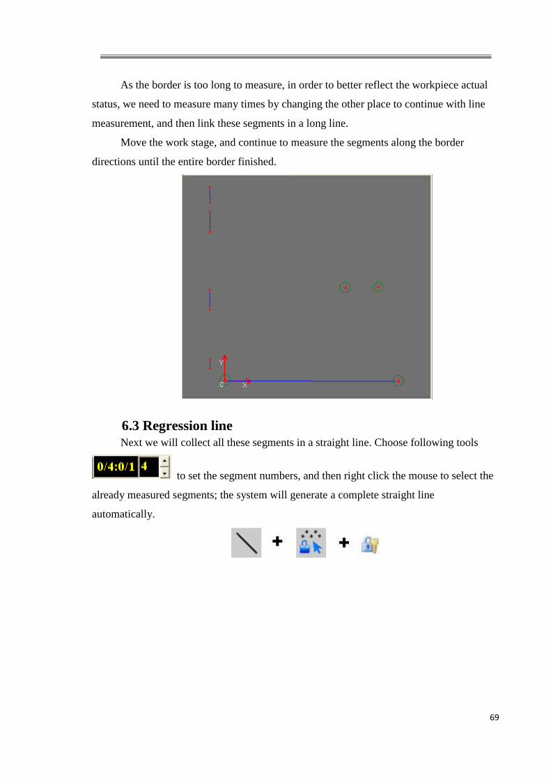
As the border is too long to measure, in order to better reflect the workpiece actual

status, we need to measure many times by changing the other place to continue with line

measurement, and then link these segments in a long line.

Move the work stage, and continue to measure the segments along the border

directions until the entire border finished.

6.3 Regression line

Next we will collect all these segments in a straight line. Choose following tools

to set the segment numbers, and then right click the mouse to select the

already measured segments; the system will generate a complete straight line

automatically.

70

In the same way, measure the line on the opposite side. Next, select “Distance

measure” and “Line measure” in the compound tools, and then right click the mouse to

select the two circles in geometric window. The system will automatically calculate the

two lines distance, the data shows as follows.

71

The same method can also be applied for measuring the bigger circle, please refer to

chapter “3.9 Compound measuring function”.

6.4 SPC Control

All elements measurements have been completed, next we will carry out SPC

control for the already measured elements. Click the mouse to select an element in the

object list, and then double click on the attribute column of the controlled element, e.g.

take diameter of circle as the controlled element, just double click on the diameter column,

and the system will prompt popup a dialog box.

72

The controlled items can be modified according to your requests. Fill out the

standard values and tolerance, mark a “√” before SPC, then the control complete for the

measuring elements. The already controlled elements can be recognized by turning blue in

front.

Other elements can also be controlled in the same way.

Until now, we have completed all measuring tasks according to the measuring

requirements. For the full automatic system, the greatest strength is carrying out inspection

in full automatic ways. Before taking measurement, you should tell the machine how to

measure, what be measured. All we do as above is to tell the machine where it need to

inspect, what should be inspected, and record them in turns in the object list. These

procedures will help the machine to do full automatic inspection efficiently.

73

The machine itself does not know how to measure, only after we tell the machine

how to do, can the machine learn by itself later according to your ideas, so we called this as

“Learning function”. We will take much easier later when the machine learn by itself.

We will save the learning procedures after complete edit the program and put away

for future use. Click” Save project” in the “File” menu. And open project in the same

format.

Next, the program can be running by itself, the details please refer to Chapter”3.5

Object list and learning function area”.

6.5 Workpiece datum setting

Workpiece datum setting is measure standard of workpiece, and this standard will

avoid problem of workpiece different positions placed every time.

It is just find position standard before inspection, and following step will finished by

machine automatically.

74

Right click in object list, then it show right-click menu, choose last item “Workpiece

datum setting”, open “Workpiece datum setting” window.

75

Six location methods are including: fixture location, crosshair location, object circle

location, point-set location, point-set circle-point-set line location, point-set line location.

6.5.1 Fixture location Design fixture according to measured product specs, then install the fixture on

machine workstage. Workpiece is fixed to fixture, so the relative location of workpiece and

machine is not change. This method is commonly used, system default is “Fixture

location”.

Click “Fixture location”, then press “Enter”, fixture location is set.

6.5.2 Crosshair location Using crosshair location not changing specification of “Image window”, make

crosshair location as workpiece location.

Press “shift” and drag crosshair by left key, make alignment of crosshair and

workpiece borders, then right click to bound up system hint, press “Enter”, datum setting is

finished.

76

When running learning steps, system bound up hints as follows, press “Enter” to

start running learning step.

This method demand worpiece placed location is parallel to crosshair. Cause it is not

easy operation, so not commonly used.

6.5.3 Object circle location Considering the round hole feature of the workpiece, this will need take the round

hole as the reference hole, and establish a coordinate system by the two round holes to

complete location for the workpiece, operations as follows.

Object circle location means that we take measurement for the two reference holes

by “object circle” measuring tools.

After selecting “objects circle location”, choose the check box for “set the workpiece

reference plane”, click “OK” to continue.

Find the first reference hole, then right click the mouse, and take the point as the

origin. Continue to find the second reference hole, and right click the mouse, the point will

determine the X axis directions. The inspection window follows.

The kind of location ways is very easy to operate, and with high location accuracy,

so it is widely used.

77

6.5.4 Point groups of circle location Make use of the round hole on the workpiece, and take the hole as the reference hole.

Establish a coordinate system by the two holes to complete location for the workpiece,

operations as follows.

“Point groups of circle location” means that we take measurement for the two

reference holes by same kind of measuring tools.

After selecting “Point groups of circle location”, choose the check box for “set the

workpiece reference plane”, click “OK” to continue.

Find the first reference hole, and then right click the mouse to take three points and

generate a circle, and take the point as the origin. Continue to find the second reference

hole in the same way; the point will determine the X axis directions. The inspection

window follows.

6.5.5 Point group of circle, point group of line location Make use of the round hole and line on the workpiece, and take the hole as the

reference hole; the line as the reference edge, establish a coordinate system by the two

elements to complete location for the workpiece, operations as follows.

“Point group of circle, point group of line location” means that we take

measurement for the reference holes by “Point groups of circle” measuring tools. And take

measure for the other reference line by “point group of line” measuring tools.

After selecting “Point group of circle, point group of line location”, choose the

check box for “set the workpiece reference plane”, click “OK” to continue.

78

Find the first reference hole, and then right click the mouse to take three points and

generate a circle, and take the point as the origin. Continue to find the reference line by

click taking at least two points to generate a line; the point will determine the X axis

directions. The inspection window follows.

6.5.6 Point groups of line location Make use of the line feature on the workpiece, and take the line as the reference

edge. Establish a coordinate system by the two lines to complete location for the workpiece,

operations as follows.

“Point groups of line location” means we take a reference line by same kind of

measuring tools.

After selecting “Point groups of line location”, choose the check box for “set the

workpiece reference plane”, click “OK” to continue.

Find the first reference line, and then click the mouse to take at least two points and

right click the mouse to generate a line, and take the line direction as the X axis. Continue

to find the second reference line in the same way; intersection point of the two lines is the

origin. The inspection window follows.

80

7. Checking

7.1 Quick Access

1. Click to start learning (the following steps will be recorded).

2. Select a learning model.

3. Define a mechanical datum plane. If you choose to use clamping, that means you

do not define the mechanical datum plane.

4. Measuring the object.

5. Double click the project you want to control in the “Object List” to load SPC.

6. Press will delete a checking step.

7. Click will exit the learning.

8. Click to move the platform to the position of the indicator, then click in the

Image window, OVM will automatically load data till finishing all the learning

steps.

9. Click , the platform will start the checking in loop until you click to stop.

81

10. Press the "Path" button to select an existing filename that SPC has exported. If

you have ticked "add to file", then the statistical data by SPC will be added to the

final part of the original file. If "add to file" is not selected, the software will

empty the previous data and then add the new data in; if you want to create a new

file, you simply need to name (use English letter) it after choosing the path. Press

“clear” will clear the path. Ps: The format exported by SPC can only be opened

by Q-PLUS.

7.1.1 Level Shift Copy and Rotate Copy

Level Shift Copy: to copy the selected object (can be more than one) along the

horizontal line.

Level Shift Copy is only usable under learning model.

For Example:

Input two circles on (0,0) and (3,0), like below:

In the Checking box, you will see the following picture. Click “geometrically or

manually input circle”, and press .

82

Set the value like the picture below and press “confirm”.

In Geometric window you will see the following picture, which tells that the

movement in Y direction is 3 and the copy number is 5.

83

Rotate Copy

Rotate copy the selected object (can select more than one).

Rotate Copy function is usable only under learning model.

For instance:

Input two circles on (0,0) and (3,0), like below:

84

In the Checking box, you will see the following picture. Click “geometrically or

manually input circle”, and press

Set the value like the picture below and press “confirm”.

In Geometric window you will see the following picture, which tells that the rotated

angle is 60º and the copy number is 5.

7.1.2 Explanation on the Detailed Procedure

85

Suppose that the object that you are to measure is a slice of circuit board, please

operate according to the following steps.

1. Fix the first circuit board (as reference to the following measuring

position) to the platform (use a clamping apparatus to fix so as to prevent the

circuit board from slipping. You can use clay to help fixing too).

Define the datum plane

86

If you use cross line to locate, the second and subsequent circuit

board should always be vertical or horizontal to the first circuit board.

○ vertical or horizontal shift

○ vertical or horizontal shift

87

○ rotate

Do not reverse the first circuit board (the front and back side might not be the same)

x reverse

x reverse

88

2. With the first circuit board, what we should do first is to define the

datum plane, but what’s the role of defining the datum plane? Because as we

have no clamping apparatus at hand, the position of each circuit board on the

platform can be the same, so we must tell the computer: Which position is

the standard position so that to avoid wrong judgments of the program which

are caused when rotating the circuit board.

3. Without clamping apparatus, we have the following five means to

define the datum plane: cross line positioning, object circle positioning, Point

Group circle positioning, Point Group circle and Point Group line positioning,

Point Group line positioning.

4. Presses Shift key, use the left mouse key to drag the Red Cross line

and let it aim at the right angle edge, and then right click to finish defining

the datum plane.

○ aiming at the right angle edge

89

x not aiming at the right angle edge

5. Find the circle to the left first, the right click to define the first datum

point; then find a circle to the right, right click to define the second datum

point. The line connects the first datum point and the second datum is the

X-axis we defined.

Picture of the first circuit board.

Right click at hole B to define the first datum point.

Right click at hole C to define the second datum point

90

The line connects the first datum point and the second datum point

(Line BC) is the X-axis we defined.

6. In the same way, we can find hole B and right click to define the first

datum point; and then find Hole A, right click to define the second datum

point. The line connects the first datum point and the second datum point

(Line BA) is the Y-axis we defined.

7. After defining the datum plane, start learning from the hole to be

measured in the first circuit board. Click will exit learning.

8. Take the first circuit board away from the platform and put the

second circuit board on the platform.

9. After manual learning, click or to find the datum point on the

second circuit board (use the same cross line or hole as the first circuit board).

Then you will see direction mark like to

91

help you move the platform. Stop moving when the red circle turn into green

and twinkling state. OVM will automatically measure the object.

10. After inputting the datum point (line), you can move the

platform to the correct position according to the data of the indicator, click

the image window again, OVM will load the data automatically till finishing

all learning steps.

11. Press to exit checking.

7.2 SPC

7.2.1 Step

1. Input the data that you want to analyze into SPC. You must enter Learning model

before you can use SPC.

2. The data that measures will have different attributes. Double click on that attribute

will list it in SPC controlling.

3. Enter a name for control item. For example: radius or R1. Input desired value in

standard value box, positive and negative tolerance box.

4. Stop the learning model by clicking . Click or will measure again the

previously learned objects till the end.

5. Press F4 to see results in SPC window.

7.2.2 Function Key of SPC

Create SPC Project: to clear all SPC data and create a new SPC project.

Open SPC Project: to open an existing SPC project.

Save SPC Project: save the current SPC project

Export To Excel: export the current SPC data to Excel.

Export To Word: export the current SPC project to Word.

Delete last group of data (including 2 to 6 sets of data)

Delete the last set of data

X-R Chart：Switch to Mean and Range Control chart.

Xm-R Chart：Switch to Median and Range Control chart.

X-Rm Chart：Switch to Specific Value and Mobile Range Control chart.

92

X-S Chart：Switch to Mean and Tolerance Control chart.

Three functions are available when right clicking on the control chart:

Full View：To show the graph with best size.

3D View： To draw the graph in 3D effect.

2D View： To draw the graph in 2D effect. (The default setting)

2D View

3D View

93

7.2.3 Data Analysis

Data form is divided into 3 parts in Data Analysis window: the upper part lists the

Data Analysis and some commonly used process norms, such as Ca, Cp and CpK. The

middle part lists the accuracy, precision of process, and process ability index. The lower

part lists the order number, item, standard value, and number of data, unqualified number

and its ratio.

94

7.3Graph Data

7.3.1 Mean and Range Control chart (X-R)

If the quality data can be reasonably grouped, use X control chart to analyze the

process and use R control chart to process variation

7.3.2 Median and Range Control chart (Xm-R)

Similar to X-R Control chart, but X control chart checking efficiency is lower while

the computation is simpler.

7.3.3 Specific Value and Mobile Range Control chart (X-Rm)

1. If the quality data cannot be reasonably grouped, use X-Rm control chart under the

following situations:

Only one data (such as manufacture efficiency and consuming rate) can be collected

at one time.

95

When the Process quality is very even so that no need to sample many times, such as

liquid density

When it is time-consuming and involves high cost to get the measuring value, such

as complicated chemical analysis and destructive inspection

2. If the quality data can be reasonably grouped, use X-R control chart to enhance

checking efficiency.

7.3.4 Mean and Range Control chart (X-S)

Similar to X-R Control chart, but the S Control chart is more efficient than R

Control chart in term of its checking ability while the computation is more complicated.

Use R Control chart if the sample number is less 10, otherwise use S Control chart.

96

7.3.5 Data Form

Data Form falls into two parts: the upper part shows the result of each set of

measuring (each row 2-6 samples) with their mean and range. The lower part displays the

order number of control data, the control item, standard value, and number of data,

unqualified number and its ratio.

7.4 Focusing

In Focusing window, select Enable Focusing, you will see a yellow box on the image

window. Move the platform then to place the edges within the box.

97

Click , the platform will automatically do the focusing.

You can use the default setting to do the focusing if you are under a low enlargement.

Otherwise, you should mark “accurate” and use the biggest value (drag the bar to the right)

under “sensitivity” before auto-focusing.

7.4.1 Focusing Indicator

Select “start”, you will see a yellow box on the image window. Move the platform to

place the edges within the box. Move the Z-axis, you will get a graph in the focusing

indicator window. If this graph is very disorderly, then you may need to click reset and

move the Z axis to get a graph until it looks normal. Next, you move the Z-axis in the

opposite direction and aim the green vertical line at the blue little cross line (the peak of

the wave). By doing this, you will get a clear focus.

mmuummaa pprroo - scienscope · company or services department to change the manual. in order to...

Documents