MNCs, Rents and Corruption: Evidence from China∗

Boliang Zhu †

Paper for Presentation at Princeton IR Faculty Colloquium

February 17, 2014

∗I am grateful to Yuen Yuen Ang, Lucy Goodhart, Isabela Mares, Yotam Margalit, Erica Owen, Laura Paler, SonalPandya, Pablo Pinto, Cyrus Samii, Yumin Sheng, Yusung Su, Matt Winters, and conference and seminar participants fortheir helpful comments and suggestions. I also thank Yumin Sheng for generously sharing his data. Yaman Cheng, XinjingLiu, Chen Wei and Qian Yang provided research assistance.†Assistant Professor, Department of Political Science, Penn State University, bxz14@psu.edu; NCGG Fellow,

Princeton University, bzhu@princeton.edu.

Abstract

How do multinational corporations (MNCs) affect corruption in developing countries? The ex-isting literature tends to assert that economic integration helps reduce corruption as integrationincreases market competition and efficiency, reduces rents, and promotes the diffusion of goodgovernance. Nonetheless, MNCs have been found to be active players in corruption in developingcountries. In this paper, I examine the consequences of MNC activities on corruption by conduct-ing a case study on China. I argue that MNC activities may facilitate rent-seeking behavior bycreating a market structure that contributes to higher rents and therefore make worse corruption inoperating countries. To test this argument, I leverage the within-country subnational variation anddraw from original data of objective corruption cases to construct measures of corruption. I findthat provinces with more MNC activities have a significantly higher level of corruption. The resultsare robust and consistent when possible endogeneity, law enforcement, and alternative measuresof corruption are considered. This finding has important implications for global anticorruptioncampaigns.

1 Introduction

How do multinational corporations (MNCs) affect corruption in host countries? Given the significant

role that MNCs are playing in the world economy and the substantial attention that both scholars and

international organizations such as the World Bank and the United Nations have given to quality of

governance, it is of great importance to understand the connections between MNCs and corruption.

The general account in the literature is that deepening economic integration tends to lower the level

of corruption because integration increases market competition and efficiency, reduces rents, and pro-

motes the diffusion of good governance.

Nonetheless, cross-border economic activities are not immune from corruption. Corruption scan-

dals involving foreign firms in developing countries have frequently made headlines. For instance,

Wal-Mart has recently been accused of paying bribes in Mexico and other emerging economies such

as Brazil, China and India to expand business. An investigation by the New York Times found, “Wal-

Mart de Mexico was an aggressive and creative corrupter, offering large payoffs to get what the law

otherwise prohibited. It used bribes to subvert democratic governance – public votes, open debates,

transparent procedures” (New York Times, December 17, 2012). In 2006, the Transparency Interna-

tional (TI) surveyed 11,232 business executives in 125 countries, asking them about their experience

with the business practices of firms from 30 leading exporting countries in their countries. The report

shows that foreign firms from giant exporting countries have a considerable propensity to pay bribes

in operating countries, especially in low income countries.1

These anecdotal evidences lead us to rethink the relationship between foreign investment and cor-

ruption. It seems that the existing literature has overlooked the strategic interactions between foreign

firms and host governments. Foreign direct investment (FDI) untaken by MNCs is different from

other forms of capital flows, such as remittances and portfolio investment, in the sense that it involves

the transfers of physical assets, human resources and technology, while demanding deep engagement

and long-term commitment from parent companies. In this regard, MNCs – the vehicles for FDI

– are sensitive to the political and economic conditions in host countries. Footloose foreign capital

1Transparency International. 2006. Bribe Payers Index Analysis Report. http://www.transparency.org/news_room/in_focus/2006/bpi_2006.

1

becomes illiquid ex post, under the risk of expropriation from opportunistic government and joint-

venture partner (Vernon 1971, 1980). These distinctive characteristics of FDI give MNCs incentives

and opportunities to exert potent influences on host countries. Existing studies have, for instance,

shown that MNC activities affect government spending and taxation (e.g., Garrett and Mitchell 2001),

income distribution (e.g., Jensen and Rosas 2007), labor rights (e.g., Mosley and Uno 2007), etc. Yet,

the research on the consequences of MNC activities on corruption lags behind.

Due to FDI’s ex post immobility and the risks of expropriation, MNCs employ various strategies

to protect and enhance their interests in host countries (e.g., Henisz 2000; Javorcik and Wei 2009;

Rodriguez et al. 2005). Likewise, when encountering corruption, MNCs are not passive victims but

active players. Empirical evidence based on firm surveys indicates that MNCs are as likely as their

domestic counterparts to engage in corruption (Hellman et al. 2000, 2002; Søreide 2006) and even

have a higher propensity to pay bribes in restricted sectors that offer higher rents (Gueorguiev et al.

2011). More importantly, entry of MNCs can change the market structure and competition in host

countries, which has important implications for corrupt activities.

This paper studies the relationship between MNC activities and corruption in developing countries.

It focuses on how MNC activities change the level of rents and thus rent-seeking behavior in host

countries. It argues that the presence of MNCs can be associated with a high level of corruption by

increasing rents in the market: First, while entry of MNCs helps exploit more market opportunities in

developing countries, it can create monopoly or oligopoly; Second, more productive MNCs can drive

local firms out of business and therefore reduce market competition. All these market imperfections

contribute to rents. When there exist higher rents, it not only reinforces firms’ ability of internalizing

the cost of corruption but also increases government officials’ incentives to engage in the quid-pro-quo

exchange of their control rights for bribes, consequently exacerbating corruption in the host country.

To test this argument, I conduct a case study on China, one of the largest FDI recipients and still

a relatively underdeveloped country. Testing the argument presents challenges of how to measure cor-

ruption in China. I rely on “objective” corruption cases reported by the procuratorate (jian cha yuan)

and collect an original dataset on the number of filed corruption cases, the amount of recovered cor-

rupt funds and the number of senior cadres disciplined (at or above the county or division level, xian

2

chu ji) for each province for each year from 1998 to 2007, to construct measures of corruption at the

provincial level. To deal with the fact that these measures are a mixed reflection of true corruption and

the efficacy of law, in the empirical analysis, I control for several variables that influence government’s

anti-corruption efforts and law enforcement. As robustness checks, I turn to survey data and use the

frequency of residents’ “witnessed” corruption that is arguably more objective and reliable, and the

level of perceived corruption as alternative measures. Finally I leverage a large firm survey conducted

by China’s National Bureau of Statistics and the World Bank and use firms’ expenditures on entertain-

ment and travel costs as a proxy for bribes. Empirical evidence shows that provinces with more MNC

activities tend to have a higher level of corruption. The results are robust and consistent after we take

into account possible endogeneity, law enforcement, and various political and economic variables. In

addition, I find that firms in provinces with more MNC activities in general pay more bribes.

The paper proceeds as follows. The next section reviews relevant literature. Then the paper devel-

ops an argument on how MNC activities can contribute to corruption in developing countries and then

presents a testable hypothesis within the context of China. Following that, the paper discusses the re-

search design and measurement of corruption. After that, systematic empirical analyses are conducted

to examine the determinants of corruption in China. Finally, it concludes.

2 Literature Review

Corruption is generally defined as the “misuse of public office for private gain” (Bardhan 1997; Rose-

Ackerman 1999). The publication of the Corruption Perceptions Index (CPI) by the TI has greatly

contributed to the empirical research of corruption. Existing empirical studies have, for instance,

shown that corruption undermines public goods provision, impairs domestic investment and retards

economic growth (see, e.g., Fisman and Svensson 2007; Mauro 1995). In addition, a growing body

of literature suggests that corruption reduces inflows of foreign investment. Not only does bribery

increases the costs of doing business, but the secrecy of corruption also adds uncertainty and risks (e.g.,

Wei 2000; Wei and Shleifer 2000). Yet, the research on the consequences of economic integration in

general, inward FDI and MNCs in particular, on corruption lags behind. The existing literature tends to

3

assert that deepening economic integration lowers the level of corruption because integration increases

market competition and efficiency, reduces rents, and promotes the diffusion of good governance. The

causal mechanisms typically suggested in the literature can be put into one of two broad categories:

competition and diffusion.2

The competition argument hypothesizes that increasing competition from foreign products and

firms reduces the rents enjoyed by firms, thus decreasing the incentives for corruption (Ades and

Di Tella 1999; Sandholtz and Gray 2003, 765-6; Treisman 2007, 236). International competition

drives down firms’ profits. If bribes are extra taxes on firms, in the case of low marginal gains due

to fierce competition, then corruption means higher business costs that can drive firms out of the

market. Moreover, in a globalized world with high capital mobility, corrupt officials’ ability to extract

rents may be largely restricted because capital can simply choose to leave and look for alternative

investment locations. According to this argument, competition associated with economic integration

tends to decrease corruption.

Economic integration can also affect corruption through diffusion. Scholars argue that “[t]he in-

teractions associated with trade and cross-border investment may also be mechanisms for the com-

munication of ideas, values, and norms” (Sandholtz and Gray 2003, 767). Since advanced Western

countries dominate both international trade and foreign investment, norms and values such as demo-

cratic governance, rule of law, property rights protection, etc. will be promoted globally through

cross-border economic activities. Thus, the expectation is that the more deeply a country integrates

into the global economy, the higher the likelihood that it will adopt these norms and values and will

therefore be less corrupt. Moreover, neoliberal policies are found to be associated with a lower level

of political corruption (Gerring and Thacker 2005). If globalization helps diffuse these policies, we

should expect countries that are more integrated into the world economy to be associated with less

corruption.

All of the above explanations are sensible. Nonetheless, the strategic interactions between for-

2In addition to these two arguments, scholars suggest that MNCs often have high corporate responsibilities and well-established internal corporate codes, and face regulatory pressures and legal constraints from both home countries andinternational anti-bribery conventions, all of which deter MNCs from engaging in corruption in host countries. See, e.g.,Rose-Ackerman (2002).

4

eign firms and host countries are much more complex than what has been suggested in the literature.

Evidence based on firm surveys indicates that MNCs are as likely as their domestic counterparts to

engage in corruption (Hellman et al. 2000, 2002; Søreide 2006) and have a considerable propensity

to pay bribes in operating countries, especially in low income countries (Transparency International

2006). That MNCs adopt different entry modes in host countries with differing levels of political and

contractual risks has been widely documented (e.g., Henisz 2000; Javorcik and Wei 2009; Rodriguez

et al. 2005). Likewise, MNCs are likely to adjust their investment and business strategies according

to local corruption environments in host countries. As Hellman et al. (2000, 7) noted, MNC activities

can be “directed into illicit channels with highly detrimental social and economic consequences.”

Recently, scholars have devoted attention to the detrimental consequences of MNCs on corruption.

For instance, Robertson and Watson (2004) find that a rapid rate of increase or decrease in FDI leads

to a high level of perceived corruption. Pinto and Zhu (2008) find that FDI inflows are likely to in-

crease the level of corruption in less developed non-democracies while reduce corruption in advanced

democracies. Leveraging a list survey experiment in Vietnam, Gueorguiev et al. (2011) provide evi-

dence that foreign firms are more prone than local firms to pay bribes in restricted sectors that yield

higher rents.

Empirically, the existing literature studying economic integration and corruption relies heavily on

the “subjective” measures of perceived corruption constructed by institutions such as the TI and the

World Bank, which are subjective to biases (see more discussions later). Moreover, as Knack and

Azfar (2003) point out, empirical work relying on perceived corruption suffers from sample section

bias because small countries are less likely to be covered by most available corruption perceptions

indices. Given these drawbacks in cross-national studies, a within-country research design may limit

the scope of generalization, but it helps deal with the sample selection bias and also allows us to

take advantage of multiple measures of corruption (both “objective” and “subjective”) for robustness

checks.

5

3 The Argument

The existing literature tends to assert that FDI inflows are likely to reduce corruption in host countries

through increasing competition and efficiency, reducing rents, and diffusing good governance, norms

and values. Yet, such a simple generalization overlooks the specific nature of MNCs and the strate-

gic interactions between MNCs and host governments. MNCs arise from taking advantage of their

ownership-specific advantages to overcome imperfections in arm’s length markets (Dunning 1988,

1992; Caves 1996). To be able to invest in foreign countries, a firm must possess some firm-specific

assets (ownership advantages) that are sufficient to overcome the disadvantages it faces when compet-

ing with indigenous firms in the host country. These proprietary assets include, for instance, advanced

technology, brand names, product differentiation, managerial and advertising skills, and access to

international market, which are of a public-goods character. In this sense, entry of MNCs implies

more than a simple import of foreign capital. In order to protect and enhance their proprietary assets,

MNCs actively adjust their entry mode and investment strategy to local environments in host coun-

tries (Henisz 2000; Rodriguez et al. 2005). The kind of entry mode and investment strategy adopted

by MNCs has important implications for understanding the consequences of MNC activities in host

countries. As Blomstrom and Kokko put, “[f]irms investing abroad therefore represent a distinctive

kind of enterprise and the distinctive characteristics are pivotal when analyzing the impact of foreign

direct investment on host countries” (1997, 2).

It has been well-established that corruption deters foreign investors as corruption and its inherent

secrecy and uncertainty add extra costs of doing business (Javorcik and Wei 2009; Wei 2000; Wei and

Shleifer 2000). Yet, not all foreign investors are deterred by corruption and a considerable number of

them have been found to actively engage in this quid-quo-pro business (Hellman et al. 2002, 2003;

Søreide 2006). When analyzing the effect of MNC operations on corruption in host countries, we

need to explore how the “distinctive characteristics” of MNCs determine their market strategies in

different host countries and the consequences of these market strategies on corrupt activities. Since

MNCs compete with very different groups of indigenous firms in developing and developed countries,

this paper focuses on the consequences of MNC activities in the former where local firms tend to be

6

relatively small, weak and technologically backward.

The political economy of corruption literature has convincingly shown that rents accruing from

natural resources exploitation or a lack of competition in the economy foster corruption (Ades and

Di Tella 1999; Rose-Ackerman 1999). In this sense, MNCs can affect corrupt activities in operating

countries by altering the market structure and the degree of competition and therefore the amount of

rents.

MNCs that pursue monopolistic or oligopolistic market positions can contribute to higher rents by

entering into new markets with high entry barriers in host countries. In developing countries, many

market opportunities remain under- or un-exploited, especially in industries with high entry barriers

exercised by scale economies, technology and capital requirements, product differentiation, and so

on. Yet, it is exactly the existence of these entry barriers that give rise to MNCs (Caves 1996). The

proprietary assets possessed by MNCs enable them to enter into these new markets whose barriers are

too high for indigenous firms. Therefore, MNCs are more capable than local firms of exploiting market

opportunities in the host country. Firms in these new markets often enjoy higher rents as competition

is limited because of high entry barriers.

Furthermore, the public-goods nature and scale economies inherent in the proprietary assets often

drive MNCs to pursue monopolistic or oligopolistic market positions (Blomstrom 1986; Lall 1979; Li

and Resnick 2003, 182; Stopford and Strange 1991). MNCs, large ones in particular, possess various

monopolistic advantages such as advanced technology, easy access to capital, and specialization in

capital- and skill-intensive activities, and thereby have enormous market power and have shaped the

world economy in a significant way. After entering into new markets in the host country, MNCs

may create and thereafter enhance the entry barriers for local firms by introducing new technology

and differentiated products and raising capital intensity of production. Moreover, MNCs may collude

with or lobby host governments to shelter them from foreign counterparts’ competition (Dunning

1992). Thus, entry of MNCs into these new markets may result in monopolistic or oligopolistic market

structures and imperfect competitions. Firms in such markets enjoy higher rents than what could be

earned in perfect competitive ones.

MNCs can also lead to rent creation by crowding out domestic investment and decreasing com-

7

petition in host countries. Foreign firms represent advanced technology, sophisticated managerial and

marketing skills, easy access to capital and international market, etc. On the contrary, indigenous firms

in developing countries are typically small, weak and technologically backward. When more compet-

itive and productive foreign firms enter the market, they can drive some local firms out of business,

therefore decreasing the level of competition in the economy. A counter argument is that entry of

MNCs generates positive spillover effects through forward or backward linkages and increases mar-

ket competition. Nevertheless, an overwhelming majority of empirical evidence has suggested that

spillover effects are conditional on the characteristics of host countries. Positive spillover effects take

place only when host countries achieve a certain level of development and absorptive and technologi-

cal capacity (e.g., Blomstrom et al. 2001; Blomstrom and Kokko 1997; Blomstrom et al. 1994; Kokko

1994). Many empirical studies have shown that FDI inflows and the presence of MNCs increase mar-

ket concentration and result in imperfect competition in developing countries (e.g., Blomstrom 1986;

Blomstrom and Kokko 1997; Lall 1979; Newfarmer 1979). When market is concentrated and compe-

tition is decreased, firms, more competitive and productive MNCs in particular, tend to enjoy higher

rents.

So far, we have discussed that MNC activities in developing countries may contribute to rent

generation: MNCs can create monopoly or oligopoly in new markets whose entry barriers are too high

for local firms; entry of more competitive and productive foreign firms can drive domestic firms out of

the market and leads to imperfect market competition. When firms enjoy higher rents, it makes them

more able to internalize the cost of bribes. To the bureaucrats in the host country who have influence

over these firms, it increases the value of their control rights; consequently, they have more incentives

to engage in the quid-pro-quo exchange of their control rights for bribes (Ades and Di Tella 1999).

It should be noted that rents per se do not necessarily lead to corruption. Firms can seek rents either

through legal forms such as lobbying, in which favorable regulations are public goods for an entire

industry or market, or through illegal forms such as bribery, in which favorable policies are private

goods to those who have paid bribes. Existing research has shown that corruption and lobbying can be

substitutive strategies for firms to influence government regulations; bribing tends to be firms’ most

likely and cost-effective strategy in developing countries where firms’ capital level is relatively small

8

(Campos and Giovannoni 2007; Harstad and Svensson 2011).

Apparently, MNCs have the option to exit and are thus able to force host governments to reduce

corruption and improve governance. However, FDI is different from simple capital flows such as

portfolio investment and remittances in that it involves cross-border transfers of physical assets, human

recourses and technology, while demanding deep engagement and long-term commitment from parent

companies. Once investment takes places, a portion of the investment has sunk and the bargaining

power has started to shift to the host government (Vernon 1971, 1980). The bargaining power of MNCs

depends on the availability of alternative market opportunities and the cost of relocation compared to

the amount of bribes. On the part of MNCs, FDI represents an eagerness to take advantage of market

opportunities in the host country (Robertson and Watson 2004, 388). Bribery is likely to be a chosen

strategy. Therefore, I expect that more FDI and MNC activities are likely to increase corruption in

developing countries.

3.1 MNCs and Corruption in China

Since its reform and opening-up in 1978, China has become the largest FDI recipient in the develop-

ing world. Annual FDI inflows have grown from almost zero to more than $250 billion in 2012. It

is widely believed that inward FDI has been one of the major engines of China’s economic miracle.

Nonetheless, the surge of FDI inflows has also generated some unintended consequences. In 2008, a

high-ranking official in the Ministry of Commerce (MOC) was arrested for corruption of approving

foreign investment. This case involved several high-ranking officials in government agencies in charge

of regulating FDI, including the MOC, State Administration for Industry and Commerce (SAIC) and

State Administration of Foreign Exchange. In and of itself, the case is not unique. In China, MNCs

have been known to bribe officials through a variety of ways including offering government officials

direct cash payments, occupational trainings, foreign trips, overseas education opportunities for offi-

cials’ children, and so on (South China Morning Post, October 8, 2007). Anecdotal evidence aside,

there is no systematic empirical study yet on how FDI inflows and MNC activities may affect corrup-

tion in China.

As discussed above, in developing countries FDI inflows and MNC activities may cause an increase

9

in corruption: entry of MNCs can contribute to rent creation by entering into new markets with high

entry barriers and pursuing monopolistic or oligopolistic positions and by driving local firms out of

the market and decreasing competition; higher rents enable firms to internalize the cost of corruption

and increase the value of bureaucrats’ control rights and thus their incentive to extract bribes. It

should be acknowledged that, in a large and diversified economy like China MNCs may cause rents

in some industries and regions while diminish them in others. Thus both the positive and negative

effect of MNC activities on corruption could be at play. The empirical question is then which effect

prevails.3 This study is intended to estimate the net effect of MNC activities on corruption in China. In

a licensing society such as China where all industrial and commercial enterprises require government

authorization to operate, corruption tends to pervasive (Manion 1996). When inward FDI and MNC

operations contribute to higher rents in the market, corrupt activities are likely to increase. Thus, I

hypothesize that more MNC activities lead to higher levels of corruption in China.

4 Research Design

To test the above hypothesis, I leverage the within-country subnational variation in China. There are a

few reasons for such a research design. First, cross-national studies of corruption have mainly relied

on perception-based measures constructed by institutions such as the TI, World Bank and PRS group.

The publication of these indices has significantly advanced empirical research of corruption and pro-

vided important insights into the causes and consequences of corruption. These “subjective” measures

have also received much criticism as experts’ opinions can be biased and residents in different coun-

tries may understand corruption quite differently (see more discussions later). Second, as Knack and

Azfar (2003) point out, existing studies on economic integration and corruption suffer from sample

selection bias, because small countries are less likely to be covered by most available corruption per-

ceptions indices and they tend to be more open naturally given their small domestic markets. When

including more small countries in their sample, they find that trade openness does not affect corruption

significantly. This finding suggests that the empirical evidence on the relationship between economic

3An alternative empirical strategy is to estimate the effect of MNCs on corruption in different industries. However, theavailable industrial FDI data is not disaggregated enough to allow such a study.

10

integration and corruption from cross-national analyses can be dependent on the sample size in the

regressions. Third, by focusing on a single country, I am able to take advantage of multiple measures

of corruption, both “objective” and “subjective,” thus mitigating the concerns of measurement prob-

lems in the cross-national analyses. Finally, China, the largest FDI recipient in the developing world

and still a relatively underdeveloped country, provides an ideal case to study the relationship between

MNC activities and corruption. During the reform and openness era when China’s economy has been

increasingly decentralized, provincial governments have obtained substantial policy autonomy, which

has resulted in market fragmentation and local protectionism. Despite its authoritarian regime, China

is by far one of the most decentralized countries in the world (Landry 2008). Montinola et al. (1995)

argue that China is a de facto federal system. All of these justify the focus of subnational variation and

the use of provinces as units of analysis.

4.1 Measuring Corruption at the Provincial Level

The biggest challenge is how to measure corruption within China. Two measures of corruption – “sub-

jective” and “objective” – are commonly used in empirical studies. Subjective measures of corruption

are indices of perceived corruption. These indices are aggregated from different surveys of inter-

national and local businessmen as well as country experts and residents. Objective measures use the

actual number of corrupt convictions as a proxy for corruption. The quality and reliability of both mea-

sures are questionable.4 Subjective indices are measures of opinions of corruption which are largely

influenced by respondents’ cultural backgrounds, identification, and social norms.5 The opinions of

international businessmen and country experts are also biased because the majority of them come from

advanced Western countries. The problem of objective measures is that they are a mixed reflection of

true corruption and the efficacy of law enforcement. Recently, scholars have turned to another “objec-

tive” measure that surveys people or firms’ experienced corruption, such as the TI’s Global Corruption

Barometer and the World Bank Business Environment Survey. The experienced corruption is arguably

4See, e.g., Glaeser and Saks (2006) and Treisman (2007) for discussions of available sources of corruption measuresand their problems.

5This problem is mitigated in a within-country setting as respondents are more likely to have a common understandingof corruption.

11

a more reliable measure because it is based on respondents or firms’ own experience.

To deal with these problems in measuring corruption, I adopt several strategies to check the ro-

bustness of the findings. First, I rely on objective corruption cases as a proxy.6 The measures based on

corruption cases give us advantages to capture different aspects of corruption, including the level of

bribes in each corruption case, the per capita corruption burden, and the frequency of high-ranking of-

ficials involved in corruption, all of which are critical to understand the consequences of cross-border

economic activities. To deal with the fact that objective corruption cases are a mixed reflection of

true corruption levels and law enforcement, I explicitly control for law enforcement in the regression.

Second, I turn to individual survey data and use both “perceived” and “witnessed” corruption as alter-

native measures. The latter is based on respondents’ personal experience. This variable is arguably a

more objective and reliable measure of the prevalence of corruption and is unlikely to be affected by

law enforcement. Finally, I utilize firms’ expenditures on entertainment and travel costs as a proxy for

bribes and examine whether firms in general pay more bribes in provinces with more inward FDI and

MNC activities.

4.1.1 The Procuratorate and Corruption Investigation

The procuratorate (jian cha yuan), part of the government’s judicial system, is responsible for the in-

vestigation and prosecution of corruption cases. Corruption is defined as the misuse of public office

for private gain. However, in China corruption is defined more broadly. It is “virtually any form of

‘improper’ behaviour by either a state official or a member of the Communist Party” (Wedeman 2004,

896-7).7 Since 1997,8 corrupt cases reported have included graft, bribery, and misappropriation of

public property, as well as violations of civil rights and official malfeasance by state employees. Ap-

parently graft, bribery and misappropriation of public property are in accordance with the conventional

definition of corruption. Ideally, the cases of the first three categories should be used as a measure of

corruption. However, available data is not detailed enough to allow us to disaggregate corruption cases

6This approach has been widely used in the studies of corruption in the U.S. (e.g., Glaeser and Saks 2006; Meier andHolbrook 1992), and recently in the research of corruption in China (Guo 2008; Manion 2004; Wedeman 2004, 2005)

7For a discussion of the definition of corruption in China, see Wedeman (2004, 896-9).8In 1997, China modified its criminal procedure law and the new law excluded copyright theft and fraud, tax evasion

and resistance, and illegal imprisonment by non-state employees from corruption.

12

for each province. Fortunately, according to the data at the national level, the first three types of cor-

ruption account for an average of 82% of total corrupt cases filed from 1998 to 2007. Thus, even if

corruption is narrowly defined, the filed corrupt cases can still be a good proxy.

To understand how corruption cases are investigated, it is important to elucidate the legal proce-

dure. The procuratorate is responsible for both investigating and prosecuting economic crimes and

criminal violations of discipline. It conducts an initial investigation to decide whether or not to accept

a case (shou’an) for formal investigation. Based on a complete investigation of the accepted cases,

the procuratorate files cases (li’an) with the People’s Court if there is adequate evidence of crime,

and it then serves as the prosecutor (Wedeman 2004, 910-11; see Du and Zhang 1990). The procu-

ratorate investigates corruption cases from several sources: cases disclosed or reported by the public,

cases referred by the supervisory bureaus that have the responsibility to monitor public officials and

maintain administrative discipline, and those turned in by the disciplinary inspection committees that

are responsible for investigating malfeasance of Party members.9 Therefore, politicians’ willingness

and political considerations as well as the public’s awareness of corruption can all affect the inves-

tigation of corruption cases. The information revealed includes the total number of filed corruption

cases, senior cadres disciplined (at or above the county and division level, xian chu ji), corrupt cases

or persons involving the Party, administrative, judicial, and the economic supervision systems, total

corrupt funds recovered, and so on. Not all data are available for each province for each year. The

most comprehensive and consistent data are the total number of filed corruption cases, the amount of

corrupt funds recovered, and the number of senior cadres disciplined. I have thus collected the data on

these three categories by reading various annual procuratorial reports for each province for the period

of 1998 to 2007 to construct measures of corruption.

To understand what the data is measuring, it is important to clarify what the term “degree of cor-

ruption” means. Consider a simple example given by Lambsdorff, 4: “10 percent of all public servants

take a bribe of $200 each, 5 times a year in exchange for awarding a contract that results in a gain of

$500 each for corrupt private contractors.” In this case, the level of corruption can be understood as

9In practice, the supervisory bureau and the disciplinary inspection committee conduct joint investigations becausemost state officials are Party members. Due to a lack of judicial authority, both authorities are limited to investigatingnon-criminal violations of administrative discipline and Party law (Wedeman 2004, 905).

13

“the frequency of corrupt acts, the amount of bribes paid or the overall gain that contractors achieve via

corruption.” Since it is almost impossible to assess the overall gain that contractors obtained through

corruption, I focus on the frequency of corrupt activities and the amount of bribes. According to

Wedeman (2004, 2005), corruption in China has intensified in terms of the amounts of corrupt money

and “major cases,” but the total number of corruption cases has remained mostly unchanged since the

1989-90 anticorruption campaign. To capture the severity of corruption, I first utilize corrupt funds

recovered per filed case as a measure of corruption that explicitly addresses the level of bribes involved

in each case. Second, total recovered corrupt funds are used to capture overall bribes. This variable

is normalized by total population10 such that it gauges the per capita losses or burden of corruption.

Finally, the level of corruption can be high because more high-ranking officials are involved. I employ

senior cadres disciplined per 10,000 public employees to capture this dimension of corruption.

It should be noted that corruption takes time to detect and the whole process of investigation and

prosecution may last a few years. Guo (2008) finds that the average latency period of corruption cases,

referring to the time it takes to detect the corruption case since a public official commits a corrupt act

for the first time, increases from about 3 years in late 1990s to 5 years or even more in early 2000s.

In addition, the actual number of corruption cases investigated each year may depend on leaders’

political willingness and considerations. Thus, the annual number reported by the procuratorate at

the provincial level may not well reflect each year’s actual level of corruption in each province. The

temporal variation in the dataset could be misleading.11 To deal with this problem, I rely on cross-

sectional variation and take an average of these three corruption variables for two periods, 1998-2002

and 2003-2007.12 To maximize the number of observations, I average the variables for each province

that has at least one observation within each of the two 5-year spans. All three variables are logged in

order to deal with skewed distributions.

[Figures 1, 2 & 3 about here]

Figures 1, 2 and 3 respectively show the level of corruption across China based on the three mea-

10Empirical results are consistent if total recovered corrupt funds are normalized by GDP.11Simple OLS regressions with fixed effects based on panel data show that the results are consistent with those obtained

from cross-sectional regressions. Results are available upon request.12They are also consistent with government officials’ terms in China.

14

sures. We can see that provinces located in the coastal, middle and southwestern areas tend to have

higher levels of corruption than others. Tibet, in particular, stands out as a corrupt province in the

western region, especially in terms of corrupt funds recovered per filed case and per capita corruption

losses.13

The advantage of the data is that the reporting and classifying procedures are standard across

provinces and consistent over time. Moreover, the data allows us to explore different dimensions

of corruption. The major concern of these measures based on corruption cases is that they are a

mixed reflection of true corruption and the effectiveness of law enforcement. The gap between the

discovered and the true corruption levels is a function of the efficacy of law enforcement. To deal

with this problem, I construct several measures of local government’s anti-corruption efforts and law

enforcement. In addition, as robustness checks, I rely on residents’ “perceived” and “experienced”

corruption as well as firms’ entertainment and travel costs as a proxy for bribes.

4.2 Independent Variable

The independent variable, MNC activities, is measured by the percentages of inward FDI14 and trade

by foreign invested enterprises (FIEs) to GDP.15 In China more than 50% trade is conducted by FIEs

and a substantial part is actually intra-firm trade. In this sense, trade to a large extent reflects foreign

firms’ activities rather than market competition. In addition, trade may give rise to opportunities for

corruption that is related to customs clearance and distribution of import licenses and quotas (Knack

and Azfar 2003, 3). I thus conduct a principal component factor analysis of these two variables to

obtain a factor score as a measure of MNC activities.13Although it would be interesting to examine why Tibet is more corrupt than other provinces in the western region, it

is beyond the scope of this study.14The use of FDI inflows allows us to capture the corruption related to the regulations of foreign firms’ entry, which is a

serious issue in China (). FDI inflows are also a good proxy for FDI stocks given that the correlation between FDI inflowsand stocks is 0.94 for the period of this study. Empirical results are substantively the same if we use FDI stocks.

15FDI data comes from China Data Online and trade data from China Statistical Yearbook. Both variables are loggedto deal with skewed distributions.

15

4.3 Law Enforcement

Since the corruption measures based on filed cases are a mixed reflection of true corruption levels

and the efficacy of law, in order to estimate the effect of MNC activities on corruption, we need to

control for law enforcement in regressions. I use several measures to capture law enforcement and

local government’s anti-corruption campaigns. The first is a measure of “bureaucratic integration.”

Recently, scholars have suggested that China’s central government has resorted to control provincial

officials through its monopoly power of cadre appointment (Huang 1996; Sheng 2007). Huang and

Sheng’s studies found that the pro-center provincial leaders are more likely to implement policies

in accordance with central government, fighting harder against inflation and getting less favorable

fiscal treatment. “Bureaucratic integration gauges the propensity of provincial officials to comply with

central policy directives by virtue of their future career prospects or prior career trajectories” (Sheng

2007, 414). Since anticorruption has been one of the central government’s top priorities (Wedeman

2005), I expect that the more centrally-oriented provincial leaders are, the more vigorously they fight

against corruption.

I use the bureaucratic integration variable initially constructed by Huang and extended by Sheng as

one of the proxies for provincial leaders’ anticorruption efforts. According to political leaders’ posi-

tions in the party system and relevant work experience, they are placed into one of the four categories:

provincial leaders holding a concurrent position at the center are assigned a score of 4; those who

have at least three years of work experience at the ministerial or vice-ministerial level in the central

government are given a score of 3; provincial officials who have worked at least three years in other

provinces get a score of 2; and lastly, “localists” who are promoted within the province are scored

1 (Sheng 2007, 414-7). High scores represent more centrally-oriented leaders, who therefore are ex-

pected to devote more resources to fighting against corruption.16 I expect the bureaucratic integration

variable to be positively correlated with the dependent variables constructed from corruption cases,

given that the more resources government devotes to fighting against corruption, the more corruption

cases it detects.

The second measure is a dummy variable of the four municipalities directly administrated by the

16The original data is only available up to 2005. Data for 2006 and 2007 was updated by author.

16

central government. Given their unique positions in the administrative system, I expect that the central

government monitors these four municipalities more closely, and thus they fight harder against cor-

ruption and detect more corruption cases. The third one is a measure of the public’s trust in the court

system, which is constructed from the first two waves of Asian Barometer Surveys.17 In the survey,

one question asks how much trust respondents have in the courts. Respondents choose from 1 – a great

deal of trust, 2 – quite a lot of trust, 3 – not very much trust, and 4 – none at all. I first reverse the

order and then take the mean of all responses for each province as a measure of the effectiveness of the

court system. The public’s trust in the courts can be influenced by corruption cases reported. However,

corruption cases only account for a very small proportion of total cases accepted by the courts. For

instance, in 2008 they are less than 3% of total accepted criminal cases and are only 0.35% of total

accepted cases by the courts. In addition, the public’s trust in the courts is also dependent on people’s

personal experience. Thus this variable is likely to capture the overall efficacy of the court system.

I expect that the more trust the public has in the courts, the more effective the court system is and

therefore the more corruption cases it detects.

Alternatively, we could use the expenditure on public security agency, procuratorial agency, and the

court of justice as a proxy for local government’s anticorruption campaigns. However, this variable is

problematic for at least two chief reasons. First, it is extremely highly correlated with total government

expenditure that is commonly used to measure the size of government in the literature.18 Second, more

expenditures could result in more corruption rather than greater anti-corruption efforts.

4.4 Other Control Variables

Regarding the determinants of corruption in the literature, the most significant finding is that higher

GDP per capita – a proxy for economic development – is associated with lower corruption levels even

when possible endogeneity is considered (Treisman 2007). This finding has been confirmed by many

other studies in both cross-national and within-country analyses (see, e.g., Ades and Di Tella 1999;

17The two surveys were conducted in 2002 and 2008 respectively. Data from the first survey are used to construct themeasure of the effectiveness of the court system for the 1998-2002 period, and those from the second survey used for the2003-2007 period.

18The Pearson correlation of these two variables is 0.94 for the period of this study, which renders it impossible toidentify the underlying causal mechanism.

17

Glaeser and Saks 2006; Treisman 2007). Economic development not only leads to the rationalization

of economic and political systems, but it also contributes to the spread of education and literacy, all

of which should help reduce corruption. However, GDP per capita is likely to be endogenous to both

MNC activities and corruption. To deal with the endogeneity, I take advantage of a natural experiment

created by China’s reform and openness. Before the reform and openness, China had virtually no

foreign investment. Thus, I utilize the data from two periods before China’s reform and openness:

1969-1973 and 1974-1978 as proxies for GDP per capita in 1998-2002 and 2003-2007 respectively.

The GDP per capita before reform and openness not only helps mitigate the endogeneity problem,

but it also helps reduce the collinearity between GDP per capita and MNC activities. Moreover, it

is a good proxy for GDP per capita from 1998 to 2007. The Pearson correlation between these two

GDP per capita variables is 0.84. Additionally, I include total GDP to account for the effect of the

economy size, as the scale of an economy is an important determinant of the total amount of rents in

the market.19 The data of both variables come from China Statistical Yearbook.

Corruption may rise with the size of government, as bigger government means that officials have

more resources under their control, thereby more opportunities for bribery. Although empirical studies

provide mixed results on the relationship between government size and corruption (see, e.g., Gerring

and Thacker 2005; Montinola and Jackman 2002), to be consistent with previous studies, I control for

this variable in regressions. Government size is measured by the percentage of government expenditure

to GDP and the share of employees in state-owned units that include government agencies, Party

organs, social organizations, state-owned enterprises (SOEs), etc.20 Education is believed to help

reduce corruption because people’s political participation and civic engagement are positively related

to their education levels (see, e.g., Glaeser and Saks 2006). This variable is measured by the percentage

of population aged 6 or above who have at least some college education. Scholars also suggest that the

relatively high wages of public sectors to private sectors decrease the incentives for corruption (see,

e.g., Treisman 2000). When a public employee has a high paying position, s/he has less incentive

19Again, I use GDP before the reform and openness era as a proxy to deal with possible endogeneity problem. Resultsare consistent when both GDP per capita and GDP variables are lagged one period.

20Public employees in China are more broadly defined. For instance, managers and directors in SOEs and social organi-zations usually obtain the same status as government officials and sometimes are promoted into the government and Partysystems.

18

to jeopardize it by engaging in corruption. Thus we should expect that the higher relative wages

of public employees should be associated with less corruption. This variable is measured by the

ratio of average wages of state-owned units to private sectors. Scholars have also found that gender

impacts corruption (e.g., Swamy et al. 2001). Specifically, women tend to be more disciplined and less

tolerant of corruption. Therefore, a government with more female employees should be less corrupt.

However, the results on gender have been disputed recently (e.g., Sung 2003). I use the share of female

employees in state-owned units to capture the influence of gender. Finally, I include a dummy variable

for the second period to account for the effect of time trend given that corrupt funds tend to grow over

time.

The data used to measure education, government expenditure, size of public employees, and public

employees’ relative wages, all come from China Statistical Yearbook. Gender (the share of female

public employees) is measured based on the data from China Labor Statistical Yearbook. Government

expenditure is lagged a 5-year period to deal with possible endogeneity, and all other variables are

averaged as the same periods of the dependent variables. The descriptive statistics and the correlation

matrix of explanatory variables are shown in Tables D and E in Appendix.

4.5 Endogeneity and Selection Bias

Empirical studies suggest that higher levels of corruption reduce FDI inflows (e.g., Malesky and Sam-

phantharak 2008; Wei 1997, 2000). Thus, it is possible that corruption “selects out” certain types of

investors at the first place and leads to less inward FDI. Nonetheless, it should be noted that since

the paper argues that MNC activities contribute to corruption, if the endogeneity and selection at the

first stage were corrected, we would observe higher levels of MNC activities in more corrupt areas

and thus a larger effect of MNCs on corruption. In such cases, OLS regressions tend to underestimate

the positive effect of economic integration. Thus endogeneity is not a serious concern. To precisely

estimate the coefficient of MNC activities and to deal with the possible endogeneity and selection

biases, I take advantage of the spatial variation in China’s levels of economic integration and use

the geographic distance as an instrumental variable for MNC activities. Following Jensen and Rosas

(2007) and Larraın and Tavares (2004), I construct an instrumental variable for MNC activities at the

19

provincial level using the weighted geographic distance between China’s provincial capitals and the

five major economic centers21 around China. This instrumental variable is rooted in the gravity models

of international trade and FDI flows (see, e.g., Carr et al. 2001; Frankel and Romer 1999; Loungani

et al. 2002; Markusen 1995). Countries tend to trade more with their neighbors and FDI originated

from wealthier countries is more likely to flow into closer regions.22 I weigh the geographic distance

by these five economies’ real GDP per capita to capture the fact that more developed countries tend

to export more products and capitals. On average these five economies together account for approxi-

mately 59% of China’s FDI inflows and 42% of trade from 1998 to 2007. We have reasons to believe

that exogenous geographic distance and the five economies’ real GDP per capita are unlikely to have

a direct effect on China’s provincial corruption except through the channel of foreign investment and

trade.23 Sensitivity analysis is used to assess to what extent the empirical results are sensitive to the

potential violation of the exclusion restriction.24 The instrument variable is constructed as follows:

Zi,t =5∑

j=1

1

disti,j,t× GDP per capitaj,t (1)

where i = 1, 2, ..., N , j = 1, ..., 5, and t = 1, 2.

This instrumental variable measures the geographic closeness of China’s provinces to the five eco-

nomic centers. Thus, we expect that the closer a province is to these five cities, the more economically

21They are Hong Kong, Seoul, Singapore, Taipei, and Tokyo.22That geographic distance affects trade patterns is one of the most robust empirical regularities in the economic liter-

ature. With regard to FDI, the knowledge-capital model suggests that efficiency-seeking (vertical) FDI tends to decreasewith trade costs such as geographic distance, while market-seeking (horizontal) FDI increases with trade costs (Carr et al.2001; Markusen 1995). In China, before 1992, the Chinese government gave no access to market-oriented foreign firmsand thus all FDI was efficiency-seeking. Since 1992 when China started to open its market to foreign firms, efficiency-seeking FDI has still remained a considerable share. For market-seeking FDI in China, foreign firms also tend to locatein areas that are closer to their home countries, which give them advantages to import parts and components from parentfirms. For instance, Japanese and Koreans firms tend to concentrate in north China, such as Beijing, Liaoning, Shandongand Tianjian, while firms from Taiwan and Hong Kong operate mainly in southeastern China, such as Fujian, Guangdong,and Zhejiang. Thus, geographic distance is a good predictor of over MNC activities in China.

23Geographic distance impacts corruption through the activities that are related to distance. We have reason to believethat geographic distance has an effect on corruption primarily through the two major transnational economic activities –foreign investment and trade. However, it is possible that geographic closeness has an impact on corruption through labormovement, migration, or even the media. This kind of effects should be at margin because the cross-border movement oflabor and migration is still limited in China and the government highly restricts foreign media. In addition, Hong Kong,Japan, Korea, Singapore and Taiwan are all considered to be less corrupt than China. Thus we should expect a negativeeffect of geographic closeness on corruption through labor movement, migration, and foreign median. If this is the case,2SLS models tend to underestimate the positive coefficient of economic integration on corruption.

24Results are shown in Appendix.

20

integrated it is. Geographic distance is calculated using the ArcGIS 9.3 program. Real GDP per capita

data of the five economies between 1998 and 2007 are from Penn World Table.

5 Empirical Results

To examine the effect of MNC activities on corruption, I estimate the following two-stage least square

(2SLS) model:

MNCsi,t = δ + θ ∗GeoClosenessi,t +Xi,tπ + µi,t (2)

Corruptioni,t = α + β ∗MNCsi,t +Xi,tγ + εi,t (3)

Where i = 1, ..., N and t = 1, 2

Equation 2 and 3 represent the first and second stage regressions respectively. E[MNCs, εi,t] 6=

0 and E[GeoClosenessi,t, εi,t] = 0. To deal with possible heteroskedastic errors, the Generalized

Method of Moments (GMM) is used in 2SLS estimation.

5.1 The Effect of MNC Activities on Corruption

Given the small sample size, I start with some key determinants of corruption: MNC activities, GDP

per capita, GDP, government expenditure, size of public employees, and a time dummy. Model 1 in

Table 1 presents the OLS regression results. We can see here that the variable – MNC activities – is

positively and significantly correlated with corruption measured by corrupt funds recovered per filed

case.

To deal with possible endogeneity and selection bias, in Model 2, I fit a GMM 2SLS regression

model using weighted geographic closeness as the instrumental variable for MNC activities. In the

first stage regression (Model 2a in Table C in Appendix), the instrumental variable strongly predicts

provincial level of MNC activities and the F-statistic of the (excluded) instrument is 59.59,25 which

shows that the instrumental variable is valid and strong (see, Bound et al. 1995; Staiger and Stock

25All exogenous variables (included instruments) from the second stage regression are included in the first stage regres-sion. In the following 2SLS regressions, all F-statistics of (excluded) instruments in the first regressions are well above10. See Table C in Appendix for first stage regression results.

21

1997). After accounting for possible endogeneity and selection bias, the coefficient of MNC activ-

ities increases from 0.38 to 0.48, statistically significant at 1%. This confirms that OLS regression

underestimates the coefficient of MNC activities.

Given that the dependent variable is a mixed reflection of true corruption and the efficacy of law,

to estimate the direct effect of MNC activities on corruption, we need to control for law enforcement.

In Models 3, 4 and 5, I respectively add three variables – bureaucratic integration, a dummy variable

of the four municipalities directly administered by the central government, and the public’s trust in

the court system – as proxies for local government’s anticorruption efforts and law enforcement. We

can see that all three variables have expected regression signs and the coefficients of the first two

variables are statistically significant. The results suggest that centrally-oriented government officials

are more likely to comply with the central government’s anticorruption directives and thus detect

more corruption; the four municipalities fight harder against corruption; and the courts with more

public trust investigate more corruption cases. After we control for local government’s anticorruption

efforts and law enforcement, the variable – MNC activities – still has a positive effect on corruption

and its coefficient is statistically significant beyond conventional levels. Model 6 controls for the three

variables simultaneously. In Model 7, I add more controls – schooling, public employee’s relative

wages, and gender. Again, MNC activities positively and significantly affect corruption. Substantively,

take Model 7 for example, when all other variables are held constant, one standard deviation increase

of MNC activities will raise corrupt funds recovered per filed case by 0.48 units, which are about

U16,020 or $2,644 per filed case.26 These roughly equal to 64% of national average annual wage in

2007. The effect of MNC activities on corruption is both statistically and substantively significant.

The results in Table 1 also show that economic development (GDP per capita) significantly de-

creases corruption. In Model 7, all else being equal, one standard deviation change in GDP per capita

decreases the level of corruption by 0.63 units, approximately U18,848 or $3,110 per filed case. A

larger economy and a bigger government are both strongly associated with higher levels of corrup-

tion. One standard deviation increase in GDP, government expenditure and size of public employees

will result in more corruption by 0.23, 0.33 and 0.33 units respectively (roughly U12,551/$2,071,

26The U.S. dollar value is converted based on the exchange rate, 1$ = 6.06 Chinese Yuan.

22

U13,849/$2,285 and U15,851/$2,286 per filed case), when all other variables are constant.

[Tables 1 about here]

We have shown that MNC activities significantly increase corruption by raising the amount of

corrupt funds involved in each case. The degree of corruption can also be related to the burden of

corruption on the entire population. Take a hypothetical example of two places with a population of

30 and 50 people each. There are 5 corruption cases in place A and 2 in Place B respectively, both of

which involve $500 bribes in total. According to corrupt funds per filed case, we would think Place B

would be more corrupt than Place A. However, if per capita corruption losses are considered, Place A

would have a higher level of corruption than Place B. To capture the second dimension of corruption,

I use recovered corrupt funds per capita as an alternative measure.

The first 5 models in Table 2 reproduce Models 3-7 in Table 1. We can see here that in all models

MNC activities have a positive effect on per capita corruption losses, and its coefficient is statisti-

cally significant beyond conventional levels. Substantively, we take Model 5 for example, where one

standard deviation increase in MNC activities will raise per capita corruption losses by 0.32 units,

which are about U1.38 or $0.23 per capita, when all other variables are held constant. The results also

indicate that economic development (GDP per capita) helps reduce corruption burden while a large

size of public employees significantly contribute to more per capita corruption losses. These results

are consistent with those in Table 1 that uses corrupt funds recovered per filed case as the dependent

variable.

[Table 2 about here]

The above two measures capture the degree of corruption in terms of the amount of corrupt funds

in each corrupt case and corruption losses per capita. The results have shown MNC activities are posi-

tively and significantly associated with these two dimensions of corruption. The severity of corruption

may relate not only to the amount of bribes but also to the number of high-ranking government offi-

cials involved. Thus, I construct a third measure of corruption – senior cadres disciplined per 10,000

public employees.

I again reproduce Models 3-7 in Tables 1 and present the results in Models 6-10 in Table 2. All

coefficients of MNC activities are positive and they are statistically significant in Models 7, 9 and 10.

23

The results indicate that MNC activities are strongly associated with a high frequency of senor cadres

involved in corruption. To interpret the substantive effect, I focus on Model 10. All else being equal,

one standard deviation increase in the level of economic integration will raise the frequency of senior

cadres involved in corruption by 0.17 units, which are roughly 1.19 corrupt senior cadres per 10,000

public employees.

To summarize the results in Tables 1 and 2, the most significant finding is that MNC activities

lead to more corruption in China in terms of the amount of corrupt funds recovered in each case,

per capita corruption losses and the frequency of senior cadres involved. The results are robust and

consistent across model specifications when we take into account possible endogeneity and selection

bias, law enforcement, and various political and economic variables. These findings strongly support

my argument that MNC activities increase corruption in China.

5.2 Witnessed Corruption and Corruption Perceptions

The empirical results based on the measures of corruption cases have shown that more MNC activi-

ties are systematically associated with more corruption in China. However, the dependent variables

provide one caveat, as they reflect a combination of the underlying true level of corruption and the

efficacy of law. It might be the case that MNCs help improve domestic governance and rule of law,

thus leading to more corruption detections. Although I have employed three variables – bureaucratic

integration, a dummy of the four municipalities, and public trust in courts – to control for local gov-

ernment’s anticorruption efforts and law enforcement, these variables might not be perfect. To further

check the robustness of the findings, I rely on survey data and use people’s witnessed corruption and

corruption perceptions as alternative measures. If MNCs did improve domestic governance and rule

of law rather than lead to more corruption, people would experience less corruption and have a more

favorable opinion of corruption in provinces with more MNC activities.

The China Module of 2008 Asian Barometer Survey includes questions that ask inhabitants whether

they have witnessed corruption and their opinions about local corruption. I use the question, “Have you

or anyone you know personally witnessed an act of corruption or bribe-taking by a politician or govern-

24

ment official in the past year?”27 to construct an index of witnessed corruption, and the question, “How

widespread do you think corruption and bribe-taking are in your local/municipal government?”28 to

generate a measure of the level of perceived corruption. For the index of witnessed corruption, I calcu-

late the frequency of respondents who answered “Never Witnessed” in each province and then reverse

this variable.29 This measure is constructed based on respondents’ personal experience. Thus, it is

likely to capture the pervasiveness of corruption in local governments, and is unlikely to be affected

by law enforcement. For corruption perceptions, I take the means of respondents’ perceived corrup-

tion scores within each province and reverse the variable as a measure of corruption at the provincial

level.30 By doing so, I obtain an index of witnessed corruption and corruption perceptions for 26

provinces.31 The empirical results based on these two alternative measures are presented in Table 3.32

[Table 3 about here]

Model 1 is estimated using witnessed corruption index. We can see that MNC activities have a

positive and significant effect on the frequency of people witnessing corruption. This finding is con-

sistent with what we have found using objective corruption cases as proxies for corruption levels. This

rejects the notion that the positive relationship between MNC activities and the corruption measures

based on objective cases is simply due to an improvement in domestic governance and rule of law.

Substantively, one standard deviation increase in the level of MNC activities will raise the frequency

of witnessing corruption by approximately 9% (1.25 standard deviations of the dependent variable),

when all other variables are held constant. The effect is substantively large. In addition, we can see

here that the regression signs of other explanatory variables are quite consistent with those obtained

based on the measures of corruption cases.

In Model 2, I utilize the level of perceived corruption as the dependent variable. The empirical re-

27The choices are: 1. Witnessed; 2. Never witnessed; 8. Can’t choose; 9. Decline to answer.28The choices are: 1. Almost everyone is corrupt; 2. Most officials are corrupt; 3. Not a lot of officials are corrupt;

4.Hardly anyone is involved; 5. Decline to answer.29The answer “Witnessed” could be biased because respondents might fear potential punishment.30By taking the means, we lose the information of respondents who declined to answer. Alternatively, I calculate

the share of people who answered “Almost everyone is corrupt” and “Most officials are corrupt.” Empirical results aresubstantively the same.

31The survey does not have information for Gansu, Hainan, Xinjiang, and Tibet. I exclude Ningxia Province because itonly has 8 observations due to the loss of information during the survey implementation (based on personal contact withABS staff).

32All explanatory variables are from the second period (2003-2007) in Tables 1 and 2.

25

sults show that more MNC activities are significantly associated with more perceived corruption. All

else being equal, one standard deviation increase in MNC activities will raise the level of perceived

corruption by approximately 0.16 units, which are roughly 0.77 standard deviations of the depen-

dent variable. Additionally, the results suggest that high levels of economic development and public

employees’ wages relative to private ones are strongly associated with a low level of perceived cor-

ruption, while the share of female public employees is positively and significantly related to perceived

corruption.

Although we have concerns that the positive relationship between MNC activities and corruption

measured by objective cases might be attributed to the fact that MNCs contribute to the improvement

of domestic governance and rule of law, thus leading to more corruption detections. If this were really

the case, we should observe that people witness fewer corruption activities and perceive corruption

more favorably in provinces with a higher level of MNC activities. However, the empirical results

suggest that MNC activities are positively and significantly associated with both witnessed and per-

ceived corruption. These findings mitigate our worries that corruption cases are simply the results of

law enforcement and provide evidence that measures based on corruption cases do capture the true

level of corruption to some extent, thus providing strong support for my argument that MNC activities

lead to more corruption in China.

5.3 Do Firms in Provinces with More MNC Activities Pay More Bribes?

The previous results have demonstrated that provinces with more MNC activities tend to have a higher

level of corruption in China. My argument suggests that entry of MNCs leads to a market structure that

facilitates rent generation; therefore firms that enjoy higher rents are able to pay more bribes. However,

we still don’t know whether firms in provinces with more MNC activities actually pay more bribes.

To answer this question, I take advantage of a large firm survey conducted by China’s National Bureau

of Statistics and the World Bank in 2005. The survey contains information on firms’ expenditures on

entertainment and travel costs (ETCs) that are a standard expenditure item publicly reported in firms’

accounting books. In this sense, the data is not subject to the biases that are commonly found in sub-

jective survey data. In addition to legitimate expenses, ETC accounting category is commonly used in

26

China to “reimburse expenditures used to bribe government officials, entertain clients and supplies, or

accommodate managerial excess” (Cai et al. 2011, 56-7). Such practices are also well known and have

been adopted by MNCs in China (Bodrock 2005). Recently, scholars have used ETCs as a measure

of corruption (Cai et al. 2011; Wang 2013). Following these studies, I use ETCs normalized by firms’

total revenues as a proxy for bribes. This variable is logged due to the skewed distribution. Since

we are interested in whether firms operating in an environment with more MNC activities pay more

bribes, the key independent variable is MNC activities at the provincial level. In addition, I control for

per capita GDP and total GDP. For firm-level variables, I include firms’ ownership, country of origin

– Hong Kong, Macao and Taiwan (HMT) versus other countries, total revenue, percentages of sales to

government and SOEs, number of licenses required, degree of interaction with government, research

and development (R&D) expenditures, skill intensity and a dummy variable indicating whether or not

general manager is appointed by government.33 To deal with possible endogeneity, I again use geo-

graphic closeness as an instrumental variable for MNC activities. All results are presented in Table

4.

We can see that MNC activities are positively and significantly associated with a high level of

firms’ expenditures on entertainment and travel costs – our proxy for bribes. These results suggest that

firms in provinces with more MNC activities enjoy higher rents and pay more bribes in general. In

addition, both per capital GDP and total GDP are negatively associated with ETCs but only the latter is

statistically significant. Regarding firm-level variables, collective-owned enterprises pay significantly

less bribes than others. The coefficients for SOEs and private firms are both positive but do not achieve

statistical significance. Foreign firms originated from Hong Kong, Macao and Taiwan and those from

other countries are not significantly different from other firms in terms of ETCs.34 In addition, we

find that larger firms measured by total revenues pay less bribes but firms that have more sales to

government and SOEs, interact more with government and require more licenses to operate spend

significantly more on ETCs. All these results are sensible. Interestingly, we find that firms with more

33Please see the appendix for the coding of each variable.34My argument does not suggest that foreign firms pay more bribes than domestic firms. Rather, it claims that entry of

MNCs leads to a market structure that facilitates rent creation and therefore firms in general are more likely to pay bribes.

27

R&D expenditures and a high level of skill intensity tend to have higher expenditures on ETCs.35 This

might suggest that these firms enjoy higher rents and thus are able to pay more bribes.

5.4 Additional Robustness Checks

We may speculate that foreign firms originated from Hong Kong, Macao and Taiwan (HMT) are the

actual driving force of the positive relationship between MNC activities and corruption. These firms

are more familiar with the business practices in mainland China and have more connections with locals

and thus are more likely to engage in corrupt activities. To check whether country of origin matters, I

disaggregate FDI into HMT versus others (non-HMT). Data on FDI by country of origin is collected

from provincial statistical yearbooks. Preliminary results suggest both types of FDI are positively

and strongly associated with the three different measures of corruption based on filed cases.36 The

substantive effects of these two variables on corruption not significantly different. One caveat of these

results is that FDI data by country of origin at the provincial level is less reliable as the reporting

procedure has changed over time and some provinces do not distinguish between foreign capital and

foreign direct investment. The results are more suggestive rather than conclusive.

Another concern is that the instrument variable might not be perfect and could thus bias the empir-

ical results. A valid instrumental variable requires that it affects the dependent variable only through

the endogenous variable. If the instrumental variable has a direct impact on the dependent variable,

exclusion restriction is violated. Following Conley et al. (2012), I perform a sensitivity analysis on

the possible violation of the exclusion restriction. It is to gauge the extent to which the instrument

variable can deviate from a perfect one such that MNC activities still have a positive and significant

impact on corruption. It turns out that the empirical results are not sensitive to the possible violation

of the exclusion restriction.37

35The Pearson correlation of these two variables is 0.91.36Results are shown in Table A in Appendix.37Please see Appendix for detailed discussions and analysese.

28

6 Concluding Remarks

Today, both developed and developing countries are eager to woo foreign investors, as it is widely

believed that foreign investment helps create jobs, boost exports and stimulate economic growth. Nev-

ertheless, foreign investment also generates some unintended consequences that can be detrimental. In

this paper, I examine the impact of MNC activities on corruption in developing countries. I argue that

MNC activities can lead to more corruption by creating a market structure that facilitates rent-seeking

behavior. Empirically, I conduct a case study on China, drawing original data on objective corruption

cases and utilizing individual survey data to construct alternative measures of corruption. Robust and

consistent empirical results show that provinces with more MNC activities have a higher level of cor-

ruption. In addition, leveraging a large firm survey data, I find that firms in provinces with more MNC

activities do pay more bribes.

One question still remains: To what extent can the findings from China be generalized to other

developing countries? China is a transition economy and much of the corruption can be attributed

to this nature (e.g., Gong 1994; Kwong 1997; Lu 2000). Moreover, scholars have argued that the

large inflows of FDI into China are mainly due to its market distortions and institutional deficiency

(Huang 2003). Private firms have been deliberately weakened (Gallagher 2002). In such a context,

entry of MNCs is more likely to contribute to rent creation and thus facilitate rent-seeking activities.

However, the argument developed in this paper applies to other developing countries as well. While

helping exploiting more market opportunities, MNCs seek monopolistic and oligopolistic positions

in foreign markets in order to protect and enhance their proprietary assets. Furthermore, indigenous

firms in developing countries are relatively small, weak and technologically backward. Consequently,

the presence of MNCs creates a market structure that is conducive to rent generation. When firms

enjoy higher rents and there is a lack of institutional capacity to discipline relevant actors, it will give

rise to more corruption. Journalist reports have provided ample anecdotal evidence that MNCs are

not passive victims of corruption in developing countries but active players. Evidence based on firm

surveys in transition and developing countries also indicates that foreign firms in general are as likely

as domestic firms to engage in corruption and they are even more prone to do so in certain conditions.

29

The findings in the paper has important implications for global anticorruption campaigns in in-

ternational business. Although MNCs face more internal and external pressures from both parent

companies and home countries, they are not immune from corruption and are active players in some

conditions. What’s more important is that MNC operations in developing countries can result in a

market structure conductive to rent extraction. In this sense, anticorruption efforts should be devoted

more to establishing antitrust laws and reinforcing government regulations in host countries.

Although the paper has shown that MNC activities may increase corruption in developing coun-

tries, it does not reject that globalization in general helps improve governance. Rather, it encourages

researchers to explore the conditions that shape the influences of globalization. In addition, we still

know little about how investors really behave in a risky and corrupt atmosphere. That is, which types

of firms are more prone to corruption? How do foreign investors cope with risky environments? How

do different characteristics of corruption impact firms’ entry mode and investment strategy? These

questions are important to address in order to further disentangle the causal mechanisms linking eco-

nomic integration and corruption. Apparently, these questions cannot be answered simply by using

aggregate data, but provide fertile future research opportunities by using micro-level firm surveys and

experiments.

30

ReferencesAdes, Alberto, and Rafael Di Tella. 1999. “Rents, Competition, and Corruption.” The American

Economic Review 89 (4): 982–993.

Bardhan, Pranab. 1997. “Corruption and Development: A Review of Issues.” Journal of EconomicLiterature 35 (3): 1320–1346.

Blomstrom, Magnus. 1986. “Multinationals and Market Structure in Mexico.” World Development14 (4): 523–530.

Blomstrom, Magnus, Steven Globerman, and Ari Kokko. 2001. “The Determinants of Host CountrySpillovers from Foreign Direct Investment: Review and Synthesis of the Literature.” In InwardInvestment, Technological Change and Growth: The Impact of Multinational Corporations on theUK Economy, edited by Nigel Pain. New York, NY: Palgrave, pp. 34–66.

Blomstrom, Magnus, and Ari Kokko. 1997. “How Foreign Investment Affects Host Countries.” WorldBank Policy Research Working Paper #1745.

Blomstrom, Magnus, Ari Kokko, and Mario Zejan. 1994. “Host Country Competition, Labor Skills,and Technology Transfer by Multinationals.” Weltwirtschaftliches Archiv 130 (3): 521–533.

Bound, John, David A. Jaeger, and Regina M. Baker. 1995. “Problems with Instrumental Variables Es-timation When the Correlation Between the Instruments and the Endogeneous Explanatory Variableis Weak.” Journal of the American Statistical Association 90 (430): 443–450.

Cai, Hongbin, Hanming Fang, and Lixin Colin Xu. 2011. “Eat, Drink, Firms, Government: AnInvestigation of Corruption from the Entertainment and Travel Costs of Chinese Firms.” Journal ofLaw and Economics 54 (1): 55–78.

Campos, Nauro F., and Francesco Giovannoni. 2007. “Lobbying, Corruption and Political Influence.”Public Choice 131 (1-2): 1–21.

Carr, David L., James R. Markusen, and Keith E. Maskus. 2001. “Estimating the Knowledge-CapitalModel of the Multinational Enterprise.” The American Economic Review 91 (3): 693–708.

Caves, Richard E. 1996. Multinational Enterprise and Economic Analysis. 2nd ed. Cambridge; NewYork: Cambridge University Press.

Conley, Tim, Christian Hansen, and Peter E. Rossi. 2012. “Plausibly Exogenous.” The Review ofEconomics and Statistics 94 (1): 260–272.

Du, Xichuan, and Lingyuan Zhang. 1990. China’s Legal System: A General Survey. 1st ed. Beijing,China: New World Press.

Dunning, John. 1988. “The Eclectic Paradigm of International Production: A Restatement and SomePossible Extensions.” Journal of international business studies 19 (1): 1–31.

Dunning, John H. 1992. Multinational Enterprises and the Global Economy. Wokingham, England;Reading, Mass.: Addison-Wesley.

31

Fisman, Raymond, and Jakob Svensson. 2007. “Are Corruption and Taxation Really Harmful toGrowth? Firm Level Evidence.” Journal of Development Economics 83 (1): 63–75.

Frankel, Jeffrey A., and David Romer. 1999. “Does Trade Cause Growth?” The American EconomicReview 89 (3): 379–399.

Gallagher, Mary E. 2002. ““Reform and Openness”: Why China’s Economic Reforms Have DelayedDemocracy.” World Politics 54 (3): 338–372.

Garrett, Geoffrey, and Deborah Mitchell. 2001. “Globalization, Government Spending and Taxationin the OECD.” European Journal of Political Research 39 (2): 145–177.

Gerring, John, and Strom C. Thacker. 2005. “Do Neoliberal Policies Deter Political Corruption?”International Organization 59 (01): 233–254.

Glaeser, Edward L., and Raven E. Saks. 2006. “Corruption in America.” Journal of Public Economics90 (6-7): 1053–1072.

Gueorguiev, Dimitar, Edmund J. Malesky, and Nathan M. Jensen. 2011. “Rent(s) Asunder: SectoralRent Extraction Possibilities and Bribery by Multi-National Corporations.” Paper Presented at theAnnual Meeting of American Political Science Association.

Guo, Yong. 2008. “Corruption in Transitional China: An Empirical Analysis.” The China Quarterly194 (1): 349–364.

Harstad, Bard, and Jakob Svensson. 2011. “Bribes, Lobbying and Development.” American PoliticalScience Review 105 (1): 46–63.

Hellman, Joel S., Geraint Jones, and Daniel Kaufman. 2000. “Are Foreign Investors and MultinationalsEngaging in Corrupt Practices in Transition Economies?” Transition 11: 4–7.

Hellman, Joel S., Geraint Jones, and Daniel Kaufman. 2002. “Far from Home: Do Foreign In-vestors Import Higher Standards of Governance in Transition Economies?” World Bank PolicyResearch Working Paper Series. Washington, DC: World Bank. 〈http://siteresources.worldbank.org/INTWBIGOVANTCOR/Resources/farfromhome.pdf〉. Accessed 24March 2011.

Hellman, Joel S., Geraint Jones, and Daniel Kaufmann. 2003. “Seize the State, Seize the Day: StateCapture and Influence in Transition Economies.” Journal of Comparative Economics 31 (4): 751–773.

Henisz, Witold J. 2000. “The Institutional Environment for Multinational Investment.” The Journalof Law, Economics, & Organization 16 (2): 334–364.

Huang, Yasheng. 1996. Inflation and Investment Controls in China: The Political Economy of Central-Local Relations During the Reform Era. Cambridge England; New York, NY: Cambridge UniversityPress.

Huang, Yasheng. 2003. Selling China: Foreign Direct Investment During the Reform Era. New York:Cambridge University Press.

32

Javorcik, Beata S., and Shang-Jin Wei. 2009. “Corruption and Cross-Border Investment in EmergingMarkets: Firm-Level Evidence.” Journal of International Money and Finance 28 (4): 605–624.

Jensen, Nathan M., and Guillermo Rosas. 2007. “Foreign Direct Investment and Income Inequality inMexico, 1990-2000.” International Organization 61 (03): 467–487.

Knack, Stephen, and Omar Azfar. 2003. “Trade Intensity, Country Size, and Corruption.” Economicsof Governance 4 (1): 1–18.

Kokko, Ari. 1994. “Technology, Market Characteristics, and Spillovers.” Journal of developmenteconomics 43 (2): 279–293.

Lall, Sanjaya. 1979. “Multinationals and Market Structure in an Open Developing Economy: TheCase of Malaysia.” Weltwirtschaftliches Archiv 115 (2): 325–350.

Lambsdorff, Johann Graf. “Background Paper to the 2000 Corruption Perceptions Index Frame-work Document.” Transparency International. Available from <http://wwwuser.gwdg.de/

˜uwvw/downloads/2000_CPI_FD.pdf>.

Landry, Pierre F. 2008. Decentralized Authoritarianism in China: the Communist Party’s Control ofLocal Elites in the Post-Mao Era. Cambridge; New York: Cambridge University Press.

Larraın, Felipe, and Jose Tavares. 2004. “Does Foreign Direct Investment Decrease Corruption?”Cuadernos de Economia 41 ((Agosto): 217–230.

Li, Quan, and Adam Resnick. 2003. “Reversal of Fortunes: Democratic Institutions and ForeignDirect Investment Inflows to Developing Countries.” International Organization 57 (01): 175–211.

Loungani, Prakash, Ashoka Mody, and Assaf Razin. 2002. “The Global Disconnect: The Role ofTransactional Distance and Scale Economies in Gravity Equations.” Scottish Journal of PoliticalEconomy 49 (5): 526–543.

Malesky, Edmund J., and Krislert Samphantharak. 2008. “Predictable Corruption and Firm Invest-ment: Evidence from a Natural Experiment and Survey of Cambodian Entrepreneurs.” QuarterlyJournal of Political Science 3 (3): 227–267.

Manion, Melanie. 1996. “Corruption by Design: Bribery in Chinese Enterprise Licensing.” Journalof Law, Economics, and Organization 12 (1): 167–195.

Manion, Melanie. 2004. Corruption by Design:Bbuilding Clean Government in Mainland China andHong Kong. Cambridge, MA: Harvard University Press.

Markusen, James R. 1995. “The Boundaries of Multinational Enterprises and the Theory of Interna-tional Trade.” The Journal of Economic Perspectives 9 (2): 169–189.

Mauro, Paolo. 1995. “Corruption and Growth.” The Quarterly Journal of Economics 110 (3): 681–712.

Meier, Kenneth J., and Thomas M. Holbrook. 1992. ““I Seen My Opportunities and I Took ’Em:”Political Corruption in the American States.” The Journal of Politics 54 (01): 135–155.

33

Montinola, Gabriella, Yingyi Qian, and Barry R. Weingast. 1995. “Federalism, Chinese Style: ThePolitical Basis for Economic Success in China.” World Politics 48 (1): 50–81.

Montinola, Gabriella R, and Robert W Jackman. 2002. “Sources of Corruption: A Cross-CountryStudy.” British Journal of Political Science 32 (1): 147–170.

Mosley, Layna, and Saika Uno. 2007. “Racing to the Bottom or Climbing to the Top? EconomicGlobalization and Collective Labor Rights.” Comparative Political Studies 40 (8): 923–48.

Newfarmer, Richard. 1979. “Oligopolistic Tactics to Control Markets and the Growth of TNCs inBrazil’s Electrical Industry.” The Journal of Development Studies 15 (3): 108–140.

Pinto, Pablo M., and Boliang Zhu. 2008. “Fortune or Evil? The Effect of Inward Foreign DirectInvestment on Corruption.” Arnold A. Saltzman Institute of War and Peace Studies Working PaperNo. 10.

Robertson, Christopher J., and Andrew Watson. 2004. “Corruption and Change: The Impact of ForeignDirect Investment.” Strategic Management Journal 25 (4): 385–396.

Rodriguez, Peter, Klaus Uhlenbruck, and Lorraine Eden. 2005. “Government Corruption and the EnryStrategies of Multinationals.” Academy of Management Review 30 (2): 383–396.

Rose-Ackerman, Susan. 1999. Corruption and Government: Causes, Consequences, and Reform.New York, N.Y.: Cambridge University Press.

Rose-Ackerman, Susan. 2002. ““Grand” Corruption and the Ethics of Global Business.” Journal ofBanking & Finance 26 (9): 1889–1918.

Sandholtz, Wayne, and Mark M. Gray. 2003. “International Integration and National Corruption.”International Organization 57 (04): 761–800.

Sheng, Yumin. 2007. “Global Market Integration and Central Political Control.” Comparative PoliticalStudies 40 (4): 405–434.

Søreide, Tina. 2006. “Corruption in International Business Transactions: The Perspective of Norwe-gian Firms.” In International Handbook on the Economics of Corruption, edited by Susan Rose-Ackerman. Cheltenham, UK; Northampton, MA: Edward Elgar.

Staiger, Douglas, and James H. Stock. 1997. “Instrumental Variables Regression with Weak Instru-ments.” Econometrica 65 (3): 557–586.

Stopford, John M., and Susan Strange. 1991. Rival States, Rival Firms: Competition for World MarketShares. Cambridge; New York: Cambridge University Press.

Sung, Hung-En. 2003. “Fairer Sex or Fairer System? Gender and Corruption Revisited.” Social Forces82 (2): 703–723.

Swamy, Anand, Stephen Knack, Young Lee, and Omar Azfar. 2001. “Gender and Corruption.” Journalof Development Economics 64 (1): 25–55.

Treisman, Daniel. 2000. “The Causes of Corruption: A Cross-National Study.” Journal of PublicEconomics 76 (3): 399–457.

34

Treisman, Daniel. 2007. “What Have We Learned About the Causes of Corruption from Ten Years ofCross-National Empirical Research?” Annual Review of Political Science 10 (1): 211–244.

Vernon, Raymond. 1971. Sovereignty at Bay: The Multinational Spread of U.S. Enterprises. NewYork, N.Y.: Basic Books.

Vernon, Raymond. 1980. “The Obsolescing Bargain: A Key Factor in Political Risk.” In The Interna-tional Essays for Business Decision Makers, edited by Mark B. Winchester. Houston, T.X.: Centerfor International Business.

Wang, Yuhua. 2013. “Institutions and Bribery in an Authoritarian State.” Studies in ComparativeInternational Development : 1–25.

Wedeman, Andrew. 2004. “The Intensification of Corruption in China.” The China Quarterly 180 (1):895–921.

Wedeman, Andrew. 2005. “Anticorruption Campaigns and the Intensification of Corruption in China.”Journal of Contemporary China 14 (42): 93 – 116.

Wei, Shang-Jin. 1997. “Why Is Corruption So Much More Taxing Than Tax? Arbitrariness Kills.”National Burea of Economic Research, Working Paper No. 6255.

Wei, Shang-Jin. 2000. “How Taxing is Corruption on International Investors?” Review of Economicsand Statistics 82 (1): 1–11.

Wei, Shang-Jin, and Andrei Shleifer. 2000. “Local Corruption and Global Capital Flows.” BrookingsPapers on Economic Activity 2000 (2): 303–354.

35

Table 1: DV: Corrupt Funds Recovered Per Filed Case

Model (1) (2) (3) (4) (5) (6) (7)MNC Activities 0.38*** 0.48*** 0.44*** 0.51*** 0.52*** 0.50*** 0.47***(Factor Score) (0.10) (0.10) (0.10) (0.08) (0.10) (0.10) (0.10)GDP per capita (log) -0.42 -0.56** -0.54** -1.07*** -0.66*** -0.98*** -1.09***

(0.28) (0.26) (0.27) (0.26) (0.24) (0.29) (0.35)GDP 0.04* 0.04** 0.04* 0.07*** 0.03 0.04 0.04*

(0.02) (0.02) (0.02) (0.02) (0.02) (0.02) (0.03)Government Expenditure 1.10*** 1.24*** 1.19*** 1.49*** 0.69** 0.85*** 0.89***(% GDP, log) (0.39) (0.33) (0.33) (0.33) (0.28) (0.31) (0.34)Public Employees 7.84 8.95* 7.57 10.72** 13.05*** 13.25*** 11.23**

(5.70) (5.27) (5.06) (4.17) (3.79) (3.28) (4.58)Time 0.09 0.07 0.05 0.09 0.41* 0.39* 0.24

(0.24) (0.22) (0.22) (0.21) (0.22) (0.21) (0.42)Bureaucratic Integration 0.16* 0.11 0.09

(0.08) (0.09) (0.09)Dummy of Four Municipalities 0.79*** 0.55** 0.64**

(0.26) (0.26) (0.29)Trust in Courts 0.24 0.22 0.12

(0.22) (0.21) (0.23)Schooling 0.13

(0.41)Relative Wages 0.01

(0.30)Gender 4.91

(3.87)Constant 6.40*** 7.41*** 6.96*** 10.42*** 5.71*** 7.49*** 6.72**

(1.84) (1.58) (1.69) (1.68) (1.87) (2.41) (2.82)N 61 61 61 61 55 55 55R2 0.33 0.32 0.36 0.39 0.32 0.41 0.44F − Statistic

59.59 58.61 59.85 59.43 57.58 53.62(Excluded Instrument)

OLS 2SLS 2SLS 2SLS 2SLS 2SLS 2SLSRobust standard errors in parentheses;* significant at 10%, ** significant at 5%; *** significant at 1%.

36

Tabl

e2:

DV

:Cor

rupt

Fund

sR

ecov

ered

PerC

apita

&Se

nior

Cad

res

Dis

cipl

ined

Per1

0,00

0Pu

blic

Em

ploy

ees

Dep

ende

ntV

aria

ble

Cor

rupt

Fund

sR

ecov

ered

perc

apita

Seni

orC

adre

sD

isci

plin

edpe

r10,

000

Publ

icE

mpl

oyee

sM

odel

(1)

(2)

(3)

(4)

(5)

(6)

(7)

(8)

(9)

(10)

MN

CA

ctiv

ities

0.29

***

0.33

***

0.34

***

0.33

***

0.32

***

0.08

0.12

**0.

080.

15*

0.17

**(F

acto

rSco

re)

(0.0

9)(0

.07)

(0.0

8)(0

.08)

(0.0

9)(0

.09)

(0.0

6)(0

.09)

(0.0

7)(0

.08)

GD

Ppe

rcap

ita(l

og)

-0.2

5-0

.60*

**-0

.33*

*-0

.52*

*-0

.46

0.33

*-0

.13

0.32

**-0

.19

-0.2

9*(0

.23)

(0.2

2)(0

.16)

(0.2

2)(0

.29)

(0.1

8)(0

.16)

(0.1

6)(0

.16)

(0.1

7)G

DP

0.03

*0.

05**

*0.

010.

020.

02-0

.01

0.01

-0.0

20.

010.

02*

(0.0

2)(0

.02)

(0.0

1)(0

.02)

(0.0

2)(0

.01)

(0.0

1)(0

.01)

(0.0

1)(0

.01)

Gov

ernm

entE

xpen

ditu

re0.

67**

0.85

***

0.18

0.28

0.24

-0.0

50.

19-0

.21

0.13

0.21

(%G

DP,

log)

(0.3

2)(0

.33)

(0.2

4)(0

.25)

(0.2

9)(0

.22)

(0.1

5)(0

.26)

(0.2

0)(0

.19)

Publ

icE

mpl

oyee

s9.

51**

11.2

6***

14.0

0***

14.2

6***

13.6

2***

-5.4

1*-3

.71*

*-4

.05*

-2.3

2-0

.25

(4.1

3)(3

.50)

(2.6

0)(2

.74)

(4.0

3)(2

.94)

(1.7

7)(2

.12)

(1.5

5)(2

.71)

Tim

e0.

070.

080.

46**

0.44

**0.

530.

19*

0.19

**0.

30**

0.24

**0.

18(0

.22)

(0.2

2)(0

.19)

(0.1

9)(0

.38)

(0.1

1)(0

.09)

(0.1

3)(0

.11)

(0.1

9)B

urea

ucra

ticIn

tegr

atio

n0.

070.

040.

040.

01-0

.08*

-0.1

0**

(0.0

7)(0

.06)

(0.0

6)(0

.05)

(0.0

4)(0

.05)

Dum

my

ofFo

urM

unic

ipal

ities

0.54

**0.

310.

370.

74**

*0.

80**

*0.

86**

*(0

.23)

(0.2

3)(0

.26)

(0.1

6)(0

.18)

(0.1

6)Tr

usti

nC

ourt

s0.

30*

0.28

0.27

0.01

-0.0

3-0

.14

(0.1

7)(0

.18)

(0.2

1)(0

.08)

(0.1

2)(0

.13)

Scho

olin

g-0

.14

-0.0

2(0

.37)

(0.2

3)R

elat

ive

Wag

es-0

.24

0.47

***

(0.2

7)(0

.16)

Gen

der

4.88

-0.4

0(3

.44)

(2.2

6)C

onst

ant

3.13

**5.

35**

*1.

402.

510.

84-2

.74*

*0.

04-3

.07*

*0.

441.

03(1

.43)

(1.4

7)(1

.30)

(1.7

3)(2

.31)

(1.1

9)(0

.99)

(1.2

6)(1

.28)

(1.6

2)N

6161

5555

5560

6054

5454

R2

0.36

0.39

0.46

0.49

0.51

0.36

0.56

0.39

0.59

0.62

2SL

S2S

LS

2SL

S2S

LS

2SL

S2S

LS

2SL

S2S

LS

2SL

S2S

LS

Rob

usts

tand

ard

erro

rsin

pare

nthe

ses;

*si

gnifi

cant

at10

%,*

*si

gnifi

cant

at5%

;***

sign

ifica

ntat

1%.

37

Table 3: DV: Witnessed Corruption and Corruption Perceptions

ModelExperienced Corruption Corruption Perceptions

(1) (2)MNC Activities 0.09*** 0.16**(Factor Score) (0.03) (0.08)GDP per capita (log) -0.16** -0.35**

(0.06) (0.15)GDP (log) 0.00 0.00

(0.00) (0.01)Government Expenditure 0.04 0.09(% GDP, log) (0.05) (0.14)Public Employees 3.13** -3.54

(1.35) (4.23)Schooling -0.10 0.28

(0.09) (0.26)Relative Wages -0.07 -0.64***

(0.08) (0.19)Gender 1.92** 7.28***

(0.83) (1.69)Constant 0.47 2.37**

(0.49) (1.05)N 26 26R2 0.24 0.47F − Statistic

14.93 14.93(Excluded Instrument)Robust standard errors in parentheses;* significant at 10%, ** significant at 5%; *** significant at 1%

38

Table 4: DV: Firms’ Entertainment and Travel Costs

(1) (2) (3) (4) (5)MNC Activities 0.06* 0.13* 0.14** 0.12* 0.15**(Factor Score) (0.03) (0.07) (0.07) (0.07) (0.07)GDP per capita (log) 0.03 -0.07 -0.10 -0.06 -0.14

(0.06) (0.11) (0.11) (0.10) (0.10)GDP -0.23*** -0.27*** -0.27*** -0.27*** -0.18***

(0.05) (0.06) (0.06) (0.06) (0.06)

Firm-Level Variables

SOE 0.02 0.01 0.01 -0.02 0.02(0.06) (0.07) (0.07) (0.07) (0.07)

Collective -0.39*** -0.39*** -0.37*** -0.38*** -0.27***(0.07) (0.08) (0.08) (0.08) (0.08)

Private 0.10 0.10 0.10 0.12 0.17(0.24) (0.12) (0.12) (0.12) (0.12)

Foreign (HK, MC, TW) -0.10 -0.10 -0.12 -0.10 -0.09(0.07) (0.07) (0.07) (0.07) (0.07)

Foreign (Other Countries) -0.03 -0.02 -0.02 -0.02 -0.05(0.06) (0.05) (0.05) (0.05) (0.05)

Revenue (log) -0.20*** -0.20*** -0.20*** -0.21*** -0.23***(0.01) (0.01) (0.01) (0.01) (0.01)

Sales to Government (%) 0.01*** 0.01*** 0.01*** 0.01*** 0.01***(0.00) (0.00) (0.00) (0.00) (0.00)

Sales to SOEs (%) 0.01*** 0.01*** 0.01*** 0.01*** 0.00***(0.00) (0.00) (0.00) (0.00) (0.00)

License 0.08*** 0.08*** 0.09*** 0.08***(0.02) (0.02) (0.02) (0.02)

Interaction with Government 0.04***(0.01)

Government Appointed GM 0.07(0.05)

R&D 0.06***(0.01)

Skill Intensity 0.01***(0.00)

Constant 0.58 1.68* 1.72* 1.51 2.26**(0.57) (0.97) (0.98) (0.97) (0.96)

Industry DummiesN 12,399 12,399 12,264 12,367 12,397R2 0.12 0.12 0.12 0.12 0.14

OLS 2SLS 2SLS 2SLS 2SLSAll models are estimated with industry dummies. Robust standard errors in parentheses.* significant at 10%, ** significant at 5%; *** significant at 1%

39

Figure 1: Corrupt Funds Recovered per Filed Case, 1998-2007

Tibet

Xinjiang

Qinghai

Inner Mongolia

Sichuan

Gansu

Yunnan

Jilin

Hunan

Heilongjiang

Hubei

Hebei

Guangxi

HenanShaanxi

Jiangxi

Anhui

Guizhou Fujian

Guangdong

Liaoning

ShanxiShandong

Jiangsu

ZhejiangChongqing

Ningxia

Hainan

BeijingTianjin

Shanghai

Corrupt Funds Recoveredper Filed Case

1.85 - 1.981.99 - 2.222.23 - 2.442.45 - 2.762.77 - 3.283.29 - 4.35

Notes: Corruption at the provincial level, measured by the natural logarithm of recovered corrupt funds per filedcase. This variable is averaged from two 5-year periods: 1998-2002, 2003-2007.

40

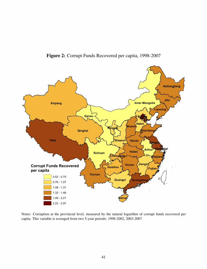
Figure 2: Corrupt Funds Recovered per capita, 1998-2007

Tibet

Xinjiang

Qinghai

Inner Mongolia

Sichuan

Gansu

Yunnan

Jilin

Hunan

Heilongjiang

Hubei

Hebei

Guangxi

HenanShaanxi

Jiangxi

Anhui

Guizhou Fujian

Guangdong

Liaoning

ShanxiShandong

Jiangsu

ZhejiangChongqing

Ningxia

Hainan

BeijingTianjin

Shanghai

Corrupt Funds Recoveredper capita

0.52 - 0.750.76 - 1.071.08 - 1.311.32 - 1.481.49 - 2.212.22 - 2.97

Notes: Corruption at the provincial level, measured by the natural logarithm of corrupt funds recovered percapita. This variable is averaged from two 5-year periods: 1998-2002, 2003-2007.

41

Figure 3: Senior Cadres Disciplined per 10,000 Public Employees, 1998-2007

Tibet

Xinjiang

Qinghai

Inner Mongolia

Sichuan

Gansu

Yunnan

Jilin

Hunan

Heilongjiang

Hubei

Hebei

Guangxi

HenanShaanxi

Jiangxi

Anhui

Guizhou Fujian

Guangdong

Liaoning

ShanxiShandong

Jiangsu

ZhejiangChongqing

Ningxia

Hainan

BeijingTianjin

Shanghai

Senior Cadres Disciplinedper 10,000 Public Employees

-1.87 - -1.39-1.38 - -1.16-1.15 - -0.81-0.80 - -0.45-0.44 - -0.06

Notes: Corruption at the provincial level, measured by the natural logarithm of senior cadres disciplined per10,000 public employees. This variable is averaged from two 5-year periods: 1998-2002, 2003-2007.

42

7 Appendix

7.1 Does Country of Origin Matter?

In the paper, I have shown that MNC activities increase corruption in China. In the analyses, all FDI

originated from different countries are assumed to have the same impact. In China, a substantial part

of FDI is actually from Hong Kong, Macao and Taiwan (HMT). HMT investors are supposed to be

more familiar with the business practices in China and have more connections with local governments.

Thus We may wonder whether HMT investors behave differently from others. It could be the HTM

FDI that actually drives the positive relationship between MNC activities and corruption. To examine

whether HTM FDI really makes a difference, I disaggregate FDI into HTM and non-HTM origins. To

be consistent with previous results, I again average both variables for two 5-year periods: 1998-2002

and 2003-2007. Since data on FIE trade by partner countries at the provincial level is not available,

MNC activities are measured by inward FDI from either the HTM or non-HTM region as a percentage

of GDP. The dependent variable is the three corruption measures based on filed cases. Given the

high collinearity between these two FDI variables (R=0.91), they enter into the regression equation

separately. To deal with possible endogeneity, both variables are lagged one period. As shown before,

OLS regression tends to underestimate the coefficient of MNC activities. If we observe a positive

and significant coefficient in OLS regressions, the true coefficient will be larger when endogeneity is

accounted for. Results are presented in Table A.

We can see that both HTM and non-HTM FDI are positively and strongly associated with the three

measures of corruption. The substantive effects of these two variables are not significantly different.

For instance, in Models 1 and 2 in Table A, one standard deviation change in HTM FDI will increase

corrupt funds recovered per filed case by U12,591 ($2,078), while the same change in non-HTM FDI

will do so by U12,681 ($2,093). It seems that FDI originated from both HMT and non-HMT regions

contributes to corruption in China. One caveat of these results is that FDI data by country of origin

at the provincial level is less reliable as the reporting procedure has changed over time and some

provinces do not distinguish between foreign capital and foreign direct investment. The results are

more suggestive rather than conclusive.

1

7.2 Sensitivity Analysis of IV Exclusion Restriction

A valid instrumental variable requires that it effects the dependent variable only through the endoge-

nous variable. A potential violation of the exclusion restriction presents one challenge to the iden-

tification. In this case, geographic distance impacts corruption through the activities that are related

to distance. We have reason to believe that geographic distance has an effect on corruption primarily

through the two major transnational economic activities – foreign investment and trade. However, it is

possible that geographic closeness influences corruption through labor movement, migration, or even

the media. This kind of effects should be at margin because cross-border labor movement and migra-

tion are still limited in China and the government highly restricts foreign media. In addition, Hong

Kong, Japan, Korea, Singapore and Taiwan are all considered to be less corrupt than China.1 Thus

we should expect a negative effect of geographic closeness on corruption through labor movement,

migration, and foreign media. If this is the case, the 2SLS models tend to underestimate the positive

coefficient of MNC activities on corruption. Nonetheless, we might still worry that geographic close-

ness has an impact on corruption in some unobservable ways and thus the exclusion restriction could

be violated.

As suggested by Conley et al. (2012), I preform a sensitivity analysis to assess to what extent the

empirical results are sensitive to the possible violation of the exclusion restriction. The model can be

set up as follows:2

Y = Xβ + Zγ + ε (1)

X = Zλ+ υ (2)

Where Z is the (excluded) instrument (geographic closeness) for the endogenous variable of X

(MNC activities); E(Xε) 6= 0 andE[Zε] = 0. γ is a parameter measuring to what extent the exclusion

restriction is satisfied. In a normal setup, the term – Zγ – does not appear in the structural equation

(1). If the exclusion restriction holds, then γ = 0. We can estimate the two equations using a normal

1According to the TI, for instance, in 2007 the corruption perceptions indices (CPI) of Hong Kong, Japan, Korea,Singapore and Taiwan were 8.3, 7.5, 5.1, 9.3, and 5.7 respectively. China’s CPI was 3.5 which was far below the fiveeconomies’ CPIs.

2See, Conley et al. (2012, 261).

2

2SLS regression. If the exclusion restriction is violated, γ 6= 0. Based on these two equations, we can

conduct a sensitivity analysis using the prior knowledge about the magnitude of γ.

In this case, we are more interested in the positive values of γ, because a negative γ will increase

the slope of MNC activities. I focus on two of the approaches recommended by Conley et al. (2012).

The first approach is to specify a set of values for γ based on prior knowledge and obtain a union of

confidence intervals for β. I want to see how large the γ could be so that we still obtain a signifi-

cant positive coefficient of MNC activities at the 90% level.3 The second approach is “local-to-zero

approximation” that adopts a large sample approximation and treats the uncertainty of γ as sample

uncertainty to obtain an approximate distribution for β (Conley et al. 2012, 264-65). This approach

allows the levels of confidence intervals of β to depend on the probabilities of observing specific val-

ues of γ.4 Since we have reason to believe geographic closeness affects corruption primarily through

the channels of inward FDI and trade, γ should be small even if the exclusion restriction is violated.

Thus, I choose a normal distribution for γ with a mean of 0 and a variance of σ2 to capture the fact

that there is a high probability of observing γ = 0. I conduct the sensitivity analysis on Model 7 in

Table 1 and Models 5 and 10 in Table 2. Results are presented in Table B.

In Approach 1, we can see here that γ can be as large as 0.41, 0.22 and 0.035 in these three

models, we still observe a positive and significant effect of MNC activities on corruption. The point

estimates of MNC activities are 0.17, 0.16 and 0.14 respectively. After we subtract the direct effect

of geographic closeness on corruption, all else being equal, one standard deviation increase in MNC

activities will still raise corrupt funds recovered per filed case by U11,853 ($ 1,956), corrupt funds

recovered per capita by U1.17 ($ 0.18), and senior cadres disciplined per 10,000 public employees

by 1.13 units. The effects are substantively large. These results indicate that MNC activities affect

3We are more interested in positive values of γ. If γ is negative, a normal 2SLS regression in fact underestimates thecoefficient of MNC activities.

4In the case of a Gaussian prior for γ, βapprox ∼ N(β + Aµγ , V2SLS + Aσ2γA′), and A =

(X ′Z(Z ′Z)−1Z ′X)−1(X ′Z), where β and V2SLS are the point estimates and variance-covariance matrix obtained froma normal 2SLS regression; µγ and σ2

γ are the mean and variance of the prior distribution of γ; X and Z are the endogenousand instrumental variables respectively. See, Conley et al. (2012, 264).

5If these numbers were the true coefficients of geographic closeness in equation 1, one standard deviation increase ingeographic closeness would raise recovered corrupt funds per filed case by U11,720 ($1,934), recovered corrupt funds percapita by U1.09 ($0.18), and senior cadres disciplined per 10,000 public employees by 1.01 units when all other variablesare held constant. These numbers would represent considerably large effects of geographic closeness on corruption.

3

corruption positively and significantly even if we allow for a considerable deviation from the perfect

instrumental variable. Next, I draw γ from prior normal distributions in which σ= 0.25, 0.15 and 0.03

for Model 7 in Table 1 and Models 5 and 10 in Table 2 respectively.6 Again, we can see that even if

we take into account the uncertainty about γ, the 90% confidence interval of the coefficient of MNC

activities is still above 0 in all three models. This finding confirms that the positive effect of MNC

activities on corruption is not sensitive to the potential violation of the exclusion restriction.

6If these three numbers were the true coefficients of geographic closeness, all else being equal, one standard deviationincrease in geographic closeness would raise recovered corrupt funds per filed case by U11,016 ($1,818), recovered corruptfunds per capita by U1.06 ($0.18), and senior cadres disciplined per 10,000 public employees by 1.01 units. In fact, weallow γ to vary beyond σ. Approximately 95% of the γ values range between −2σ and 2σ.

4

7.3 Firm-Level Variables in Table 4

• SOE: a dummy variable coded as 1 if firms are registered as state-owned and the share of state

capital is larger than 50%, 0 otherwise.

• Collective: a dummy variable coded as 1 if firms are registered as collective-owned and the

share of collective capital is larger than 50%, 0 otherwise.

• Private: a dummy variable coded as 1 if firms are registered as private-owned and the share of

private capital is larger than 50%, 0 otherwise.

• Foreign (HK, MC, TW): a dummy variable coded as 1 if firms are registered as foreign-owned

(Hong Kong, Macao, and Taiwan) and the share of foreign capital is larger than 50%, 0 other-

wise.

• Foreign (Other Countries): a dummy variable coded as 1 if firms are registered as foreign-

owned (other than Hong Kong, Macao, and Taiwan) and the share of foreign capital is larger

than 50%, 0 otherwise.

• Revenue (log): log of total business income (core business income + other business income) in

2004

• Sales to government: % of sales to government in 2004.

• Sales to SOEs: % of sales to SOEs in 2004.

• License: the number of licenses and registrations (permanent and renewable annually) required

for firms.

• Interaction with government: the number of days that firms’ general manager (GM) or vice

GM spend on the government assignments and communications.

• R&D: expenditures on R&D, % of total revenue in 2004. ”

• Skill intensity: the ratio of employees with college education or above.

5

Table A: Hong Kong, Macao and Taiwan FDI vs Other FDI

(1) (2) (3) (4) (5) (6)HMT FDI 0.24*** 0.23*** 0.17***

(0.08) (0.07) (0.06)Non-HMT FDI 0.20** 0.19** 0.16**

(0.10) (0.09) (0.07)GDP per capita (log) -0.83* -0.96* -0.26 -0.39 -0.16 -0.35

(0.43) (0.48) (0.30) (0.36) (0.29) (0.30)GDP 0.04 0.05 0.02 0.03 0.01 0.02

(0.03) (0.03) (0.02) (0.02) (0.02) (0.02)Government Expenditure 0.72* 0.79* 0.14 0.19 0.15 0.23(% GDP, log) (0.37) (0.41) (0.32) (0.35) (0.26) (0.28)Public Employees 8.49 5.67 15.54*** 12.72** -0.29 -2.02

(5.06) (6.00) (4.69) (4.83) (3.49) (3.97)Time 0.07 -0.08 0.59 0.44 0.20 0.08

(0.58) (0.60) (0.51) (0.54) (0.28) (0.32)Bureaucratic Integration 0.13 0.11 0.08 0.06 -0.05 -0.07

(0.10) (0.11) (0.07) (0.08) (0.05) (0.05)Dummy of Four Municipalities 0.56** 0.57** 0.35** 0.37** 0.81*** 0.84***

(0.21) (0.23) (0.16) (0.18) (0.28) (0.28)Trust in Courts 0.38 0.38 0.57 0.56 0.02 -0.03

(0.42) (0.44) (0.38) (0.40) (0.18) (0.16)Schooling 0.39 0.56 -0.24 -0.06 -0.06 0.12

(0.58) (0.61) (0.47) (0.49) (0.36) (0.39)Relative Wages 0.37 0.28 0.14 0.06 0.47** 0.45*

(0.33) (0.38) (0.27) (0.32) (0.18) (0.22)Gender 4.20 5.82 4.24 5.79 -1.39 0.32

(4.90) (4.67) (3.75) (3.81) (3.24) (3.00)Constant 3.77 4.09 -1.72 -1.42 0.09 0.77

(3.92) (4.29) (2.86) (3.27) (2.38) (2.46)N 44 45 44 45 43 44R2 0.54 0.52 0.61 0.58 0.71 0.69Notes: Robust standard errors in parentheses;* significant at 10%, ** significant at 5%; *** significant at 1%.

6

Table B: Sensitivity Analysis of the IV Exclusion Restriction of Model 7 in Table 1and Models 5 & 10 in Table 2

Dependent VariableCorrupt Funds Recovered Corrupt Funds Recovered Senior Cadres Disciplined

Per Filed Case Per Capita Per 10,000 Public Employees

Approach 1

Maximum γ for0.41 0.22 0.03

a Significant β

Point Estimate β 0.17 0.16 0.14(MNC Activities)

90% Confidence Interval [0.00, 0.33] [0.00, 0.31] [0.00, 0.28]

Approach 2

Prior Distribution of γ γ ∼ N(0, 0.252) γ ∼ N(0, 0.152) γ ∼ N(0, 0.032)

Point Estimate β0.47 0.32 0.17

(MNC Activities)

90% Confidence Interval [0.10, 0.84] [0.07, 0.60] [0.00, 0.33]

7

Table C: First Stage Regressions of Models in Table 1

Model (2a) (3a) (4a) (5a) (6a) (7a)Geographic Closeness 1.34*** 1.35*** 1.35*** 1.31*** 1.35*** 1.33***

(0.17) (0.18) (0.17) (0.17) (0.18) (0.18)GDP per capita (log) 1.10*** 1.10*** 0.99*** 1.08*** 0.97*** 0.66**

(0.18) (0.18) (0.23) (0.17) (0.22) (0.28)GDP -0.02 -0.02 -0.02 -0.03 -0.02 -0.00

(0.02) (0.02) (0.02) (0.02) (0.02) (0.02)Government Expenditure -0.86*** -0.86*** -0.81*** -1.02*** -0.95*** -0.78***(% GDP, log) (0.18) (0.18) (0.19) (0.22) (0.24) (0.25)Public Employees -1.37 -1.14 -0.97 -0.14 0.58 -1.21

(3.47) (3.54) (3.52) (3.37) (3.49) (4.95)Time -0.00 0.00 -0.00 0.23 0.22 -0.19

(0.14) (0.14) (0.14) (0.15) (0.16) (0.30)Bureaucratic Integration -0.03 -0.06 -0.08

(0.07) (0.08) (0.08)Four Municipalities 0.19 0.22 0.24

(0.23) (0.25) (0.26)Trust in Courts 0.46** 0.46** 0.33

(0.20) (0.21) (0.22)Schooling 0.50

(0.37)Relative Wages 0.51

(0.33)Gender -2.46

(3.38)Constant -13.73*** -13.74*** -13.14*** -15.49*** -14.87*** -12.40***

(1.00) (1.01) (1.24) (1.26) (1.51) (2.12)N 61 61 61 55 55 55R2 0.84 0.84 0.85 0.85 0.85 0.87F − Statistic

59.59 58.61 59.85 59.43 57.58 53.62(Excluded Instrument)Notes: Standard errors in parentheses* significant at 10%, ** significant at 5%; *** significant at 1%

8

Table D: Descriptive Statistics

Variable Obs Mean Std. Dev. Min MaxCorrupt Funds Recovered Per Filed Case (log) 61 2.55 0.68 0.93 4.60Corrupt Funds Recovered Per Capita (log) 61 1.34 0.62 0.07 3.00Senior Cadres Disciplined Per 10,000 Public Employees (log) 60 -1.03 0.41 -2.08 0.10Frequency of Witnessed Corruption 26 0.13 0.07 0 0.25Level of Perceived Corruption 26 2.44 0.21 1.96 2.81MNC Activities (Factor Score) 61 -0.02 1.00 -1.60 1.96GDP per capita (log) 61 5.68 0.55 4.83 7.63GDP 61 8.26 5.37 0.40 22.18Government Expenditure (% GDP, log) 61 -2.14 0.47 -2.95 -0.49Public Employees (Proportion to Population) 61 0.06 0.03 0.03 0.19Time 61 0.51 0.50 0 1Dummy of Four Municipalities 61 0.13 0.34 0 1Bureaucratic Integration 61 2.37 0.89 1 4Trust in Courts 55 3.19 0.28 2.38 3.93Schooling 61 1.50 0.62 -0.27 3.24Public Employees’ Relative Wages 61 1.11 0.20 0.77 1.96Gender (Share of Female Public Employees) 61 0.37 0.02 0.33 0.43

9

Tabl

eE

:Cor

rela

tion

Mat

rix

ofE

xpla

nato

ryV

aria

bles

Var

iabl

esM

NC

GD

PG

DP

Gov

ernm

ent

Publ

icTi

me

Bur

eauc

ratic

Dum

my

ofTr

usti

nSc

hool

ing

Rel

ativ

eG

ende

rA

ctiv

ities

perc

apita

Exp

endi

ture

Em

ploy

ees

Con

trol

Mun

icip

aliti

esC

ourt

sW

ages

MN

C1.

00A

ctiv

ities

GD

P0.

591.

00pe

rcap

ita

GD

P0.

520.

401.

00

Gov

ernm

ent

-0.3

90.

13-0

.45

1.00

Exp

endi

ture

Publ

ic0.

160.

63-0

.08

0.12

1.00

Em

ploy

ees

Tim

e0.

150.

180.

270.

35-0

.33

1.00

Bur

eauc

ratic

0.35

0.36

0.35

-0.1

10.

170.

111.

00C

ontr

olD

umm

yof

0.42

0.65

0.05

0.03

0.48

0.01

0.47

1.00

Mun

icip

aliti

esTr

usti

n0.

00-0

.13

-0.1

5-0

.16

0.09

-0.3

7-0

.06

0.01

1.00

Cou

rts

Scho

olin

g0.

560.

850.

320.

210.

530.

500.

340.

56-0

.17

1.00

Rel

ativ

e0.

15-0

.10

0.04

0.01

-0.3

90.

360.

08-0

.11

0.14

0.06

1.00

Wag

es

Gen

der

0.27

0.37

0.14

0.02

0.31

0.12

0.18

0.13

0.17

0.45

0.14

1.00

10