mobile 3d visual search based on local stereo image features
TRANSCRIPT

Master Thesis
Mobile 3D Visual Search based onLocal Stereo Image Features
Hequn BAI
Stockholm, Sweden 2012
XR-EE-SIP 2012:004

Mobile 3D Visual Search based on
Local Stereo Image Features
HEQUN BAI
Master Thesis
School of Electrical Engineering
August 2012

AbstractMany recent applications using local image features focus on 2D imagerecognition. Such applications can not distinguish between real objectsand photos of objects. In this project, we present a 3D object recognitionmethod using stereo images. Using the 3D information of the objectsobtained from stereo images, objects with similar image description butdifferent 3D shapes can be distinguished, such as real objects and pho-tos of objects. Besides, the feature matching performance is improvedcompared with the method using only local image features. Knowingthe fact that local image features may consume higher bitrates thantransmitting the compressed images itself, we evaluate the performanceof a recently proposed low-bitrate local image feature descriptor CHoGin 3D object reconstruction and recognition, and propose a differencecompression method based on the quantized CHoG descriptor, whichfurther reduces bitrates.
Contents
1 Introduction 1
2 Background 3
3 3D Visual Search 5
3.1 3D Reconstruction from Stereo Images . . . . . . . . . . . . . . . . . 5
3.2 Stereo Keypoint Matching using SIFT . . . . . . . . . . . . . . . . . 8
3.3 3D Feature Matching . . . . . . . . . . . . . . . . . . . . . . . . . . . 10
3.4 Construction of Planar Models . . . . . . . . . . . . . . . . . . . . . 12
3.4.1 Fitting of 3D Points . . . . . . . . . . . . . . . . . . . . . . . 12
3.4.2 Planar Model . . . . . . . . . . . . . . . . . . . . . . . . . . . 13
3.4.3 Matching of Planar Model . . . . . . . . . . . . . . . . . . . . 15
4 Compression of 3D Features 17
4.1 Compressed Histogram of Gradients . . . . . . . . . . . . . . . . . . 17
4.2 Difference Coding of Descriptors . . . . . . . . . . . . . . . . . . . . 18
5 Experimental Results 23
5.1 Experimental Setup . . . . . . . . . . . . . . . . . . . . . . . . . . . 23
5.2 Stereo Images Synthesis . . . . . . . . . . . . . . . . . . . . . . . . . 24
5.3 Experiments using SIFT . . . . . . . . . . . . . . . . . . . . . . . . . 25
5.3.1 Verification of Distances . . . . . . . . . . . . . . . . . . . . . 25

5.3.2 Construction of Planar Model . . . . . . . . . . . . . . . . . . 26
5.4 Experiments using CHoG . . . . . . . . . . . . . . . . . . . . . . . . 29
5.4.1 Discriptor Differences . . . . . . . . . . . . . . . . . . . . . . 29
5.4.2 Recognition Rate . . . . . . . . . . . . . . . . . . . . . . . . . 30
6 Conclusions 33
Bibliography 35

Chapter 1
Introduction
Recently local image features have been of wide interest in computer vision.These features are extracted using the information from local pixels around theinterest point, such as colors and gradient of intensity, and are used to distinguishbetween different points among images. Such local features can be used to do taskssuch as identifying books, DVDs or print media. However since these applicationsare based on two dimensional (2D) image registration, they can not distinguishbetween real objects and photos of objects. For example, if we take a photo of areal building and another photo of the picture of the building, 2D image recognitionsystems will extract similar local image features and give the same recognitionresults.
Stereo images, by combining the information from two 2D images taken in differ-ent viewpoints, can jointly reconstruct the 3D shape of the object. In this report wedescribe the approach of 3D information reconstruction using SIFT [1] local imagefeatures. The 3D information is represented by the distances between feature pointsand angles between surfaces of the object. With the help of such 3D information,the local image features can be used for recognition of 3D objects. The experimentalresults show that in addition of being able to distinguish between real objects andphotos of objects, such 3D information also increases the discrimination ability ofthose feature points because the 3D information carried by the feature points onone object are sometimes quite unique from the 3D information carried by otherobjects.
Since the SIFT descriptor is of 128 dimensions, the data size of storing the SIFTfeatures are usually even larger than storing the compressed image using JEPG.The recently proposed low-bitrate local image feature, Compressed Histogram ofGradients [2] (CHoG), achieves a 10× to 20× reduction in bitrate compared with theSIFT descriptor. In this project we evaluate its performance in 3D reconstructionand 3D object recognition using different binning schemes. Observing that there
1
CHAPTER 1. INTRODUCTION
exist similarities among CHoG descriptors within an image, we use difference codingto compress the CHoG descriptor even further. The experiments show that thebitrate can be reduced by 10% - 35% by using difference compression.
The report is arranged as follows. In Chapter 2, we review recent techniqueson 2D and 3D object recognition. In Chapter 3, we use SIFT features for 3Dreconstruction and feature description. The algorithm of constructing planar modelsfor describing surfaces of objects with planes will be present. We use 3D distancesand 3D angles to verify the point matches and distinguish between objects andtheir photos. In Chapter 4, we take advantage of the similarities among CHoGdescriptors within an image and presents difference compression method to furtherreduce the bitrate. We give the experimental results on recognizing 3D objects inChapter 5. Both the feature-level matching performance using 3D information andthe recognition rate for distinguishing real objects and their photos will be given.Some potential limitations are discussed in this chapter. In Chapter 6, the resultsof the whole project are concluded and future work is discussed.
2
Chapter 2
Background
Several local image descriptors have been proposed in recently years, includingthe most famous SIFT feature and Speeded Up Robust Feature [3] (SURF). TheSIFT descriptor, since its proposition in 1999, has been widely used in video tracking[4], 3D reconstruction [5] and object registeration [6][7]. It detects keypoints byusing scale-space extrema in the difference-of-Gaussian function convolved with theimage. The descriptor is formulated to present the gradient magnitude at differentdirections around the keypoint. The SIFT descriptor is of 128 dimensions with 4×4subregions and 8 directions within each subregion. The match for each keypoint isdone by finding the keypoint with minimum Euclidean distance in the database.
The 128 dimensional SIFT descriptor is normally stored in 1024 bits, using 8bits per dimension. Because of the high bitrate of the SIFT descriptor, the datasize of all the SIFT descriptors extracted from an image is usually much larger thanthe size of the original image compressed using JPEG. Thus the SIFT feature isnot suitable for applications which require to transmit the descriptors via wirelessnetworks. Many compression methods have been proposed after the propositionof SIFT, including Locality Sensitive Hashing [8], Similarity Sensitive Hashing [9],transform coding [10] and the most commonly used Vector Quantization [11]. In [12]the authors give a comparison of these compression schemes for the SIFT descriptor.
A low-bitrate local image feature, Compressed Histogram of Gradients (CHoG),was proposed in [2]. The low bitrate of the new descriptor is achieved by designingthe descriptor with compact spatial binning and gradient binning schemes. Insteadof using a square 4 × 4 grid with 16 cells as used in SIFT and SURF descriptors,CHoG divides the patch into log-polar configurations. The gradient histogram bin-ning schemes are designed to have a central bin at the origin and the remainingbins are evenly spaced over an ellipse. Such a scheme can capture both the centralpeak of the gradient distribution and the gradients in different directions withinthat patch. The histogram quantization and compression is done by using Huffman
3
CHAPTER 2. BACKGROUND
tree coding and type coding.
[13] evaluates the performance of MPEG-7 image signatures, CHoG and SIFTdescriptors in both feature-level matching and image-level matching. The resultsshow that the CHoG descriptor has a comparable bitrate to MPEG-7 image signa-tures while outperforming MPEG-7 image signatures in terms of feature matchingperformance. With the low bitrate feature descriptors, [14] discusses the systemdesign issues for mobile visual search applications using local image features. Sev-eral client-server modes are discussed. In the client-server mode, it is shown thatby using CHoG features the transmission delay is significantly reduced in wirelessnetworks compared with transmitting SIFT features or JPEG pictures. In orderto speed up the recognition process, it uses a fast geometric reranking algorithmto give a short list of candidate images before running RANSAC [15] geometricverification.
The above systems can only recognize 2D images. For describing 3D surfaces,[16] uses spin images to relate the neighboring points of a feature to the normalvector of the feature. The three dimensional information is then mapped into a2D histogram. The coordinates of this histogram are distance along the feature’snormal vector and radial distance from the normal vector, with the feature locationas the origin. [17] takes advantage of the idea from SIFT features and improves thespin image descriptor to be rotation invariant. Other 3D surface descriptors includepairwise geometric histograms [18] and Extended Gaussian Images [19]. These 3Ddescriptors rely on the availability of dense points in 3D.
Some work has been done by using local image features for 3D object recog-nition. [7] uses a view clustering approach to integrate several images taken fromdifferent viewpoints of an object into a single model. It uses a similarity transformto map the feature points between images from different viewpoints and to linkthe matched feature points between views. At the recognition procedure, insteadof using just the number of feature matches, it uses a probability model for ver-ification, where it accepts a model interpretation if the likelihood of the presenceis higher than 0.95. [20] uses local affine-invariant descriptors to represent the 2Dimage features and uses spatial relationships to link feature points from differentviews. Geometric constraints associated with different views of the same featurepoint are combined. The appearance of the feature points is normalized, and guidesmatching and reconstruction together with the geometric information. This allowsrecognizing photographs taken from arbitrary viewpoints.
Although [7] and [20] construct 3D models to constrain the geometric relation-ship of feature points, they still use a 2D photograph as a query image. Thus theyare still not capable to distinguish between real objects and photos of objects.
4
Chapter 3
3D Visual Search
2D image recognition methods have the disadvantage that they cannot distin-guish between photos of the object and the object itself. It can also be fooled bya scaled model of the real 3D object. Besides, such systems can not cope with sit-uations when the viewpoint changes. Current solutions to viewpoint changes storemultiple images taken from different viewpoints of the object. This requires a largedatabase of overlapping images taken from densely placed viewpoints. This chapterwill describe a solution for 3D object recognition, using stereo cameras to extractthe 3D information of the object. 3D locations are calculated by using matchedpoints found by SIFT features from stereo images. An algorithm for constructingplanar models is developed, which is suitable for objects with planar surfaces, suchas buildings. The 3D information, such as the surface normals of planar surfacesand distances between feature points will be used to verify the point matches foundby local image features.
3.1 3D Reconstruction from Stereo Images
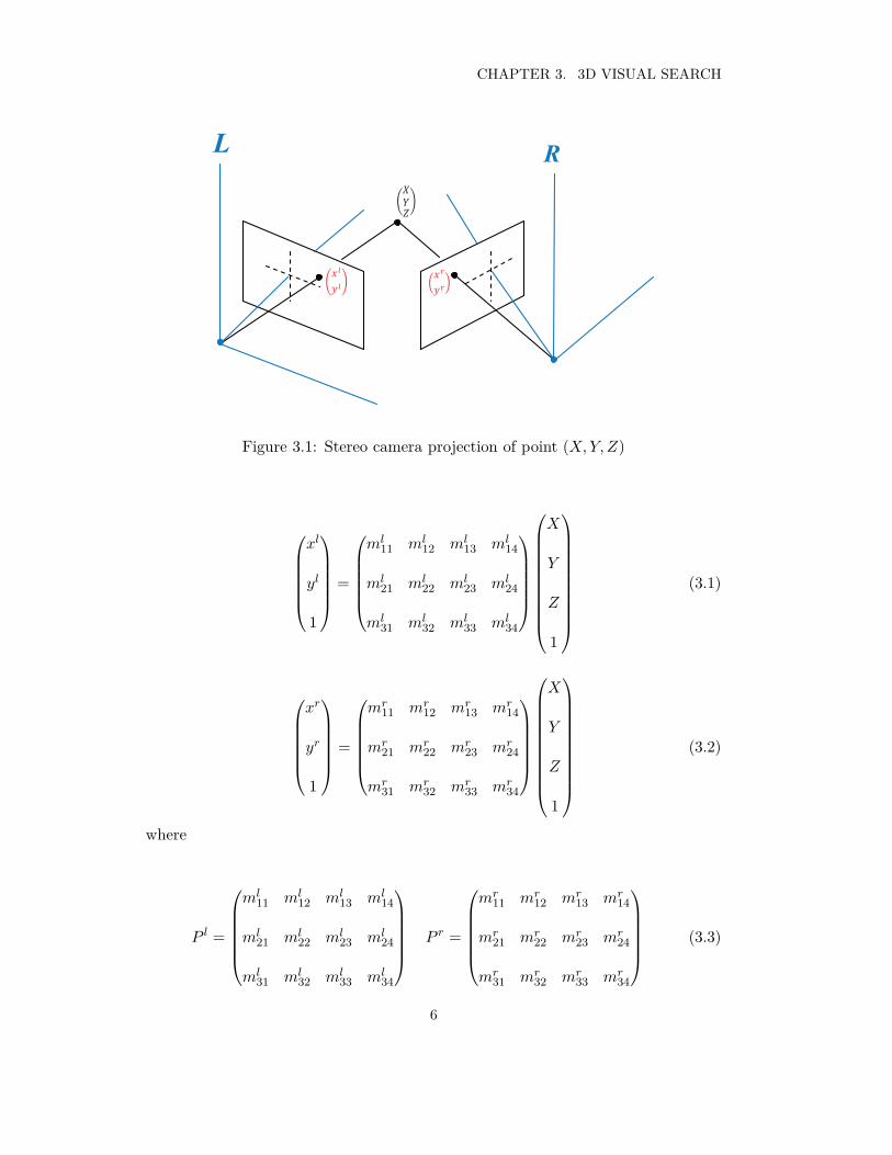
When taking photos with a camera, the 3D information of the object is lostwhen the 3D object is projected on the 2D image plane. If we have more than twocameras with known camera parameters, as shown in Figure 3.1, the 3D location ofthe points on the object can be recovered using the pixel correspondence betweenthe stereo images L and R. Let the coordinates of the point in 3D space be (X, Y, Z)and the coordinates of its corresponding projection points in left and right imagesbe (xl, yl) and (xr, yr), then we have the following relations
5
CHAPTER 3. 3D VISUAL SEARCH
!"&$&% '"($()
!*+,%
LR
Figure 3.1: Stereo camera projection of point (X, Y, Z)
xl
yl
1
=
ml11 ml
12 ml13 ml
14
ml21 ml
22 ml23 ml
24
ml31 ml
32 ml33 ml
34
X
Y
Z
1
(3.1)
xr
yr
1
=
mr11 mr
12 mr13 mr
14
mr21 mr
22 mr23 mr
24
mr31 mr
32 mr33 mr
34
X
Y
Z
1
(3.2)
where
P l =
ml11 ml
12 ml13 ml
14
ml21 ml
22 ml23 ml
24
ml31 ml
32 ml33 ml
34
P r =
mr11 mr
12 mr13 mr
14
mr21 mr
22 mr23 mr
24
mr31 mr
32 mr33 mr
34
(3.3)
6
3.1. 3D RECONSTRUCTION FROM STEREO IMAGES
are known calibrated camera projection matrices of left and right views, which arethe product of the corresponding internal camera parameter, rotation matrix and ascaling factor for each view.
With the calibrated projection matrices of left and right views, the 3D coordi-nates (X, Y, Z) can be computed. From Eq.(3.1) and Eq.(3.2) we can have
xl =ml
11X + ml12Y + ml
13Z + ml14
ml31X + ml
32Y + ml33Z + ml
34
(3.4)
yl =ml
21X + ml22Y + ml
23Z + ml24
ml31X + ml
32Y + ml33Z + ml
34
(3.5)
xr =mr
11X + mr12Y + mr
13Z + mr14
mr31X + mr
32Y + mr33Z + mr
34
(3.6)
yr =mr
21X + mr22Y + mr
23Z + mr24
mr31X + mr
32Y + mr33Z + mr
34
(3.7)
These four equations above can be rearranged as
(xlml31 − ml
11) (xlml32 − ml
12) (xlml33 − ml
13) (xlml34 − ml
14)
(xlml31 − ml
21) (xlml32 − ml
22) (xlml33 − ml
23) (xlml34 − ml
24)
(xrmr31 − mr
11) (xrmr32 − mr
12) (xrmr33 − mr
13) (xrmr34 − mr
14)
(xrmr31 − mr
21) (xrmr32 − mr
22) (xrmr33 − mr
23) (xrmr34 − mr
24)
XYZ1
= 0.
(3.8)
There are four linear equations with three unknowns. Thus (X, Y, Z) will becomputed by solving the set of over-determined equations. We rewrite Eq.(3.8) ina compact form
Ax = 0 (3.9)
where
7
CHAPTER 3. 3D VISUAL SEARCH
A =
(xlml31 − ml
11) (xlml32 − ml
12) (xlml33 − ml
13) (xlml34 − ml
14)
(xlml31 − ml
21) (xlml32 − ml
22) (xlml33 − ml
23) (xlml34 − ml
24)
(xrmr31 − mr
11) (xrmr32 − mr
12) (xrmr33 − mr
13) (xrmr34 − mr
14)
(xrmr31 − mr
21) (xrmr32 − mr
22) (xrmr33 − mr
23) (xrmr34 − mr
24)
(3.10)
x =
XYZ1
. (3.11)
This is a homogeneous system of equations that can be solved by using the leastsquares method. The least squares solution x = (x1, x2, x3, x4)T is the eigenvectorof AtA with the minimum eigenvalue. The method on how to solve Eq.(3.9) is in[21]. The 3D coordinates of the point (X, Y, Z) can be obtained by normalizing xby x4.
XYZ1
=
x1/x4
x2/x4
x3/x4
x4/x4
(3.12)
3.2 Stereo Keypoint Matching using SIFT
As seen in Section 3.1, in order to get the 3D location of feature points (X, Y, Z),we need the coordinates of the corresponding points (xl, yl) and (xr, yr) in theleft and right images. Since the SIFT descriptor is highly discriminative in pointmatching, we use the SIFT algorithm to find keypoints and match correspondingfeature points between left and right images. We refer to the matching of keypointsin the left and right images as stereo keypoint matching.
The SIFT feature is a statistical representation of local image gradients. Foran image L(x, y), at each pixel around the keypoint, the magnitude of the gradientm(x, y), and the orientation r(x, y) are computed as follows.
m(x, y) =√
(L(x + 1, y) − L(x − 1, y))2 + (L(x, y + 1) − L(x, y − 1))2 (3.13)
r(x, y) = tan−1((L(x, y + 1) − L(x, y − 1))/(L(x + 1, y) − L(x − 1, y))) (3.14)
8
3.2. STEREO KEYPOINT MATCHING USING SIFT
Around each keypoint, the image is divided into 4 × 4 grid subregions. Ineach subregion, the gradient directions are quantized into 8 direction bins and theaccumulative gradient magnitude in each direction bin is stored as a description ofgradient statistics in that direction. This forms a feature vector of 128 dimensionsin total. We use such a descriptor to match the keypoints between the left and rightimages, as well as between query images and the images in the database.
SIFT features have the following additional characteristics that make it suitablefor our application of 3D object recognition.
1. Keypoints are detected by computing the local extrema in the image domainand the scale domain such that the keypoints are invariant to image scaling.
2. The orientation of each feature is determined by the dominant direction in thehistogram of gradients such that the feature descriptor is invariant to imagerotation.
3. The keypoint locations are refined to subpixel accuracy, by using a Taylorexpansion of the scale-space function and setting the derivative of the functionto zero. The increased accuracy of matched point locations in left and rightimages makes the 3D location reconstruction more accurate.
Stereo keypoint matching is done by finding the nearest neighbor of the featurevector. The nearest neighbor is defined by the feature vector with minimum Eu-clidean distance. For the keypoint i with feature descriptor Dl
i in the left image, itsmatched keypoint j with feature descriptor Dr
jin the right image is found by
j = argminj
‖Dli − Dr
j ‖2, (3.15)
where Dli and Dr
j are vectors of 128 dimensions.
However, some keypoints may have several similar matches, such as repeatedwindows and similar patterns on the wall. It is easy in this case to have an incorrectmatch by only finding the nearest neighbor in feature vectors. Some other keypoints,usually coming from the background, are not very discriminative and can be easilymatched to some other background patches. In [1], Lowe uses the ratio between thedistance to the closest feature vector and the distance to the second closest featurevector. A threshold θ1 is used to discard those matches whose ratio is close to 1.
This method is important to discard incorrect matches in 2D image recognition.The proposed ratio is between 0.7 and 0.8, which considerably eliminates incorrectmatches, but at the same time, rejects also some correct matches. In our applicationcase of stereo matching, since the locations of the matched points will be used for 3Dreconstruction and as the 3D reconstruction method has another threshold to rejectincorrect matches, we simply relax the threshold here to include more matchedpairs. More incorrect matches are discarded at the 3D reconstruction stage.
9
CHAPTER 3. 3D VISUAL SEARCH
Suppose the 3D coordinates calculated from Eq.(3.12) is (X, Y , Z). Using theprojection matrix denoted in Eq.(3.1) and Eq.(3.2), the locations of the correspond-ing camera projection points in the left and right images can be calculated and nor-malized. The keypoint locations in the left and right images are denoted as (xl, yl)and (xr, yr). Because of imperfectness in camera calibration and limited localizationaccuracy of matched points in the left and right images, there exist errors between(xl, yl) (xr, yr) and (xl, yl) (xr, yr). The square error can be expressed as
e = ‖(xl, yl) − (xl, yl)‖2 + ‖(xr, yr) − (xr, yr)‖2 (3.16)
Since the keypoint localization using the SIFT algorithm is at subpixel accuracy,and taking into account the imperfectness of the camera projection parameters,the difference between the returned keypoint locations and the original keypointlocations given by the SIFT algorithm should be smaller than a threshold θ, wherewe set θ = 1 for the SIFT features in the later experiments. Matched pairs, forwhich e > θ holds, are very likely to result from incorrect matched pairs and thusare discarded. This method is equivalent to thresholding the minimum eigenvalueof the matrix AtA in Eq.(3.9). We use this approach to eliminate incorrect matches.
3.3 3D Feature Matching
2D image recognition systems use some robust regression techniques, such asRANSAC [15] and the Hough Transform [6], to verify the keypoints such that theyagree upon a particular model pose. In [14] a fast geometric reranking algorithmis used, which calculates the 2D distance between pairs of features within an im-age, and computes the log-distance ratio between corresponding pairs. It uses thepeak value in the histogram of the log-distance ratio to represent the geometricconsistency.
In 3D object recognition we can easily obtain the true 3D distances betweenfeature points from the stereo images. The distances between features points in3D space, although not describing directly the 3D shape of the object, reflect thevolume and shape of the object in a discrete way with a few feature points. We thususe a similar method as fast geometric reranking to filter out incorrect matches.
The 3D feature matching is conducted by first matching the SIFT descriptors.It is done by finding the nearest neighbor with minimum Euclidean distance in thedatabase, as described in Section 3.2. A threshold for the ratio θ2 between thedistance to the closest neighbor and to the second-closest neighbor is used here.
After all matching points have been found between the query model and thedatabase model based on the SIFT feature descriptor, we use 3D distance infor-mation to verify the match. Unlike the fast geometric reranking algorithm [14]
10
3.3. 3D FEATURE MATCHING
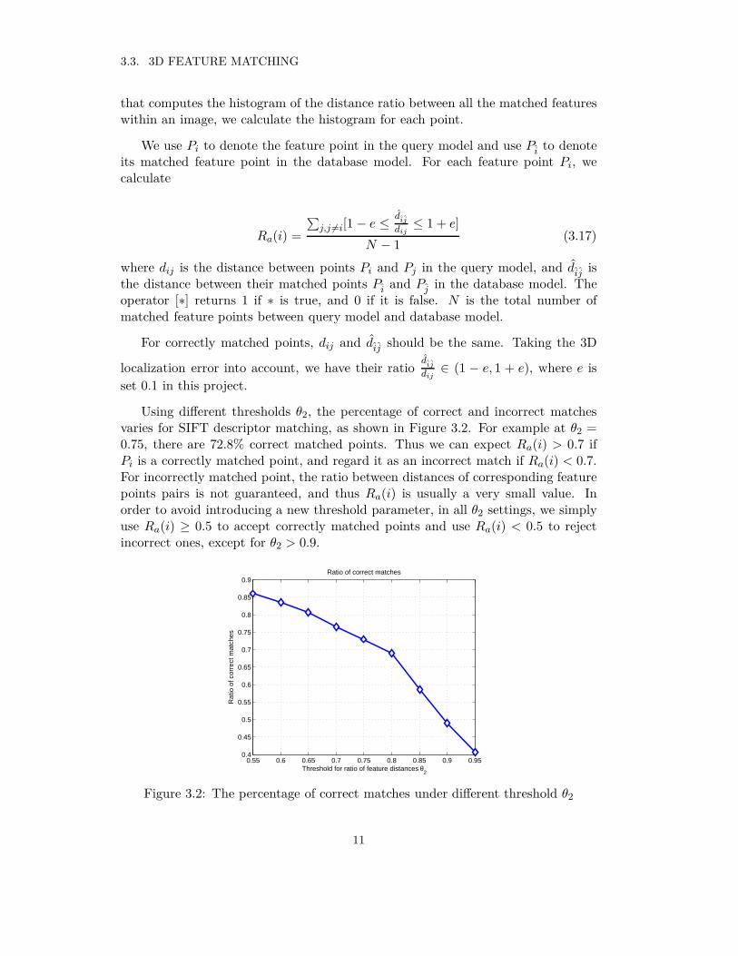
that computes the histogram of the distance ratio between all the matched featureswithin an image, we calculate the histogram for each point.
We use Pi to denote the feature point in the query model and use Pi to denoteits matched feature point in the database model. For each feature point Pi, wecalculate
Ra(i) =
∑
j,j 6=i[1 − e ≤d
ij
dij≤ 1 + e]
N − 1(3.17)
where dij is the distance between points Pi and Pj in the query model, and dij isthe distance between their matched points Pi and Pj in the database model. Theoperator [∗] returns 1 if ∗ is true, and 0 if it is false. N is the total number ofmatched feature points between query model and database model.
For correctly matched points, dij and dij should be the same. Taking the 3D
localization error into account, we have their ratiod
ij
dij∈ (1 − e, 1 + e), where e is
set 0.1 in this project.
Using different thresholds θ2, the percentage of correct and incorrect matchesvaries for SIFT descriptor matching, as shown in Figure 3.2. For example at θ2 =0.75, there are 72.8% correct matched points. Thus we can expect Ra(i) > 0.7 ifPi is a correctly matched point, and regard it as an incorrect match if Ra(i) < 0.7.For incorrectly matched point, the ratio between distances of corresponding featurepoints pairs is not guaranteed, and thus Ra(i) is usually a very small value. Inorder to avoid introducing a new threshold parameter, in all θ2 settings, we simplyuse Ra(i) ≥ 0.5 to accept correctly matched points and use Ra(i) < 0.5 to rejectincorrect ones, except for θ2 > 0.9.
0.55 0.6 0.65 0.7 0.75 0.8 0.85 0.9 0.950.4
0.45
0.5
0.55
0.6
0.65
0.7
0.75
0.8
0.85
0.9
Threshold for ratio of feature distances θ2
Ratio of correct matches
Rat
io o
f cor
rect
mat
ches
Figure 3.2: The percentage of correct matches under different threshold θ2
11

CHAPTER 3. 3D VISUAL SEARCH
This distance verification between feature points has the following advantages:
1. False positive ratio can be reduced.
2. Be able to distinguish between objects with the same 2D local image features,but having different 3D shapes and volumes, such as real object and photosof the real object, or real object and its scaled models.
3.4 Construction of Planar Models
For recognition of 3D objects, we want to pack the feature points in a way thatthose points together represent some geometric information. The simplest way topack the feature points is to find point pairs, where the 3D distance between thepair of points is used as 3D geometric information. However these methods arefragile because if one of these points fails to find its match in the database model,such a 3D geometric constraint fails to work.
However, some 3D objects, such as buildings, can be well approximated byplanes. It is observed that a considerable number of keypoints for buildings lie onthese planes, such as keypoints on windows, on walls and on roofs. Thus it is anatural way to model such objects using planes. By describing feature points thatlie on planes, and by comparing the angles between the surface normals of the planesthat they belong to, we will be able to distinguish between a true 3D object and aphoto of it.
3.4.1 Fitting of 3D Points
To fit 3D points in a plane, we use the least square method. Suppose wehave N points in 3D space with coordinates P1(X1, Y1, Z1), · · · , Pi(Xi, Yi, Zi), · · · ,PN (XN , YN , ZN ), that lie on a plane with some errors. The plane in 3D spacesatisfies the following plane equation
Z = aX + bY + c. (3.18)
For each point Pi, we can write its coordinates in the form of Eq. (3.18) witha residual error ξi. We want to find the plane parameters (a, b, c) such that theresidual errors are minimized. The linear equations of the N points are given inmatrix form as
12
3.4. CONSTRUCTION OF PLANAR MODELS
Z1
Z2
Z3
...Zi
...ZN
=
X1 Y1 1X2 Y2 1X3 Y3 1...
......
Xi Yi 1...
......
XN YN 1
abc
+
ξ1
ξ2
ξ3
...ξi
...ξN
(3.19)
We rewrite Eq.(3.19) in compact notation
~Z = M ~A + ~Ξ, (3.20)
then the least square solution to the problem is
M t ~Z = (M tM) ~A (3.21)
Solving for ~A we have~A′ = (M tM)−1M t ~Z (3.22)
The residual error of the planar model with plane parameters A is
~Ξ = ~Z − M ~A′ (3.23)
We define the plane fitting error as the mean square of residual errors.
ξ2 =
∑
i ξ2i
N(3.24)
When the plane fitting error ξ2 ≤ γ, where γ is a threshold, these N pointscan be considered to be fitted well by the plane as defined by the predicted planeparameters. Otherwise, these N points are not modeled as a plane.
3.4.2 Planar Model
Given the coordinates of all the feature points in 3D space, we need an algorithmto find the primary planes that fit these points. The output of this algorithm areplane equation parameters for each plane and subsets of feature points that lie onthat plane.
We want to design an algorithm which is towards the following goals:
13

CHAPTER 3. 3D VISUAL SEARCH
1. The algorithm should be able to detect the big planes that truly exist onthe building, such as walls and roofs, and try to find small planes as well aspossible.
2. Each detected plane should include as many feature points that truly lie onthat plane as possible.
3. The output of the algorithm should include as few mis-fitted points as possible.
With the above goals in mind, we design the planar model construction algo-rithm as follows.
Algorithm 1: Construct planar model
We denote the set of all feature points on the object as Λ, the number of pointsin Λ as NΛ, and the set of points that have NOT been confirmed to fit in any planeas Ω, the number of points in Ω as NΩ. We use the set Θ to denote the points inthe current fitting plane.
We denote the symbol ℘P as the set of neighboring points of point P , with adistance smaller than d. And the number of points in this neighboring set is N℘P .
Initialize algorithm: Ω = Λwhile Ω 6= ø do
for ∀Pi ∈ Ω doif N℘P ≥ 10 then
Initialize the fitting: ℘P → fZ = aX + bY + c, ξ2, Θ 1
if ξ2 ≤ γ then1. Update plane: fZ = aX + bY + c, ξ2, Θ →
f ′Z = a′X + b′Y + c′, ξ2′, Θ′ 2
2. Ω = Ω − Θ′
end ifend if
end forend while
1. Use the fitting algorithm described in Section 3.4.1, where ξ2 is the average fitting error, and
Θ is the set of points been fitted in the plane.
2. Use Algorithm 2: Update plane.
14

3.4. CONSTRUCTION OF PLANAR MODELS
Algorithm 2: Update plane
In order to fit more points in the plane and to update the plane parameters,we use the following algorithm. We denote the set of points that are already fit-ted in plane f as Φ, and the set of candidate points that are waiting to be fitted as Ψ.
Intialize: Ψ = Ω − Φwhile Ψ 6= ø do
1. xc =
∑
i∈Φxi
NΦ, yc =
∑
i∈Φyi
NΦ, zc =
∑
i∈Φzi
NΦ
2. i = argmini∈Ψ
‖(xi, yi, zi) − (xc, yc, zc)‖2
3. Φ′
= Φ + Pi
4. Φ′
→ f ′Z = a′X + b′Y + c′, ξ2′, Φ
′1
if ξ2′< γ then
Φ = Φ + Pi
Ψ = Ψ − Pi
goto 1else
Ψ = Ψ − Pi
goto 2end if
end while
3.4.3 Matching of Planar Model
For a plane with plane equation Z = aX + bY + c, its surface normal is
~n = (nx, ny, nz) =(a, b, −1)
‖a, b, −1‖2
(3.25)
The surface normal is stored for each plane, together with the SIFT descriptorsof the feature points lying on that plane. We do not store the coordinates of thefeature points in planar model. The plane will be stored like this:
1. Use the fitting algorithm described in Section 3.4.1.
15
CHAPTER 3. 3D VISUAL SEARCH
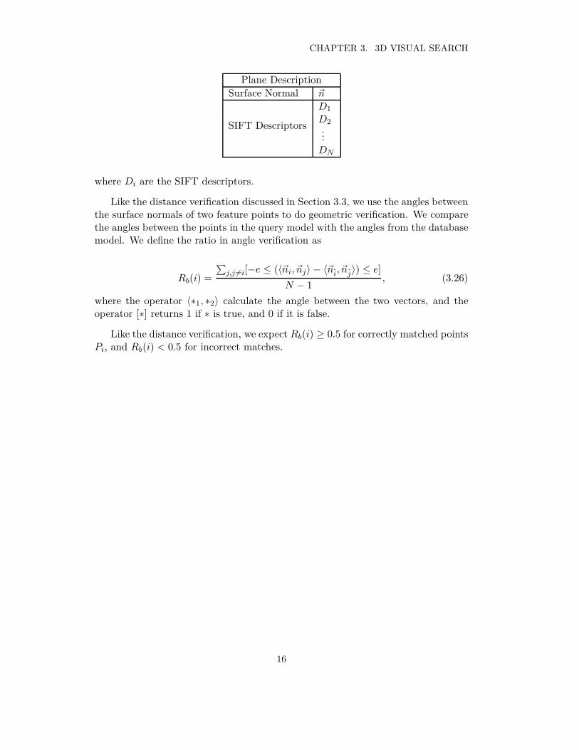
Plane Description
Surface Normal ~n
SIFT Descriptors
D1
D2
...DN
where Di are the SIFT descriptors.
Like the distance verification discussed in Section 3.3, we use the angles betweenthe surface normals of two feature points to do geometric verification. We comparethe angles between the points in the query model with the angles from the databasemodel. We define the ratio in angle verification as
Rb(i) =
∑
j,j 6=i[−e ≤ (〈~ni, ~nj〉 − 〈~ni, ~nj〉) ≤ e]
N − 1, (3.26)
where the operator 〈∗1, ∗2〉 calculate the angle between the two vectors, and theoperator [∗] returns 1 if ∗ is true, and 0 if it is false.
Like the distance verification, we expect Rb(i) ≥ 0.5 for correctly matched pointsPi, and Rb(i) < 0.5 for incorrect matches.
16
Chapter 4
Compression of 3D Features
Using 8 bits to store each dimension of the SIFT descriptor will result in evenlarger data size than the compressed picture using JPEG. To store the 3D infor-mation such as coordinates and surface normal using the floating-point data typewill consume even more bits. In this chapter we discuss how to compress the 3Dfeatures. CHoG, a recently proposed local image feature descriptor, is shown tohave low bitrate while maintaining satisfactory recognition rates [2]. Observingthat there exist considerable similarities among the quantized CHoG descriptorswithin an image, we try to code the differences between these descriptors in orderto make the bitrate even lower.
4.1 Compressed Histogram of Gradients
Many works have been done to decrease the data size of SIFT features. Unlikemethods which compress the SIFT descriptors directly, CHoG modifies the descrip-tor structure with compression in mind. The reduction of bitrate achieved by CHoGis mainly due to the compactly designed spatial binning schemes, gradient histogrambinning schemes and type coding of the gradient histograms.
CHoG first designs a compact spatial binning scheme to reduce the number ofspatial bins of each descriptor. Unlike the square 4 × 4 grid with 16 cells used bySIFT and SURF descriptors, CHoG uses log-polar configurations as shown in [22].Each spatial bin is weighted by overlapping 2-dimensional Gaussian functions. Itdesigns the DAISY configuration with K = 9, 13, 17 spatial bins. It is shownthat the DAISY-9 configuration matches the performance of the 4 × 4 square-gridconfiguration, and DAISY-13 is discriminative enough for feature point matching.
CHoG designs its bin configuration to have a bin at the origin in order to capturethe central peak of the gradient distribution. Observing that the joint distribution
17
CHAPTER 4. COMPRESSION OF 3D FEATURES
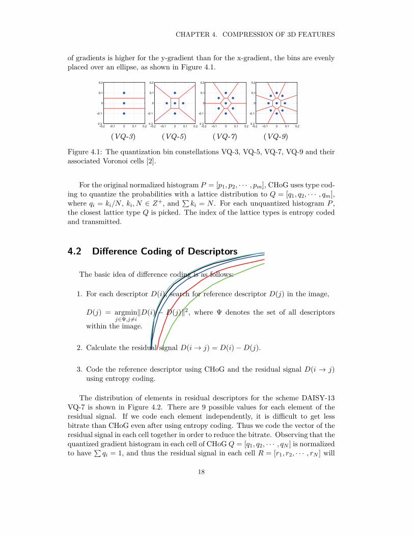
of gradients is higher for the y-gradient than for the x-gradient, the bins are evenlyplaced over an ellipse, as shown in Figure 4.1.
Figure 4.1: The quantization bin constellations VQ-3, VQ-5, VQ-7, VQ-9 and theirassociated Voronoi cells [2].
For the original normalized histogram P = [p1, p2, · · · , pm], CHoG uses type cod-ing to quantize the probabilities with a lattice distribution to Q = [q1, q2, · · · , qm],where qi = ki/N , ki, N ∈ Z+, and
∑
ki = N . For each unquantized histogram P ,the closest lattice type Q is picked. The index of the lattice types is entropy codedand transmitted.
4.2 Difference Coding of Descriptors
The basic idea of difference coding is as follows:
1. For each descriptor D(i), search for reference descriptor D(j) in the image,
D(j) = argminj∈Ψ,j 6=i
‖D(i) − D(j)‖2, where Ψ denotes the set of all descriptors
within the image.
2. Calculate the residual signal D(i → j) = D(i) − D(j).
3. Code the reference descriptor using CHoG and the residual signal D(i → j)using entropy coding.
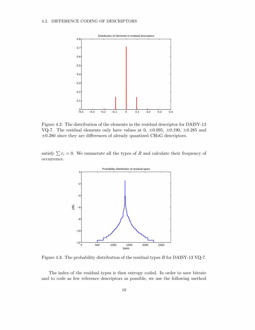
The distribution of elements in residual descriptors for the scheme DAISY-13VQ-7 is shown in Figure 4.2. There are 9 possible values for each element of theresidual signal. If we code each element independently, it is difficult to get lessbitrate than CHoG even after using entropy coding. Thus we code the vector of theresidual signal in each cell together in order to reduce the bitrate. Observing that thequantized gradient histogram in each cell of CHoG Q = [q1, q2, · · · , qN ] is normalizedto have
∑
qi = 1, and thus the residual signal in each cell R = [r1, r2, · · · , rN ] will
18
4.2. DIFFERENCE CODING OF DESCRIPTORS
−0.4 −0.3 −0.2 −0.1 0 0.1 0.2 0.3 0.40
0.1
0.2
0.3
0.4
0.5
0.6
0.7
0.8Distribution of elements in residual descriptors
Figure 4.2: The distribution of the elements in the residual descriptor for DAISY-13VQ-7. The residual elements only have values at 0, ±0.095, ±0.190, ±0.285 and±0.380 since they are differences of already quantized CHoG descriptors.
satisfy∑
ri = 0. We enumerate all the types of R and calculate their frequency ofoccurrence.
0 500 1000 1500 2000 2500−12
−10
−8
−6
−4
−2
0Probability distribution of residual types
types
(dB
)
Figure 4.3: The probability distribution of the residual types R for DAISY-13 VQ-7.
The index of the residual types is then entropy coded. In order to save bitrateand to code as few reference descriptors as possible, we use the following method
19
CHAPTER 4. COMPRESSION OF 3D FEATURES
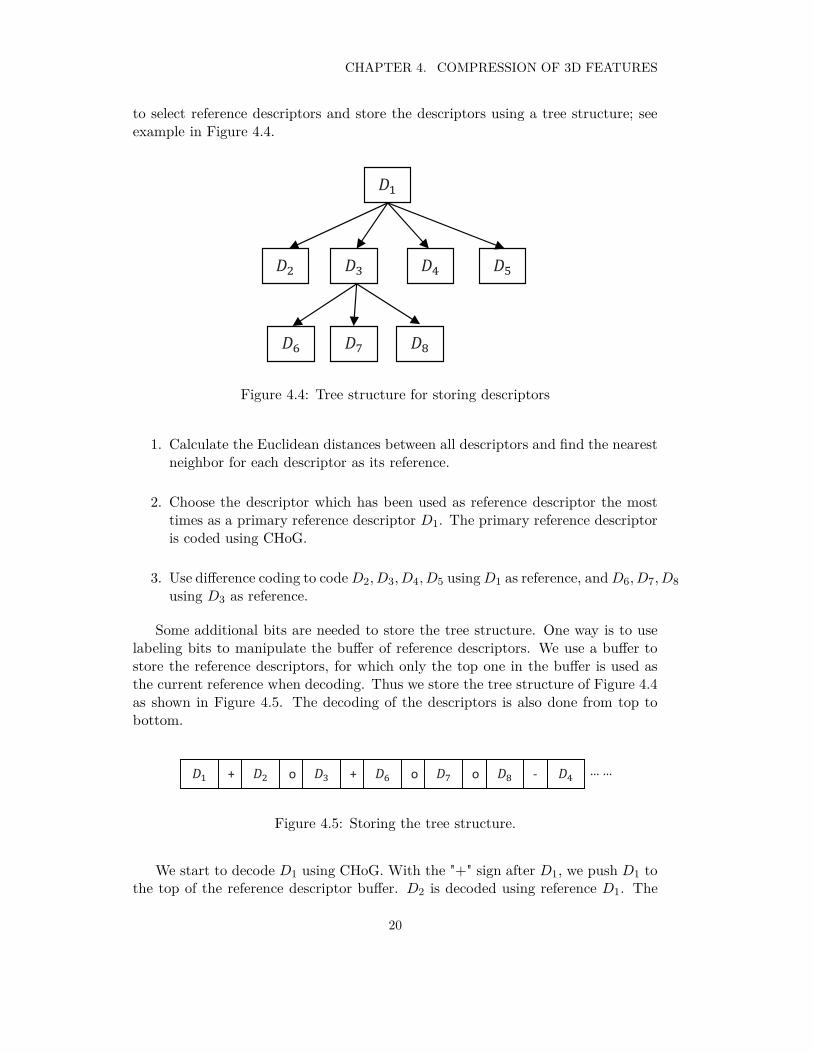
to select reference descriptors and store the descriptors using a tree structure; seeexample in Figure 4.4.
! " #
$
% & '
(
Figure 4.4: Tree structure for storing descriptors
1. Calculate the Euclidean distances between all descriptors and find the nearestneighbor for each descriptor as its reference.
2. Choose the descriptor which has been used as reference descriptor the mosttimes as a primary reference descriptor D1. The primary reference descriptoris coded using CHoG.
3. Use difference coding to code D2, D3, D4, D5 using D1 as reference, and D6, D7, D8
using D3 as reference.
Some additional bits are needed to store the tree structure. One way is to uselabeling bits to manipulate the buffer of reference descriptors. We use a buffer tostore the reference descriptors, for which only the top one in the buffer is used asthe current reference when decoding. Thus we store the tree structure of Figure 4.4as shown in Figure 4.5. The decoding of the descriptors is also done from top tobottom.
! " # $% & '
)
*… … + o + o o !
Figure 4.5: Storing the tree structure.
We start to decode D1 using CHoG. With the "+" sign after D1, we push D1 tothe top of the reference descriptor buffer. D2 is decoded using reference D1. The
20

4.2. DIFFERENCE CODING OF DESCRIPTORS
"o" after D2 means no manipulation of the buffer. Thus, D3 is also decoded usingD1 as reference. D3 is pushed to the top of the buffer with the "+" after it andD6, D7 and D8 are all decoded using reference D3. The sign "-" after D8 meanspushing out the top descriptor, which is currently D3. After pushing out D3, D1
comes to the top of the buffer, and D4 and D5 are decoded using reference D1. Theprocedure continues until the whole tree is decoded.
21

Chapter 5
Experimental Results
5.1 Experimental Setup
We use the dataset of the Visual Geometry Group from Oxford Universy [23].This dataset consists of five groups of multiview images taken from five buildings onthe campus. Each group consists of 3-5 multiview images, with a camera projectionmatrix for each image. We use adjacent views as stereo pairs for 3D reconstruction.We use the implementation from David Lowe [24] to compute the SIFT features ofan image. The implementation of computing CHoG features is obtained from VijayChandrasekhar [25].
For each group of multiview images in the dataset, we divide them into twostereo pairs. We use one of them as query data, and the other pair as the databasedata. For those groups containing only three images, we use view 1 and view 2 aspair 1, view 2 and view 3 as pair 2. For the groups containing more than threeimages, we use adjacent two views as a stereo pair. The database data consistsof five stereo pairs of images from five different buildings. During the recognitiontest, the 3D features extracted from the query data are compared with the featuresextracted from the five database data. In the experiments using CHoG, we use adatabase of Merton College I, II and III.
Since the software used for detecting CHoG features does not implement subpixelrefinement in feature point localization, the 3D locations calculated from matchedpoints contain more errors compared with that using SIFT features. More impor-tantly, CHoG uses an extra threshold to limit the number of features points thatit detects, and thus results in sparser 3D points, which is not favorable for planefitting. The experiment on planar model construction using CHoG is not very suc-cessful, resulting in very sparse points on one or two planes. For these reasons, wetest only the recognition rate of CHoG features using distance verifications. Theplanar model method can be tested if the CHoG implementation can be modified
23
CHAPTER 5. EXPERIMENTAL RESULTS
in the future.
5.2 Stereo Images Synthesis
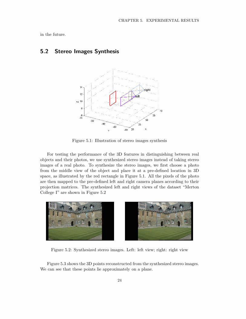
Figure 5.1: Illustration of stereo images synthesis
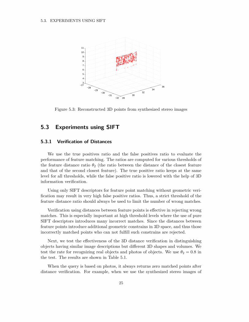
For testing the performance of the 3D features in distinguishing between realobjects and their photos, we use synthesized stereo images instead of taking stereoimages of a real photo. To synthesize the stereo images, we first choose a photofrom the middle view of the object and place it at a pre-defined location in 3Dspace, as illustrated by the red rectangle in Figure 5.1. All the pixels of the photoare then mapped to the pre-defined left and right camera planes according to theirprojection matrices. The synthesized left and right views of the dataset “MertonCollege I” are shown in Figure 5.2
Figure 5.2: Synthesized stereo images. Left: left view; right: right view
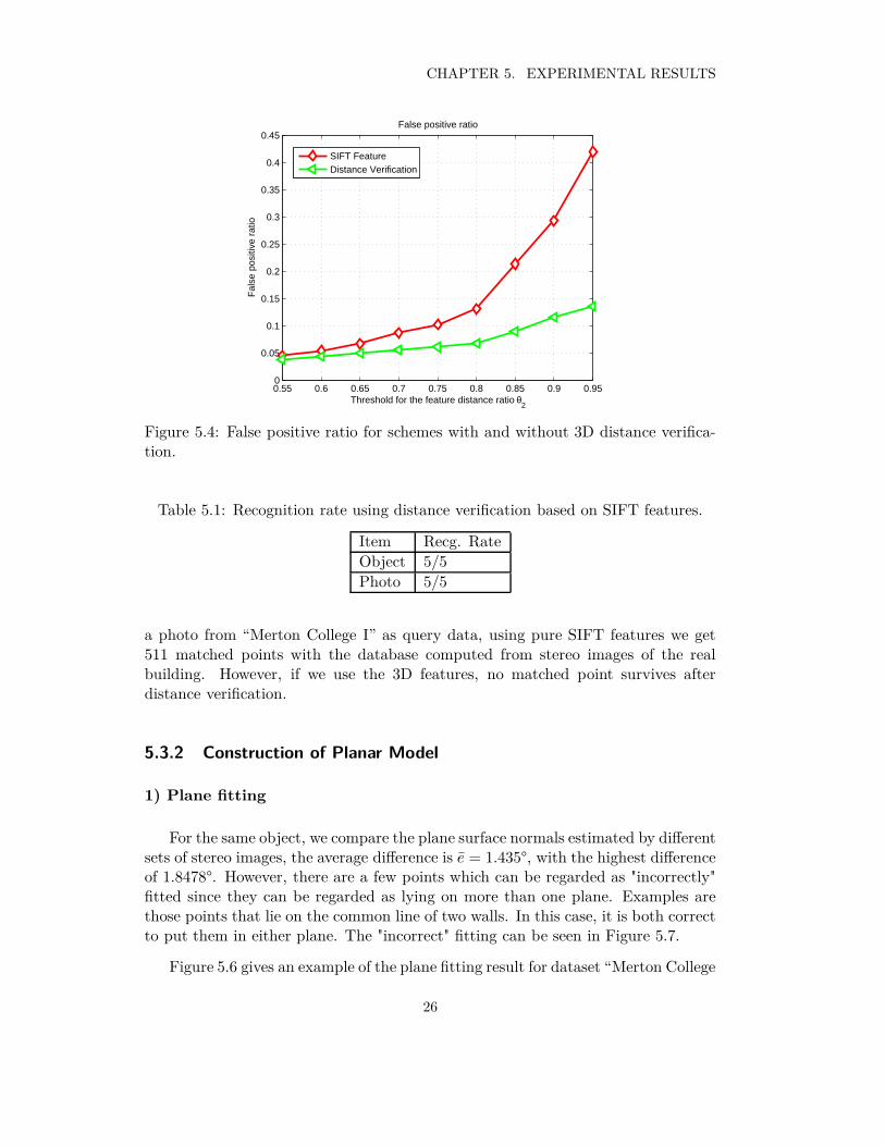
Figure 5.3 shows the 3D points reconstructed from the synthesized stereo images.We can see that these points lie approximately on a plane.
24
5.3. EXPERIMENTS USING SIFT
2830
3234
36
−32−31
−30−29
−28−27
3
4
5
6
7
8
9
10
11
Figure 5.3: Reconstructed 3D points from synthesized stereo images
5.3 Experiments using SIFT
5.3.1 Verification of Distances
We use the true positives ratio and the false positives ratio to evaluate theperformance of feature matching. The ratios are computed for various thresholds ofthe feature distance ratio θ2 (the ratio between the distance of the closest featureand that of the second closest feature). The true positive ratio keeps at the samelevel for all thresholds, while the false positive ratio is lowered with the help of 3Dinformation verification.
Using only SIFT descriptors for feature point matching without geometric veri-fication may result in very high false positive ratios. Thus, a strict threshold of thefeature distance ratio should always be used to limit the number of wrong matches.
Verification using distances between feature points is effective in rejecting wrongmatches. This is especially important at high threshold levels where the use of pureSIFT descriptors introduces many incorrect matches. Since the distances betweenfeature points introduce additional geometric constrains in 3D space, and thus thoseincorrectly matched points who can not fulfill such constrains are rejected.
Next, we test the effectiveness of the 3D distance verification in distinguishingobjects having similar image descriptions but different 3D shapes and volumes. Wetest the rate for recognizing real objects and photos of objects. We use θ2 = 0.8 inthe test. The results are shown in Table 5.1.
When the query is based on photos, it always returns zero matched points afterdistance verification. For example, when we use the synthesized stereo images of
25
CHAPTER 5. EXPERIMENTAL RESULTS
0.55 0.6 0.65 0.7 0.75 0.8 0.85 0.9 0.950
0.05
0.1
0.15
0.2
0.25
0.3
0.35
0.4
0.45
Threshold for the feature distance ratio θ2
Fal
se p
ositi
ve r
atio
False positive ratio
SIFT FeatureDistance Verification
Figure 5.4: False positive ratio for schemes with and without 3D distance verifica-tion.
Table 5.1: Recognition rate using distance verification based on SIFT features.
Item Recg. Rate
Object 5/5
Photo 5/5
a photo from “Merton College I” as query data, using pure SIFT features we get511 matched points with the database computed from stereo images of the realbuilding. However, if we use the 3D features, no matched point survives afterdistance verification.
5.3.2 Construction of Planar Model
1) Plane fitting
For the same object, we compare the plane surface normals estimated by differentsets of stereo images, the average difference is e = 1.435°, with the highest differenceof 1.8478°. However, there are a few points which can be regarded as "incorrectly"fitted since they can be regarded as lying on more than one plane. Examples arethose points that lie on the common line of two walls. In this case, it is both correctto put them in either plane. The "incorrect" fitting can be seen in Figure 5.7.
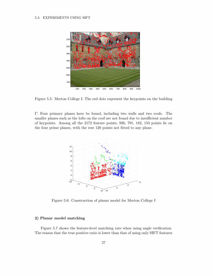
Figure 5.6 gives an example of the plane fitting result for dataset “Merton College
26
5.3. EXPERIMENTS USING SIFT
100 200 300 400 500 600 700 800 900 1000
100
200
300
400
500
600
700
Figure 5.5: Merton College I. The red dots represent the keypoints on the building
I”. Four primary planes have be found, including two walls and two roofs. Thesmaller planes such as the lofts on the roof are not found due to insufficient numberof keypoints. Among all the 2172 feature points, 926, 791, 182, 153 points lie onthe four prime planes, with the rest 120 points not fitted to any plane.
−50
510
−10−5
05
10
−2
0
2
4
6
8
10
12
Figure 5.6: Construction of planar model for Merton College I
2) Planar model matching
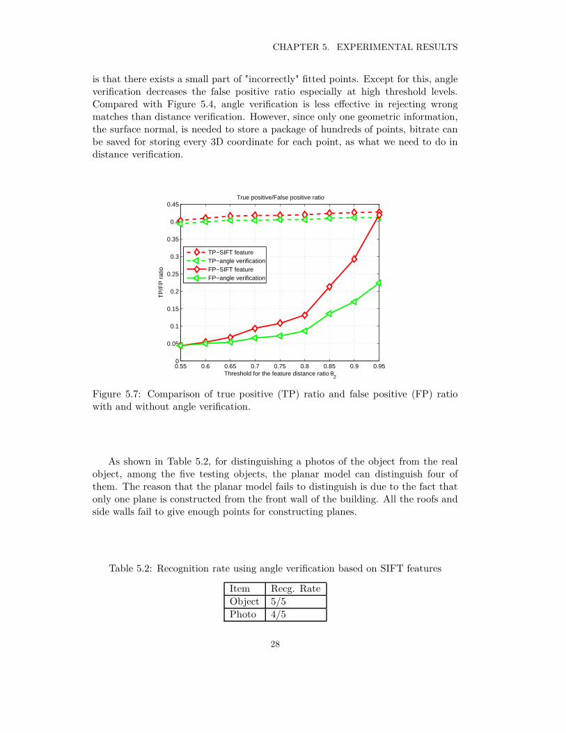
Figure 5.7 shows the feature-level matching rate when using angle verification.The reason that the true positive ratio is lower than that of using only SIFT features
27
CHAPTER 5. EXPERIMENTAL RESULTS
is that there exists a small part of "incorrectly" fitted points. Except for this, angleverification decreases the false positive ratio especially at high threshold levels.Compared with Figure 5.4, angle verification is less effective in rejecting wrongmatches than distance verification. However, since only one geometric information,the surface normal, is needed to store a package of hundreds of points, bitrate canbe saved for storing every 3D coordinate for each point, as what we need to do indistance verification.
0.55 0.6 0.65 0.7 0.75 0.8 0.85 0.9 0.950
0.05
0.1
0.15
0.2
0.25
0.3
0.35
0.4
0.45
Threshold for the feature distance ratio θ2
TP
/FP
rat
io
True positive/False positive ratio
TP−SIFT featureTP−angle verificationFP−SIFT featureFP−angle verification
Figure 5.7: Comparison of true positive (TP) ratio and false positive (FP) ratiowith and without angle verification.
As shown in Table 5.2, for distinguishing a photos of the object from the realobject, among the five testing objects, the planar model can distinguish four ofthem. The reason that the planar model fails to distinguish is due to the fact thatonly one plane is constructed from the front wall of the building. All the roofs andside walls fail to give enough points for constructing planes.
Table 5.2: Recognition rate using angle verification based on SIFT features
Item Recg. Rate
Object 5/5
Photo 4/5
28
5.4. EXPERIMENTS USING CHOG
Table 5.3: Bits per descriptor (bpd) for coding the differences between descriptorsfor 3D object recognition.
Binning Schemes CHoG (bpd) Residual (bpd)
DAISY-13 VQ-7 102.06 88.18
DAISY-13 VQ-5 61.35 57.13
DAISY-9 VQ-7 69.98 58.90
DAISY-9 VQ-5 41.11 29.33
Table 5.4: Bits per descriptor for coding the differences between descriptors for 2Dimage recognition.
Binning Schemes CHoG (bpd) Residual (bpd)
DAISY-13 VQ-7 102.06 84.71
DAISY-13 VQ-5 61.354 52.36
DAISY-9 VQ-7 69.98 53.72
DAISY-9 VQ-5 41.11 24.03
5.4 Experiments using CHoG
5.4.1 Discriptor Differences
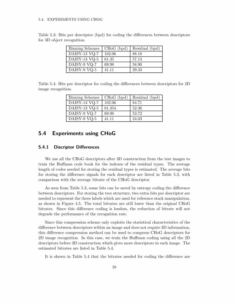
We use all the CHoG descriptors after 3D construction from the test images totrain the Huffman code book for the indexes of the residual types. The averagelength of codes needed for storing the residual types is estimated. The average bitsfor storing the difference signals for each descriptor are listed in Table 5.3, withcomparison with the average bitrate of the CHoG descriptor.
As seen from Table 5.3, some bits can be saved by entropy coding the differencebetween descriptors. For storing the tree structure, two extra bits per descriptor areneeded to represent the three labels which are used for reference stack manipulation,as shown in Figure 4.5. The total bitrates are still lower than the original CHoGbitrates. Since this difference coding is lossless, the reduction of bitrate will notdegrade the performance of the recognition rate.
Since this compression scheme only exploits the statistical characteristics of thedifference between descriptors within an image and does not require 3D information,this difference compression method can be used to compress CHoG descriptors for2D image recognition. In this case, we train the Huffman coding using all the 2Ddescriptors before 3D construction which gives more descriptors in each image. Theestimated bitrates are listed in Table 5.4.
It is shown in Table 5.4 that the bitrates needed for coding the difference are
29
CHAPTER 5. EXPERIMENTAL RESULTS
even lower for 2D image recognition. The reason is that for 3D recognition manyfeatures points are filtered out during 3D reconstruction due to mismatch. Withmore descriptors in an image, it is more likely that the descriptors find their nearestneighbor with smaller energy in the residual signal. Although DAISY-13 VQ-5 (65dimensions) has more dimensions than DAISY-9 VQ-7 (63 dimensions), DAISY-9VQ-7 needs more bits for storing the residual. This is because with longer vector,VQ-7 has a much larger code space than VQ-5 and thus, is less efficient in entropycoding.
5.4.2 Recognition Rate
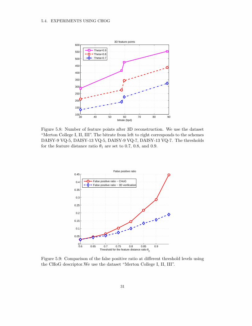
We use the quantized CHoG features for stereo matching. With the decreasein dimensionality for the CHoG descriptor, the ability of the CHoG descriptor todiscriminate decreases dramatically, and thus, the performance of stereo matchingdecreases. The number of feature points after 3D reconstruction is shown in Figure5.8. The bitrate is estimated according to Table 5.3.
From Figure 5.8 it is observed that schemes using VQ-7 always surpass theschemes using VQ-5 in the performance of stereo matching. Comparing the num-ber of 3D feature points using DAISY-13 VQ-5 and DAISY-9 VQ-7 we can seethat, although DAISY-13 VQ-5 has more dimensions in descriptors (65 dimensions),DAISY-9 VQ-7 (63 dimensions) gives more correct stereo matches which results inmore constructed 3D points.
Like the method used in Section 5.3.1, we do distance verification after thematching of the CHoG descriptor. We quantize the 3D coordinates using 8 bits foreach dimension. Still, the true positive ratio is the same with and without distanceverification, as for the SIFT descriptor. The false positive ratio is shown in Figure5.9.
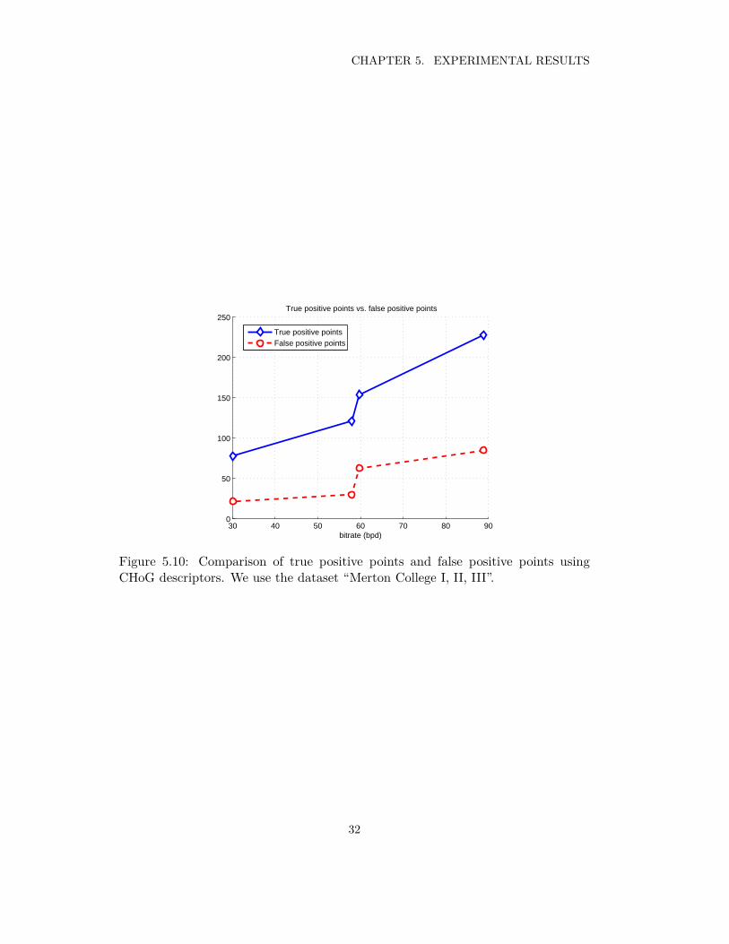
Since the number of 3D feature points varies at different bitrates, it is not a goodway to compare their true positive ratio or false positive ratio at different bitrates.As all the 3D features are extracted from the same stereo images, we compare theirfinal number of points of true matches and false matches. The comparison is givenin Figure 5.10. There is a jump from DAISY-13 VQ-5 to DAISY-9 VQ-7 for bothtrue positive and false positive numbers. The false positive numbers change verylittle as long as the same VQ schme is used, but the true positive number increasesfrom DAISY-9 to DAISY-13, mainly because of the increase in 3D feature points,as shown in Figure 5.8.
30
5.4. EXPERIMENTS USING CHOG
30 40 50 60 70 80 90100
150
200
250
300
350
400
450
500
550
600
bitrate (bpd)
3D feature points
Theta=0.9Theta=0.8Theta=0.7
Figure 5.8: Number of feature points after 3D reconstruction. We use the dataset“Merton College I, II, III”. The bitrate from left to right corresponds to the schemesDAISY-9 VQ-5, DAISY-13 VQ-5, DAISY-9 VQ-7, DAISY-13 VQ-7. The thresholdsfor the feature distance ratio θ1 are set to 0.7, 0.8, and 0.9.
0.6 0.65 0.7 0.75 0.8 0.85 0.90
0.05
0.1
0.15
0.2
0.25
0.3
0.35
0.4
0.45
Threshold for the feature distance ratio θ2
False positive ratio
False positive ratio − CHoGFalse positive ratio − 3D verification
Figure 5.9: Comparison of the false positive ratio at different threshold levels usingthe CHoG descriptor.We use the dataset “Merton College I, II, III”.
31
CHAPTER 5. EXPERIMENTAL RESULTS
30 40 50 60 70 80 900
50
100
150
200
250
bitrate (bpd)
True positive points vs. false positive points
True positive pointsFalse positive points
Figure 5.10: Comparison of true positive points and false positive points usingCHoG descriptors. We use the dataset “Merton College I, II, III”.
32
Chapter 6
Conclusions
In this project, we designed and tested methods for mobile 3D visual search.We use stereo images to obtain the 3D locations of feature points and to fit these3D points to planes to get their surface normals. We use distances between featurepoints and angles between surfaces as 3D geometric constrains when recognizing 3Dobjects. The results show that distances between feature points can distinguish ob-jects having similar image appearance but different 3D shapes, such as real objects,photos of objects and small model of objects. Angles between surfaces are able todistinguish photos of objects from real objects in most cases. Besides, both meth-ods help to reduce incorrect matches by introducing additional geometric constrains.The tests using CHoG descriptors show that DAISY-13 VQ-7 is satisfactory in 3Dreconstruction and recognition. All other schemes are not discriminative enough forstereo matching and thus have poor performance in 3D reconstruction. The resultsof compressing CHoG descriptors show that by coding the difference between quan-tized CHoG descriptors in an image, the bitrate can be reduced by 10% - 35% fordifferent binning schemes.
Since the CHoG descriptors we use in this project are already quantized becauseof the used CHoG implementation, a future direction may be modifying the imple-mentation of CHoG, such that it gives the original feature points and descriptorsto support subpixel localization. We use the descriptor differences for compression.Since most of the elements in the residual signals are zeros, it is possible to usesome sparse representation method to represent and code the residual. Compressedsensing techniques may be used in the future. The distances between feature pointsare shown to be effective for both distinguishing objects and rejecting incorrectmatches. Since the 3D location of each feature point has to be transmitted, furtherwork can be done to represent the 3D locations using as few bits as possible.
33

Bibliography
[1] D. Lowe, “Distinctive image features from scale-invariant keypoints,” Interna-
tional Journal of Computer Vision, vol. 60(2), pp. 91–110, 2004.
[2] B. Girod, V. Chandrasekhar, D. M. Chen, N. M. Cheung, R. Grzeszczuk,Y. Reznik, G. Takacs, S. S. Tsai, and R. Vedantham, “Compressed histogramof gradients: A low-bitrate descriptor,” International Journal of Computer
Vision, vol. 96(3), pp. 384–399, 2012.
[3] H. Baya, A. Essa, T. Tuytelaarsb, and L. V. Goola, “Speeded-up robust fea-tures (SURF),” Computer Vision and Image Understanding, vol. 110(3), pp.346–359, 2008.
[4] H. Li and M. Flierl, “SIFT-based multi-view cooperative tracking for soccervideo,” in Proc. of the IEEE International Conference on Acoustics, Speech,
and Signal Processing, Mar. 2012.
[5] Y. Furukawa and J. Ponce, “Accurate, dense, and robust multi-view stereop-sis,” IEEE Conference on Computer Vision and Pattern Recognition, pp. 1–8,2007.
[6] D. Lowe, “Object recognition from local scale-invariant features,” International
Conference on Computer Vision, Corfu, Greece, pp. 1150–1157, 1999.
[7] D. Lowe, “Local feature view clustering for 3d object recognition,” IEEE
Conference on Computer Vision and Pattern Recognition, Kauai, Hawaii, pp.682–688, 2001.
[8] C. Yeo, P. Ahammad, and K. Ramchandran, “Rate-efficient visual correspon-dences using random projections,” IEEE International Conference on Image
Processing, San Diego, California, 2008.
[9] A. Torralba, R. Fergus, and Y. Weiss, “Small codes and large image databasesfor recognition,” IEEE Conference on Computer Vision and Pattern Recogni-
tion, 2008.
[10] V. Chandrasekhar, G. Takacs, D. M. Chen, S. S. Tsai, and B. Girod, “Trans-form coding of feature descriptors,” Visual Communications and Image Pro-
cessing Conference, 2009.
35
BIBLIOGRAPHY
[11] D. Nistér and H. Stewénius, “Scalable recognition with a vocabulary tree,” In
Proc. of the IEEE Conference on Computer Vision and Pattern Recognition,
New York, USA, 2006.
[12] V. Chandrasekhar, M. Maker, G. Takacs, D. M. Chen, S. S. Tsai, N. M. Che-ung, R. Grzeszczuk, Y. Reznik, and B. Girod, “Survey of SIFT compressionschemes,” In Proc. of the IEEE International Mobile Multimedia Workshop,
Istanbul, Turkey, 2010.
[13] V. Chandrasekhar, D. M. Chen, A. Lin, G. Takacs, S. S. Tsai, N. M. Cheung,Y. Reznik, R. Grzeszczuk, and B. Girod, “Comparison of local feature de-scriptors for mobile visual search,” IEEE International Conference on Image
Processing, Hong Kong, 2010.
[14] B. Girod, V. Chandrasekhar, D. M. Chen, N. M. Cheung, R. Grzeszczuk,Y. Reznik, G. Takacs, S. S. Tsai, and R. Vedantham, “Mobile visual search,”Signal Processing Magazine, IEEE, vol. 28(4), pp. 61, 2011.
[15] M. A. Fischler and R. C. Bolles, “Random sample consensus: a paradigm formodel fitting with applications to image analysis and automated cartography,”ACM Communications Magazine, vol. 24(6), pp. 381–395, 1981.
[16] A. Johnson, “Spin-images: A representation for 3-d surface matching,” PhD
thesis, Robotics Institute, Carnegie Mellon University, Pittsburgh, PA, 1997.
[17] L. J. Skelly and S. Sclaroff, “Improved feature descriptors for 3-d surfacematching,” Proc. of SPIE, vol. 6762, 2007.
[18] A. P. Ashbrook, R. B. Fisher, C. Robertson, , and N. Werghi, “Finding surfacecorrespondance for object recognition and registration using pairwise geometrichistograms,” European Conference on Computer Vision, vol. 1407, pp. 674–686, 1998.
[19] A. Makadia, A. I. Patterson, and K. Daniilidis, “Fully automatic registrationof 3d point clouds,” IEEE Computer Society Conference on Computer Vision
and Pattern Recognition, pp. 1297–1304, 2006.
[20] F. Rothganger, S. Lazebnik, C. Schmid, and J. Ponce, “3d object modelingand recognition using local affine-invariant image descriptors and multi-viewspatial constraints,” International Journal of Computer Vision, vol. 66(3), pp.231–259, 2006.
[21] S. Carlsson, “Geometric computing in image analysis and visualization,” Lec-
ture Notes, Numerical Analysis and Computing Science, KTH, Stockholm, Swe-
den, 2007.
[22] S. Winder, G. Hua, and M. Brown, “Picking the best daisy,” IEEE Conference
on Computer Vision and Pattern Recognition, pp. 178–185, 2009.
36

[23] Visual Geometry Group of Oxford University, Multiview dataset, http://
www.robots.ox.ac.uk/~vgg/data/data-mview.html, [Online; accessed May11, 2012].
[24] D. Lowe, Demo Software: SIFT Keypoint Detector, http://www.cs.ubc.ca/
~lowe/keypoints/, [Online; accessed Mar. 06, 2012].
[25] V. Chandrasekhar, CHoG binary, http://www.stanford.edu/~vijayc/
others.html, [Online; accessed May. 02, 2012].
37