mobile mapping by integrating structure from motion ... mapping by integrating structure from ......
TRANSCRIPT

JAYSON JAYESHKUMAR JARIWALA March, 2013
ITC SUPERVISOR IIRS SUPERVISORS
Dr. K. Khoshelham Er. Ashutosh Bhardwaj
Er. S. Raghavendra
Mobile Mapping by integrating Structure from Motion approach with Global Navigation Satellite System


Thesis submitted to the Faculty of Geo-information
Science and Earth Observation of the University of
Twente in partial fulfilment of the requirements for
the degree of Master of Science in Geo-information
Science and Earth Observation.
Specialization: Geoinformatics
THESIS ASSESSMENT BOARD: Chairperson : Prof. dr. ir. M.G. Vosselman
External Examiner : Dr. Kamal Jain (IIT, Roorkee)
ITC Supervisor : Dr. K. Khoshelham
IIRS Supervisor : Er. Ashutosh Bhardwaj
IIRS Supervisor : Er. S. Raghavendra
OBSERVERS:
ITC Observer : Dr. Nicholas Hamm
IIRS Observer : Dr. S. K. Srivastav
Mobile Mapping by integrating Structure from Motion approach with Global Navigation Satellite System
JAYSON JAYESHKUMAR JARIWALA
Enschede, the Netherlands [March, 2013]

DISCLAIMER This document describes work undertaken as part of a programme of study at the Faculty of
Geo-information Science and Earth Observation (ITC), University of Twente, The
Netherlands. All views and opinions expressed therein remain the sole responsibility of the
author, and do not necessarily represent those of the institute.

Dedicated to my parents.…


i
ABSTRACT
Over the past few years, there is an emerging growth in mobile mapping systems which can
effectively capture the geospatial data in an efficient way. A typical terrestrial mobile mapping
system consists of camera, laser scanners, GNSS (Global Navigation Satellite System) and INS
(Inertial Navigation System). Imagery data is captured by camera and the point clouds are
acquired by the laser scanners. GNSS and INS are used for measuring the positional and
orientation information of the mapping sensors respectively to achieve direct geo-referencing.
GNSS/INS system is very expensive which makes the overall mapping system very expensive.
An alternative to make this system is to use Structure from Motion Approach (SfM), to minimize
the relative cost of this system. SfM generates 3D point clouds of scene and estimate the
orientation parameter for mapping sensor by using imagery data. The major issue with SfM is that
it generates point clouds in arbitrary coordinate system with arbitrary scale.
In this research work, the feasibility of mapping by integration of the structure from motion
approach and GNSS was assessed to generate geo-referenced point clouds. In the first step,
sequences of images were captured by measuring the exposure station positions. Then feature
extractions and matching were done on the sequence of overlapping images. Bundle adjustment
was then applied on it to generate the 3D scene (point clouds) of rigid body and for estimation of
camera orientation parameters. The generated point clouds were in arbitrary coordinate system,
so tie points were selected to transform into mapping coordinate system. Space photo
intersection was applied on tie points with the use of exposure orientation parameters and
matched feature points in sequence of overlapping images to transform into world coordinate
system. Further, point-based similarity transformation was used to generate transformation
parameters from tie points. These transformation parameters were applied on whole generated
point cloud to transform it into world coordinate system with proper scale. Then the accuracy
assessments on point cloud were carried out using internal and external accuracy assessment.
Sometime the epipolar lines do not exactly cross at a fixed point in different overlapping images
due to which a distorted 3D scene (point clouds) was created. There was an error in the
estimation of orientation parameters due to no ground measurements were used in bundle
adjustment. Thus it was observed that the shape of the point cloud was concaved near start and
end edges of the scene. RMSE were 32.21 cm, 20.50 cm and 23.56 cm in easting, northing
(depth) and height respectively.
Keywords: Mobile Mapping, Terrestrial Photogrammetry, Structure from Motion, Global Navigation Satellite
System, Feature extraction, Feature matching, Space photo intersection, 3D similarity transformation.

ii
ACKNOWLEDGEMENTS
It is a great opportunity for me to get an admission in such a wonderful course of MSc, IIRS-ITC
JEP. I would like to express my gratitude to all the people who has supported me during my
entire MSc research work. It is little hard for me to list out all the names who had helped me to
make this achievements but I will try.
On the completion of my MSc thesis, I owe my deepest gratitude to my both IIRS supervisors
Er. Ashutosh Bhardwaj and Er. S. Raghavendra for their continuous support, guidance,
motivation and extraordinary scientific perception. Thank you sir, for your precious time, support
throughout my academics at IIRS. They helped me whenever I had approached them, even
during my hard time. Thank you again sir.
I would like to thank Dr. K. Khoshelham, my ITC supervisor, for his valuable guidance and
valuable suggestions at every stage of this research work. It is he, who had given such an
innovative and interesting research work and taught me vast knowledge of computer vision and
digital photogrammetry field.
I am grateful to Dr. Y.V.N. Krishna Murthy, the Director, IIRS and Dr. P.S. Roy, Former
Director, IIRS for providing excellent research environment and infrastructure to carry out this
research work. I would like to show my extreme gratitude to Mr. P.L.N. Raju, Group Head,
RSGG, IIRS for his constant support and providing critical inputs for making this MSc program
an invaluable experience. I would also like to acknowledge Dr. S. K. Srivastava, Head,
Geoinformatics Department, IIRS for taking care of our needs and giving their time to analyse
our progress. I would like to thank Ms. Shefali Agarwal, Head, PRSD, IIRS for providing me lab
facility in her division.
I am also honoured by receiving lectures from Prof. dr. ir. M.G. (George) Vosselman, Dr. ing. M.
Gerke and Dr. ir. S.J. Oude Elberink, ITC in the field 3D Geo-Information.
I express my hearty gratitude to Mr. Bashar Al-Sadik, Ph.D. student, ITC for his help and
support during my MSc research work.
Finally, deepest of gratitude to all my friends Chotu, Motu, Moti, Fatty, S.C., Sumu, Hongita,
Deepu, Psycho, Abdalla, Hemu, Mrinal, Shanky, Sai, Pajji, Bhavya garu, Prapti, Ravi, Chetan and
Anukesh. I will never forget the time we spent together: taking course, enjoying party, nice
excursion and travelling experience in Europe and INDIA. Thanks to my juniors Ankur, Mayank,
Shishant, Anant, Yeshu, Suman, Manisha, Ridhika, Binayak, and Jyostna for helping me
throughout my time at IIRS.
At last, I offer my greatest appreciation to my Mummy, Papa, Bhai Tayson, Vini, Keyur, Pri,
Dimps, Er. Jay, Dr. Vishal, Dr. Ankit and Master-Jariwala family for their infinite support.

iii
TABLE OF CONTENTS
List of Figures .......................................................................................................................V
List of Tables .................................................................................................................... VII
1. INTRODUCTION ........................................................................................................1
1.1. Background ................................................................................................................................ 1
1.1.1 Terrestrial Mobile Mapping ............................................................................................ 1
1.1.2. Global Navigation Satellite System (GNSS) ............................................................... 2
1.1.3. Structure from Motion Approach (SfM) ..................................................................... 3
1.2. Motivation and Problem Statement........................................................................................ 4
1.3. Research Identification ............................................................................................................. 5
1.3.1 Research Objectives ........................................................................................................ 5
1.3.2. Research Questions ........................................................................................................ 5
1.4. Thesis Structure ......................................................................................................................... 6
2. LITERATURE REVIEW AND THEORETICAL BACKGROUND ....................... 7
2.1. Camera Parameters ................................................................................................................... 8
2.1.1 Pinhole Model .................................................................................................................. 8
2.1.2. Intrinsic and Extrinsic Parameters ............................................................................... 9
2.1.3. Projection Matrix .......................................................................................................... 10
2.1.4. Epipolar Geometry ....................................................................................................... 10
2.2. Feature Extraction and Matching ......................................................................................... 13
2.3. Multiple view Geometry for SfM .......................................................................................... 17
3. MATERIALS AND METHODOLOGY ..................................................................... 21
3.1. Study Area and Data ............................................................................................................... 21
3.2. Tools Used ............................................................................................................................... 22
3.2.1. Hardware Tools ............................................................................................................ 22
3.2.2. Software Tools .............................................................................................................. 23
3.3. Methodology ............................................................................................................................ 24
3.3.1. Camera Calibration ....................................................................................................... 26
3.3.2. Planning for Data Acquisition .................................................................................... 26
3.3.3. Features Extraction ...................................................................................................... 28
3.3.4. Bundler ........................................................................................................................... 28
3.3.5. PMVS (Patch Based Multi-view Stereo) Software ................................................... 29
3.3.6. Space Photo Intersection and Least Square Optimization ..................................... 29
3.3.7. Coordinate Transformation of 3D Point Cloud ...................................................... 33
3.3.8. Accuracy Assessment of 3D Point Cloud ................................................................. 34
4. RESULTS AND EVALUATION ............................................................................... 35
4.1. Intrinsic Parameters of Camera ............................................................................................. 35
4.2. Image Acquistion and DGPS Survey Points ....................................................................... 36

iv
4.3. Expected Accuracy for Stereo Photogrammetry.................................................................39
4.4. Feature Extraction ...................................................................................................................40
4.5. Bundler ......................................................................................................................................41
4.5.1. Results of Feature Matching ........................................................................................41
4.5.2. Results after Removal of Outliers ...............................................................................43
4.5.3. Sparse 3D Point Cloud .................................................................................................45
4.6. Results of PMVS (Patch based Multiview Stereo) Software .............................................46
4.7. Coordinate Transformation of 3D Point Cloud .................................................................47
4.7.1. Feature Matching File ...................................................................................................47
4.7.2. Rotation Matrix (R) of Exposure Station...................................................................49
4.7.3. Transformation ..............................................................................................................50
4.8. Accuracy Assessment of Point Cloud ...................................................................................52
4.8.1. Internal Accuracy Assessment of Point Cloud .........................................................52
4.8.2. External Accuracy Assessment of Point Cloud ........................................................56
5. CONCLUSION AND RECOMMENDATIONS ...................................................... 59
5.1. Conclusion ................................................................................................................................59
5.1.1. Answers of Research Questions ..................................................................................59
5.2. Recommendations ...................................................................................................................60
REFRENCES ...................................................................................................................... 61
APPENDICES ................................................................................................................... 64
Appendix - I: Exposure Station Position Difference .........................................................64
Appendix - II: Features Extraction and Matching Results ................................................64
Appendix - III: Accuracy Assessment between TPS locators and Generated Point
Cloud..........................................................................................................................................66
v
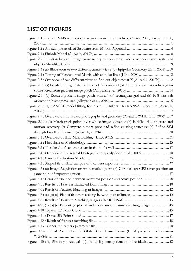
LIST OF FIGURES
Figure 1.1 : Typical MMS with various sensors mounted on vehicle (Naser, 2005; Xuexian et al.,
2009)....................................................................................................................................................... 1
Figure 1.2 : An example result of Structure from Motion Approach................................................... 4
Figure 2.1 : Pinhole Model (Al-sadik, 2012b) .......................................................................................... 8
Figure 2.2 : Relation between image coordinate, pixel coordinate and space coordinate system of
object (Al-sadik, 2012b) ...................................................................................................................... 9
Figure 2.3 : (a) Illustration of two different camera views (b) Epipolar Geometry (Zhu, 2006) ... 10
Figure 2.4 : Testing of Fundamental Matrix with epipolar lines (Kim, 2008) ................................... 12
Figure 2.5 : Overview of two different views to find out object point X (Al-sadik, 2012b) .......... 12
Figure 2.6 : (a) Gradient image patch around a key-point and (b) A 36 bins orientation histogram
constructed from gradient image patch (Alhwarin et al., 2010) .................................................. 14
Figure 2.7 : (a) Rotated gradient image patch with a 4 x 4 rectangular grid and (b) 16 8-bins sub
orientation histograms used (Alhwarin et al., 2010)...................................................................... 15
Figure 2.8 : (a) RANSAC model fitting for inliers, (b) Inliers after RANSAC algorithm (Al-sadik,
2012b) .................................................................................................................................................. 17
Figure 2.9 : Overview of multi-view photography and geometry (Al-sadik, 2012b; Zhu, 2006) ... 17
Figure 2.10 : (a) Match track points over whole image sequence (b) initialize the structure and
motion recovery (c) Compute camera pose and refine existing structure (d) Refine SfM
through bundle adjustment (Al-sadik, 2012b) ............................................................................... 20
Figure 3.1 : Overview of IIRS Main Building (IIRS, 2012) ................................................................. 21
Figure 3.2 : Flowchart of Methodology .................................................................................................. 25
Figure 3.3 : The sketch of camera system in front of a wall ................................................................ 27
Figure 3.4 : Overview of Terrestrial Photogrammetry (Aljoboori et al., 2009) ................................ 30
Figure 4.1 : Camera Calibration Sheets ................................................................................................... 35
Figure 4.2 : Shape File of IIRS campus with camera exposure station .............................................. 37
Figure 4.3 : (a) Image Acquisition on white marked point (b) GPS base (c) GPS rover position on
same point of exposure station ........................................................................................................ 37
Figure 4.4 : Error distribution between measured position and actual position............................... 38
Figure 4.5 : Results of Features Extracted from Images ...................................................................... 40
Figure 4.6 : Result of Features Matching in Images .............................................................................. 42
Figure 4.7 : (a) (b) (c) Plot of feature matching between pair of images............................................ 43
Figure 4.8 : Results of Features Matching Images after RANSAC ..................................................... 43
Figure 4.9 : (a) (b) (c) Percentage plot of outliers in pair of feature matching images ..................... 45
Figure 4.10 : Sparse 3D Point Cloud ....................................................................................................... 45
Figure 4.11 : Dense 3D Point Cloud ....................................................................................................... 47
Figure 4.12 : Result of features matching file......................................................................................... 48
Figure 4.13 : Generated camera parameter file ...................................................................................... 50
Figure 4.14 : Final Point Cloud in Global Coordinate System (UTM projection with datum
WGS84) ............................................................................................................................................... 51
Figure 4.15 : (a) Plotting of residuals (b) probability density function of residuals .......................... 52

vi
Figure 4.16 : Selected Sample Patches from Point Cloud.....................................................................53
Figure 4.17 : Group 1 dataset (a) Scattering of samples (b) Outliers in point-to-plane matching ..53
Figure 4.18 : Group 2 dataset (a) Scattering of samples (b) Outliers in point-to-plane matching ..53
Figure 4.19 : Group 3 dataset (a) Scattering of samples (b) Outliers in point-to-plane matching ..54
Figure 4.20 : (a),(b) and (c) Histogram of Points to Plane Distance for group 1, 2, 3 .....................54
Figure 4.21 : Box Plot of Group 1, 2, 3 sample dataset for points-to-plane Distance .....................55
Figure 4.22 : Position of Locators using Leica Total Station on IIRS main Building ......................57
Figure 4.23 : Difference in Easting (E), Northing (N) and Height (H) between locators
measurement and generated point clouds .......................................................................................57
Figure 4.24 : Histogram of differences in (a) Easting, (b) Northing and (c) Height Direction
between locators measurement and generated point clouds ........................................................57

vii
LIST OF TABLES
Table 1.1 : Summery of mobile mapping related sensors (Naser, 2005)......................................... 2
Table 1.2 : Function of GNSS segments along with input and output information (NRC, 1995)
................................................................................................................................................................... 3
Table 2.1 : Comparison between SIFT, SURF, PCA-SIFT (Juan et al., 2009) ............................ 13
Table 3.1 : Hardware Tools ................................................................................................................. 22
Table 3.2 : Software Tools ................................................................................................................... 23
Table 4.1 : Intrinsic Parameters of Camera and Accuracy of Calibration .................................... 36
Table 4.2 : Position of matched points in stereo image (image coordinate system) ................... 49
Table 4.3 : Rotation Matrices for exposure station 3 and 4 ............................................................ 49
Table 4.4 : Features Matched Points in local and global coordinate system ................................ 51
Table 4.5 : Transformations Parameters ............................................................................................ 51
Table 4.6 : Internal Statistics for Accuracy Assessment of Point Cloud ...................................... 55
Table 4.7 : RMSE in planimetric and depth ...................................................................................... 57

Mobile Mapping by integrating Structure from Motion approach with Global Navigation Satellite System
Page | 1
1. INTRODUCTION
1.1. Background
Since 1990s, Mobile Mapping Systems (MMS) have been started for both land and aerial digital
mapping. In comparison to conventional surveying, major developments were observed in
mobile mapping technology since the last decade by using multi sensor and real time multitasking
systems(Dorota et al., 2004). It is an emerging domain in modern data collection by integrating
various digital photogrammetry techniques and computer vision technologies such as structure
and motion (SM). Computer vision based structure and motion (SM) reconstruction for digital
photogrammetry has been used in the area of mapping for Geographic Information System (GIS)
applications providing new possibilities for the end users (Madani, 2001). The following section
explains mobile mapping system and Structure from Motion approach (SfM) in detail.
1.1.1. Terrestrial Mobile Mapping
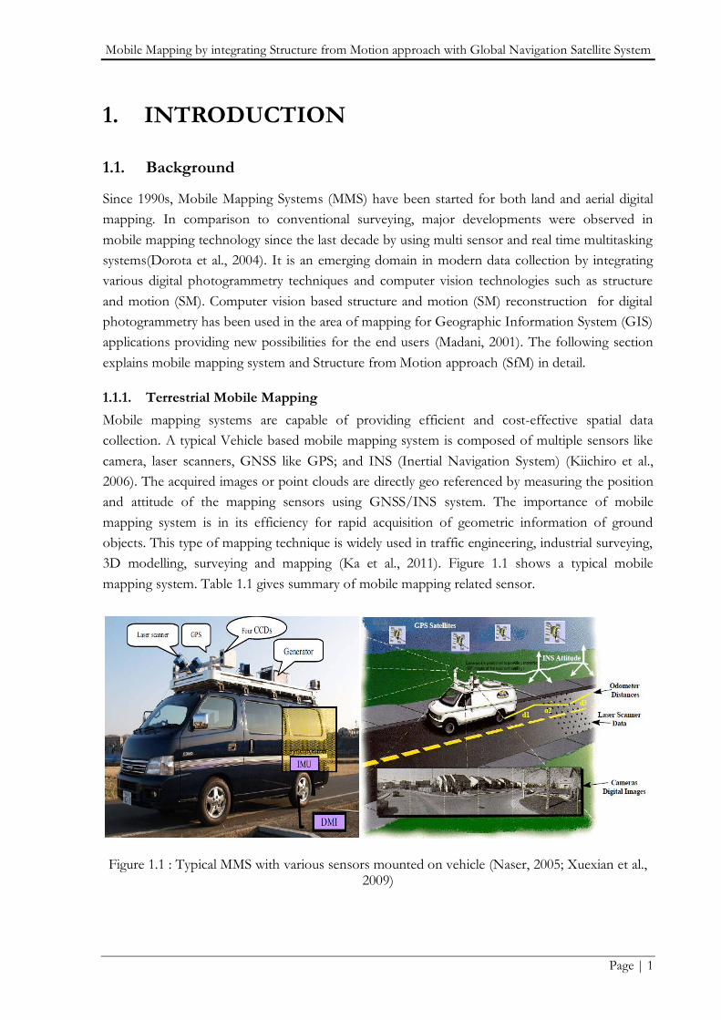
Mobile mapping systems are capable of providing efficient and cost-effective spatial data
collection. A typical Vehicle based mobile mapping system is composed of multiple sensors like
camera, laser scanners, GNSS like GPS; and INS (Inertial Navigation System) (Kiichiro et al.,
2006). The acquired images or point clouds are directly geo referenced by measuring the position
and attitude of the mapping sensors using GNSS/INS system. The importance of mobile
mapping system is in its efficiency for rapid acquisition of geometric information of ground
objects. This type of mapping technique is widely used in traffic engineering, industrial surveying,
3D modelling, surveying and mapping (Ka et al., 2011). Figure 1.1 shows a typical mobile
mapping system. Table 1.1 gives summary of mobile mapping related sensor.
Figure 1.1 : Typical MMS with various sensors mounted on vehicle (Naser, 2005; Xuexian et al., 2009)

Mobile Mapping by integrating Structure from Motion approach with Global Navigation Satellite System
Page | 2
Table 1.1 : Summery of mobile mapping related sensors (Naser, 2005)
Type of sensors Characteristics
CCD cameras Images acquisition
Imaging laser Ranging
Laser Profilers, Laser Scanners Scanning the laser data
Impulse radar Measure the thickness of objects
Ultra sonic sensors cross-section profile measurements, Road rutting
measurements
GNSS Position measurements
Inertial sensors like INS/IMU Measure position and orientation parameters
Odometers Distances
1.1.2. Global Navigation Satellite System (GNSS)
Positioning system is essential in aerial and terrestrial mapping. The aspects of GNSS introduced
here will be used for implementing the new GNSS/photogrammetric integration strategies.
GNSS can be primarily divided into three segments: Receivers, Satellites and Monitoring stations,
which are commonly termed as user, space, and control segments respectively. Table 1.2 provides
details about various segments. Modern receivers automatically track and provide outputs from
all systems which hides the control segment operations (Ellum, 2009). The popular currently
operating systems are GPS, GLONASS and Galileo. The basic differences between them are the
orbital inclination and orbital distributions. The higher orbital inclination has ground tracks that
reach higher latitudes and provides better geometry for users closer to the poles.
Global Positioning System (GPS) is very popular among all GNSS due to its well orbital
distribution. It was established by the United States DoD (Department of Defence) to provide
precise positioning system for defence and to serve the civilian community with lower accuracy.
Typical GPS receiver has some basic components like an antenna, RF (radio frequency) section, a
microprocessor, a CDU (control and display unit), recording device and a power supply (NRC,
1995). Each GPS satellite continuously transmits signals information like navigation messages to
measure the position. The user segment needs at least 4 satellites for proper positioning. There
are two methods of single receiver GPS positioning: static and dynamic. The level of accuracy in
both cases is in meter level. Thus there is a need of better accuracy to do mapping accurately and
it can be achieved by using Differential GPS system to increase the mapping accuracy in cm level.
Differential GPS (DGPS) positioning is a technique which provides accuracy at centimetre level
depending on several key factors including the use of two different GPS receivers. One receiver
is called base or reference receiver and the second receiver is called roving receiver or rover. The
base station is placed at a point where the exact position is already known very accurately, where
as the rover moves over the points to be positioned. There are mainly four methods of DGPS
positioning: static-post processing, static-real time processing, dynamic-with real time processing

Mobile Mapping by integrating Structure from Motion approach with Global Navigation Satellite System
Page | 3
and dynamic-with post processing. At each point, the satellite data from at least 4 separate
satellites is stored in the receiver. Meanwhile, the base also tracks the same satellite and records
similar data, but for two different location. Thus at the same time, both the base and rover
receivers track the same satellites and store similar data which provides centimetre level accuracy
in both 2D and 3D (NRC, 1995). This level of accuracy is often desirable to measure point, lines
and polygon for a Geographic Information System (GIS) or for mapping purpose.
Table 1.2 : Function of GNSS segments along with input and output information (NRC, 1995)
Segment Input Output Functions
Space Navigation Message
Navigation Message
transmits on
P (pseudo) and C/A Code,
L1(1575.42 MHz), L2
(1227.60 MHz) carrier
Generate code, carrier phase
to transmit navigation
message
Control P-Code observation time Navigation Message
Product GNSS time, predict
ephemeris,
manage space vehicles
User
Carrier Phase Observation,
Code observation,
Navigation Message
Position, Velocity, Time Surveying and Navigation
Solution
1.1.3. Structure from Motion Approach (SfM)
Structure from Motion (SfM) makes it possible to generate 3D point clouds from images. SfM
technique is simultaneous recovery of 3D points and camera projection matrices using
corresponding 2D image points/feature points in multiple views (Sabzevari et al., 2011). It‟s not
possible to extract each and every point from 2D images. Thus there is a need of feature
extraction and matching of key points from sequence of images. There are various local
descriptors available for feature extraction and matching (Mikolajczyk et al., 2005). Matched
features in multiple views are used with bundle adjustment to build a sparse three dimensional
point cloud of the viewed scene using projection matrices and also simultaneously estimates
camera poses and calibration parameters. Thus this whole process is known as Structure from
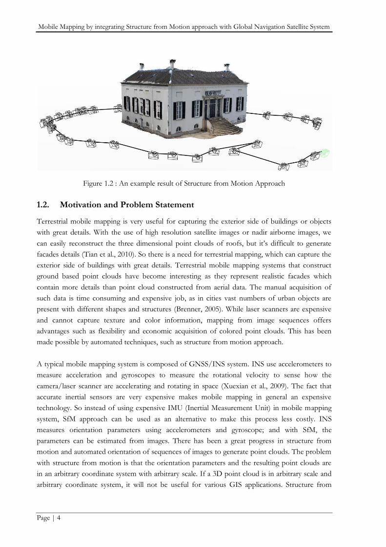
Motion approach. Figure 1.2 shows the basic idea of Structure from Motion (SfM) Approach. In
this figure, dense object‟s point cloud is shown in RGB color along with the trajectory of camera
exposure stations.
Mobile Mapping by integrating Structure from Motion approach with Global Navigation Satellite System
Page | 4
Figure 1.2 : An example result of Structure from Motion Approach
1.2. Motivation and Problem Statement
Terrestrial mobile mapping is very useful for capturing the exterior side of buildings or objects
with great details. With the use of high resolution satellite images or nadir airborne images, we
can easily reconstruct the three dimensional point clouds of roofs, but it‟s difficult to generate
facades details (Tian et al., 2010). So there is a need for terrestrial mapping, which can capture the
exterior side of buildings with great details. Terrestrial mobile mapping systems that construct
ground based point clouds have become interesting as they represent realistic facades which
contain more details than point cloud constructed from aerial data. The manual acquisition of
such data is time consuming and expensive job, as in cities vast numbers of urban objects are
present with different shapes and structures (Brenner, 2005). While laser scanners are expensive
and cannot capture texture and color information, mapping from image sequences offers
advantages such as flexibility and economic acquisition of colored point clouds. This has been
made possible by automated techniques, such as structure from motion approach.
A typical mobile mapping system is composed of GNSS/INS system. INS use accelerometers to
measure acceleration and gyroscopes to measure the rotational velocity to sense how the
camera/laser scanner are accelerating and rotating in space (Xuexian et al., 2009). The fact that
accurate inertial sensors are very expensive makes mobile mapping in general an expensive
technology. So instead of using expensive IMU (Inertial Measurement Unit) in mobile mapping
system, SfM approach can be used as an alternative to make this process less costly. INS
measures orientation parameters using accelerometers and gyroscope; and with SfM, the
parameters can be estimated from images. There has been a great progress in structure from
motion and automated orientation of sequences of images to generate point clouds. The problem
with structure from motion is that the orientation parameters and the resulting point clouds are
in an arbitrary coordinate system with arbitrary scale. If a 3D point cloud is in arbitrary scale and
arbitrary coordinate system, it will not be useful for various GIS applications. Structure from

Mobile Mapping by integrating Structure from Motion approach with Global Navigation Satellite System
Page | 5
Motion (SfM) technique is used in a variety of applications including town planning, remote
measurement, photogrammetric survey and in the creation of automatic reconstruction of
virtually real environments from video sequences or sequence of images (Zhang et al., 2005).
Therefore, this study attempts to construct 3D cloud points by integrating GNSS/ SFM which
will be used for above mentioned applications and makes a mobile mapping system that is not
expensive compared to GNSS/INS and also provides geo-referenced data in a correct scale with
the use of GNSS.
1.3. Research Identification
1.3.1. Research Objectives
My research topic focuses on the feasibility of mapping by integrating Structure from Motion
approach, which estimates camera orientation parameters from the images, and GNSS which
provides scale.
Sub-objectives:
To check the reliability of feature extraction and matching to find the correct
corresponding features from the sequence of overlapping images.
To generate point clouds on the basis of image matching and image orientation.
To implement a method for the integration of GNSS and structure from motion
approach to introduce the correct scale and geo reference the point cloud from acquired
images.
To perform the quantitative analysis of the point cloud using internal and external
accuracy assessments.
1.3.2. Research Questions
To reach the above objective the following questions need to be answered.
1. How reliable are the SIFT and RANSAC algorithms to extract and match
proper/correct corresponding features from sequence of overlapping images?
2. How to integrate GPS measurement with the corresponding feature points to make the
whole system geo referenced and introduce a proper scale in three dimensional point
cloud?
3. How to assess the quality of generated point cloud? What is the accuracy of generated
point cloud?

Mobile Mapping by integrating Structure from Motion approach with Global Navigation Satellite System
Page | 6
1.4. Thesis Structure
The research work is organized as follows:
Chapter 1: Introduction, this section presents general overview about the research work. It
describes the basic idea of topic, motivation, problem statement, research objectives, and
research questions.
Chapter 2: Theoretical Background and Literature Review, this chapter deals with theoretical
background of the study and literature review. It also explains various components of computer
vision digital photogrammetry.
Chapter 3: Materials and Methodology, this chapter describes the complete workflow of the study
and description in details, about data used, hardware and software tools used.
Chapter 4: Results and Evaluations, this chapter describe the experiments on selected data,
achieved results, its discussion and analysis.
Chapter 5: Conclusion and Recommendation, this section describes the answer of the research
questions in concluded form and recommendations for further study.

Mobile Mapping by integrating Structure from Motion approach with Global Navigation Satellite System
Page | 7
2. LITERATURE REVIEW AND THEORETICAL BACKGROUND
Mapping of man-made object from aerial images has already been a topic of interest from many
years (Remondino et al., 2006). But the problem that lies in satellite and aerial images of urban
area is that only the roof (top view) can be well observed in these images and not the facades. In
recent years, there has been an interest in developing methods for generating three dimensional
data using the combination of satellite/aerial images, 2D map data and terrestrial data to improve
the reliability and accuracy of the mapping system (Zhang et al., 2005).
Till now lots of work has been done on mapping of real objects and scenes from terrestrial
platforms. For terrestrial mobile mapping, there are mainly two methods. One is based on active
range data e.g. laser scanning and other is based upon video images or image sequences. Active
range based mapping methods are very useful to directly capture 3D geometric information with
highly detailed and accurate representation of shapes (Pu et al., 2009). Laser scanner integration
with IMU (Inertial Measurement Unit)/GPS provides directly the measurement of dense point
clouds in global coordinate system but it does not give surface information like texture in laser
point clouds (Xuexian et al., 2009). Another data acquisition technique is based on CCD (charge-
coupled device) camera integration with INS/GPS system. Piras et al. (2008) developed a
integrated systems with GNSS, IMU, video camera that allows quick and accurate mapping. The
GNSS with IMU integration for the derivation of the position and attitude angles of the mapping
vehicle is usually based on Kalman filter. It allows the position of the exposure station to be
surveyed, even in the loss of a GNSS signal (Piras et al., 2008). These types of data acquisition
techniques rely on expensive inertial sensors. Another method for mapping surrounding scene is
by camera integration with GNSS and SfM (Structure from Motion) approach to overcome the
cost of the whole system.
Structure from Motion (SfM) makes it possible to generate 3D point clouds from images with
camera projection matrices using corresponding 2D image points in multiple views (Sabzevari et
al., 2011). It uses corresponding image points in multiple views and a 3D point can be
reconstructed by triangulation. An important requirement is the measurement of camera pose
and calibration, which may be expressed by a projection matrix of each camera. But it‟s not
possible to compare each and every pixel of one image with next image. In addition to this, there
is no guarantee that each and every point is equally well suited for automatic matching (Pollefeys
et al., 2000). So there is a need of feature extraction in image processing as a part of special form
of dimensionality reduction. Common method for feature extraction, matching and outliers‟
removal between wrong feature matches are Scale Invariant Feature Transform (SIFT) (Lowe,
1999), Approximate Nearest Neighbours (ANN) (Arya et al., 2010) and RANdom Sample
Consensus (RANSAC) respectively (Fischler et al., 1981) which are widely used by many
Mobile Mapping by integrating Structure from Motion approach with Global Navigation Satellite System
Page | 8
researchers and is known to perform well over a reasonable range of viewpoint variations.
Extracted and matched features in multiple views are used with bundle adjustment to build a
sparse three dimensional point cloud of the viewed scene to simultaneously recover camera poses
and calibration parameters. Triggs et al. (2000) reviewed bundle adjustment technique which is a
widely used technique to estimate camera pose and produced 3D point clouds from image
correspondences. Bundle adjustment is used as the last step in feature based multi-view structure
and motion estimation algorithm (Lourakis et al., 2009). Thus the simultaneous recovery of 3D
points and camera projection matrices using corresponding 2D image points in multiple views is
known as the structure from motion.
The following section will explain SfM techniques in details, by describing the theoretical
background and research on projection matrices (camera parameters), epipolar geometry, feature
extraction, matching and bundle adjustment. First two sections give the overview of camera
parameters and simple concept of epipolar geometry which is used in SfM to estimate the
position of object point in 3D space.
2.1. Camera Parameters
2.1.1. Pinhole Model
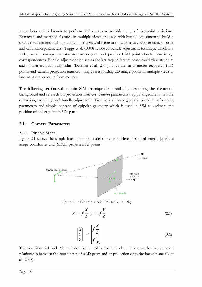
Figure 2.1 shows the simple linear pinhole model of camera. Here, f is focal length, [x, y] are
image coordinates and [X,Y,Z] projected 3D points.
Figure 2.1 : Pinhole Model (Al-sadik, 2012b)
𝑥 = 𝑓𝑋
𝑍, 𝑦 = 𝑓
𝑌
𝑍 (2.1)
𝑋𝑌𝑍 →
𝑓𝑋
𝑍
𝑓𝑌
𝑍
(2.2)
The equations 2.1 and 2.2 describe the pinhole camera model. It shows the mathematical
relationship between the coordinates of a 3D point and its projection onto the image plane (Li et
al., 2008).

Mobile Mapping by integrating Structure from Motion approach with Global Navigation Satellite System
Page | 9
2.1.2. Intrinsic and Extrinsic Parameters
The intrinsic parameters are focal length, principal points, lens distortions parameters. Extrinsic
parameters define the position of the exposure station and camera orientation parameters in
world coordinate system. Figure 2.2 shows relation between image coordinate, pixel coordinate
and space coordinate system of object. Equation 2.4 shows relation between image coordinate to
pixel coordinate.
Figure 2.2 : Relation between image coordinate, pixel coordinate and space coordinate system of object (Al-sadik, 2012b)
𝑝 = 𝐾𝑖𝑛𝑡 ∗ 𝑚 (2.3)
𝑢𝑣1 =
𝑓 0 uo
0 𝑓 vo
0 0 1
𝑥𝑦1 (2.4)
where, 𝐾𝑖𝑛𝑡 is matrix of intrinsic parameters, p(u, v) is in pixel coordinates system, m(x, y) is in
image coordinate system and (uo, vo) is principal point.
Equation 2.5 explains relationship between world 3D coordinates of object to camera coordinate
system. Equation 2.6 shows the rotation and translation matrices.
𝑋𝐿
𝑌𝐿𝑍𝐿
= 𝑅 𝑋𝐴
𝑌𝐴𝑍𝐴
− 𝑇 (2.5)
𝑅 =
𝑟11 𝑟12 𝑟13
𝑟21 𝑟22 𝑟23
𝑟31 𝑟32 𝑟33
, T =
𝑡1
𝑡2
𝑡3
(2.6)
where, coordinates of exposure station are XL, YL, ZL in world coordinate system. Coordinates of
object point A is XA, YA, ZA. R and T denotes as rotation and translation matrices respectively. R
is a function of rotation angles ω, φ, қ around the x, y, z axes respectively.

Mobile Mapping by integrating Structure from Motion approach with Global Navigation Satellite System
Page | 10
2.1.3. Projection Matrix
Projection matrix relates the pixel coordinate system to world coordinate system. Equation for
projection matrixes are defined as below,
𝑥 = 𝐾𝑖𝑛𝑡 ∗ 𝐾𝑒𝑥𝑡 ∗ 𝑋 (2.7)
where 𝐾𝑒𝑥𝑡 denotes extrinsic parameters.
𝑥 = 𝐾𝑖𝑛𝑡 ∗ 𝑅 𝐼 − 𝑇] ∗ 𝑋 → 𝑥 = 𝑃𝑋 (2.8)
where P is a projection matrix, I is an identity matrix.
𝑢𝑣1 =
𝑝11 𝑝12 𝑝13
𝑝21 𝑝22 𝑝23 𝑝31 𝑝32 𝑝33
𝑝14
𝑝24
𝑝34
∗
𝑋𝑌𝑍1
(2.9)
Projection matrix can be solved by singular value decomposition (SVD) using direct linear
transformation algorithm (DLT). P is a 3 x 4 matrix which has 7 degree of freedom (1 for focal
length, 3 from rotation and 3 from translation)
2.1.4. Epipolar Geometry
Epipolar geometry is the stereo view of two cameras when cameras view a 3D object from two
different locations. There are numbers of geometry relation between the 3D object points and
their projection onto 2D images to estimate the position of the 3D object. Zhu (2006) gives short
description for multiple view geometry in computer vision from well known book of Zisserman
et al. (2001). Figure 2.3 (a),(b) show the example of two different camera view (stereo).
(a) (b)
Figure 2.3 : (a) Illustration of two different camera views (b) Epipolar Geometry (Zhu, 2006)
Consider an image point p in the first left side image and q is the corresponding point right side
image. Two special points‟ e1 and e2 are epipoles which show the projection of one camera into
other. All of the epipolar lines in an image pass through epipole. The epipolar geometry of two
views is described by 3x3 Fundamental Matrix (F).
𝐹 =
𝑓11 𝑓12 𝑓13
𝑓21 𝑓22 𝑓23
𝑓31 𝑓32 𝑓33
(2.10)
Mobile Mapping by integrating Structure from Motion approach with Global Navigation Satellite System
Page | 11
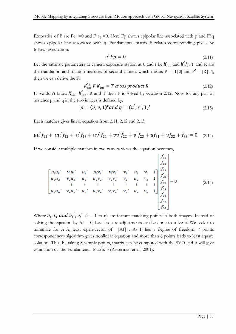
Properties of F are Fe1 =0 and FTe2 =0. Here Fp shows epipolar line associated with p and FTq
shows epipolar line associated with q. Fundamental matrix F relates corresponding pixels by
following equation.
𝑞𝑡𝐹𝑝 = 0 (2.11)
Let the intrinsic parameters at camera exposure station at 0 and t be 𝐾𝑖𝑛𝑡 and 𝐾𝑖𝑛𝑡′ 𝑡 . T and R are
the translation and rotation matrices of second camera which means P = [I|0] and P′ = [R|T],
then we can derive the F:
𝐾𝑖𝑛𝑡′ 𝑡 𝐹 𝐾𝑖𝑛𝑡 = 𝑇 𝑐𝑟𝑜𝑠𝑠 𝑝𝑟𝑜𝑑𝑢𝑐𝑡 𝑅 (2.12)
If we don‟t know 𝐾𝑖𝑛𝑡 , 𝐾𝑖𝑛𝑡′ , R and T then F is solved by equation 2.12. Now for any pair of
matches p and q in the two images is defined by,
𝑝 = 𝑢, 𝑣, 1 𝑡𝑎𝑛𝑑 𝑞 = (𝑢′ , 𝑣 ′ , 1)𝑡 (2.13)
Each matches gives linear equation from 2.11, 2.12 and 2.13,
𝑢𝑢′𝑓11 + 𝑣𝑢′𝑓12 + 𝑢′𝑓13 + 𝑢𝑣 ′𝑓21 + 𝑣𝑣 ′𝑓22 + 𝑣 ′𝑓23 + 𝑢𝑓31 + 𝑣𝑓32 + 𝑓33 = 0 (2.14)
If we consider multiple matches in two camera views the equation becomes,
(2.15)
Where 𝑢𝑖 , 𝑣𝑖 𝑎𝑛𝑑 𝑢𝑖′ , 𝑣𝑖
′ (i = 1 to n) are feature matching points in both images. Instead of
solving the equation by Af = 0, Least square adjustments can be done to solve it. We seek f to
minimize for ATA, least eigen-vector of ||Af||. As F has 7 degree of freedom. 7 points
correspondences algorithm gives nonlinear equation and more than 8 points leads to least square
solution. Thus by taking 8 sample points, matrix can be computed with the SVD and it will give
estimation of the Fundamental Matrix F (Zisserman et al., 2001).

Mobile Mapping by integrating Structure from Motion approach with Global Navigation Satellite System
Page | 12
Figure 2.4 : Testing of Fundamental Matrix with epipolar lines (Kim, 2008)
As the fundamental matrix can be computed using the intrinsic parameters 𝐾𝑖𝑛𝑡 and 𝐾𝑖𝑛𝑡′ 𝑡 and the
8 correspondences, [𝑥 ′ ←→ 𝑥 ], which can be estimated as the projection matrix (relative
translation and rotation) of two cameras.
P = [I|0] and P′ = [R|T] (2.16)
Projection matrixes of both camera P1 and P2 are available at O1 and O2, corresponding 2D
points are (u1, v1) and (u2, v2). By using multiple view triangulations, X can be found. Figure 2.5
shows general overview to find object point X and equation 2.17 gives the idea to find out object
point X.
Figure 2.5 : Overview of two different views to find out object point X (Al-sadik, 2012b)

Mobile Mapping by integrating Structure from Motion approach with Global Navigation Satellite System
Page | 13
Equation 2.17 : Solution for 3D point X from projection matrices (Al-sadik, 2012b)
Till now it has been discussed about the two view geometry and manual extraction of
corresponding image points from images. There is a need of automation for image point
extraction and find out 3D point of object in multiple view geometry with estimation of camera
orientation parameters.
2.2. Feature Extraction and Matching
Researchers have developed various algorithms for extracting feature and matching them in the
overlapped images. Mikolajczyk et al. (2005) compared the performance of various local
descriptors which is used to recall and precise the evaluation criterion to give the experiments of
comparison for affine transformations, scale changes, rotation, blur, compression, and
illumination changes. Comparative study of SIFT, Principal Component Analysis (PCA) - SIFT
and Speeded Up Robust Features (SURF) is given by Juan et al. (2009). In these experiments,
ANN was used to find the matches, and RANSAC to reject inconsistent matches (outliers) from
which the inliers can take as correct features matches and Table 2.1 shows their experiments
results.
Table 2.1 : Comparison between SIFT, SURF, PCA-SIFT (Juan et al., 2009) Method Time Scale Illumination Rotation Blur Affine
SIFT common best common best best Good
SURF best good good common good Good
PCA-SIFT good common best good common Good

Mobile Mapping by integrating Structure from Motion approach with Global Navigation Satellite System
Page | 14
In this experiment, SURF uses „Fast-Hessian‟ detector, which is 3 times faster than DoG
(Difference of Gaussian) which was used in SIFT and 5 times faster than Hessian Laplace (Bay et
al., 2006). SURF does not show good performance in rotation. In Table2.1, we can make out that
PCA-SIFT has low performance for blur and scale. The performance of SIFT is stable in all the
experiments excluding time, because it detects many key-points features and finds many matches.
Yan et al. (2004) claims that PCA-SIFT is well suited to represent patches of key-points but it‟s
sensitive to registration errors. Zhan-long et al. (2008) used SIFT as an automatic image mosaic
technique.
SIFT method developed by Lowe (1999, 2001, 2004) transforms the image into a set of local
features which are extracted through the three stages: feature detection and their linearization,
feature orientation assignment and feature descriptor.
1. Feature detection and their localization: Extrema of DoG scale space is used to select
the locations of potential interest points in the image. To search scale space extrema in
the DoG images, each pixel is compared with its 26 neighbours in 3×3 regions of scale
space. The pixel is compared with all its neighbours; if the pixel is lower or lager than
neighbouring pixel, then it is marked as a candidate key-point. By using second order
Taylor expansions around key-points, each of these key-points is exactly localized by
fitting a three dimensional quadratic functions. Then key-points of low contrast and
points that belong to edges are discarded.
2. Feature orientation assignment: An orientation of key-point is assigned based on local
image gradient data. For each pixel of image region around the candidate key-point, the
first order gradient (magnitude and orientation) is calculated. This gradient data is
weighted by scale dependent Gaussian window which is illustrated by a circular window
in figure 2.6(a). It is then used to build a 36 bin orientation histogram covering the range
of orientations [ -180°, 180° ] as shown in figure 2.6 (b). The orientation of the SIFT
feature θmax is defined as the orientation corresponding to the maximum bin of the
orientation histogram as shown in figure 2.6 (Alhwarin et al., 2010).
Figure 2.6 : (a) Gradient image patch around a key-point and (b) A 36 bins orientation histogram constructed from gradient image patch (Alhwarin et al., 2010)
Mobile Mapping by integrating Structure from Motion approach with Global Navigation Satellite System
Page | 15
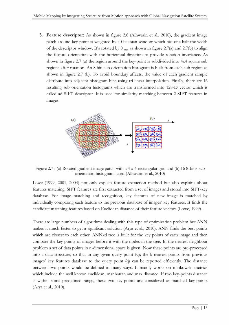
3. Feature descriptor: As shown in figure 2.6 (Alhwarin et al., 2010), the gradient image
patch around key-point is weighted by a Gaussian window which has one half the width
of the descriptor window. It‟s rotated by θ max as shown in figure 2.7(a) and 2.7(b) to align
the feature orientation with the horizontal direction to provide rotation invariance. As
shown in figure 2.7 (a) the region around the key-point is subdivided into 4x4 square sub
regions after rotation. An 8 bin sub orientation histogram is built from each sub region as
shown in figure 2.7 (b). To avoid boundary affects, the value of each gradient sample
distribute into adjacent histogram bins using tri-linear interpolation. Finally, there are 16
resulting sub orientation histograms which are transformed into 128-D vector which is
called ad SIFT descriptor. It is used for similarity matching between 2 SIFT features in
images.
Figure 2.7 : (a) Rotated gradient image patch with a 4 x 4 rectangular grid and (b) 16 8-bins sub orientation histograms used (Alhwarin et al., 2010)
Lowe (1999, 2001, 2004) not only explain feature extraction method but also explains about
features matching. SIFT features are first extracted from a set of images and stored into SIFT-key
database. For image matching and recognition, key features of new image is matched by
individually comparing each feature to the previous database of images‟ key features. It finds the
candidate matching features based on Euclidean distance of their feature vectors (Lowe, 1999).
There are large numbers of algorithms dealing with this type of optimization problem but ANN
makes it much faster to get a significant solution (Arya et al., 2010). ANN finds the best points
which are closest to each other. ANNkd tree is built for the key points of each image and then
compare the key-points of images before it with the nodes in the tree. In the nearest neighbour
problem a set of data points in n-dimensional space is given. Now these points are pre-processed
into a data structure, so that in any given query point (q); the k nearest points from previous
images‟ key features database to the query point (q) can be reported efficiently. The distance
between two points would be defined in many ways. It mainly works on minkowski metrics
which include the well known euclidean, manhattan and max distance. If two key-points distance
is within some predefined range, these two key-points are considered as matched key-points
(Arya et al., 2010).

Mobile Mapping by integrating Structure from Motion approach with Global Navigation Satellite System
Page | 16
Alhwarin et al. (2010) has developed a new method VF-SIFT (Very Fast SIFT) of feature
matching. The idea behind is to extend a SIFT feature by 4 pair wise independent angles. These
angles are invariant to rotation, scale and illumination changes. SIFT features are classified based
on their angles into different clusters during the feature extraction phase. These angles are used
for feature matching together with SIFT descriptors. Thus we can neglect the comparison of the
portion of features that can‟t be matched in any way. It will lead to speed up matching
techniques.
The result of features matching algorithm contains a lot of outliers between matched features
which needs to be removed. Sunglok et al. (2009) describes comparison between outliers‟
removal family like MLESAC (Maximum Likelihood SAmple Consensus), MAPSAC (Maximum
A Posterior Estimation SAmple Consensus), MSAC (M-estimator SAmple Consensus),
RANSAC. The comparison was done on the basis of accuracy, computing time, and robustness.
RANSAC, MSAC and MLESAC‟s accuracy have differed nearly by 4%. MSAC has considered to
be the most accurate among three estimators, and MLESAC is found to be the worst. The
performance of MAPSAC is found to be similar with line fitting experiments. Its accuracy was is
also similar with RANSAC.
The RANdom SAmple Consensus (RANSAC) algorithm, originally introduced by Fischler et al.
(1981). Yaniv (2010) describes that RANSAC algorithm is based on the observation that if we
can draw a small subset from the data set to estimate the RANSAC model parameters and which
contains no outliers, then all inliers will agree with this model. This is done by, estimating
corresponding models from randomly drawing data subsets and assessing how many data
elements agree with each and every model with its consensus set. The maximal consensus set
obtained in this manner is assumed to be outlier free. It‟s used as input for least squares model
estimate. The basic algorithm of RANSAC is summarized below by Derpanis (2010) and the
main steps are written below:
1. Minimum numbers of points are selected randomly to determine the model parameters.
2. Parameters of the model are solved.
3. Now check number of points from the set of all points fit with a predefined tolerance.
4. If the set of number of inliers over the total numbers points exceeds a predefined
threshold, then restart the estimation of the model parameters using all the identified
inliers and terminate.
5. Otherwise, repeat steps from 1 to 4 up to maximum of N iterations.
The number of iterations N is chosen high enough to ensure that the probability is near to one
(0.95). It means that at least one of the sets of random sample does not include any outliers.
Assume u is the probability that any selected data point is an inlier. Thus v = 1 − u is the
probability of observing an outlier. There are N iterations of the minimum number of points
denoted m are required,

Mobile Mapping by integrating Structure from Motion approach with Global Navigation Satellite System
Page | 17
1 − 𝑝 = (1 − 𝑢𝑚 )𝑁 (2.18)
and thus with some manipulation N is obtained by following equation,
𝑁 = log(1 − 𝑝)
log(1 − 1 − 𝑣 𝑚 ) (2.19)
The Figure 2.8(a) shows how the RANSAC algorithm selects the one model with the largest
number of inliers from all possible lines. Figure 2.8(b) shows inliers after RANSAC algorithm.
(a) (b)
Figure 2.8 : (a) RANSAC model fitting for inliers, (b) Inliers after RANSAC algorithm (Al-sadik, 2012b)
2.3. Multiple view Geometry for SfM
Multiple view geometry is broadly described in Zisserman et al. (2001)‟s book. The following
section will describe brief overview of multiple view geometry to find out camera projection
matrices and position of 3D object X as shown in Figure 2.9.
Figure 2.9 : Overview of multi-view photography and geometry (Al-sadik, 2012b; Zhu, 2006)
Consider 𝑄𝑖 {𝑄1,𝑄2, . . , 𝑄𝑚} are images with reasonable overlap between images. Projection
matrices are 𝑃𝑖 { 𝑃1 , 𝑃2 , . . , 𝑃𝑚 } as described earlier in section 2.1.3, where each

Mobile Mapping by integrating Structure from Motion approach with Global Navigation Satellite System
Page | 18
𝑃𝑖 = 𝐾𝑖 [𝑅𝑖|𝑇𝑖 ], 𝐾𝑖 is intrinsic parameters, 𝑅𝑖𝑎𝑛𝑑 𝑇𝑖 are rotation and translation matrices
respectively.
𝑥𝑖𝑗 = 𝑃𝑖𝑋𝑗 (2.20)
where, 𝑖 = 1, … , 𝑚 𝑎𝑛𝑑 𝑗 = 1, . . , 𝑛. Here „m‟ images are available with reasonable overlaps of
„n‟ rigid 3D points. If the image measurements are noisy, the projection does not satisfy exactly.
𝑃 𝑖𝑋 𝑗 ≠ 𝑥𝑖𝑗 (2.21)
where, 𝑃 𝑖 is the set of camera matrices and 𝑋 𝑗 is set of points.
Estimate the projection matrices 𝑃 𝑖 and 3D points 𝑋 𝑗 which are projected exactly to image
point 𝑥𝑖𝑗 . Bundler Adjustment (Triggs et al., 2000) will minimize distance between estimated 𝑥 𝑖𝑗
and measured 𝑥𝑖𝑗 points for every view by using.
min𝑃𝑖 ,𝑥𝑗
𝑑(
𝑖𝑗
𝑃 𝑖𝑋 𝑗 , 𝑥𝑖𝑗 )2 (2.22)
where, 𝑑(𝑃 𝑖𝑋 𝑗 , 𝑥𝑖𝑗 ) is the geometric image distance between homogenous point
𝑃 𝑖𝑋 𝑗 𝑎𝑛𝑑 𝑥𝑖𝑗 .
min 𝑃 𝑖𝑋 𝑗 will adjust the bundle of rays between each camera centre and 3D points and vice
versa. Lease square optimization uses iterative solution to find the parameters P that minimize
the difference between the measure 𝑥 and estimated 𝑥 .
There are different strategies for bundle adjustment. The basic strategy for bundle adjustment
algorithm are followed by this step (Zhu, 2006):
1. Find the M tracks M = {M1, M2,.., MN}
a. Take pair of images {𝑄𝑖 , 𝑄𝑗}, 𝑖 ≠ 𝑗:
i. Detect and extract the SIFT feature point in 𝑄𝑖 , 𝑄𝑗
ii. Feature matching across images and outliers‟ removal using RANSAC
b. Again matching features across multiple images and construct tracks for that {M1,
M2,.., MN}
2. Estimation of 𝑃𝑖 {𝑃1, 𝑃2, . . , 𝑃𝑚} and 3D position for each track
a. Select first pair of images {𝑄1 , 𝑄2 } and consider M1‟2‟ are their associative
overlapping tracks
b. Estimate 𝐾1′ and 𝐾2′ intrinsic parameters and compute { 𝑃1, 𝑃2 } and 3D
position of M1‟2‟ from fundamental matrix.
c. Incrementally add new camera 𝑃𝑘 into the system and estimate its camera
projection matrices by direct linear transformation algorithm (DLT) and refine
the existing structure.

Mobile Mapping by integrating Structure from Motion approach with Global Navigation Satellite System
Page | 19
d. Initialize new structure points and repeat (c) until all camera parameters are
estimated. Refine all structure and motion through bundle adjustment.
But there is possibility of re-projection error in projection matrices which is minimized by
nonlinear least-squares algorithms, such as Levenberg-Marquardt (LM) iteration algorithm
(Madsen et al., 2004). It minimizes the re-projection error and non-linearly optimizes the system.
Lourakis et al. (2009)‟s sparse bundle adjustment uses LM algorithm and bundle adjustment
(Triggs et al., 2000) for estimation of camera parameters and 3D point of object.
As presented in Lourakis et al. (2009), the LM algorithm is an insistent technique that determines
a local minimum of a multivariate function that is formulated as the sum of squares of several
nonlinear, real valued functions. Thus it has become a standard approach for nonlinear least-
squares problems, widely accepted in various fields for dealing with data-fitting applications. LM
algorithm can be regarded as an aggregation of steepest descent and the Gauss Newton Method.
When the accepted solution is outlying from a local minimum, then the algorithm behaves like a
steepest descent method: slow, but it‟s guaranteed to converge. When the current solution is
close to a local minimum, then it becomes a Gauss Newton method and exhibits fast
concurrence.
As presented in Lourakis et al. (2009), Sparse Bundle Adjustment is a classic method for
optimizing a structure-from-motion problem in Computer Vision where it optimizes a set of
camera poses and visible points. Each camera frame consists of a translation and rotation giving
the position and orientation of the frame in global coordinates. Bundle Adjustment attempts to
filter the visual reconstruction to produce optimal 3D structure in conjunction with viewing
parameter estimates. Optimal refers to minimizing (or maximizing) a cost function that
determines the model fitting error with respect to both camera and structure adaptations. The
name refers to the „bundle‟ of light rays leaving each 3D feature and converge on each camera
centre, which are adapted optimally with respect to both feature and camera positions. Bundle
adjustment (BA) understates the re-projection error between the detected and foreboded image
points, which is expressed as the sum of squares of a large number of nonlinear, real valued
functions. Thus, the minimization is attained using nonlinear least-squares algorithms, for which
Levenberg-Marquardt (LM) has proven to be the most productive due to its ease of
implementation and its use of an effective damping strategy that adds to it the ability to converge
quickly from a wide range of initial guesses. This algorithm is first shown to be a blend of vanilla
gradient descent and Gauss-Newton iteration. Here the damping term is used at each iteration to
ensure a reduction in error. The problem for which the LM algorithm provides a solution is
called Nonlinear Least Squares Minimization.
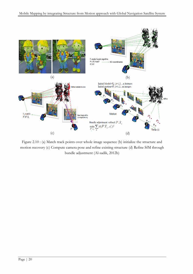
Figure 2.10 show whole SfM workflow in step by step from a to d.
Mobile Mapping by integrating Structure from Motion approach with Global Navigation Satellite System
Page | 20
(a)
(b)
(c) (d)
Figure 2.10 : (a) Match track points over whole image sequence (b) initialize the structure and
motion recovery (c) Compute camera pose and refine existing structure (d) Refine SfM through
bundle adjustment (Al-sadik, 2012b)

Mobile Mapping by integrating Structure from Motion approach with Global Navigation Satellite System
Page | 21
3. MATERIALS AND METHODOLOGY
In this thesis, the feasibility of integration of SfM approach and GNSS using space photo
intersection and point-based similarity transformation method for mapping is studied. To achieve
the objectives, test scene was selected and various hardware-software tools were used in present
study. The following sections describe the methodology adopted in details along with test scene,
hardware-software tools used.
3.1. Study Area and Data
IIRS (Indian Institute of Remote Sensing) main building is used as a test scene. IIRS is formerly
known as Indian Photo-interpretation Institute (IPI), the Institute was founded on 21st April
1966 under the aegis of Survey of India (SOI). It was established with the collaboration of the
Government of The Netherlands on the pattern of Faculty of Geo-Information Science and
Earth Observation (ITC) of the University of Twente, formerly known as International Institute
for Aerospace Survey and Earth Sciences, The Netherlands. The original idea of setting the
Institute came from India's first Prime Minister Pandit Jawahar Lal Nehru during his visit to The
Netherlands in 1957(IIRS, 2012). Thus there is a very good history of my test scene. The
Institute's building at Kalidas Road, Dehradun, India was inaugurated on May 27, 1972. The
average height of building is 652m in geodetic coordinate system with datum WGS84. Here field
work would only involve data acquisition like taking images from different angles and recording
DGPS measurements for a test scene. Figure 3.1 shows the overview of IIRS main building.
Figure 3.1 : Overview of IIRS Main Building (IIRS, 2012)

Mobile Mapping by integrating Structure from Motion approach with Global Navigation Satellite System
Page | 22
3.2. Tools Used
3.2.1. Hardware Tools
Table 3.1 gives the detail of hardware used for the research work.
Table 3.1 : Hardware Tools
S.
No. Hardware Model No. Used for
1 Camera Nikon D-80 SLR Capturing images
2 DGPS system Leica GPS 510 with base and
rover (single frequency)
Measure position of exposure
station
3 Total Station Leica TPS 1200 Evaluation of point cloud (for
marking locators)
4 Measuring Tape,
Plumb-bob Standard (30 m), Standard
Object measurements and for
centring tripod respectively.
5 Laptop Sony Vaio (Intel Core i3, 64
bit, 2.10GHz, 4 GB RAM) Processing work

Mobile Mapping by integrating Structure from Motion approach with Global Navigation Satellite System
Page | 23
3.2.2. Software Tools
Different software was used for the successful execution of this study. Table 3.2 shows the lists
of software/packages used to execute different tasks during my study:
Table 3.2 : Software Tools
S.
No. Software/Packages Used for
1 Microsoft Office Picture
Manger 2007 Re-sampling of captured images
2 PhotoModeler Scanner
v6.2.2.596
Camera Calibration (to find out interior (intrinsic)
orientation parameters).
3 Leica SKI-PRO v3.0 Post processing of DGPS reading.
4 ESRI Arc GIS 10
(i) Measuring the actual distance between consequent
exposure stations
(ii) Visualization of DGPS points, site and scene.
5 SIFT v4.0 (compiled
binaries files) Extract key features from images.
6
Bundler v0.3
(open source package)
Features matching, point clouds generation and estimate
the exposure station position, orientation parameters. (It
contains binary and source code of Sparse Bundler
Adjustment (SBA) v1.5 packages. It also includes ANN,
RANSAC library).
7 PMVS2
(open source package)
Generate dense point clouds. (It is Patch-based Multi
view Stereo Software v2)
8 Cygwin (Linux interface in
Windows with all libraries)
Run open source packages in windows based operating
system.
9 MATLAB 2012a
(v7.14.0.739)
(i) Determine global coordinate of selected matching
feature points using space photo intersection code
(ii) Determine transformation parameters from local to
global coordinates and to perform some statistical
analysis on data for accuracy assessment.
10 Cloud Compare v2 Visualization of 3D point clouds.
11 Leica TPS Geo-Office v3.0 Exporting locator points in ascii file.
12 PCM (Qt v4.0.1)
(Point Cloud Mapper)
Extract the patches from point clouds. Thus patches can
be used for statistical analysis of point clouds.
13 Microsoft Word, Power
Point and Excel 2007
Prepare time schedule, report, attribute tables, statistical
analysis, study workflow and presentation slides.
Mobile Mapping by integrating Structure from Motion approach with Global Navigation Satellite System
Page | 24
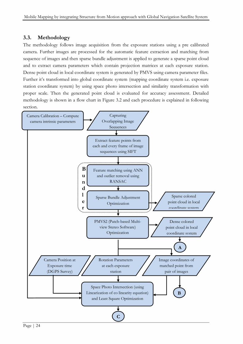
3.3. Methodology
The methodology follows image acquisition from the exposure stations using a pre calibrated
camera. Further images are processed for the automatic feature extraction and matching from
sequence of images and then sparse bundle adjustment is applied to generate a sparse point cloud
and to extract camera parameters which contain projection matrices at each exposure station.
Dense point cloud in local coordinate system is generated by PMVS using camera parameter files.
Further it‟s transformed into global coordinate system (mapping coordinate system i.e. exposure
station coordinate system) by using space photo intersection and similarity transformation with
proper scale. Then the generated point cloud is evaluated for accuracy assessment. Detailed
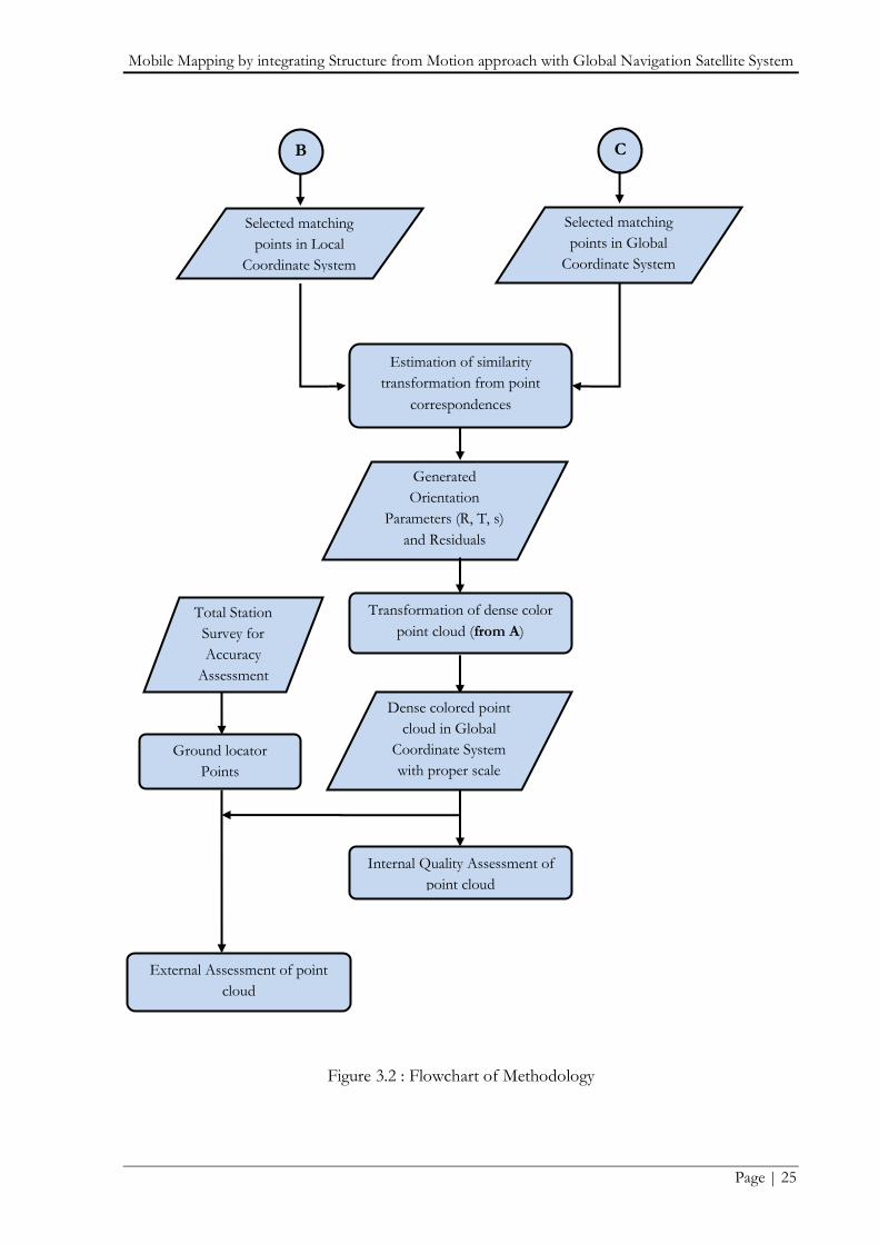
methodology is shown in a flow chart in Figure 3.2 and each procedure is explained in following
section.
B
u n
d l e r
Camera Calibration – Compute
camera intrinsic parameters
Capturing
Overlapping Image
Sequences
Extract feature points from
each and every frame of image
sequences using SIFT
Feature matching using ANN
and outlier removal using
RANSAC
Sparse Bundle Adjustment
Optimization
PMVS2 (Patch-based Multi-
view Stereo Software)
Optimization
Sparse colored
point cloud in local
coordinate system
Dense colored
point cloud in local
coordinate system
Space Photo Intersection (using
Linearization of co linearity equation)
and Least Square Optimization
Camera Position at
Exposure time
(DGPS Survey)
C
A
B
Rotation Parameters
at each exposure
station
)
Image coordinates of
matched point from
pair of images
)
Mobile Mapping by integrating Structure from Motion approach with Global Navigation Satellite System
Page | 25
Figure 3.2 : Flowchart of Methodology
B
Selected matching
points in Local
Coordinate System
C
Selected matching
points in Global
Coordinate System
Estimation of similarity
transformation from point
correspondences
Generated
Orientation
Parameters (R, T, s)
and Residuals
Transformation of dense color
point cloud (from A)
Total Station
Survey for
Accuracy
Assessment
Internal Quality Assessment of
point cloud
External Assessment of point
cloud
Dense colored point
cloud in Global
Coordinate System
with proper scale
Ground locator
Points

Mobile Mapping by integrating Structure from Motion approach with Global Navigation Satellite System
Page | 26
3.3.1. Camera Calibration
Mainly two types of digital cameras are available. One is metric and another one is non metric
camera. Metric cameras are designed particularly for photogrammetry purpose, constructed so
that the geometric distortion of photograph is as small as possible and the camera characteristics
do not change from image to image. Thus metric cameras have precise and stable known internal
geometries, very low lens distortions and which are very expensive devices. A non-metric camera
has to be calibrated for accurate data extraction. Over a period of time calibration data should be
validated carefully before subsequent photogrammetric purpose (Wackrow et al., 2007). Camera
Calibration is done by using PhotoModeler Scanner software‟s automatic calibration module.
This calibration is based on space photo resection method. Automatic camera calibration is based
on collinearity equations, taking automatic image point coordinates from predefined grid, and
estimating intrinsic and external orientation parameters of the camera, distortion factor and other
additional elements (Weizheng et al., 2010). It estimates the interior orientation parameters: focal
length, principal point and lens distortion parameter. Camera calibration experiments and results
are shown in section 4.1 which are used in data planning and space photo intersection process.
3.3.2. Planning for Data Acquisition
The general guidance for terrestrial photography are described in the ISPRS (2010) close range
working V/6 report. As per this report the following are few suggestions for terrestrial
photography. It‟s necessary to visit the site, take various test photos, estimate time required for
preparing, making field notes to study prior to planning. It‟s necessary to look over all possible
working conditions & other site specifics: visibility, weather, equipments, sun/shadows, safety
regulations & legal responsibilities. The quality of the imagery will greatly determine the quality of
the output (data). Therefore, photographic skills should be developed to take consistently sharp
photos in all conditions, for clear and crisp photos which are suitable for photogrammetric use.
The following points should be considered for acquiring the photo.
Use the sharpest aperture setting for your lens (often f/8).
Keep the lens fixed on infinite focus.
Use the fastest shutter speed.
It should be increase the ISO if additional sensitivity is needed.
Use a standard tripod with centering and leveling facility.
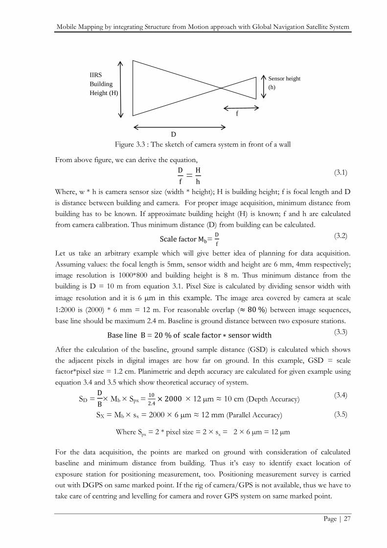
Figure 3.3 shows the sketch of camera system in front of the wall. Before starting the image
acquisition, minimum distance from building, scale, and baseline needs to be calculated for
proper image acquisition.
Mobile Mapping by integrating Structure from Motion approach with Global Navigation Satellite System
Page | 27
Figure 3.3 : The sketch of camera system in front of a wall
From above figure, we can derive the equation,
D
f =
H
h (3.1)
Where, w * h is camera sensor size (width * height); H is building height; f is focal length and D
is distance between building and camera. For proper image acquisition, minimum distance from
building has to be known. If approximate building height (H) is known; f and h are calculated
from camera calibration. Thus minimum distance (D) from building can be calculated.
Scale factor Mb= D
f (3.2)
Let us take an arbitrary example which will give better idea of planning for data acquisition.
Assuming values: the focal length is 5mm, sensor width and height are 6 mm, 4mm respectively;
image resolution is 1000*800 and building height is 8 m. Thus minimum distance from the
building is D = 10 m from equation 3.1. Pixel Size is calculated by dividing sensor width with
image resolution and it is 6 µm in this example. The image area covered by camera at scale
1:2000 is (2000) * 6 mm = 12 m. For reasonable overlap (≈ 80 %) between image sequences,
base line should be maximum 2.4 m. Baseline is ground distance between two exposure stations.
Base line B = 20 % of scale factor ∗ sensor width (3.3)
After the calculation of the baseline, ground sample distance (GSD) is calculated which shows
the adjacent pixels in digital images are how far on ground. In this example, GSD = scale
factor*pixel size = 1.2 cm. Planimetric and depth accuracy are calculated for given example using
equation 3.4 and 3.5 which show theoretical accuracy of system.
SD = D
B× Mb × Spx =
10
2.4× 2000 × 12 µm ≈ 10 cm (Depth Accuracy)
(3.4)
SX = Mb × sx = 2000 × 6 µm ≈ 12 mm (Parallel Accuracy) (3.5)
Where Spx = 2 * pixel size = 2 × sx = 2 × 6 µm = 12 µm
For the data acquisition, the points are marked on ground with consideration of calculated
baseline and minimum distance from building. Thus it‟s easy to identify exact location of
exposure station for positioning measurement, too. Positioning measurement survey is carried
out with DGPS on same marked point. If the rig of camera/GPS is not available, thus we have to
take care of centring and levelling for camera and rover GPS system on same marked point.
f
D
IIRS
Building
Height (H)
Sensor height
(h)
Mobile Mapping by integrating Structure from Motion approach with Global Navigation Satellite System
Page | 28
3.3.3. Features Extraction After the acquisition of images, SIFT is used to extract key features from images. As presented in
section 2.2, SIFT is a most popular features extractor from images. Lowe (1999)‟s SIFT is written
in C/C++. This key-points extractor is available in the form of compiled binary files that can be
run under Linux or Windows environment. This SIFT version takes only gray-scale image of size
1800*1800 pixels or smaller.
3.3.4. Bundler
Snavely (2010) developed an efficient open source software Bundler, in which structure from
motion system is used to generate sparse point clouds. Bundler includes the binary distribution of
the Lourakis et al. (2009)‟s Sparse Bundle Adjustment (SBA), as well as a number of other utilities
and executables. Features matching and outlier removals libraries (ANN and RANSAC) are also
included in this package. Complete package of Snavely (2010)‟s bundler is used to generate sparse
point clouds with exposure station positions and orientation files in its local coordinate system.
After the key point extraction from images, result of SIFT files are used as input for bundler
packages. Following sub section will explain steps involve in bundler.
3.3.4.1. Feature Matching and Outlier Removal
After the key point extraction from images, a presented in section 2.2 ANN (Arya et al., 2010) is
used for feature matching. Features matching have been done between pre and post sequences of
images for each image pair. All images are with approximately 80 % overlap in each pair of
images. ANN is written in ANSI (American National Standards Institute) C++. Thus it‟s needed
C++ compiler which is available in cygwin library databases.
In order to increase the dependability of those matched pair of key-points, as presented in section
2.2., RANSAC algorithm can be implemented to eliminate the wrong matches when the input
datasets has at most 50 % outliers (Fischler et al., 1981). RANSAC algorithm is available in
different languages like Python, MATLAB and C++. Thus as per our conveniences, we will use
any code and apply on our features matched pairs of images to remove outliers.
3.3.4.2. Sparse Bundle Adustment (SBA)
With the help of matched key-points pairs and based on camera multiple view model‟s theory as
presented in section 2.1.4 and 2.3, the relative transformation and orientation of the exposure
station, from which the images are taken can be estimated. SBA package reconstructs the scene
incrementally, a few images at a time as the underlying optimization engine. SBA is generic in the
sense that it gives the user full control over the describing the defination of camera‟s parameters
and 3D structure. It can support any manifestation of the multiple view reconstruction problem
such as partially or fully intrinsically calibrated cameras, arbitrary projective cameras, exterior
orientation estimation from fixed 3D points and refinement of intrinsic parameters (Lourakis et
al., 2009). SBA source files are availbe in C/C++ along with binary files. SBA generates 3D

Mobile Mapping by integrating Structure from Motion approach with Global Navigation Satellite System
Page | 29
colored sparse point clouds and camera exposure position with camera parameter files
(orientation/projection matrices files).
3.3.5. PMVS (Patch Based Multi-view Stereo) Software
PMVS is patch based multi view stereo software to generate 3D dense colored point clouds for
realistic visualization in local coordinate system. It reconstructs the 3D structure of objects with
the camera parameters. The camera parameter file which is generated from Bundler, is used as
one of the inputs for PMVS.
In this method, it only searches around the seed point and in each step it enlarges the search area.
The patch matching optimization is usually done through least square algorithm. This software
automatically ignores non-rigid objects such as pedestrians in front of a building. The software
gives a set of oriented points instead of a polygonal model, where both the 3D coordinate are
estimated at each oriented point (Furukawa et al., 2010). PMVS was written in C++ by Furukawa
et al. (2010). Its complete packages are available in form of source code and compiled binary files.
It also contains camera exterior orientation files and includes a set of matched points with their
positions, color and also from which camera this point is visible. The positions of matched
feature points are in image coordinate system where the origin is the centre of image.
3.3.6. Space Photo Intersection and Least Square Optimization
Space photo intersection is a technique to determine the ground coordinates of points that
appears in overlapping images based on known interior and exterior orientation parameters.
Collinearity equations are used for space photo intersection but since collinearity equations are
not linear, linearization is needed and it‟s done using Taylor series. Mathematics of space photo
intersection for terrestrial photogrammetry is explained below.
The focal length denote as f. Coordinates of the image point a of object point A be 𝑥𝑎 ,
𝑦𝑎 𝑎𝑛𝑑 𝑧𝑎 with respect to 𝑥, 𝑦 image photo coordinate system of which the principal
point (𝑥𝑜, 𝑦𝑜). Image point a having image coordinates 𝑥𝑎 , 𝑦𝑎 𝑎𝑛𝑑 𝑧𝑎 which are in a tilted
photo as that its coordinates rotated into the 𝑥′,𝑦′ 𝑎𝑛𝑑 𝑧′ image space coordinate system which
is parallel to world coordinate system 𝑋,𝑌,𝑍 as shown in below figure. The rotated image
coordinates 𝑥𝑎′ , 𝑦𝑎
′ , 𝑧𝑎′ are related to the measured image coordinates 𝑥𝑎 , 𝑦𝑎 𝑎𝑛𝑑 𝑧𝑎 and three
rotation angles omega ω, phi φ and kappa қ. Coordinates of exposure station be e 𝑋𝐿 ,
𝑌𝐿 𝑎𝑛𝑑 𝑍𝐿 with respect to object world coordinate system 𝑋, 𝑌,𝑍. Coordinates of object point
A be 𝑋𝐴, 𝑌𝐴 𝑎𝑛𝑑 𝑍𝐴 with respect to world coordinate system 𝑋, 𝑌,𝑍. R and T denotes as
rotation and translation matrices respectively. R is a function of rotation angles ω,φ, қ around to
𝑥 ′ , 𝑦′ 𝑎𝑛𝑑 𝑧′ respectively.
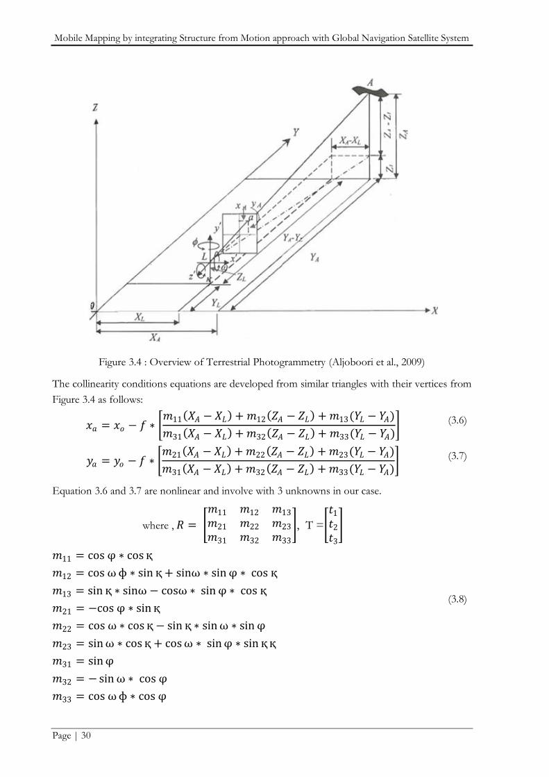
Mobile Mapping by integrating Structure from Motion approach with Global Navigation Satellite System
Page | 30
Figure 3.4 : Overview of Terrestrial Photogrammetry (Aljoboori et al., 2009)
The collinearity conditions equations are developed from similar triangles with their vertices from
Figure 3.4 as follows:
𝑥𝑎 = 𝑥𝑜 − 𝑓 ∗ 𝑚11 𝑋𝐴 − 𝑋𝐿 + 𝑚12 𝑍𝐴 − 𝑍𝐿 + 𝑚13(𝑌𝐿 − 𝑌𝐴)
𝑚31 𝑋𝐴 − 𝑋𝐿 + 𝑚32 𝑍𝐴 − 𝑍𝐿 + 𝑚33(𝑌𝐿 − 𝑌𝐴) (3.6)
𝑦𝑎 = 𝑦𝑜 − 𝑓 ∗ 𝑚21 𝑋𝐴 − 𝑋𝐿 + 𝑚22 𝑍𝐴 − 𝑍𝐿 + 𝑚23(𝑌𝐿 − 𝑌𝐴)
𝑚31 𝑋𝐴 − 𝑋𝐿 + 𝑚32 𝑍𝐴 − 𝑍𝐿 + 𝑚33(𝑌𝐿 − 𝑌𝐴) (3.7)
Equation 3.6 and 3.7 are nonlinear and involve with 3 unknowns in our case.
where , 𝑅 =
𝑚11 𝑚12 𝑚13
𝑚21 𝑚22 𝑚23
𝑚31 𝑚32 𝑚33
, T =
𝑡1
𝑡2
𝑡3
𝑚11 = cos φ ∗ cos қ
𝑚12 = cos ωɸ ∗ sin қ + sinω ∗ sin φ ∗ cos қ
𝑚13 = sin қ ∗ sinω − cosω ∗ sin φ ∗ cos қ
𝑚21 = −cos φ ∗ sin қ
𝑚22 = cos ω ∗ cos қ − sin қ ∗ sin ω ∗ sin φ
𝑚23 = sin ω ∗ cos қ + cos ω ∗ sin φ ∗ sin ққ
𝑚31 = sin φ
𝑚32 = − sin ω ∗ cos φ
𝑚33 = cos ωɸ ∗ cos φ
(3.8)
Mobile Mapping by integrating Structure from Motion approach with Global Navigation Satellite System
Page | 31
The photo coordinates measurements; as well as calibrated principal points and focal length
parameters are considered as a constant. The nonlinear collinearity equations are linearized by
using Taylor series expansions. For linearizing them, equation 3.6 and 3.7 are re-written as
follows :
F1 = 𝑥𝑎= 𝑥𝑜 −𝑟∗𝑓𝑞
(3.9)
F2=𝑦𝑎= 𝑦𝑜 −𝑠∗𝑓𝑞
(3.10)
where, 𝑞 = 𝑚31 𝑋𝐴 − 𝑋𝐿 + 𝑚32 𝑍𝐴 − 𝑍𝐿 + 𝑚33(𝑌𝐿 − 𝑌𝐴) (3.11)
𝑟 = 𝑚11 𝑋𝐴 − 𝑋𝐿 + 𝑚12 𝑍𝐴 − 𝑍𝐿 + 𝑚13(𝑌𝐿 − 𝑌𝐴) (3.12)
𝑠 = 𝑚21 𝑋𝐴 − 𝑋𝐿 + 𝑚22 𝑍𝐴 − 𝑍𝐿 + 𝑚23(𝑌𝐿 − 𝑌𝐴) (3.13)
According to Taylor‟s theorem, equation 3.9 and 3.10 may be expressed in linearized form by
taking partial derivative with respect to all unknowns in general case:
(𝐹1)0 + 𝜕𝐹1
𝜕𝑥
0 𝑑𝑥 +
𝜕𝐹1
𝜕𝜔
0 𝑑𝜔 +
𝜕𝐹1
𝜕𝜙
0
𝑑𝜙 + 𝜕𝐹1
𝜕𝜅
0 𝑑𝜅 +
𝜕𝐹1
𝜕𝑋𝐿
0
𝑑𝑋𝐿
+ 𝜕𝐹1
𝜕𝑍𝐿
0
𝑑𝑍𝐿 + 𝜕𝐹1
𝜕𝑌𝐿
0
𝑑𝑌𝐿 + 𝜕𝐹1
𝜕𝑋
0 𝑑𝑋 +
𝜕𝐹1
𝜕𝑍
0 𝑑𝑍
+ 𝜕𝐹1
𝜕𝑌
0 𝑑𝑌 = 𝑥𝑎
(3.14)
(𝐹2)0 + 𝜕𝐹2
𝜕𝑦
0
𝑑𝑦 + 𝜕𝐹2
𝜕𝜔
0 𝑑𝜔 +
𝜕𝐹2
𝜕𝜙
0
𝑑𝜙 + 𝜕𝐹2
𝜕𝜅
0 𝑑𝜅 +
𝜕𝐹2
𝜕𝑋𝐿
0
𝑑𝑋𝐿
+ 𝜕𝐹2
𝜕𝑍𝐿
0
𝑑𝑍𝐿 + 𝜕𝐹2
𝜕𝑌𝐿
0
𝑑𝑌𝐿 + 𝜕𝐹2
𝜕𝑋
0 𝑑𝑋 +
𝜕𝐹2
𝜕𝑍
0 𝑑𝑍
+ 𝜕𝐹2
𝜕𝑌
0 𝑑𝑌 = 𝑦𝑎
(3.15)
The following is simplified form of equation 3.14 and 3.15:
𝑉𝑥 = 𝑏11𝑑𝜔 + 𝑏12 𝑑𝜙 + 𝑏13𝑑𝜅 − 𝑏14 𝑑𝑋𝐿 − 𝑏15𝑑𝑍𝐿 + 𝑏16𝑑𝑌𝐿 + 𝑏14𝑑𝑋
+ 𝑏15𝑑𝑍 − 𝑏16𝑑𝑌 + 𝐽 (3.16)
𝑉𝑦 = 𝑏21𝑑𝜔 + 𝑏22 𝑑𝜙 + 𝑏23𝑑𝜅 − 𝑏24 𝑑𝑋𝐿 − 𝑏25𝑑𝑍𝐿 + 𝑏26𝑑𝑌𝐿 + 𝑏24𝑑𝑋
+ 𝑏25𝑑𝑍 − 𝑏26𝑑𝑌 + 𝐾
(3.17)
In equations 3.16 and 3.17, 𝐽 = 𝑥𝑎 − 𝐹1 and 𝐾 = 𝑦𝑎 − 𝐹2 and “b” are the coefficient equal
to the partial derivatives with respect to all unknowns. In these coefficients Δ𝑋 = 𝑋𝐴 −
𝑋𝐿 ,Δ𝑌 = 𝑌𝐴 − 𝑌𝐿 𝑎𝑛𝑑 Δ𝑍 = 𝑍𝐴 − 𝑍𝐿

Mobile Mapping by integrating Structure from Motion approach with Global Navigation Satellite System
Page | 32
Equation 3.9 and 3.10 are written for each stereo point for two images. The above all equations
contain unknowns, the number will vary with own problem. In the present work the unknowns
are three 𝑋𝐴, 𝑌𝐴 𝑎𝑛𝑑 𝑍𝐴 . We have to find the value of “b” with respect to 𝑋𝐴, 𝑌𝐴 𝑎𝑛𝑑 𝑍𝐴 as
shown in equation 3.18 and 3.19. Thus in our case matrix b consists of
𝑏14 , 𝑏15 , 𝑏16 , 𝑏24 , 𝑏25 , 𝑏26 𝑎 If the number of equation are equal to or greater than the
unknowns, a solution is possible.
𝑉𝑥 = 𝑏14𝑑𝑋 + 𝑏15𝑑𝑍 − 𝑏16𝑑𝑌 + 𝐽 (3.18)
𝑉𝑦 = 𝑏24𝑑𝑋 + 𝑏25𝑑𝑍 − 𝑏26𝑑𝑌 + 𝐾 (3.19)
To solve this problem, system of collinearity equation 3.18 and 3.19 are expressed in matrix form
as
𝐴𝑚𝑛 ∗ 𝑋𝑛
1 = 𝐿𝑚1 + 𝑉𝑚
1 (3.20)
In the equation 3.20, m is the number of equations and n is the number of unknowns; 𝐴𝑚𝑛 is the
matrix of b‟s coefficients of unknowns; 𝑉𝑚1 is the matrix of residual errors in measure x and y
photo coordinates; 𝑋𝑛1 is the matrix of unknown correction to the initial approximation and 𝐿𝑚
1
is the matrix of constant term J and K. If the number of unknowns are less than the number of
equations, then the least square solution is used to find the probable value of known by using
following matrix equation (Wolf et al., 2004),
𝑋 = (𝐴𝑇𝐴)−1 ∗ (𝐴𝑇 𝐿) (3.21)
The matrix X shows the most probable values of our unknowns. A is shown the b matrix and L
consists of initial constant values.
To start least square optimization, initial approximations are needed for unknowns and it‟s usually
considered by making certain assumptions like vertical photography (Aljoboori et al., 2009; Wolf
et al., 2004).
In our case, initial approximation values are (Aljoboori et al., 2009):
𝑋𝐴 = 𝑌𝐴 ∗ 𝑥𝑙
𝑓
(3.22)
𝑌𝐴 = 𝐵 ∗ 𝑓
𝑝
(3.23)
𝑍𝐴 = 𝑌𝐴 ∗ 𝑦𝑙
𝑓 (3.24)
In Equation 3.22, 3.23 and 3.24, 𝐵 is baseline; p is parallax (𝑥𝑙 − 𝑥𝑟 ). (𝑥𝑙,𝑦𝑙) and (𝑥𝑟,𝑦𝑟) are
image points in left and right images. To solve the equation 3.21 and to find out 𝑋𝐴, 𝑌𝐴 𝑎𝑛𝑑 𝑍𝐴 ,
the quantities that are determined are correction of the initial approximation as given in equation
3.22, 3.23 and 3.24. After the first solution, the computed corrections are added to the initial

Mobile Mapping by integrating Structure from Motion approach with Global Navigation Satellite System
Page | 33
approximations to obtain revised approximations. The procedure is iterated until the magnitude
of correction becomes insignificant (Wolf et al., 2004).
3.3.7. Coordinate Transformation of 3D Point Cloud
As explained in section 3.3.6 (space photo intersection and least square optimization), we need at
least two stereo image pair to calculate ground coordinate of any object point; by giving input as
image point in image coordinate system in both view, exposure stations positions and rotation
parameters of both exposure stations. As described in section 3.3.4 and 3.3.5., camera exterior
orientation parameters files are generated which contain rotation parameters for each exposure
station and position of camera in space coordinate system. We also have a set of files of matched
key-points with their positions in 3D space, from which exposure stations this point is visible.
The positions of matched key-points are in image coordinate system with origin is at the centre
of image. As mentioned in methodology section 3.3.1 and 3.3.2, interior orientation parameters
are computed and DGPS points of exposure stations are acquired. All, these parameters are
applied in space photo intersection technique.
Let us take illustration of arbitrary images/exposure stations 4th and 5th to understand whole
system theoretically. Camera rotation parameters are identified for both exposure stations from
generated files from software and DGPS points have already been measured for that exposure
stations. The position of matched key-points can be easily extracted which is visible in both
images from the generated feature matching files. All parameters values are applied in space
photo intersection technique to find out 3D position of that particular matched point. As
unknowns are three here, at least three equations are needed in space photo intersection to
calculate 3D ground coordinates of any point. In the present study, total four collinearity
equations (2 equation of no.4 image and 2 equation of no.5 image) for one particular match point
are considered. Further, 3D coordinates in global coordinate system of a image point can be
computed by applying least square adjustment on linearization of collinearity equations‟ matrices
as presented in section 3.3.6. Global coordinate system of that matched key-point is same as
exposure station coordinate system. Each matched point can be converted into global coordinate
system by applying these same steps but it‟s time consuming procedure. Instead of these, we can
apply point based similarity transformation algorithm. In this algorithm, the 3D similarity
transformation parameters between the two dataset can be estimated based upon point to point
correspondence; and more details will be explained in next section.
3.3.7.1. Point based Similarity Transformation
Point based Similarity Transformation is the closed-form of solution using least square problem
of 3 or more points (Horn, 1987). There are at least 3 well distributed matched key-points that
must be converted into global coordinate system using space photo intersection to use this
“SimilarityFromPoints” algorithm on whole 3D point cloud. “SimilarityFromPoints” algorithm
estimates 3D similarity transformation parameters between two sets of corresponding points by
minimizing the distances between the points as calculated from equation 3.25. These

Mobile Mapping by integrating Structure from Motion approach with Global Navigation Satellite System
Page | 34
transformation parameters are applied on whole 3D colored point cloud to generate geo-
referenced point cloud with proper scale.
𝑋𝐺𝑙𝑜𝑏𝑎𝑙𝑖
𝑌𝐺𝑙𝑜𝑏𝑎𝑙𝑖
𝑍𝐺𝑙𝑜𝑏𝑎𝑙𝑖
= 𝑠 ∗ 𝑅
𝑋𝑙𝑜𝑐𝑎𝑙𝑖
𝑌𝑙𝑜𝑐𝑎𝑙𝑖
𝑍𝑙𝑜𝑐𝑎𝑙𝑖
+
𝑇𝑥𝑇𝑦𝑇𝑧
(3.25)
Where,
( 𝑋𝑙𝑜𝑐𝑎𝑙𝑖 , 𝑌𝑙𝑜𝑐𝑎𝑙
𝑖 , 𝑍𝑙𝑜𝑐𝑎𝑙𝑖 ) is the coordinate of ith point in local coordinate system
( 𝑋𝐺𝑙𝑜𝑏𝑎𝑙𝑖 ,𝑌𝐺𝑙𝑜𝑏𝑎𝑙
𝑖 , 𝑍𝐺𝑙𝑜𝑏𝑎𝑙𝑖 ) is the coordinate of ith point in global/mapping coordinate system
s is a scale factor; R is a rotation matrix.
𝑇𝑥,𝑇𝑦, 𝑇𝑧 translation vector between two coordinate system.
3.3.8. Accuracy Assessment of 3D Point Cloud
There are several quantitative aspects to be considered including accuracy of individual points,
gaps or occlusion and point density. The main sources of errors appear from camera orientation
and resolution of images. Environmental factor and object properties can also be contribute to
total error budget. The quantitative analysis of point cloud can be assessed by two different
perceptions as internal and external accuracy assessment.
For internal assessment, sample planes are selected from the point cloud and it is used to fit the
selected points to one reference plane. The principal component analysis (PCA) is applied to
determine reference plane parameters. The principal components are the axis of maximum
variation of the data. The robust fitting algorithm is used to obtain the point to the plane
distances. The RANSAC algorithm is used to perform robust plane fitting to adjust the reference
frame. The statistical analysis is done on the points to plane distances. It has been assumed that
the data does not contain gross errors (outliers), the mean indicates systematic errors in the data.
The standard deviation indicates the random errors of the observables and the precision of the
estimated parameters (Khoshelham, 2005; Sande et al., 2010). Different statistical analysis like
Mean, Standard Deviation, Minimum Distance, Maximum Distance, Median Distance, 25th
percentile and 75th percentile of the random errors of the point cloud can be done.
In external assessment, it is evaluated by comparing generated point cloud with highly dense
point cloud like laser point cloud. It can be done by considering corresponding lines and
corresponding planes of highly dense point cloud as a reference to make comparison with
generated point cloud using points to plane distances. If the Laser point cloud or highly dense
point cloud is not available, ground truth can be done by using Total Station. Then Locators
measurement survey has been carried out. Then we can compare the accuracy in easting, nothing
and height with generated point cloud.

Mobile Mapping by integrating Structure from Motion approach with Global Navigation Satellite System
Page | 35
4. RESULTS AND EVALUATION
As explained in the methodology, camera calibration was performed to generate IOPs (intrinsic
orientation parameters) which will be used in the further steps. The image acquisition for
sequence of images and the exposure station position measurement were carried out as per
section 3.3.2 of data planning. Then it was processed for feature extraction and matching
between sequences of images as discussed in 3.3.3 and 3.3.4. Bundle adjustment was applied on it
to generate sparse point cloud and camera parameter files as discussed in section 3.3.4.2.
Generated camera parameter file was used in patch based multi view stereo software to generate
dense 3D point cloud. Feature matching file contains all the matched points along with their
positions in 3D space, from which exposure stations this point is visible. Then it was converted
into global coordinate system with the use of space photo intersection and the similarity form
point correspondences algorithm. Accuracy assessments were carried out on generated point
cloud. Each experiment step will be described in the following section.
4.1. Intrinsic Parameters of Camera
Camera Calibration was done by using PhotoModeler Scanner software. A Nikon D80 SLR
(single lens reflex) digital camera was used here. It is a non-metric camera and has to be calibrated
for accurate data extraction. Figure 4.1 shows the PhotoModelerScanner (2013)‟s camera
calibration sheet (36 inch x 36 inch) which has 140 grid points and 4 control points. As per
PhotoModelerScanner (2013)‟s manual for camera calibration, it needs minimum 6 photographs
from different angle around the calibration sheet covering 80 % of image area. B/W image is
more preferable than color image. Camera should be mounted on the tripod for better calibration
result. In the present study, B/W photographs with 8 different angles have been taken on
physical focal length of 18 mm, imported into the camera calibration module and processed
automatically. The software estimates the interior orientation parameters (IOP): camera's focal
length (f), distortion parameters (decentring/tangential: P1, P2 and radial: K1, K2), format aspect
ratio, and principal point (xo, yo). The resulting calibration data file can be saved on disk for use in
other projects. Estimated IOP are shown in Table 4.1.
Figure 4.1 : Camera Calibration Sheet

Mobile Mapping by integrating Structure from Motion approach with Global Navigation Satellite System
Page | 36
Table 4.1 : Intrinsic Parameters of Camera and Accuracy of Calibration
Parameters Values
f (focal length) 18.494 mm
x,y (location of principal point sensor) 12.245 mm, 8.063 mm
w,h (size of CCD sensor) 23.973 mm, 16.066 mm
K1,K2
(radial distortion function coefficients)
4.856e-004 and -7.632e-007
P1,P2
(decentring distortion function coefficients)
-1.170e-005 and 2.375e-005
Largest point Marking Residual 0.491 pixels
Overall point Marking RMSE 0.126 pixels
Final Total error 1.051 pixels
The maximum point marking residual is 0.491 pixels, overall point marking RMSE is 0.126 pixels
and total error is 1.051 pixels. According to the PhotoModelerScanner (2013) calibration
manuals, maximum point marking residual; and the overall point marking RMSE values should
be lesser than 1.5 pixels and 1 pixel respectively. Thus our values are well within the
recommended values of standard specifications. IOPs have been used in data planning and space
photo intersection process.
4.2. Image Acquistion and DGPS Survey Points
Nikon D80 SLR camera (with physically 18mm focal length) and Leica DGPS 510 was used for
terrestrial image acquisition of the IIRS main building and exposure station position respectively.
For proper image acquisition, minimum distance from building and baseline for same are given
below.
IIRS building Height is H = 11.5 m.
Physical Sensor Size: 23.6 mm * 15.8 mm (w*h).
Sensor Size after calibration: 23.973 mm * 16.066 mm (w*h)
Focal length after calibration f = 18.494 mm
From equation 3.1,
D ≈ 11.5 m
16.066 𝑚𝑚 × 18.494 mm = 13.238 m (minimum distance from building).
In our case, we have taken D ≈ 15 m.
From Equation 3.2,
Scale Mb ≈ 15 m
18.494 mm = 811.
From Equation 3.3,
Baseline B = 811 * 23.973 = 20% of 19.440 ≈ 3.88 m (maximum baseline).
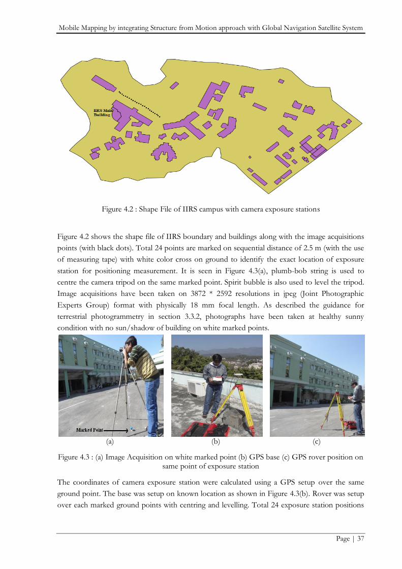
Mobile Mapping by integrating Structure from Motion approach with Global Navigation Satellite System
Page | 37
Figure 4.2 : Shape File of IIRS campus with camera exposure stations
Figure 4.2 shows the shape file of IIRS boundary and buildings along with the image acquisitions
points (with black dots). Total 24 points are marked on sequential distance of 2.5 m (with the use
of measuring tape) with white color cross on ground to identify the exact location of exposure
station for positioning measurement. It is seen in Figure 4.3(a), plumb-bob string is used to
centre the camera tripod on the same marked point. Spirit bubble is also used to level the tripod.
Image acquisitions have been taken on 3872 * 2592 resolutions in jpeg (Joint Photographic
Experts Group) format with physically 18 mm focal length. As described the guidance for
terrestrial photogrammetry in section 3.3.2, photographs have been taken at healthy sunny
condition with no sun/shadow of building on white marked points.
(a)
(b)
(c)
Figure 4.3 : (a) Image Acquisition on white marked point (b) GPS base (c) GPS rover position on same point of exposure station
The coordinates of camera exposure station were calculated using a GPS setup over the same
ground point. The base was setup on known location as shown in Figure 4.3(b). Rover was setup
over each marked ground points with centring and levelling. Total 24 exposure station positions
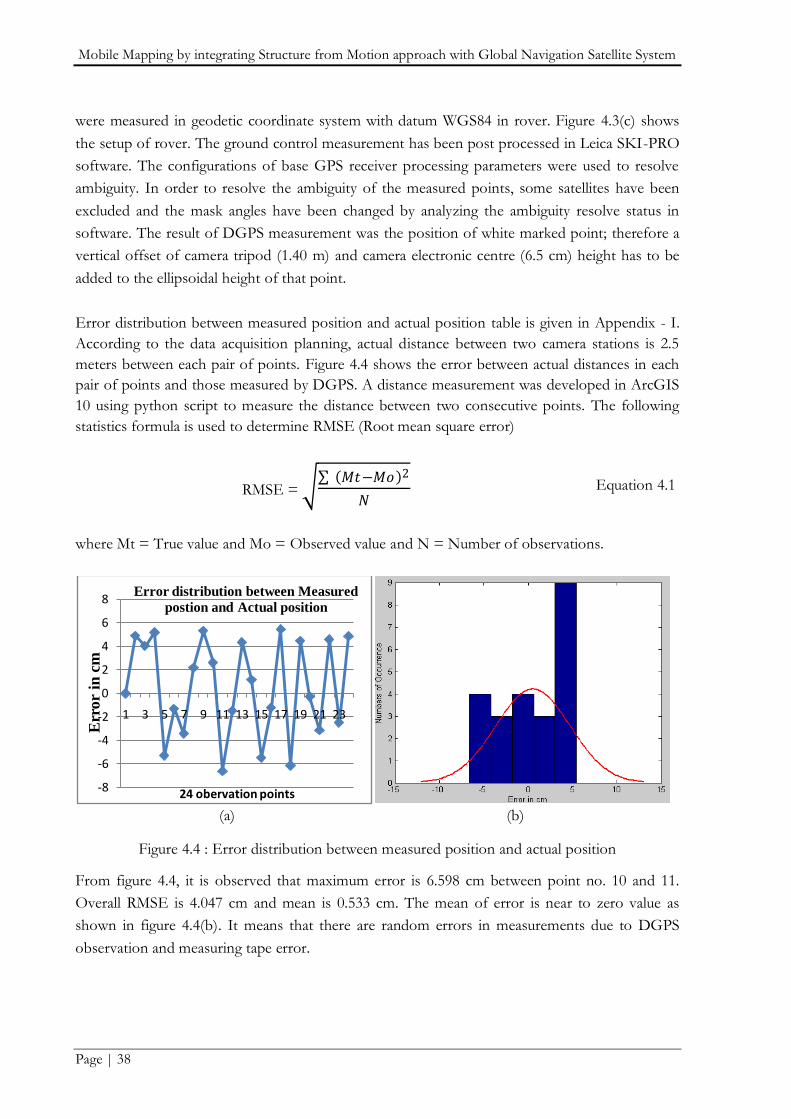
Mobile Mapping by integrating Structure from Motion approach with Global Navigation Satellite System
Page | 38
were measured in geodetic coordinate system with datum WGS84 in rover. Figure 4.3(c) shows
the setup of rover. The ground control measurement has been post processed in Leica SKI-PRO
software. The configurations of base GPS receiver processing parameters were used to resolve
ambiguity. In order to resolve the ambiguity of the measured points, some satellites have been
excluded and the mask angles have been changed by analyzing the ambiguity resolve status in
software. The result of DGPS measurement was the position of white marked point; therefore a
vertical offset of camera tripod (1.40 m) and camera electronic centre (6.5 cm) height has to be
added to the ellipsoidal height of that point.
Error distribution between measured position and actual position table is given in Appendix - I.
According to the data acquisition planning, actual distance between two camera stations is 2.5
meters between each pair of points. Figure 4.4 shows the error between actual distances in each
pair of points and those measured by DGPS. A distance measurement was developed in ArcGIS
10 using python script to measure the distance between two consecutive points. The following
statistics formula is used to determine RMSE (Root mean square error)
RMSE = 𝑀𝑡−𝑀𝑜 2
𝑁 Equation 4.1
where Mt = True value and Mo = Observed value and N = Number of observations.
(a) (b)
Figure 4.4 : Error distribution between measured position and actual position
From figure 4.4, it is observed that maximum error is 6.598 cm between point no. 10 and 11.
Overall RMSE is 4.047 cm and mean is 0.533 cm. The mean of error is near to zero value as
shown in figure 4.4(b). It means that there are random errors in measurements due to DGPS
observation and measuring tape error.
-8
-6
-4
-2
0
2
4
6
8
1 3 5 7 9 11 13 15 17 19 21 23
Err
or
in c
m
24 obervation points
Error distribution between Measured
postion and Actual position

Mobile Mapping by integrating Structure from Motion approach with Global Navigation Satellite System
Page | 39
4.3. Expected Accuracy for Stereo Photogrammetry
The theoretical accuracy is computed and it is expected that in the final oriented image the
accuracy should be within the range. So, it is necessary to calculate planimetric as well as depth
accuracy separately for both types of oriented images. Several aspects of quality are also
considered as accuracy of individual points. The sources of errors mainly appear from camera
orientation and resolution of images. Environmental factor and object properties can also
contribute to total error budget (Khoshelham, 2012). The approximations used are the simplified
normal case, e.g. horizontal/front view, same depth of camera above reference plane (Gerke et
al., 2012).
Expected accuracy for full resolution of images are calculated from Gerke et al. (2012)’s
ITC Lecture Note Series:
As calculated in section 4.1 and 4.2, average depth is D=15 m, f = 18.494 mm, scale is Mb = 811,
sensor size is 23.973 mm * 16.066 mm (w * h) and base length B = 2.5 m
Image resolution ≈ 3872 x 2592
Pixel size, sx ≈ 23.973 mm
3872 pix = 6.20 µm
If it is assumed that the parallax is measured as the difference between two image measurements,
it can be pessimistically assumed (Snavely, 2010).
Spx = 2 x pixel size = 2 × sx = 2 × 6.20 µm = 12.40 µm
SD = D
B× Mb × Spx =
15
2.5× 811 × 12.40 µm ≈ 0.060 m (Depth Accuracy)
SX = Mb × sx = 811 × 6.20 µm ≈ 0.005 m (Parallel Accuracy)
Expected accuracy for re-sampled images are calculated from Gerke et al. (2012)’s ITC
Lecture Note Series:
All the parameters (D, f, Mb , B, w*h) stated as above,
Image resolution ≈ 1704 x 1140
Pixel size, sx ≈ 23.973 mm
1704 pix = 14.069 µm ≈ 14 µm
GSD = scale factor*pixel size = 811*14 µm = 1.135 cm.
Spx = 2 pixel size = 2 × sx = 2 × 14 µm = 28 µm
SD = D
B× Mb × Spx =
15
2.5× 811 × 28 µm = 0.136 m (Depth Accuracy).
SX = Mb×sx= 811 × 14 µm ≈ 0.012 m (Parallel Accuracy).
The above re-sampled theoretical values are considered in accuracy assessment. If the values are
exceed than there may be some blunders or gross errors in data set.
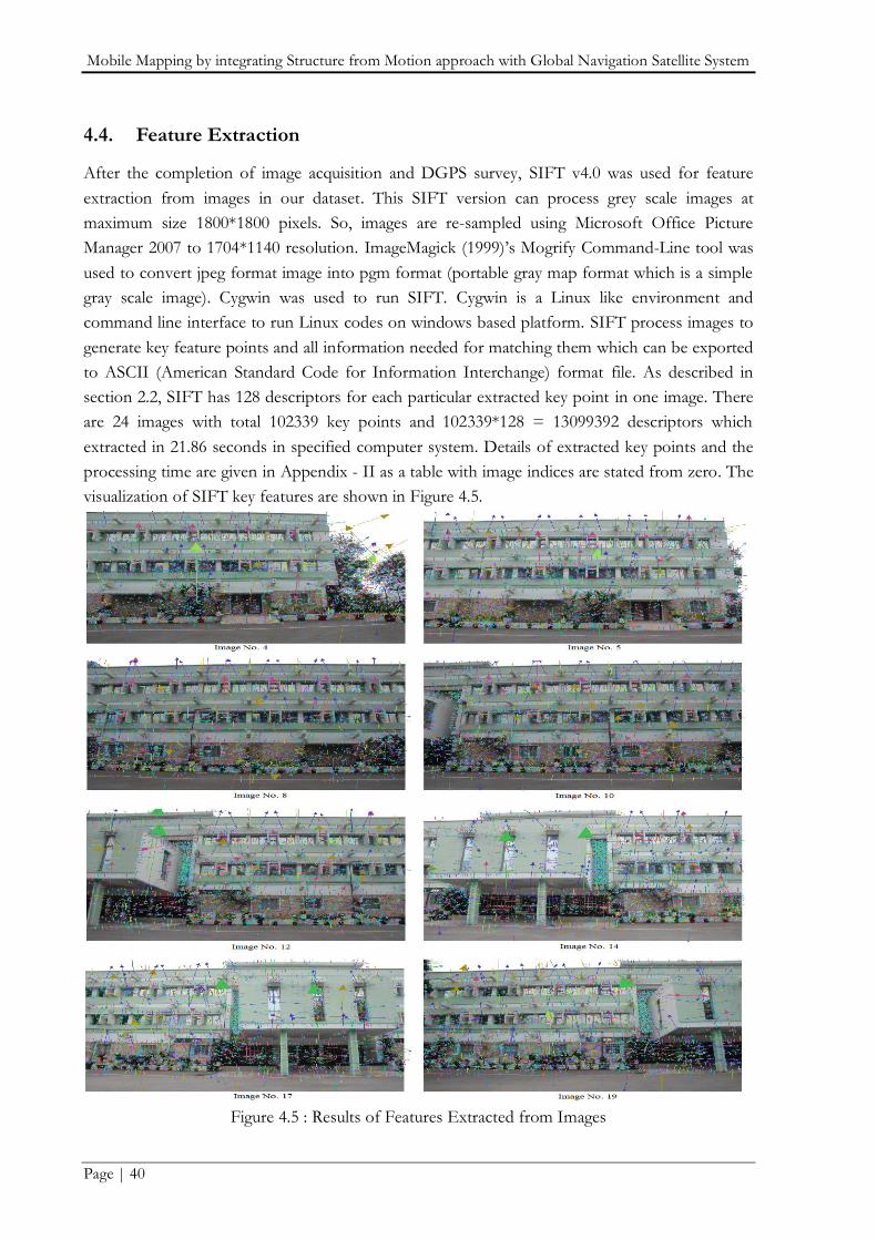
Mobile Mapping by integrating Structure from Motion approach with Global Navigation Satellite System
Page | 40
4.4. Feature Extraction
After the completion of image acquisition and DGPS survey, SIFT v4.0 was used for feature
extraction from images in our dataset. This SIFT version can process grey scale images at
maximum size 1800*1800 pixels. So, images are re-sampled using Microsoft Office Picture
Manager 2007 to 1704*1140 resolution. ImageMagick (1999)‟s Mogrify Command-Line tool was
used to convert jpeg format image into pgm format (portable gray map format which is a simple
gray scale image). Cygwin was used to run SIFT. Cygwin is a Linux like environment and
command line interface to run Linux codes on windows based platform. SIFT process images to
generate key feature points and all information needed for matching them which can be exported
to ASCII (American Standard Code for Information Interchange) format file. As described in
section 2.2, SIFT has 128 descriptors for each particular extracted key point in one image. There
are 24 images with total 102339 key points and 102339*128 = 13099392 descriptors which
extracted in 21.86 seconds in specified computer system. Details of extracted key points and the
processing time are given in Appendix - II as a table with image indices are stated from zero. The
visualization of SIFT key features are shown in Figure 4.5.
Figure 4.5 : Results of Features Extracted from Images
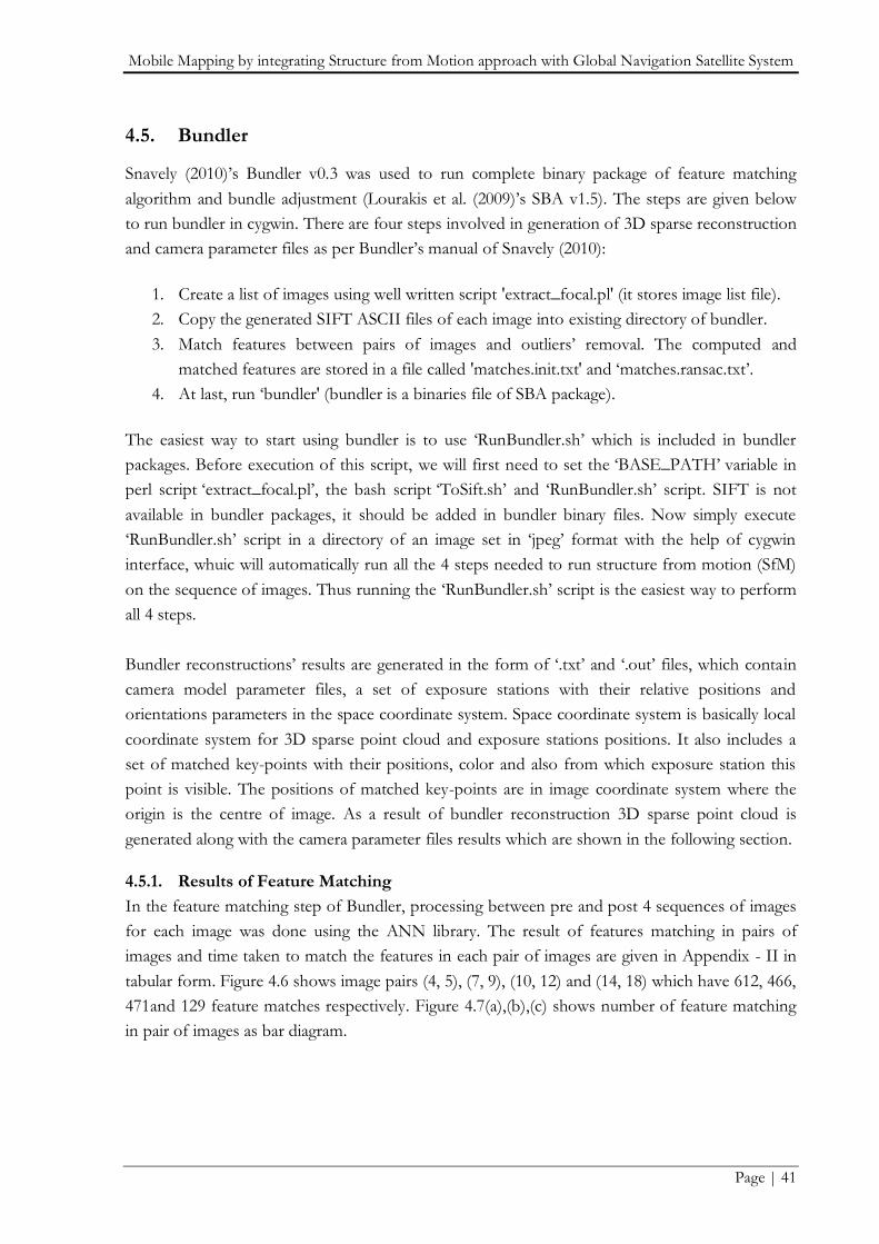
Mobile Mapping by integrating Structure from Motion approach with Global Navigation Satellite System
Page | 41
4.5. Bundler
Snavely (2010)‟s Bundler v0.3 was used to run complete binary package of feature matching
algorithm and bundle adjustment (Lourakis et al. (2009)‟s SBA v1.5). The steps are given below
to run bundler in cygwin. There are four steps involved in generation of 3D sparse reconstruction
and camera parameter files as per Bundler‟s manual of Snavely (2010):
1. Create a list of images using well written script 'extract_focal.pl' (it stores image list file).
2. Copy the generated SIFT ASCII files of each image into existing directory of bundler.
3. Match features between pairs of images and outliers‟ removal. The computed and
matched features are stored in a file called 'matches.init.txt' and „matches.ransac.txt‟.
4. At last, run „bundler' (bundler is a binaries file of SBA package).
The easiest way to start using bundler is to use „RunBundler.sh‟ which is included in bundler
packages. Before execution of this script, we will first need to set the „BASE_PATH‟ variable in
perl script „extract_focal.pl‟, the bash script „ToSift.sh‟ and „RunBundler.sh‟ script. SIFT is not
available in bundler packages, it should be added in bundler binary files. Now simply execute
„RunBundler.sh‟ script in a directory of an image set in „jpeg‟ format with the help of cygwin
interface, whuic will automatically run all the 4 steps needed to run structure from motion (SfM)
on the sequence of images. Thus running the „RunBundler.sh‟ script is the easiest way to perform
all 4 steps.
Bundler reconstructions‟ results are generated in the form of „.txt‟ and „.out‟ files, which contain
camera model parameter files, a set of exposure stations with their relative positions and
orientations parameters in the space coordinate system. Space coordinate system is basically local
coordinate system for 3D sparse point cloud and exposure stations positions. It also includes a
set of matched key-points with their positions, color and also from which exposure station this
point is visible. The positions of matched key-points are in image coordinate system where the
origin is the centre of image. As a result of bundler reconstruction 3D sparse point cloud is
generated along with the camera parameter files results which are shown in the following section.
4.5.1. Results of Feature Matching
In the feature matching step of Bundler, processing between pre and post 4 sequences of images
for each image was done using the ANN library. The result of features matching in pairs of
images and time taken to match the features in each pair of images are given in Appendix - II in
tabular form. Figure 4.6 shows image pairs (4, 5), (7, 9), (10, 12) and (14, 18) which have 612, 466,
471and 129 feature matches respectively. Figure 4.7(a),(b),(c) shows number of feature matching
in pair of images as bar diagram.

Mobile Mapping by integrating Structure from Motion approach with Global Navigation Satellite System
Page | 42
Figure 4.6 : Result of Features Matching in Images
(a)
(b)
408
199
440
170 23
6
551
149 20
5 319
623
195 28
7
307
612
210
261 31
7
718
220 27
3
438
805
268 36
0 465
789
329 39
5 46
6
816
0
200
400
600
800
1000
0,1
0,2
1,2
0,3
1,3
2,3
0,4
1,4
2,4
3,4
1,5
2,5
3,5
4,5
2,6
3,6
4,6
5,6
3,7
4,7
5,7
6,7
4,8
5,8
6,8
7,8
5,9
6,9
7,9
8,9N
um
ber
of
Mta
ch
ing
Matching between image pairs
Number of feature matches in pair of images
386
409 52
6
925
331 43
9 553
873
328
371 47
1
791
264
296 39
1
677
191
243 34
4
746
165
208 29
4
543
132 19
3 297
638
0
200
400
600
800
1000
6,10
7,1
0
8,1
0
9,1
0
7,1
1
8,1
1
9,1
1
10,1
1
8,1
2
9,1
2
10,1
2
11,1
2
9,1
3
10,1
3
11,1
3
12,1
3
10,1
4
11,1
4
12,1
4
13,1
4
11,1
5
12,1
5
13,1
5
14,1
5
12,1
6
13,1
6
14,1
6
15,1
6
Nu
mb
er
of
Mta
ch
ing
Matching between image pairs
Number of feature matches in pair of images

Mobile Mapping by integrating Structure from Motion approach with Global Navigation Satellite System
Page | 43
(c)
Figure 4.7 : (a) (b) (c) Plot of feature matching between pair of images
From above plot, it is clear that matched features between consecutive images are more
compared to other pairings because they have approximately 80 % overlap. It‟s not possible that
all features matching pairs are true; there are lots of outliers between pairs of images which are
shown in Figure 4.6.
4.5.2. Results after Removal of Outliers
In order to increase the reliability of those matched pair of key-points, RANSAC algorithm was
used to eliminate the wrong matches (outliers). The results after outliers‟ removal in features
matching from the pairs of images and time taken to removal of outliers in pairs of images are
given in Appendix - II as a table form. Figure 4.8 shows same pairs of (4, 5), (7, 9), (10, 12) and
(14, 18) images which have 449, 270, 302 and 44 feature matches inliers respectively after removal
of outliers using RANSAC.
Figure 4.8 : Results of Features Matching Images after RANSAC
105
144 23
8
524
129
176 28
6
649
147
203 35
2
892
120 19
3 327
776
131 20
4 349
643
144 20
7 270
503
77 114 19
7
374
0
200
400
600
800
1000
13
,17
14
,17
15
,17
16
,17
14
,18
15
,18
16
,18
17
,18
15
,19
16
,19
17
,19
18
,19
16
,20
17
,20
18
,20
19
,20
17
,21
18
,21
19
,21
20
,21
18
,22
19
,22
20
,22
21
,22
19
,23
20
,23
21
,23
22
,23N
um
ber
of
Mta
ch
ing
Matching between image pairs
Number of feature matches in pair of images
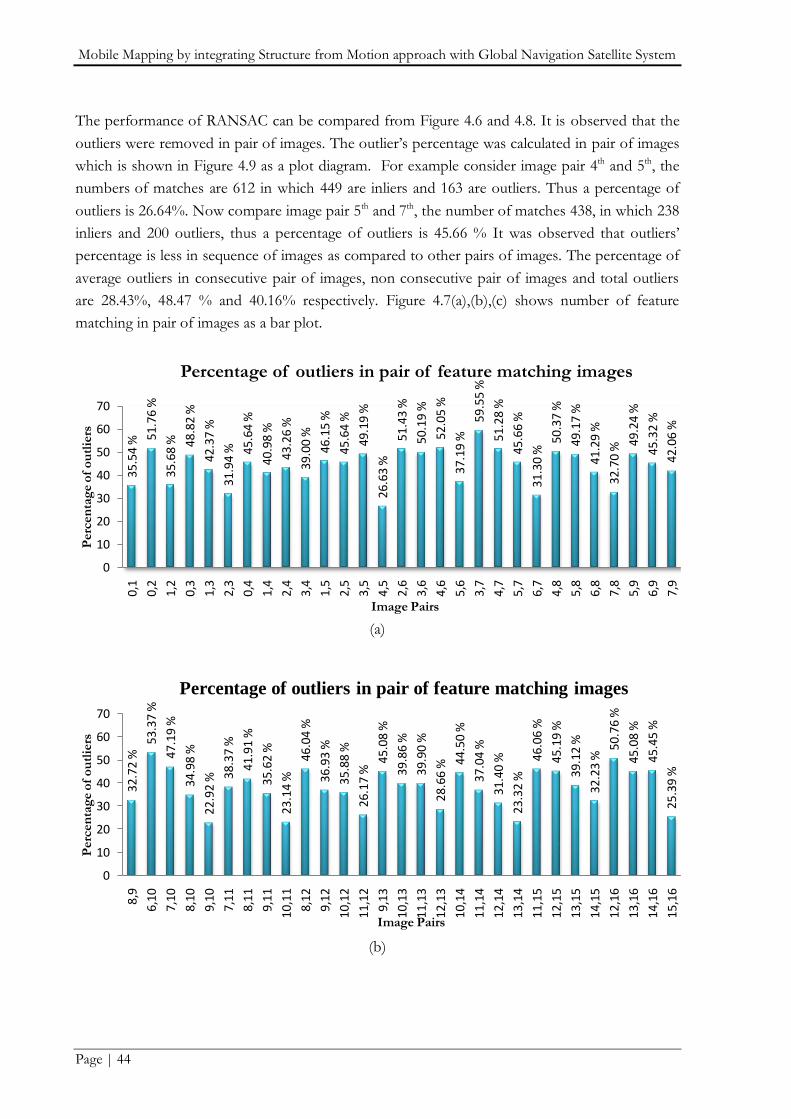
Mobile Mapping by integrating Structure from Motion approach with Global Navigation Satellite System
Page | 44
The performance of RANSAC can be compared from Figure 4.6 and 4.8. It is observed that the
outliers were removed in pair of images. The outlier‟s percentage was calculated in pair of images
which is shown in Figure 4.9 as a plot diagram. For example consider image pair 4th and 5th, the
numbers of matches are 612 in which 449 are inliers and 163 are outliers. Thus a percentage of
outliers is 26.64%. Now compare image pair 5th and 7th, the number of matches 438, in which 238
inliers and 200 outliers, thus a percentage of outliers is 45.66 % It was observed that outliers‟
percentage is less in sequence of images as compared to other pairs of images. The percentage of
average outliers in consecutive pair of images, non consecutive pair of images and total outliers
are 28.43%, 48.47 % and 40.16% respectively. Figure 4.7(a),(b),(c) shows number of feature
matching in pair of images as a bar plot.
(a)
(b)
35.5
4 % 51
.76
%
35.6
8 % 48
.82
%
42.3
7 %
31.9
4 % 45
.64
%
40.9
8 %
43.2
6 %
39.0
0 %
46.1
5 %
45.6
4 %
49.1
9 %
26.6
3 %
51.4
3 %
50.1
9 %
52.0
5 %
37.1
9 %
59.5
5 %
51.2
8 %
45.6
6 %
31.3
0 %
50.3
7 %
49.1
7 %
41.2
9 %
32.7
0 % 49
.24
%
45
.32
%
42.0
6 %
0
10
20
30
40
50
60
70
0,1
0,2
1,2
0,3
1,3
2,3
0,4
1,4
2,4
3,4
1,5
2,5
3,5
4,5
2,6
3,6
4,6
5,6
3,7
4,7
5,7
6,7
4,8
5,8
6,8
7,8
5,9
6,9
7,9
Perc
en
tag
e o
f o
utl
iers
Image Pairs
Percentage of outliers in pair of feature matching images
32.7
2 %
53.3
7 %
47.1
9 %
34.9
8 %
22.
92 % 3
8.3
7 %
41.
91 %
35.6
2 %
23.
14
%
46.0
4 %
36.9
3 %
35.8
8 %
26.
17
%
45.
08 %
39.8
6 %
39.
90 %
28.6
6 % 4
4.50
%
37.0
4 %
31
.40
%
23.
32
%
46.0
6 %
45.1
9 %
39.
12 %
32.2
3 %
50.
76 %
45.
08 %
45.4
5 %
25.3
9 %
0
10
20
30
40
50
60
70
8,9
6,1
0
7,1
0
8,1
0
9,1
0
7,1
1
8,1
1
9,1
1
10,
11
8,1
2
9,12
10,
12
11,
12
9,1
3
10,
13
11,
13
12,
13
10,
14
11,
14
12,
14
13,
14
11,1
5
12,
15
13,
15
14,
15
12,
16
13,
16
14,
16
15,
16
Perc
en
tag
e o
f o
utl
iers
Image Pairs
Percentage of outliers in pair of feature matching images
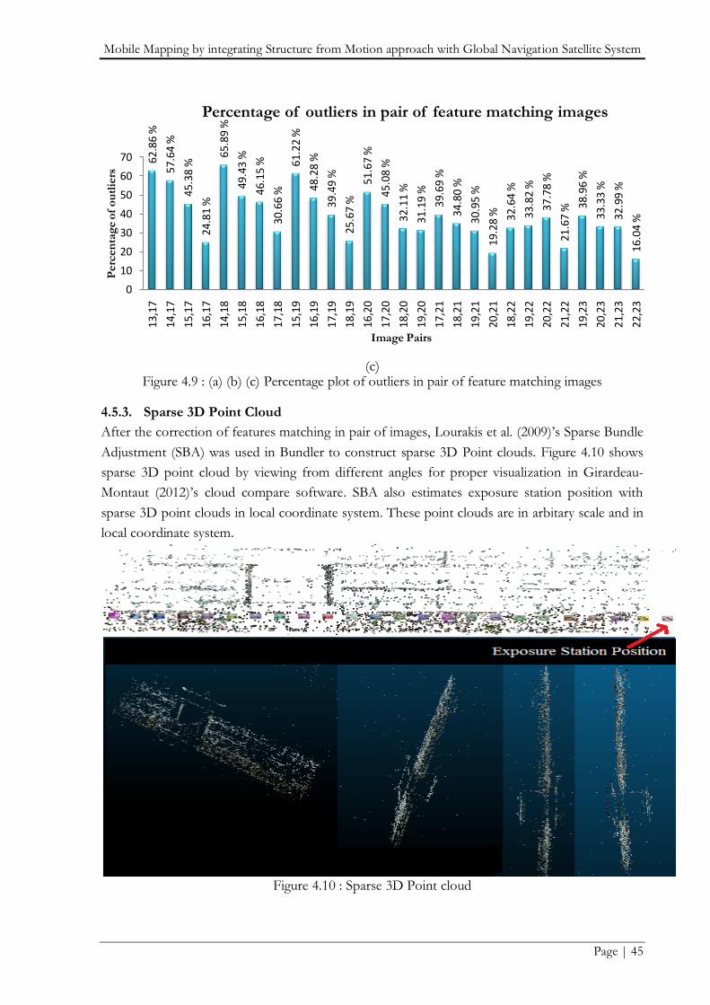
Mobile Mapping by integrating Structure from Motion approach with Global Navigation Satellite System
Page | 45
(c) Figure 4.9 : (a) (b) (c) Percentage plot of outliers in pair of feature matching images
4.5.3. Sparse 3D Point Cloud
After the correction of features matching in pair of images, Lourakis et al. (2009)‟s Sparse Bundle
Adjustment (SBA) was used in Bundler to construct sparse 3D Point clouds. Figure 4.10 shows
sparse 3D point cloud by viewing from different angles for proper visualization in Girardeau-
Montaut (2012)‟s cloud compare software. SBA also estimates exposure station position with
sparse 3D point clouds in local coordinate system. These point clouds are in arbitary scale and in
local coordinate system.
Figure 4.10 : Sparse 3D Point cloud
62.8
6 %
57.6
4 %
45.3
8 %
24.8
1 %
65.8
9 %
49.4
3 %
46.1
5 %
30.6
6 %
61.2
2 %
48.2
8 %
39.4
9 %
25.6
7 %
51.6
7 %
45.0
8 %
32.1
1 %
31.1
9 %
39.6
9 %
34.8
0 %
30.9
5 %
19.2
8 % 32
.64
%
33.8
2 %
37.7
8 %
21.6
7 % 38
.96
%
33.3
3 %
32.9
9 %
16.0
4 %
0
10
20
30
40
50
60
7013
,17
14,1
7
15,1
7
16,1
7
14,1
8
15,1
8
16,1
8
17,1
8
15,1
9
16,1
9
17,1
9
18,1
9
16,2
0
17,2
0
18,2
0
19,2
0
17,2
1
18,2
1
19,2
1
20,2
1
18,2
2
19,2
2
20,2
2
21,2
2
19,2
3
20,2
3
21,2
3
22,2
3
Perc
en
tag
e o
f o
utl
iers
Image Pairs
Percentage of outliers in pair of feature matching images

Mobile Mapping by integrating Structure from Motion approach with Global Navigation Satellite System
Page | 46
3D sparse point cloud is in „.ply‟ format file which is generally known as „polygon file format‟.
The format was specially designed to visualize three dimensional data. Each point entry in „.ply‟
file is in the form of position and color in one line. “Position” is vector showing the 3D position
of the point in space coordinate system. “Color” is a 3D-vector describing the RGB color of the
point. Camera parameter file contains orientation information of each exposure station.
4.6. Results of PMVS (Patch based Multiview Stereo) Software
PMVS v2.0 was used to generate dense point clouds. As shown in Figure 4.10, sparse 3D point
cloud has sparse visualization, in which the particular feature from that point cloud is not
identified easily. Generated camera parameter‟s file of Bundler results are used as one input of
Multi View Stereo (MVS) software as described in 3.3.5. Dense 3D point cloud was generated in
arbitrary coordinate system with arbitrary scale and visualized in cloud compare software as
shown in Figure 4.11. There are three steps to create a 3D dense reconstruction:
1. Check relevant library packages of cygwin as mentioned in Furukawa et al. (2010)‟s
Manual
2. Used bundler camera parameters files but which is in bundler „.out‟ format. Bundler
packages also have a converter („Bundler2PMVS‟) that changes camera parameters from
the Bundler format to the PMVS format and it‟s used as an input in PMVS.
3. And, run „pmvs2' (binaries file of PMVS2) with default settings.
PMVS reconstructions‟ results are generated in „.ply‟, „.patch‟ and „.pset‟ which contain 3D dense
color point cloud, patches reconstruction information (features matching) and 3D locations of
estimated surface normal for all the reconstructed points. 3D colored dense point cloud is
available in „.ply‟ format file. It also contains camera exterior orientation files and includes a set of
matched key-points with their positions, color and also the camera information from which this
point is visible. The positions of matched points are in image coordinate system with the origin at
centre of image. 3D colored dense point cloud results is shown in Figure 4.11. Each 3D point in
the point cloud file has the same format as that of sparse point cloud file.

Mobile Mapping by integrating Structure from Motion approach with Global Navigation Satellite System
Page | 47
Figure 4.11 : Dense 3D Point Cloud
4.7. Coordinate Transformation of 3D Point Cloud
The generated point cloud is in the local coordinate system which needs to be transformed into
global coordinate system. As described in section 3.3.6 and 3.3.7.1, space photo intersection
technique and similarity form points technique respectively was used to transform local
coordinate system of point cloud into global coordinate system and introduce proper scale.
Following sections will explain how it can be achieved.
4.7.1. Feature Matching File
Generated “ply” file contains 3D location of points with their RGB features. Features Matching
file was generated which contains the estimated scene with the information in particular format.
Each point entry has the form (Figure 4.12, highlighted with grey color): “Position” is a vector
describing the 3D position of the point in local coordinate system (see line 2769). “Color” is a 3D
vector describing the RGB color of the point] (see line 2770), “Viewing list” is a list of views the
point is visible in (see line 2771).
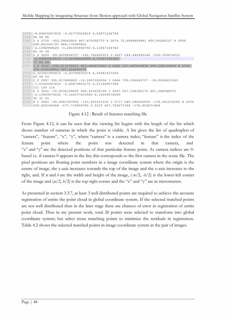
Mobile Mapping by integrating Structure from Motion approach with Global Navigation Satellite System
Page | 48
Figure 4.12 : Result of features matching file
From Figure 4.12, it can be seen that the viewing list begins with the length of the list which
shows number of cameras in which the point is visible. A list gives the list of quadruplets of
“camera”, “feature”, “x”, “y”, where “camera” is a camera index, “feature” is the index of the
feature point where the point was detected in that camera, and
“x” and “y” are the detected positions of that particular feature point. As camera indices are 0-
based i.e. if camera 0 appears in the list; this corresponds to the first camera in the scene file. The
pixel positions are floating point numbers in a image coordinate system where the origin is the
centre of image, the y-axis increases towards the top of the image and the x-axis increases to the
right, and. If w and h are the width and height of the image, (-w/2, -h/2) is the lower-left corner
of the image and (w/2, h/2) is the top-right corner and the “x” and “y” are in micrometers.
As presented in section 3.3.7, at least 3 well distributed points are required to achieve the accurate
registration of entire the point cloud in global coordinate system. If the selected matched points
are not well distributed then in the later stage there are chances of error in registration of entire
point cloud. Thus in my present work, total 20 points were selected to transform into global
coordinate system; but select more matching points to minimize the residuals in registration.
Table 4.2 shows the selected matched points in image coordinate system in the pair of images.

Mobile Mapping by integrating Structure from Motion approach with Global Navigation Satellite System
Page | 49
Image Pairs x1 (μm) y1 (μm) x2 (μm) Y2 (μm) 1,2 519.344726563 214.666259766 468.16027832 192.461853027
2,3 -98.8330688477 491.715026855 224.634399414 476.291717529
3,4 27.2991333008 -163.636535645 298.714599609 -163.885009766
4,5 -365.998687744 -352.016052246 -178.48626709 -372.213500977
5,6 316.130249023 -87.7821655273 567.076782227 -86.1928710938
6,7 273.182495117 413.622833252 517.315795898 387.508422852
8,9 -389.170806885 -357.848022461 -128.394775391 -353.368896484
9,10 -369.320098877 86.2961120605 -205.468933105 86.2473754883 10,11 386.000488281 -262.626647949 644.385620117 -264.055053711
11,12 -71.1900634766 142.962799072 89.5184936523 140.989227295
12,13 258.561035156 -332.664733887 455.059814453 -334.319030762
13,14 -695.419189453 311.699035645 -570.352050781 323.069213867
14,15 -439.026031494 122.651519775 -218.123657227 121.060302734
15,16 385.33261719 334.773345947 607.051513672 338.443969727
16,17 -694.179626465 154.609344482 -490.06237793 156.44342041
17,18 327.739990234 -261.047912598 591.761962891 -261.296142578
18,19 -525.512451172 -353.082702637 -409.156707764 -339.383483887
19,20 230.309204102 -311.684509277 359.709838867 -292.184326172
20,21 679.004638672 -59.5786743164 719.117919922 -48.610534668
22,23 618.182739258 173.346435547 533.997558594 172.550720215
Table 4.2 : Position of matched points in stereo image (image coordinate system)
4.7.2. Rotation Matrix (R) of Exposure Station
Generated camera parameter file consists of the rotation parameter of each exposure station. The
Rotation matrix R is orthogonal, i.e. R-1 = RT.Therefore, we have to check the orthogonality of
the rotation matrix for each exposure station from camera parameter files. Thus by checking the
property of exposure station, we can grant that each exposure station has true rotation matrix. In
our case each exposure station is followed the orthogonality of rotation matrix. Figure 4.13 shows
the snapshot of camera parameter files for exposure station 3 and 4 (highlighted with grey color).
Table 4.3 : Rotation Matrices for exposure station 3 and 4
R3 (Rotation Matrix for exposure station 3)
0.9994 -0.0042 -0.03617
0.0098 0.9878 0.1557
0.0351 -0.1559 0.9871
R4 (Rotation Matrix for exposure station 4)
0.9998 -0.0203 0.0025
0.0197 0.9878 0.1542
-0.0056 -0.1541 0.9880

Mobile Mapping by integrating Structure from Motion approach with Global Navigation Satellite System
Page | 50
Figure 4.13 : Generated camera parameter file
4.7.3. Transformation
As explained in previous sections, we have exposure stations positions (section 4.2), 20 image
points in stereo pairs (section 4.7.1) and rotation matrix (R) of each exposure station (section
4.7.2). As mentioned in section 4.7.1, we have position of all 3D point cloud in local coordinate
system. Table 4.4 shows global coordinate (Cartesian coordinate system) of all 20 points with
correspondences local 3D coordinate system. As presented in section 3.3.6, space photo
intersection with least square adjustment was applied using Al-sadik (2012a)‟s MATLB code with
some modification to suit the present work requirements to convert all 20 points into global
coordinate system. As presented in section 3.3.7.1, point based similarity transformation is
applied on two datasets for 20 points (one dataset contains local coordinate system and other
contains global coordinate system). Khoshelham (2012)‟s MATLAB code was used to calculate
transformation parameters (rotation R, translation T, scale s) and residuals from two dataset.
Then transformation parameters are applied on entire point cloud for geo-referencing and to
produce correct scale in point cloud. The residuals (res) values show the accuracy of model.
Transformation Parameters have 3 translation, 3 rotation and one scale factor thus 7 parameters
are there. To calculate 7 transformation parameters at least 3 measured points are used as shown
in equation 3.25 and other points can be used for accuracy assessment. Figure 4.14 shows the
final scaled colored point cloud in global coordinate system. It‟s showed into UTM projection
with datum WGS84 for proper visualization in cloud compare point picking software. Table 4.5
shows the transformation parameters.
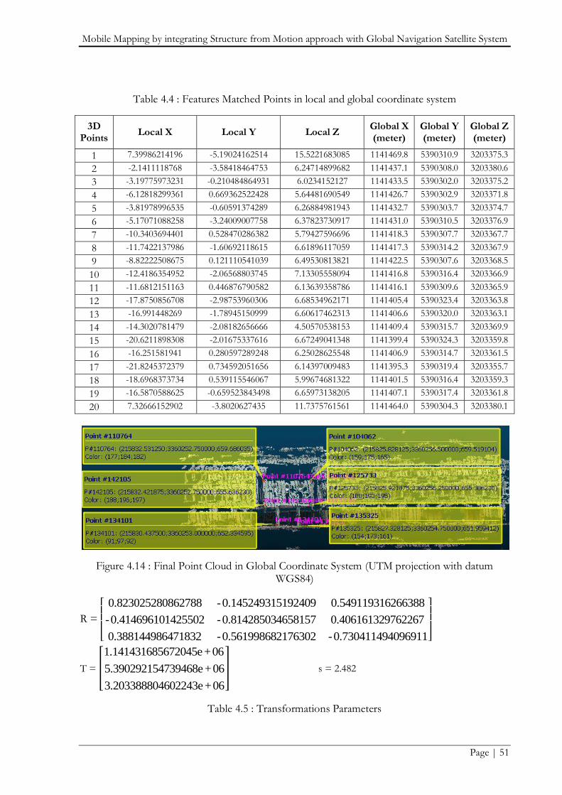
Mobile Mapping by integrating Structure from Motion approach with Global Navigation Satellite System
Page | 51
Table 4.4 : Features Matched Points in local and global coordinate system
3D Points
Local X Local Y Local Z Global X (meter)
Global Y (meter)
Global Z (meter)
1 7.39986214196 -5.19024162514 15.5221683085 1141469.8 5390310.9 3203375.3
2 -2.1411118768 -3.58418464753 6.24714899682 1141437.1 5390308.0 3203380.6
3 -3.19775973231 -0.210484864931 6.0234152127 1141433.5 5390302.0 3203375.2
4 -6.12818299361 0.669362522428 5.64481690549 1141426.7 5390302.9 3203371.8
5 -3.81978996535 -0.60591374289 6.26884981943 1141432.7 5390303.7 3203374.7
6 -5.17071088258 -3.24009007758 6.37823730917 1141431.0 5390310.5 3203376.9
7 -10.3403694401 0.528470286382 5.79427596696 1141418.3 5390307.7 3203367.7
8 -11.7422137986 -1.60692118615 6.61896117059 1141417.3 5390314.2 3203367.9
9 -8.82222508675 0.121110541039 6.49530813821 1141422.5 5390307.6 3203368.5
10 -12.4186354952 -2.06568803745 7.13305558094 1141416.8 5390316.4 3203366.9
11 -11.6812151163 0.446876790582 6.13639358786 1141416.1 5390309.6 3203365.9
12 -17.8750856708 -2.98753960306 6.68534962171 1141405.4 5390323.4 3203363.8
13 -16.991448269 -1.78945150999 6.60617462313 1141406.6 5390320.0 3203363.1
14 -14.3020781479 -2.08182656666 4.50570538153 1141409.4 5390315.7 3203369.9
15 -20.6211898308 -2.01675337616 6.67249041348 1141399.4 5390324.3 3203359.8
16 -16.251581941 0.280597289248 6.25028625548 1141406.9 5390314.7 3203361.5
17 -21.8245372379 0.734592051656 6.14397009483 1141395.3 5390319.4 3203355.7
18 -18.6968373734 0.539115546067 5.99674681322 1141401.5 5390316.4 3203359.3
19 -16.5870588625 -0.659523843498 6.65973138205 1141407.1 5390317.4 3203361.8
20 7.32666152902 -3.8020627435 11.7375761561 1141464.0 5390304.3 3203380.1
Figure 4.14 : Final Point Cloud in Global Coordinate System (UTM projection with datum WGS84)
R =
08627880.82302528 51924090.14524931- 62663880.54911931
14255020.41469610- 46581570.81428503- 97622670.40616132
64718320.38814498 21763020.56199868- 40969110.73041149-
T =
06+5672045e1.14143168
06+4739468e5.39029215
06+4602243e3.20338880
s = 2.482
Table 4.5 : Transformations Parameters

Mobile Mapping by integrating Structure from Motion approach with Global Navigation Satellite System
Page | 52
(a) (b)
Figure 4.15 : (a) Plotting of residuals (b) Probability density function of residuals
From Figure 4.15 (a), it can be seen that the residuals‟ results are in some cm ranges with a
maximum value of residual 17.7 cm. Mean is 3.45 cm and median is 2 cm. It can also be
considered that image capturing method and the resolution of image has effect on the accuracy of
model.
4.8. Accuracy Assessment of Point Cloud
As presented in section 3.3.8, the assessments of point clouds are mainly divided into two
categories: Internal Accuracy Assessment and External Accuracy Assessment.
4.8.1. Internal Assessment of Point Cloud
The main task is to assess the quality of the orientation of the point cloud. There are several
quality aspects to be considered such as accuracy of individual points, point density, gaps or
occlusion etc. Figure 4.16 shows the point cloud of IIRS building using Point Cloud Mapper
(PCM) Software of Vosselman (2012). As presented in section 3.3.8, for internal accuracy
assessment, patches are selected and are fitted into plane; then the points-to-plane distances are
computed. The sample data sets were taken from three different areas as shown in Figure 4.16.
The samples data from corresponding planes were cropped in PCM software and imported into
Khoshelham (2012)‟s MATLAB code and processing was performed. Sample group 1, 2 and 3
have 1205, 2560 and 645 samples respectively. The different statistical analysis (Mean, Standard
Deviation (SD), Minimum Distance, Maximum Distance, Median Distance, 25th percentile and
75th percentile) are also computed to perform this accuracy assessment. Histograms were also
plotted for comparison of each group dataset.
Figure 4.17 (a), 4.18 (a) and 4.19 (a) shows the scattering of samples and the color-bar shows the
scattering of points from the best fitted plane for northing direction (Y). Figure 4.17 (b), 4.18 (b)
and 4.19 (b) shows the outliers with blue color after selecting the reference plane for particular
sample dataset. Figure 4.20 shows the histogram of points-to-plane distance for group 1, 2, and 3.
Figure 4.21 shows the box plot of points-to-plane distance for statistical analysis.
0
0.05
0.1
0.15
0.21 2 3 4 5 6 7 8 9 10 11 12 13 14 15 16 17 18 19 20
Resi
du
als
error in
m
Points
Residuals
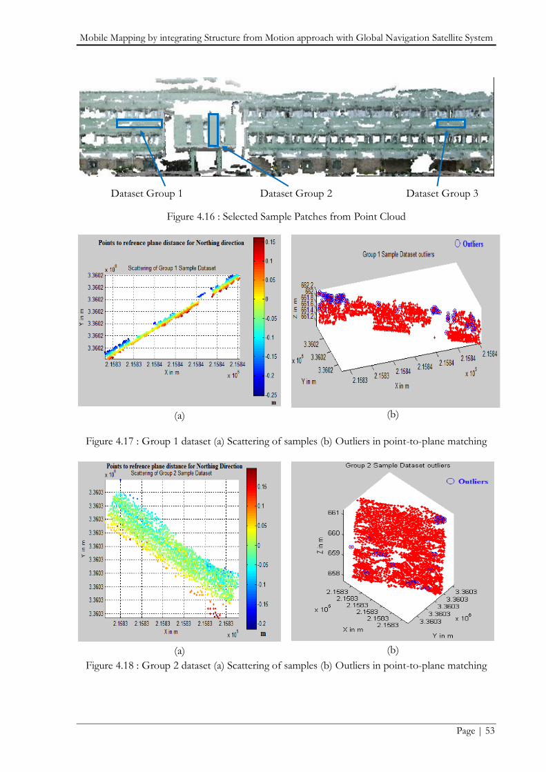
Mobile Mapping by integrating Structure from Motion approach with Global Navigation Satellite System
Page | 53
Dataset Group 1 Dataset Group 2 Dataset Group 3
Figure 4.16 : Selected Sample Patches from Point Cloud
(a) (b)
Figure 4.17 : Group 1 dataset (a) Scattering of samples (b) Outliers in point-to-plane matching
(a)
(b)
Figure 4.18 : Group 2 dataset (a) Scattering of samples (b) Outliers in point-to-plane matching
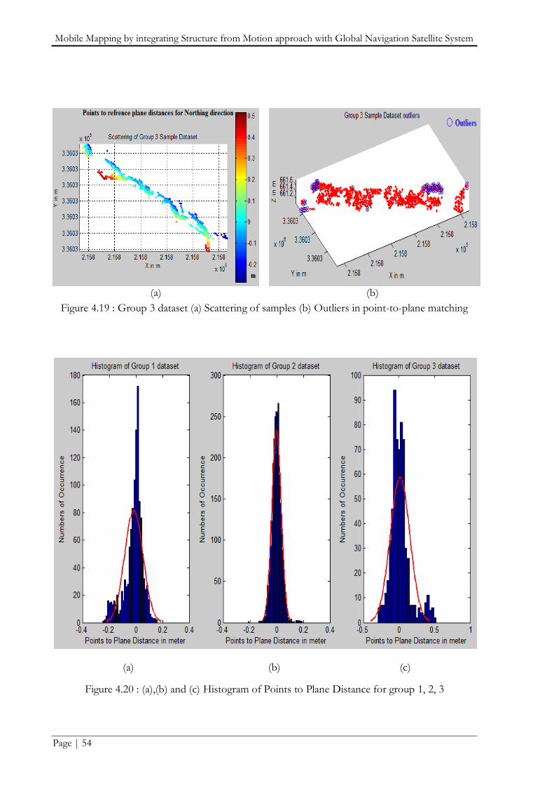
Mobile Mapping by integrating Structure from Motion approach with Global Navigation Satellite System
Page | 54
(a) (b)
Figure 4.19 : Group 3 dataset (a) Scattering of samples (b) Outliers in point-to-plane matching
(a) (b) (c)
Figure 4.20 : (a),(b) and (c) Histogram of Points to Plane Distance for group 1, 2, 3

Mobile Mapping by integrating Structure from Motion approach with Global Navigation Satellite System
Page | 55
Figure 4.21 : Box Plot of Group 1, 2, 3 sample dataset for points-to-plane Distance
Table 4.6 : Internal Statistics for Accuracy Assessment of Point Cloud
Statistics/Dataset Group 1 (m) Group 2 (m) Group 3 (m)
Mean - 0.0152 0 0.0182
Variance 0.0047 0.0012 0.0186
Standard Deviation 0.0685 0.0352 0.1362 Minimum Distance - 0.2530 -0.2134 - 0.2770
Maximum Distance 0.1659 0.1955 0.5114 Median Distance 0 0 0
In Figure 4.21 Boxplot, middle red line shows 50% of data is greater than this value (median).
Bottom blue line shows 25% of data less than this value (Lower Quartile). Top blue line shows
25% of data above than this value (Upper Quartile). Bottom red plus sign shows the outliers
which is less than 1.5 times of lower quartile. Top red plus sign shows the outliers which is more
than 1.5 times of upper quartile. Bottom black line shows least values excluding outliers
(Minimum). Top black line shows greatest value excluding outliers (Maximum).
Figure 4.20 and 4.21 shows that there are two types of distributions in sample dataset. First one is
symmetrical and another one is asymmetrical. Asymmetrical is further classified in negative and
positive skew distribution. Median and quartiles have more advantages than mean and standard
deviation to check outliers. In Figure 4.21, the spacing between the different parts of the box
indicates the degree of dispersion (spread) and skewness in the point cloud data, and identifies
outliers.

Mobile Mapping by integrating Structure from Motion approach with Global Navigation Satellite System
Page | 56
From Figure 4.17 (a), 4.18 (a), 4.19 (a) and Table 4.6, it can be seen that points to plane distance
is in the range of -25.30 cm to 16.59 cm, -21.34 cm to 19.55 cm and -27 cm to 51 cm for group 1,
2 and3 dataset respectively. The 67 % of all observations lie between one standard deviation from
the mean. It is observed that distances are having standard deviation (6.8 cm, 3.5 cm and 13.6
cm) from the Mean (-1.5 cm, 0 and 1.82 cm) in group 1, 2 and 3 respectively. It can be seen from
Figure 4.21, skewness is slightly negative (left skew), symmetric distribution (mean = median) and
skewness is slightly positive (right skew) in group 1, 2 and 3 data set respectively.
From Figure 4.21 it can be seen that sample dataset group 1 has more outliers lying below median
and the bottom whisker is longer than the top whisker and the line is rising to the top of the box..
In group 2 dataset has approximately symmetrical outliers in both sides from median values. In
group 3 dataset has more outliers above median values, top whisker is longer than the bottom
whisker and the line is gravitating towards the bottom of the box.
The histogram (Figure 4.20) and the boxplot (Figure 4.21) show that group2 dataset has a normal
distribution. This normal distribution is a symmetric distribution with well-behaved tails. The
eppipolar lines do not exactly cross at a fixed points in different overlapping images due to that
distortation in 3D scene creation, contains high value of errors in point clouds. From Figure
4.20(a) and (c), the histogram of samples show that there are some systematic errors at both end
of point cloud. It is due to that we did bundle adjustment without using GPS observations and
thus point cloud is slightly concaved as shown in Figure 4.11. The eppipolar lines did not exactly
cross at a fixed points in different overlapping images due to the distortation in 3D scene
creation, contains high value of errors which shows more at edges in Figure 4.11.
4.8.2. External Accuracy Assessment of Point Cloud
Leica Total Station (TPS) 1200 was used with Leica DGPS 510. Two known points are marked
and measured using DGPS measurements. Two known points are already available using Leica
DGPS measurements. TPS was setup on one known point and then a back-sight method was
used. In back-sight method, the total station orientation was done using the observation of one
(or more) back-sight known point(s) (TPS, 2013). Then Ground locators measurement survey
had been started and measured 22 locators as shown in Figure 4.22. The ground locator points
are measured in UTM projection with WGS84 datum. Generated 3D Point cloud is also in global
coordinate system in UTM projection with WGS84 datum as shown in Figure 4.14 and section
4.7.3. Corresponding locators points from the generated point cloud was selected manually in
Girardeau-Montaut (2012)‟s cloud compare software using point picking tool. Then the accuracy
of generated 3D point cloud was assessed with respect to total station locator positions in easting,
height (planimetric) and northing (depth). The positional accuracy assessment between total
station points‟ locators and generated point cloud; achieved accuracy of locators in easting,
northing and height are also given in Appendix III as a table form.
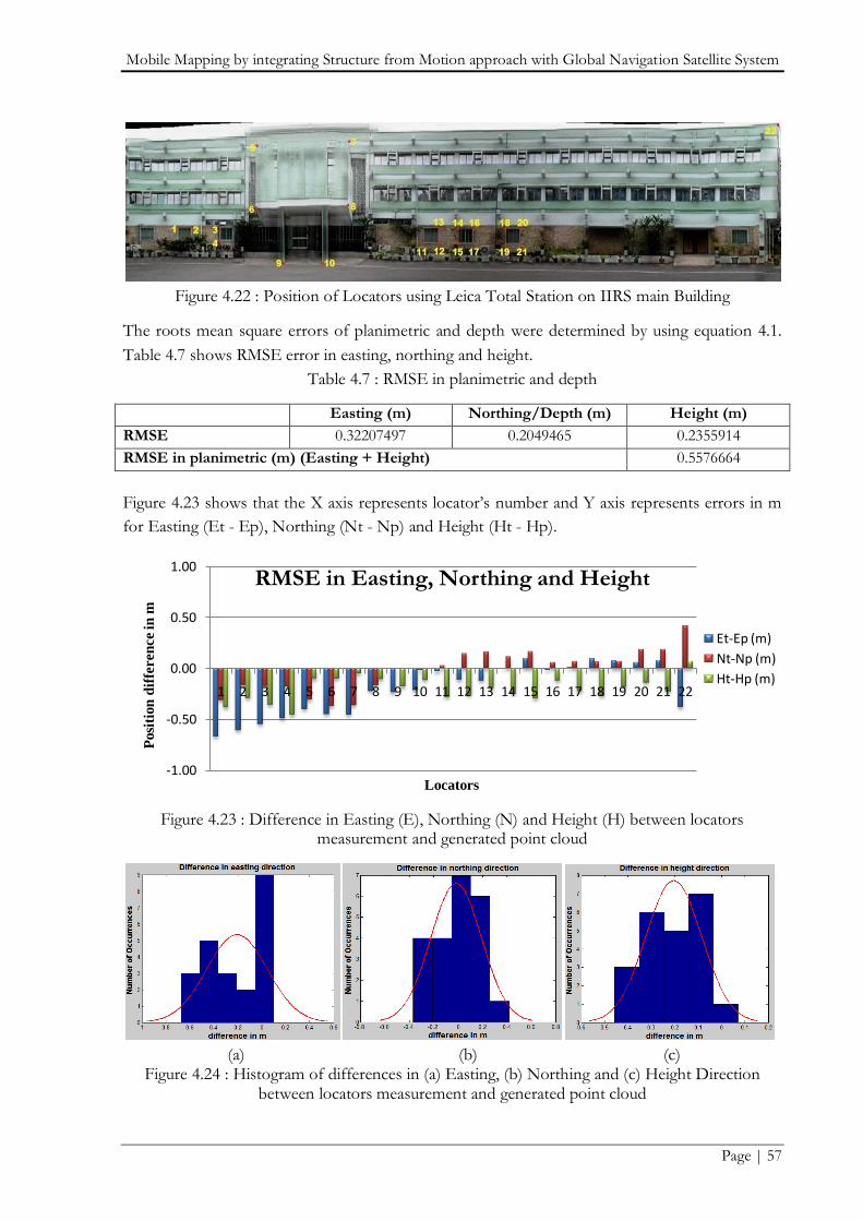
Mobile Mapping by integrating Structure from Motion approach with Global Navigation Satellite System
Page | 57
Figure 4.22 : Position of Locators using Leica Total Station on IIRS main Building
The roots mean square errors of planimetric and depth were determined by using equation 4.1.
Table 4.7 shows RMSE error in easting, northing and height.
Table 4.7 : RMSE in planimetric and depth
Easting (m) Northing/Depth (m) Height (m)
RMSE 0.32207497 0.2049465 0.2355914
RMSE in planimetric (m) (Easting + Height) 0.5576664
Figure 4.23 shows that the X axis represents locator‟s number and Y axis represents errors in m
for Easting (Et - Ep), Northing (Nt - Np) and Height (Ht - Hp).
Figure 4.23 : Difference in Easting (E), Northing (N) and Height (H) between locators measurement and generated point cloud
(a) (b) (c) Figure 4.24 : Histogram of differences in (a) Easting, (b) Northing and (c) Height Direction
between locators measurement and generated point cloud
-1.00
-0.50
0.00
0.50
1.00
1 2 3 4 5 6 7 8 9 10 11 12 13 14 15 16 17 18 19 20 21 22
Posi
tion
dif
feren
ce in
m
Locators
RMSE in Easting, Northing and Height
Et-Ep (m)
Nt-Np (m)
Ht-Hp (m)

Mobile Mapping by integrating Structure from Motion approach with Global Navigation Satellite System
Page | 58
Figure 4.24 shows the histogram of locator differences between total station value and generated
point cloud. As shown in graph, the locators were measured on the both end side of buildings
contain more errors and it will effect on RMSE values. As a result of it, there was 32.2 cm RMSE
in easting and 23.5 cm RMSE in northing because the image orientation done in this software
without ground control points (GCP). As shown in graph, middle locators have very good
accuracy in all 3 direction. If we compare the 1,2,3,4 locators height difference are around 30 cm;
5,6,7,8 locators height difference are around 10 cms; 11 to 21 locators height difference are again
20-30 cms but the lcator no. 22 shows 5 cms height differece. Thus locators which are near to
ground have more height diffrence as comapred to top locators. Errors in the measurement of
total station and DGPS also contribute to the total error budgets of different locators.
Mobile Mapping by integrating Structure from Motion approach with Global Navigation Satellite System
Page | 59
5. CONCLUSION AND RECOMMENDATIONS
5.1. Conclusion
Structure from Motion is an approach to reconstruct the surrounding 3D scene from 2D images
and generate projection matrices of exposure station. In this thesis, a new technique has been
implemented for direct geo-referencing by using SfM approach and space photo intersection with
linearization of collinearity equation. Sometime the epipolar lines do not exactly cross at a fixed
point in different overlapping images and due to which a distorted 3D scene (point cloud) was
created. No ground measurements were used in bundle adjustment, thus there was an error in the
estimation of orientation parameters and it was observed that the shape of the point cloud was
concaved near first and last edges of the scene, there were major error detected in easting and
northing.
5.1.1. Answers of Research questions
1) How reliable are the SIFT and RANSAC algorithms to extract and match proper/correct
corresponding features from sequence of overlapping images?
As per literature study and present work it is observed that SIFT is invariant with rotation, scale
and illumination but it takes more time to extract features from each and every images compared
to other extractors. Performance of an extractor is not only assessed based on feature extraction
but it should also be on the basis of feature matching between sequences of overlapping images.
On the basis of feature matching algorithm ANN and outliers‟ removal algorithm RANSAC, the
percentage of average outliers in consecutive pair of images, non consecutive pair of images and
total outliers were 28.43%, 48.47 % and 40.16% respectively. It seems that there were more than
50 % inliers in sequence of images. Therefore SIFT and RANSAC are reliable for this type of
study.
2) How to integrate GPS measurement with the corresponding feature points to make the whole system geo
referenced and introduce a proper scale in three dimensional point cloud?
In my present study, a new technique was implemented for space photo intersection with least
square optimization and similarity from point correspondences techniques to integrate the
exposure station position with corresponding feature points to make the whole system geo
referenced and with proper scale.
3) How to assess the quality of generated point cloud? What is the accuracy of generated point cloud?
Accuracy assessment is mainly categorized into two parts: Internal Accuracy assessment and
external accuracy assessment. Internal accuracy was assessed by registration error and comparison

Mobile Mapping by integrating Structure from Motion approach with Global Navigation Satellite System
Page | 60
with object model i.e. planarity of planer surface. External accuracy was assessed by ground truth
and comparison with highly dense point cloud. These both assessments are based on statistic
analysis and visualization. For Registration error, it was observed that standard deviation was 4.11
cm around 3.45 cm mean at the time of transforming local coordinate into global coordinate
system using point-based similarity transformation. For Internal Accuracy, It was observed that
distances have standard deviation (6.8 cm, 3.5 cm and 13.6 cm) from the Mean (-1.5 cm, 0 and
1.82 cm) in group 1, 2 and 3 respectively. For External Accuracy, RMSE were 32.21 cm, 20.50
cm and 23.56 cm in easting, northing (depth) and height respectively.
5.2. Recommendations
1) In present work, two different system was used for data acqusition (Camera tripod and
GPS tripod). Instead of these, rig of camera and GPS system can be used which will then
be implemented on moble vehicle. This mobile van includes two cameras with proper
baseline set, two GPS, synchronizer between GPS and camera system, Digital
Measurement Unit.
2) For space photo intersection, Manual selection of matched feature points has been done.
Instead of this, we can make a automated system that will read the feature matching file
and convert that feature point into world coordinate system.
3) In this research work, different software platforms had been used. Instead of this, if we
will make whole system on same software platform, it will reduce computational time and
inefficiency of the system.
4) In my study, pairs of images were used to transfer the local coordinate system into global
coordinate system by applying space photo intersection. The output of bundler is the
rotation parameters of exposure station. We will consider these rotation parameters
values as an initial value in new bundle adjustment with camera exposure station. Then it
will give the final exterior orientation parameter with point cloud in global coordinate
system. And hence higher accuracy can be achieved in the system.
Page | 61
REFERENCES
Al-sadik, B. (2012a, 26th December 2012). Space photo intersection Retrieved 10th Feb 2013, from Available on :: http://www.mathworks.in/matlabcentral/fileexchange/39648-space-photo-intersection
Al-sadik, B. (2012b). Structure from Motion (SfM) Notes of Module 13: 3D Geoinformation from imagery. ITC, university of Twente, Enschede, The Netherlands.
Alhwarin, F., Ristić–Durrant, D., & Gräser, A. (2010). VF-SIFT: very fast SIFT feature matching. Paper presented at the Proceedings of the 32nd DAGM conference on Pattern recognition, Darmstadt, Germany.
Aljoboori, B. S., Albakry, M., & Mansour, F. (2009). Close Range Photogrametry (i. A. language, Trans.) Analytical Photogrammetry (pp. 185-222). Iran.
Arya, S., & Mount, D. M. (2010, 28th Jan 2010). ANN: A Library for Approximate Nearest Neighbor Searching Retrieved 10th Feb 2013, from http://www.cs.umd.edu/~mount/ANN/
Bay, H., Tuytelaars, T., & Van Gool, L. (2006). SURF: Speeded Up Robust Features. Paper presented at the 9th European Conference on Computer Vision, Graz, Autriche.
Brenner, C. (2005). Building reconstruction from images and laser scanning. International Journal of Applied Earth Observation and Geoinformation, 6(3–4), 187-198. doi: 10.1016/j.jag.2004.10.006
Derpanis, K. G. (2010). Overview of the RANSAC Algorithm. Chicago. Dorota, A., Grejner-Brzezinska, Li, R., Haala, N., & Toth, C. (2004). From Mobile Mapping to
Telegeoinformatics: Paradigm Shift in Geospatial Data Acquisition, Processing, and Management. American Society for Photogrammetry and Remote Sensing, 70(2), 197-220.
Ellum, C. (2009). New Strategies for Combining GNSS and Photogrammetric Data. Ph.D., University of Calgary, Calgary, Alberta.
Fischler, M. A., & Bolles, R. C. (1981). Random sample consensus: a paradigm for model fitting with applications to image analysis and automated cartography. Commun. ACM, 24(6), 381-395. doi: 10.1145/358669.358692
Furukawa, Y., & Ponce, J. (2010). Accurate, Dense, and Robust Multi-View Stereopsis. IEEE Trans. on Pattern Analysis and Machine Intelligence, 32(8), 1362-1376.
Gerke, M., Khoshelham, K., & Alsadik, B. (2012). Module 13: 3D GeoInformation from Imagery ITC Lecture Notes: ITC.
Girardeau-Montaut, D. (2012). CloudCompare Software V2 Retrieved 10th Feb 2013, 2013, from Available on : http://www.danielgm.net/cc
Horn, B. K. P. (1987). Closed-form solution of absolute orientation using unit quaternions. Optical Society of America A, 4, 629.
IIRS. (2012, 7th March 2013). History of IIRS and ITC Retrieved 1st January 2013, from www.iirs.gov.in/history%26objectives
ImageMagick. (1999). ImageMagick Mogrify Command-Line Tool Retrieved 10th Feb, 2013, from http://www.imagemagick.org/script/mogrify.php
ISPRS. (2010). Tips for the effective use of close range digital photogrammetry for the Earth sciences. ISPRS - Commission V - Close-Range Sensing: Analysis and Applications Working Group V / 6 - Close range morphological measurement for the earth sciences, 2008-2012.
Juan, L., & Gwun, O. (2009). A Comparison of SIFT, PCA-SIFT and SURF. International Journal of Image Processing (IJIP), 3(4), 143-152.
Ka, Z., Yehua, S., & Chun, Y. (2011). Stereo Image Matching for Vehicle-Borne Mobile Mapping System Based on Digital Parallax Model. International Journal of Vehicular Technology, 2011, 1-11. doi: 10.1155/2011/326865
Page | 62
Khoshelham, K. (2005). Region refinement and parametric reconstruction of building roofs by integration of image and height data. International Archives of Photogrammetry and Remote Sensing, IAPRS : XXXVI, part 3 / W 24, 6.
Khoshelham, K. (2012). Quality of Terrestrial Point Clouds Module 13, M.Sc. Lecture Notes. : ITC. Kiichiro, I., Jun-ichi, T., Yoshiharu, A., & Takumi, H. (2006, 4-6 Oct. 2006). A Mobile Mapping
System for road data capture based on 3D road model. Paper presented at the Computer Aided Control System Design, 2006 IEEE International Conference on Control Applications, 2006 IEEE International Symposium on Intelligent Control, 2006 IEEE.
Kim, J. (2008). Camera parameter estimation for image based modeling Visual recognition and search. Li, W., Li, B., & Li, X. (2008). Camera calibration of the Stereo vision measurement system. Paper
presented at the Advanced Optical and Mechanical Technologies in Telescopes and Instrumentation, China.
Lourakis, M. I. A., & Argyros, A. A. (2009). SBA: A software package for generic sparse bundle adjustment. ACM Trans. Math. Softw., 36(1), 1-30. doi: 10.1145/1486525.1486527
Lowe, D. G. (1999). Object recognition from local scale-invariant features. Paper presented at the Computer Vision, 1999. The Proceedings of the Seventh IEEE International Conference on.
Lowe, D. G. (2001). Local Feature View Clustering for 3D Object Recognition. Paper presented at the IEEE Conference on Computer Vision and
Pattern Recognition, Kauai, Hawaii. Lowe, D. G. (2004). Distinctive Image Features from Scale-Invariant Keypoints. Int. J. Comput.
Vision, 60(2), 91-110. doi: 10.1023/b:visi.0000029664.99615.94 Madani, M. (2001). Importance of Digital Photogrammetry for a complete GIS. Paper presented at the 5th
Global Spatial Data Infrastructure Conference, Cartagena, Columbia. Madsen, K., Nielsen, H. B., & Tingleff, O. (2004). Methods for non-linear least square problems.
Informatics and Mathematical Modelling, Technical University of Denmark. Mikolajczyk, K., Tuytelaars, T., Schmid, C., Zisserman, A., Matas, J., Schaffalitzky, F., . . . Gool,
L. V. (2005). A Comparison of Affine Region Detectors. Int. J. Comput. Vision, 65(1-2), 43-72. doi: 10.1007/s11263-005-3848-x
Naser, E.-S. (2005). An Overview of Mobile Mapping Systems. Cairo, Egypt: Pharaohs to Geoinformatics FIG Working Week 2005 and GSDI-8.
NRC. (1995). GPS Positioning Guide M. a. R. E. The Department of Energy (Ed.) (pp. 123). PhotoModelerScanner. (2013). Photo Modeler Scanner Calibration Tutorials Retrieved 10th Feb,
2013, from Available on : http://www.photomodeler.com/downloads/PM6TutorialStreams/CalibrationPart1.html, http://www.photomodeler.com/downloads/PM6TutorialStreams/CalibrationPart2.html
Piras, M., Cina, A., & Lingua, A. (2008, 5-8 May 2008). Low cost mobile mapping systems: an Italian experience. Paper presented at the Position, Location and Navigation Symposium, 2008 IEEE/ION.
Pollefeys, M., Koch, R., Vergauwen, M., & Van Gool, L. (2000). Automated reconstruction of 3D scenes from sequences of images. Isprs Journal of Photogrammetry and Remote Sensing, 55(4), 251-267. doi: 10.1016/s0924-2716(00)00023-x
Pu, S., & Vosselman, G. (2009). Knowledge based reconstruction of building models from terrestrial laser scanning data. Isprs Journal of Photogrammetry and Remote Sensing, 64(6), 575-584. doi: 10.1016/j.isprsjprs.2009.04.001
Remondino, F., & El-Hakim, S. (2006). Image-based 3D Modelling: A Review. The Photogrammetric Record, 21(115), 269-291. doi: 10.1111/j.1477-9730.2006.00383.x
Sabzevari, R., Bue, A. D., & Murino, V. (2011). Structure from motion and photometric stereo for dense 3D shape recovery. Paper presented at the Proceedings of the 16th international conference on Image analysis and processing: Part I, Ravenna, Italy.

Page | 63
Sande, C. v. d., Soudarissanane, S., & Khoshelham, K. (2010). Assessment of Relative Accuracy of AHN-2 Laser Scanning Data Using Planar Features. Sensors, 10(9), 8198-8214.
Snavely, N. (2010, April 25, 2010). Bundler: Structure from Motion (SfM) for Unordered Image Collections v0.4 Version 0.4. Retrieved 10th Feb, 2013, 2013, from Available on : http://phototour.cs.washington.edu/bundler/#S4
Sunglok, C., Taemin, K., & Wonpil, Y. (2009). Performance Evaluation of RANSAC Family. Paper presented at the British Machine Vision Conference Proceedings, London, UK.
Tian, Y., Gerke, M., Vosselman, G., & Zhu, Q. (2010). Knowledge-based building reconstruction from terrestrial video sequences. Isprs Journal of Photogrammetry and Remote Sensing, 65(4), 395-408. doi: 10.1016/j.isprsjprs.2010.05.001
TPS. (2013). Leica TPS 1200 user manuals. Hexagon: Leica Geosystems Triggs, B., McLauchlan, P. F., Hartley, R. I., & Fitzgibbon, A. W. (2000). Bundle Adjustment - A
Modern Synthesis. Paper presented at the Proceedings of the International Workshop on Vision Algorithms: Theory and Practice.
Vosselman, G. (2012). Point Cloud Mapper : Programme for interactive modelling of buildings in laser scanner point clouds. The Netherlands.
Wackrow, R., Chandler, J. H., & Bryan, P. (2007). Geometric consistency and stability of consumer-grade digital cameras for accurate spatial measurement. Remote Sensing and Photogrammetry Society and Blackwell Publishing Ltd.
Weizheng, Z., Tao, J., & Mingqin, H. (2010, 16-18 Oct. 2010). Digital camera calibration method based on PhotoModeler. Paper presented at the Image and Signal Processing (CISP), 2010 3rd International Congress on.
Wolf, P. R., & Dewitt, B. A. (2004). Space Intersection by Collinearity Elements of Photogrammetry with application in GIS. United States: McGraw Hills Publication.
Xuexian, G., & Sidong, Z. (2009, 19-20 Dec. 2009). A Mobile System Using Lidar and Photogrammetry for Urban Spatial Objects Extraction. Paper presented at the Information Engineering and Computer Science, 2009. ICIECS 2009. International Conference on.
Yan, K., & Sukthankar, R. (2004, 27 June-2 July 2004). PCA-SIFT: a more distinctive representation for local image descriptors. Paper presented at the Computer Vision and Pattern Recognition, 2004. CVPR 2004. Proceedings of the 2004 IEEE Computer Society Conference on.
Yaniv, Z. (2010). Random Sample Consensus (RANSAC) Algorithm, A Generic Implementation. Insight Journal.
Zhan-long, Y., & Bao-long, G. (2008). Image Mosaic Based On SIFT. Paper presented at the Intelligent Information Hiding and Multimedia Signal Processing, Harbin, China.
Zhang, Y., Zhang, Z., Zhang, J., & Wu, J. (2005). 3D Building Modelling with Digital Map, Lidar Data and Video Image Sequences. The Photogrammetric Record, 20(111), 285-302. doi: 10.1111/j.1477-9730.2005.00316.x
Zhu, J. (2006). 3D from Pictures. University of Virginia. Zisserman, A., & Hartley, R. (2001). Relative Orientation Multiple View Geometry in Computer
Vision. University Press, Cambridge.

Page | 64
APPENDICES
Appendix - I: Exposure Station Position Difference
Table 1 : Exposure Station Position Difference in m
No Measured
Distance (m)
Error
(cm)
0 - -
1 2.4510856368 4.89144
2 2.4597543536 4.02456
3 2.4482134752 5.17865
4 2.5526793536 -5.26794
5 2.5131749445 -1.317494
6 2.5340407542 -3.404075
7 2.4781830666 2.181693
8 2.4469267325 5.307327
9 2.4739059794 2.609402
10 2.5659786472 -6.597865
11 2.5147134347 -1.471343
12 2.4564588485 4.354115
13 2.4884343588 1.156564
14 2.5548066837 -5.480668
15 2.5123486711 -1.234867
16 2.4456024060 5.439759
17 2.5613723767 -6.137238
18 2.4555072051 4.449279
19 2.5027162571 -0.271626
20 2.5312636211 -3.126362
21 2.4542267600 4.577324
22 2.5247862215 -2.478622
23 2.4513294314 4.867057
Appendix - II: Features Extraction and Matching
Table 2 : Features Extraction using SIFT
No. Key Points Time No. Key Points Time No. Key Points Time
0 5360 8.09sec 8 3778 0.54sec 16 3370 0.51sec
1 5301 0.65sec 9 3836 0.53sec 17 3536 0.52sec
2 4642 0.60sec 10 3967 0.55sec 18 3899 0.54sec
3 4625 0.59sec 11 3908 0.53sec 19 4229 0.57sec
4 4029 0.62sec 12 3761 0.52sec 20 4985 0.62sec
5 3406 0.52sec 13 3708 0.53sec 21 5320 0.86sec
6 3337 0.56sec 14 3755 0.51sec 22 5881 0.75sec
7 3577 0.53sec 15 3368 0.84sec 23 6761 0.78sec

Page | 65
Table 3 : Features Matching
Pair Feature
Matches
Time
(sec) Pair
Feature
Matches
Time
(sec) Pair
Feature
Matches
Time
(sec) Pair
Feature
Matches
Time
(sec)
0,1 408 1.07 4,8 268 0.47 11,13 391 0.43 15,19 147 0.42
0,2 199 0.51 5,8 360 0.39 12,13 677 0.43 16,19 203 0.40
1,2 440 0.51 6,8 465 0.40 10,14 191 0.50 17,19 352 0.43
0,3 170 0.49 7,8 789 0.41 11,14 243 0.44 18,19 892 0.47
1,3 236 0.49 5,9 329 0.40 12,14 344 0.44 16,20 120 0.42
2,3 551 0.49 6,9 395 0.39 13,14 746 0.42 17,20 193 0.44
0,4 149 0.48 7,9 466 0.42 11,15 165 0.39 18,20 327 0.48
1,4 205 0.48 8,9 816 0.43 12,15 208 0.38 19,20 776 0.50
2,4 319 0.51 6,10 386 0.39 13,15 294 0.37 17,21 131 0.43
3,4 623 0.49 7,10 409 0.44 14,15 543 0.40 18,21 204 0.47
1,5 195 0.41 8,10 526 0.46 12,16 132 0.38 19,21 349 0.51
2,5 287 0.43 9,10 925 0.47 13,16 193 0.37 20,21 643 0.51
3,5 307 0.41 7,11 331 0.44 14,16 297 0.38 18,22 144 0.47
4,5 612 0.41 8,11 439 0.45 15,16 638 0.34 19,22 207 0.48
2,6 210 0.41 9,11 553 0.46 13,17 105 0.40 20,22 270 0.49
3,6 261 0.41 10,11 873 0.46 14,17 144 0.40 21,22 503 0.49
4,6 317 0.41 8,12 328 0.44 15,17 238 0.36 19,23 77 0.49
5,6 718 0.34 9,12 371 0.43 16,17 524 0.37 20,23 114 0.49
3,7 220 0.44 10,12 471 0.45 14,18 129 0.45 21,23 197 0.50
4,7 273 0.43 11,12 791 0.44 15,18 176 0.39 22,23 374 0.50
5,7 438 0.36 9,13 264 0.46 16,18 286 0.39
6,7 805 0.35 10,13 296 0.43 17,18 649 0.41
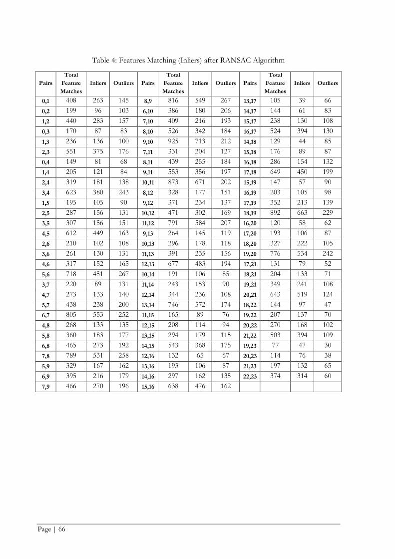
Page | 66
Table 4: Features Matching (Inliers) after RANSAC Algorithm
Pairs
Total
Feature
Matches
Inliers
Outliers Pairs
Total
Feature
Matches
Inliers
Outliers Pairs
Total
Feature
Matches
Inliers
Outliers
0,1 408 263 145 8,9 816 549 267 13,17 105 39 66
0,2 199 96 103 6,10 386 180 206 14,17 144 61 83
1,2 440 283 157 7,10 409 216 193 15,17 238 130 108
0,3 170 87 83 8,10 526 342 184 16,17 524 394 130
1,3 236 136 100 9,10 925 713 212 14,18 129 44 85
2,3 551 375 176 7,11 331 204 127 15,18 176 89 87
0,4 149 81 68 8,11 439 255 184 16,18 286 154 132
1,4 205 121 84 9,11 553 356 197 17,18 649 450 199
2,4 319 181 138 10,11 873 671 202 15,19 147 57 90
3,4 623 380 243 8,12 328 177 151 16,19 203 105 98
1,5 195 105 90 9,12 371 234 137 17,19 352 213 139
2,5 287 156 131 10,12 471 302 169 18,19 892 663 229
3,5 307 156 151 11,12 791 584 207 16,20 120 58 62
4,5 612 449 163 9,13 264 145 119 17,20 193 106 87
2,6 210 102 108 10,13 296 178 118 18,20 327 222 105
3,6 261 130 131 11,13 391 235 156 19,20 776 534 242
4,6 317 152 165 12,13 677 483 194 17,21 131 79 52
5,6 718 451 267 10,14 191 106 85 18,21 204 133 71
3,7 220 89 131 11,14 243 153 90 19,21 349 241 108
4,7 273 133 140 12,14 344 236 108 20,21 643 519 124
5,7 438 238 200 13,14 746 572 174 18,22 144 97 47
6,7 805 553 252 11,15 165 89 76 19,22 207 137 70
4,8 268 133 135 12,15 208 114 94 20,22 270 168 102
5,8 360 183 177 13,15 294 179 115 21,22 503 394 109
6,8 465 273 192 14,15 543 368 175 19,23 77 47 30
7,8 789 531 258 12,16 132 65 67 20,23 114 76 38
5,9 329 167 162 13,16 193 106 87 21,23 197 132 65
6,9 395 216 179 14,16 297 162 135 22,23 374 314 60
7,9 466 270 196 15,16 638 476 162

Page | 67
Appendix - III: Accuracy Assessment between TPS locators and Generated
Point Cloud
Table 6 : Accuracy Assessment between TPS locators and Generated Point Cloud
No Et – Ep
(m)
Nt – Np
(m) Ht – Hp (m)
(Et – Ep) 2
(m)
(Nt – Np) 2
(m)
(Ht – Hp) 2
(m)
1 -0.67199934 -0.31087230 -0.38233319 0.45158311 0.09664159 0.14617867
2 -0.60683875 -0.16389068 -0.28990964 0.36825326 0.02686015 0.08404760
3 -0.54533869 -0.17037858 -0.35891873 0.29739429 0.02902886 0.12882266
4 -0.49239869 -0.17770255 -0.45638483 0.24245647 0.03157820 0.20828711
5 -0.39857325 -0.30668958 -0.10210580 0.15886064 0.09405850 0.01042560
6 -0.44797519 -0.36872650 -0.09929776 0.20068177 0.13595923 0.00986005
7 -0.45409159 -0.36115338 -0.04919007 0.20619917 0.13043176 0.00241966
8 -0.22181061 -0.16916496 -0.10305580 0.04919995 0.02861678 0.01062050
9 -0.23564946 0.00226581 -0.17904321 0.05553067 0.00000513 0.03205647
10 -0.21232079 -0.01559873 -0.11306123 0.04508012 0.00024332 0.01278284
11 -0.03015947 0.02761795 -0.28101330 0.00090959 0.00076275 0.07896847
12 -0.11178481 0.14622185 -0.25873231 0.01249584 0.02138083 0.06694241
13 -0.11861918 0.16306383 -0.19383667 0.01407051 0.02658981 0.03757266
14 -0.00666141 0.11632824 -0.24598821 0.00004437 0.01353226 0.06051020
15 0.10060913 0.16456335 -0.29440874 0.01012220 0.02708110 0.08667651
16 -0.01722751 0.06086486 -0.12017159 0.00029679 0.00370453 0.01444121
17 0.01323619 0.06764195 -0.22357142 0.00017520 0.00457543 0.04998418
18 0.09630770 0.06534524 -0.26760610 0.00927517 0.00427000 0.07161302
19 0.07517866 0.06838920 -0.18186288 0.00565183 0.00467708 0.03307411
20 0.05854123 0.18606028 -0.13980147 0.00342708 0.03461843 0.01954445
21 0.08036130 0.18769375 -0.22668623 0.00645794 0.03522894 0.05138665
22 -0.37940000 0.41740000 0.06970000 0.14394436 0.17422276 0.00485809
Sum of "Power((Et-Ep),2)", "Power((Nt-Np'),2)"
and "Power((Ht-Hp'),2)" 2.28211032 0.92406746 1.2210731
Average :: "Sum(Power((Et-Ep),2))/22", "Sum(Power((Nt-
Np),2))/22"
and "Sum(Power((Ht-Hp'),2))/22" 0.10373229 0.04200307 0.05550332
RMSE 0.32207497 0.2049465 0.23559143
RMSE in planimetric (m) 0.5576664
RMSE in altimetric (m) 0.2049465