Mobility Modeling and Prediction in Bike-Sharing Systems

Zidong Yang†, Ji Hu†, Yuanchao Shu‡∗, Peng Cheng†, Jiming Chen†, Thomas Moscibroda‡

† Zhejiang University, Hangzhou, China ‡ Microsoft Research Asia

ABSTRACT

As an innovative mobility strategy, public bike-sharing has growndramatically worldwide. Though providing convenient, low-costand environmental-friendly transportation, the unique features ofbike-sharing systems give rise to problems to both users andoperators. The primary issue among these problems is the unevendistribution of bicycles caused by the ever-changing usage and(available) supply. This bicycle imbalance issue necessitatesefficient bike re-balancing strategies, which depends highly onbicycle mobility modeling and prediction. In this paper, for thefirst time, we propose a spatio-temporal bicycle mobility modelbased on historical bike-sharing data, and devise a traffic predictionmechanism on a per-station basis with sub-hour granularity. Weextensively evaluated the performance of our design through a one-year dataset from the world’s largest public bike-sharing system(BSS) with more than 2800 stations and over 103 million checkin/out records. Evaluation results show an 85 percentile relativeerror of 0.6 for both check in and check out prediction. We believethis new mobility modeling and prediction approach can advancethe bike re-balancing algorithm design and pave the way for therapid deployment and adoption of bike-sharing systems across theglobe.

Keywords

Sharing economy; Bike sharing; Mobility modeling; Flow predic-tion; Rebalancing

1. INTRODUCTIONShared transportation has grown tremendously in recent years

as a result of the rise of the sharing economy and growingenvironmental, energy and economic concerns. Among the variousforms of shared-use mobility1, public bike-sharing systems (BSS)

∗Yuanchao Shu is the corresponding author of this paper.1Shared-use mobility–the shared use of transportation services–is an innovative transportation solution that enables users to haveshort-term access to transportation modes. It includes traditionalpublic transit, bike-sharing, car-sharing, ride-sharing, ride-sourcingetc.

Permission to make digital or hard copies of all or part of this work for personal orclassroom use is granted without fee provided that copies are not made or distributedfor profit or commercial advantage and that copies bear this notice and the full citationon the first page. Copyrights for components of this work owned by others thanACM must be honored. Abstracting with credit is permitted. To copy otherwise, orrepublish, to post on servers or to redistribute to lists, requires prior specific permissionand/or a fee. Request permissions from permissions@acm.org.

MobiSys’16, June 25-30, 2016, Singapore, Singapore

c© 2016 ACM. ISBN 978-1-4503-4269-8/16/06. . . $15.00

DOI: http://dx.doi.org/10.1145/2906388.2906408

have become increasingly popular with a significant growingpresence over the past decade. Available figures indicate that thereare more than 500 bike-sharing programs running in at least 49countries with one million shared bikes in 2015 [1, 2].

In addition to its advantages of reducing traffic congestion andmitigating pollution, BSS feature unique characteristics comparedwith other forms of shared-use mobility. First, bike-sharing differsfrom classic ride-sharing (e.g., carpooling) and ride-sourcing (e.g.,Uber and Lyft) in that bicycles are typically unattended. Duringvacant hours, bicycles are concentrated at a group of stations whereoperations of checking in or checking out are facilitated througha backbone network, i.e., an IT infrastructure that enables rentmanagement and monitoring. Second, unlike conventional publictransit (e.g., subways and buses) which follows a regular scheduleand pre-determined routes, bike-sharing provides transportationon an on-demand basis with a decentralized structure. Thesetwo distinct features, however, pose characteristic challenges inBSS management and optimization. One common problem, forexample, is that the system typically ends up with an unevendistribution of bikes across the different stations (due to theuncontrolled, uneven demand), often rendering the check in orcheck out service unavailable at some stations where bicycle docksare either fully occupied or empty.

This bicycle imbalance problem makes it necessary for bike-share cities to employ costly bike redistribution, which is typicallyperformed by trucks or trailers driving around the city, movingbikes among stations. To increase service availability and minimizeredistribution cost, studies have been conducted to improve thesebike redistribution strategies based on bicycle mobility models andpredictions. Yet, in spite of the researches on bike usage patternsand global rental volume forecasts (e.g., [3–7]), developing a fine-grained and localized prediction model for the number of bikesthat should be optimally redistributed has proven to be elusive,and has remained a largely unstudied problem. The main technicalchallenge is that bike traffic is not only highly dynamic and inter-correlated in both the temporal and spatial domains, but also furtherinfluenced by complex issues such as timing and meteorology.

In this paper, we establish a spatio-temporal mobility modelof bikes, and present a novel fine-grained traffic (i.e., check inand check out) prediction mechanism on a per-station basis byleveraging historical bike-sharing data as well as meteorologicaldata. Our work differs fundamentally from previous approaches inthat we model BSS as a dynamic network and predict the trafficby jointly considering the spatio-temporal correlations betweenstations and additional time factors and meteorology. To this end,we first decouple the bicycle transitions between stations fromcheck out actions based on the counterbalance of bicycles andthe mutual independence of user behaviors. Based on historical

165

data, we then use a probabilistic model to describe the spatio-temporal movements of bikes within the network, and estimate thenumber and time of check in at different stations. Combined witha random-forest-based check out prediction algorithm, we are ableto estimate the number of docked bicycles at each station at anygiven time period in the future, which lays a foundation for efficientredistribution strategy design.

This paper makes the following three main contributions:

• We identify the mobility modeling problem and establish aspatio-temporal dynamic network model for BSS by takinginto account the interactions among all stations;

• To our knowledge, we conduct the first work to devise atraffic prediction mechanism on a per-station basis with sub-hour granularity by using the mobility model and historicaldata;

• We evaluate the performance of mobility modeling andprediction through a one-year dataset from the city ofHangzhou, the world’s largest public BSS with more than2800 stations and over 103 million check in/out records [8,9]. Compared with two benchmark methods, the proposedapproach provides the best performance with an 85 percentilerelative error of 0.6 for both check in and check outprediction.

The remainder of this paper is organized as follows. We firstprovide an overview of our design in Section 2. We then presentthe mobility model in Section 3, followed by detailed illustration ofbicycle check out prediction in Section 4. Section 5 describes ourdatasets, and Section 6 presents an in-depth evaluation of mobilitymodeling and prediction. Several insights and related work arediscussed in Section 7 and Section 8. We conclude the paperin Section 9.

2. DESIGN OVERVIEWThis section provides a design overview, including problem

formulation in Section 2.1 and design methodology in Section 2.2.

2.1 Problem FormulationTwo types of entities constitute a BSS system (see Figure 1):

Active objects (users) and Reactive objects (bikes), respectively.Users shift bikes from check in to check out operations, changingthe status (i.e., the number of docked bicycles) of stations locatedat different places. Conversely, the spatial diversity of stations andbike availabilities also influence user behaviors. In this paper, wecall a sequence of operations - bicycle check out, movement andcheck in - a shift instance (SI). As can be seen from Figure 1, Active

objects and Reactive objects are coupled in both the temporal andspatial domain. However, it is worth noting that user activitiesin Active objects are mutually independent, though subject to thechange of time factors and meteorology.

The objective of this paper is two-fold. First, we aim tomodel the mobility patterns of bikes in BSS. The mobilitymodel characterizes the spatio-temporal transition of bikes amongstations. Second, based on the mobility model, we aim to predictthe number of docked bicycles at each station at a given timein the future. Due to the correlation between Active objects andReactive objects as well as among stations, our design methodologyproceeds from a decoupling operation, which disentangles thesevarious correlations.

User

User

User

User

User

User Station

Station

Station

Station

Station

Station

User

User

User

Check out, Riding, Check in

Station distribution, Bike availability

Reactive objectActive object

Time factors, meteorology

Figure 1: Components of a bike-sharing system.

2.2 Design MethodologyDespite the random bicycle check out time and location in each

SI, bicycles are bound to be checked in at some station. Based onthis simple observation, we decouple the system in Figure 1 intotwo parts (i.e., the left blue part and the right red part with dashedlines) by modeling the mobility of undocked bicycles and checkout behaviors separately. Specifically, based on historical checkout data, we first use a probabilistic model to describe the spatio-temporal movements of the undocked bikes, and then estimate thenumber and time of check in at different stations (see Section 3).We then apply the random forest theory to model and predictthe users’ check out behaviors with a joint consideration of timefactors, meteorology and real-time bike availability (see Section 4).Both estimation and prediction results are updated in an onlinemanner, and therefore can be integrated into any existing real-worldBSS and used to infer and predict the number of docked bicycles ateach station in real time.

3. BICYCLE MOBILITY MODELINGIn this section, we develop a mobility model to capture the

spatio-temporal transition of bikes. The model is establishedbased on the uniqueness of bike flows between different pairs ofstations at different times. For example, bicycles flow into stationsin working areas in the morning on weekdays and flow out inthe afternoon. Even for a random bicycle check out at a givenstation and a given time, the probabilities of the correspondingcheck in at different stations vary. Therefore, we propose astatistical model which uses historical check in/out data to describethe spatio-temporal shifts of bikes between pairs of stations, andestimate bicycle check in based on the online check out records.Compared with state-of-art approaches [10, 11] that treat eachstation independently, our model has the following two advantages:

• Fine-grained Modeling. A fine-grained mobility modelwith time-varying parameters is built based on the analysisof historical bicycle flows between stations. Check inestimations at each station can be obtained using this model.

• Online Updating. The estimation results are continuouslyupdated based on recent check in and check out data,adapting to evolving user behaviors and network settings.

3.1 Theoretical Mobility ModelWe first present a theoretical mobility model which estimates

the check in numbers based on the analysis of historical SI data.Notations are defined in Table 1.

Without loss of generality, we consider the check in estimationof some station i. Given previous check out records (i.e., bikeschecked out before tnow), we aim to quantify bikes that will bechecked in at station i during a target period [t, t+∆] in the future.

166

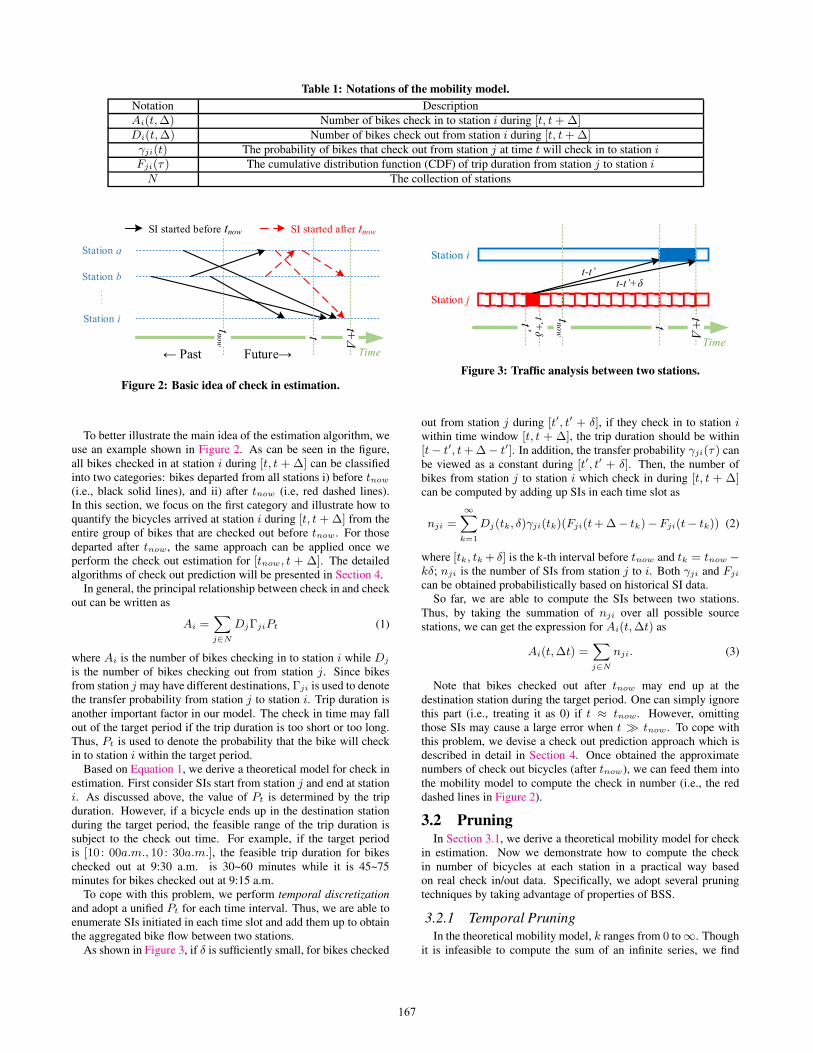
Table 1: Notations of the mobility model.

Notation Description

Ai(t,∆) Number of bikes check in to station i during [t, t+∆]Di(t,∆) Number of bikes check out from station i during [t, t+∆]γji(t) The probability of bikes that check out from station j at time t will check in to station iFji(τ ) The cumulative distribution function (CDF) of trip duration from station j to station iN The collection of stations

Station a

Station b

Station i

tnow

Future→← Past

t

t+Δ

SI started before tnow SI started after tnow

Time

Figure 2: Basic idea of check in estimation.

To better illustrate the main idea of the estimation algorithm, weuse an example shown in Figure 2. As can be seen in the figure,all bikes checked in at station i during [t, t + ∆] can be classifiedinto two categories: bikes departed from all stations i) before tnow

(i.e., black solid lines), and ii) after tnow (i.e, red dashed lines).In this section, we focus on the first category and illustrate how toquantify the bicycles arrived at station i during [t, t +∆] from theentire group of bikes that are checked out before tnow. For thosedeparted after tnow, the same approach can be applied once weperform the check out estimation for [tnow, t + ∆]. The detailedalgorithms of check out prediction will be presented in Section 4.

In general, the principal relationship between check in and checkout can be written as

Ai =∑

j∈N

DjΓjiPt (1)

where Ai is the number of bikes checking in to station i while Dj

is the number of bikes checking out from station j. Since bikesfrom station j may have different destinations, Γji is used to denotethe transfer probability from station j to station i. Trip duration isanother important factor in our model. The check in time may fallout of the target period if the trip duration is too short or too long.Thus, Pt is used to denote the probability that the bike will checkin to station i within the target period.

Based on Equation 1, we derive a theoretical model for check inestimation. First consider SIs start from station j and end at stationi. As discussed above, the value of Pt is determined by the tripduration. However, if a bicycle ends up in the destination stationduring the target period, the feasible range of the trip duration issubject to the check out time. For example, if the target periodis [10 : 00a.m., 10: 30a.m.], the feasible trip duration for bikeschecked out at 9:30 a.m. is 30~60 minutes while it is 45~75minutes for bikes checked out at 9:15 a.m.

To cope with this problem, we perform temporal discretization

and adopt a unified Pt for each time interval. Thus, we are able toenumerate SIs initiated in each time slot and add them up to obtainthe aggregated bike flow between two stations.

As shown in Figure 3, if δ is sufficiently small, for bikes checked

tnow

t

t+Δ

Time

Station j

Station i

t-t’t-t’+δ

t’ t’+

δ

Figure 3: Traffic analysis between two stations.

out from station j during [t′, t′ + δ], if they check in to station iwithin time window [t, t + ∆], the trip duration should be within[t− t′, t+∆− t′]. In addition, the transfer probability γji(τ ) canbe viewed as a constant during [t′, t′ + δ]. Then, the number ofbikes from station j to station i which check in during [t, t + ∆]can be computed by adding up SIs in each time slot as

nji =∞∑

k=1

Dj(tk, δ)γji(tk)(Fji(t+∆− tk)−Fji(t− tk)) (2)

where [tk, tk + δ] is the k-th interval before tnow and tk = tnow −kδ; nji is the number of SIs from station j to i. Both γji and Fji

can be obtained probabilistically based on historical SI data.So far, we are able to compute the SIs between two stations.

Thus, by taking the summation of nji over all possible sourcestations, we can get the expression for Ai(t,∆t) as

Ai(t,∆t) =∑

j∈N

nji. (3)

Note that bikes checked out after tnow may end up at thedestination station during the target period. One can simply ignorethis part (i.e., treating it as 0) if t ≈ tnow. However, omittingthose SIs may cause a large error when t ≫ tnow. To cope withthis problem, we devise a check out prediction approach which isdescribed in detail in Section 4. Once obtained the approximatenumbers of check out bicycles (after tnow), we can feed them intothe mobility model to compute the check in number (i.e., the reddashed lines in Figure 2).

3.2 PruningIn Section 3.1, we derive a theoretical mobility model for check

in estimation. Now we demonstrate how to compute the checkin number of bicycles at each station in a practical way basedon real check in/out data. Specifically, we adopt several pruningtechniques by taking advantage of properties of BSS.

3.2.1 Temporal Pruning

In the theoretical mobility model, k ranges from 0 to ∞. Thoughit is infeasible to compute the sum of an infinite series, we find

167

people usually use public bikes for the last miles of a commute fora short time. In other words, it is reasonable to set a cut off valueon k to perform a temporal pruning.

Take the bike-sharing system in Hangzhou as an example. Thedistribution function of trip durations is depicted in Figure 42. Itdemonstrates that 99.6% SIs are completed within 3 hours. Thus,instead of summing k from 0 to ∞, we can safely set a limit on kto 3 hours.

Time (minutes)

0 30 60 90 120 150 180

CD

F

0

0.2

0.4

0.6

0.8

1Trip duration

Figure 4: CDF of trip duration.

3.2.2 Spatial Pruning

In the theoretical model, SIs between any two stations are takeninto consideration. However, we find it is not essential since thetraffic between two far away stations is usually small and can beignored. In other words, instead of taking all possible sourcestations into consideration, we use a subset of them to computethe potential check in bikes.

Let Mi(n) denote the top-n source stations of station i in termsof the number of check in bicycles, and nji denote the numberof bikes from station j to station i. We further define the top-ncumulative contribution rate λi(n) as follows:

λi(n) =

∑

j∈Mi(n) nji∑

j∈N nji

. (4)

The average, minimal and maximal value of λi(n) over allstations is depicted in Figure 5, which demonstrates that themajority of check in bikes of a specific station can be attributed toa small group of source stations. For example, the top 200 stationscontribute more than 96.6% of bikes on average. Thus, we canperform a spatial pruning by limiting the number of source stationsto a small value. Specially, we rank the numbers of SIs betweeneach pair of source station and target station3, and select the top200 ones (at most) in check in estimation.

3.2.3 γji(t) Discretization and Calculation

It is also worth investigating how to efficiently update theparameter γji(t). By examining the SI data between stations, wefind that γji is highly volatile within a day whereas it remainsrelatively stable across days. Also, due to the sporadic check outof bicycles, we discretize γji(t) into a piece-wise function, andcompute its value within each time slot (e.g., one hour) basedon historical bicycle check in/out data. In the proposed mobilitymodel, we set the length of each time slot to one hour to get atradeoff between the computational overhead and accuracy.

By utilizing the above pruning techniques, it is computationallyfeasible to build a bicycle mobility model and perform check in

2The detailed dataset description is presented in Section 5.3A time slot is set to 1 hour in our paper.

0 200 400 600 800 10000

0.2

0.4

0.6

0.8

1

1.2

n

λ

maxi λ(n)λ(n)mini λ(n)

Figure 5: Cumulative contribution rate.

estimations. In short, our model consists of two phases, namelya training phase and an estimation phase. In the training phase,model parameters (e.g, γji and Fji) are calculated from historicaldata while estimations are conducted by leveraging the model andonline check out records during the estimation phase. The trainingand estimation algorithm for one station is presented in Algorithm 1and Algorithm 2, respectively.

Input : Training dataset S, Number of source stationconsidered m

Output: Mobility model of station i1 modeli = NULL;2 for each time slot t do

3 sources = TopSource (m);4 for each station j ∈ sources do

5 Compute γji for time slot t;6 Estimate trip duration CDF Fji from j to i;7 Add γji, Fji to modeli;

8 end

9 end

10 return modeliAlgorithm 1: Mobility modeling training.

In the training phase, for each time slot, Algorithm 1 computesγji and Fji between top-m source stations and the target station.Thus, the computation complexity for each station is O(nm) wheren is the number of time slots and m is the number of consideredsource stations. In the estimation phase, for each time interval,Algorithm 2 estimates the traffic between each pair of sourcestation and target station. Thus, the corresponding computationcomplexity is O(pm) where p is the number of time intervals. Bothalgorithms can run in parallel, therefore being applied to all stationssimultaneously in a large bike-sharing system. Due to the changesin BBS (e.g., new station deployment) and external conditions (e.g.,road construction), we train the mobility model every one week byusing all SI data from the past one year.

4. BICYCLE CHECK OUT PREDICTIONSection 3 presents a mobility model with check in analysis based

on SIs started before tnow. In this part, we introduce how to predictthe number of bicycle check out after tnow, thus completing themobility model to obtain the total number of check in bicyclesbetween [t, t+∆].

Different from bicycle check in results which are correlated withstations, users’ check out actions are mutually independent butsubject to external factors such as time factors and meteorology.Therefore, we apply random forest theory [12] to model and fore-cast the check out behaviors based on historical SIs, correspondingtime and meteorology data.

168

Input : Mobility model modeli, Estimation time period[t, t+∆], kmax, δ

Output: Estimation result n1 n = 0, k = 1;

2 p = ∆δ

;3 while k < kmax do

4 sources = GetSource (modeli,t+∆− kδ);5 for each station j in sources do

6 Compute Dj(t+∆− kδ, δ);7 Get γji from modeli;8 Get Fji(kδ) from modeli;9 if k ≥ p then

10 // bikes depart before t11 Get Fji(kδ −∆) from modeli;12 n =

n+Dj(t+∆−kδ, δ)γji(Fji(kδ)−Fji(kδ−∆);

13 else

14 // bikes depart after tn = n+Dj(t+∆− kδ, δ)γjiFji(kδ);

15 end

16 end

17 k = k + 1

18 end

19 return nAlgorithm 2: Check in estimation.

4.1 Feature ExtractionWe first extract features from raw data and create feature vectors

with fixed-size time window to build the random forest model. Thefeatures that affect the check out behaviors in a significant way canbe categorized into two types: offline features and online features.

4.1.1 Offline Features

Time factors: Although characteristics of check out actionsdiffer among stations, they are all closely related to time factorsand show unique temporal patterns. We select the most significantfour time factors: day of week, time of day, weekday and holiday.

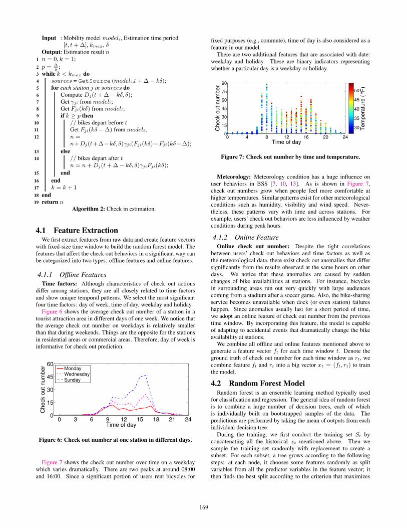
Figure 6 shows the average check out number of a station in atourist attraction area in different days of one week. We notice thatthe average check out number on weekdays is relatively smallerthan that during weekends. Things are the opposite for the stationsin residential areas or commercial areas. Therefore, day of week isinformative for check out prediction.

0 3 6 9 12 15 18 21 240

15

30

45

60

Time of day

Check o

ut num

ber

MondayWednesdaySunday

Figure 6: Check out number at one station in different days.

Figure 7 shows the check out number over time on a weekdaywhich varies dramatically. There are two peaks at around 08:00and 16:00. Since a significant portion of users rent bicycles for

fixed purposes (e.g., commute), time of day is also considered as afeature in our model.

There are two additional features that are associated with date:weekday and holiday. These are binary indicators representingwhether a particular day is a weekday or holiday.

0 4 8 12 16 20 240

15

30

45

60

75

90

Time of day

Ch

eck o

ut

nu

mb

er

Te

mp

era

ture

( °F

)

30

35

40

45

50

Figure 7: Check out number by time and temperature.

Meteorology: Meteorology condition has a huge influence onuser behaviors in BSS [7, 10, 13]. As is shown in Figure 7,check out numbers grow when people feel more comfortable athigher temperatures. Similar patterns exist for other meteorologicalconditions such as humidity, visibility and wind speed. Never-theless, these patterns vary with time and across stations. Forexample, users’ check out behaviors are less influenced by weatherconditions during peak hours.

4.1.2 Online Feature

Online check out number: Despite the tight correlationsbetween users’ check out behaviors and time factors as well asthe meteorological data, there exist check out anomalies that differsignificantly from the results observed at the same hours on otherdays. We notice that these anomalies are caused by suddenchanges of bike availabilities at stations. For instance, bicyclesin surrounding areas run out very quickly with large audiencescoming from a stadium after a soccer game. Also, the bike-sharingservice becomes unavailable when dock (or even station) failureshappen. Since anomalies usually last for a short period of time,we adopt an online feature of check out number from the previoustime window. By incorporating this feature, the model is capableof adapting to accidental events that dramatically change the bikeavailability at stations.

We combine all offline and online features mentioned above togenerate a feature vector ft for each time window t. Denote theground truth of check out number for each time window as rt, wecombine feature ft and rt into a big vector xt = (ft, rt) to trainthe model.

4.2 Random Forest ModelRandom forest is an ensemble learning method typically used

for classification and regression. The general idea of random forestis to combine a large number of decision trees, each of whichis individually built on bootstrapped samples of the data. Thepredictions are performed by taking the mean of outputs from eachindividual decision tree.

During the training, we first conduct the training set St byconcatenating all the historical xt mentioned above. Then wesample the training set randomly with replacement to create asubset. For each subset, a tree grows according to the followingsteps: at each node, it chooses some features randomly as splitvariables from all the predictor variables in the feature vector; itthen finds the best split according to the criterion that maximizes

169

the homogeneity of the two resulting groups. In our design, weuse a mean square error function to measure the quality of a split;at the next node, the procedure is repeated and the training set ispartitioned into smaller groups.

Online check out #

<= 14.5

Time <= 8.5 Time <= 20.4

TemperatureF

<= 37.7

Sample = 36

Value = 25.5

Sample = 14

Value = 7.8

Humidity

<= 79

Sample = 104

Value = 28.8

Sample = 17

Value = 14.3

Sample = 20

Value = 10.9

Sample = 15

Value = 3.8

Yes No

Yes No Yes No

NoYesYes No

Figure 8: A decision tree in random forest.

Figure 8 shows an example decision tree with four layers. Topredict the check out number of time t+1, the input feature vectorft+1 must contain the following fields: day of week, hour of day,holiday, weekday, the meteorology forecast value at time t+1 andonline check out number. When ft+1 is entered into the tree, itneeds to make a decision at each node based on the split variableand makes its way down till it reaches a leaf node. For example, inthis figure, if the online check out number is smaller than or equalto 14.5, the next step is to decide whether time is larger than 8.5. Ifnot, it will reach a leaf node where sample = 36 and value = 25.5. Itmeans that there are 36 samples in the historical SIs that also meetthe above conditions and the value 25.5 is the average check outnumber of those 36 samples. Let yn be the prediction of the nth

single decision tree. Then p = 1Ntree

∑Ntree

n=1 yn is the final checkout prediction.

For online check out prediction, the time window is set to 30minutes. At time window t, we predict check out number for Ksteps to feed the mobility model, i.e., computing {pstep}

Kstep=1.

Under this situation, the input sequence depends on the groundtruth of check out numbers from time window t to time windowt + K − 1, which is unknown by now. Hence we consider thecheck out prediction at time t as the ground truth and use it asan input feature for prediction in the next step. The detailedalgorithm is shown in Algorithm 3. When it comes to the next timewindow, the preceding prediction sequence is discarded and weupdate prediction with new observations. Similar to the mobilitymodel, we update the random forest model every one week.

Input : Training dataset St, prediction horizon length KOutput: Check out prediction {pstep}

Kstep=1

1 Initialize step = 1;2 for each station j do

3 Use St to train the random forest model;4 Compute feature importance for station j;5 while step < K do

6 predict the check out number pstep given observationfstep ;

7 combine the perdition pstep and other offline featuresto fstep+1;

8 step = step + 1;

9 end

10 end

Algorithm 3: Check out prediction for K steps.

Compared with other algorithms, the proposed random forest-based model has the following advantages:

• It can deal with both categorical and numerical variableswithout normalization. In our original data, some mete-orology features such as temperature and wind speed arenumerical variables while holiday and weekday are binaryvariables. We can just take these features as input withoutadditional conversion.

• It provides importance of features based on the trainingdataset, which sheds light on the check out patterns. Forexample, meteorology features may have higher importanceon stations near tourist attractions.

• It can deal with huge volumes of data and can be easilyparallelized, and thus is very suitable for check out behaviormodeling based on millions of SIs.

Denote the length of the training set St as N , the length ofthe test dataset as T . The complexity of feature extraction isO(N+KT ). With regard to the random forest building with Ntree

number of trees, the complexity is O(Ntree ∗ Nlog(N)). Hence,the total computation complexity is O(Nlog(N)).

4.3 Putting It All TogetherIn Section 3 and Section 4, we are able to predict SIs from

two aspects: mobility modeling with check in estimation, andcheck out prediction. The combination of two parts presents acomplete picture of the bike-sharing system. Specifically, for checkout prediction in Section 4, we utilize a random forest modelto capture the relationship between check out behaviors and keyfactors, including time/date, meteorology, and recent check outstatus. Then, given these features, we are able to predict checkout instances in a future period.

In Section 3, we leverage the spatio-temporal relationshipsbetween pairs of stations and derive a probabilistic model todescribe the bike mobility. By feeding both check out records inthe past (i.e., the black lines in Figure 2) and the predicted resultsin the future (i.e., the red dashed lines in Figure 2) into the mobilitymodel, we are able to estimate the check in numbers at each stationat any given period in the future. In addition, the number of dockedbicycles at each station can be inferred by integrating the check inand check out prediction results, which is of great value to bothcustomers and system operators.

5. DATASET DESCRIPTIONBefore presenting performance evaluations, in this section, we

first describe the two datasets used in this paper: the BSS Dataset

and the Meteorology Dataset. The BSS dataset is provided byHangzhou Public Bicycle Transport Service Development Co.,Ltd., and the meteorology dataset was collected from an onlineweather service provider Weather Underground4 .

5.1 BSS DatasetThe Chinese city of Hangzhou has the world’s largest public BSS

with more than 3300 stations and over 84,000 shared bicycles [8,9]. The system adopts smart-card technology and automated checkin and check out. Each check in and check out instance will berecorded in the back-end database with corresponding user ID,bicycle ID, time and etc.

The BSS dataset we use includes all bicycle sharing records in2013. In summary, it contains 43705 bikes and 2806 stations,

4http://www.wunderground.com

170

Table 2: Primary fields in the BSS dataset.

user_id rent_netid tran_date tran_time

6114381 4051 20130101 000152

return_netid return_date return_time bike_id

4015 20130101 001547 913672

among which 103,661,080 trips are recorded. Each bike-sharingrecord has 47 fields, of which the primary fields are shownin Table 2. In 2013, the operational hour for check out serviceranges from 6:00am to 9:00pm while the check in service isavailable until 11:00pm. In order to provide a better overview,we report statistical results of the dataset in terms of stationdistribution, station capacity and usage amount.

Station distribution: Bike stations in Hangzhou are locatedwithin the urban area spanning over 600 square kilometers; theaverage distance to the closest neighboring station being 300meters [8]. The probability distribution function (PDF) of thenumber of stations within a certain range of one station is depictedin Figure 9. As we can see, half the stations have more than 3neighbors within the range of 300 meters, and they typically have20 neighbors within the range of 800 meters.

Figure 9: PDF of the number of stations within a certain range

of one station.

Station capacity: Station capacity is measured as the numberof stocks. As is shown in Figure 10, there are basically two typesof stations in Hangzhou: normal stations with 21 docks and largestation with around 33 docks.

Figure 10: Distribution of station capacity.

Usage amount: Figure 11 presents the distribution of monthlyusage amount (i.e., check in numbers) across all 2806 stations.We find that there are more than 100 busy stations with extremelyhigh usage amount up to 30000 (check in/month). However, themedian value of the usage amount is around 2000. The skeweddistribution in Figure 11 indicates a high diversity of usage amountacross different stations. We observe a similar pattern for check outnumbers.

2

10

20

30

1 2 3 4 5 6 7 8 9 10 11 12Month

Check o

ut num

ber

/10^3

Figure 11: Distribution of monthly usage amount.

Table 3: Fields in the meteorology dataset.

Time (CST) Temp (◦F) Dew Point (◦F)

12:30 PM 100.4 69.8

Pressure (hPa) Humidity (%) Visibility (MPH)

29.65 37 6.2

Wind Dir Wind Speed (MPH) Conditions

WSW 8.9 Partly Cloudy

5.2 Meteorology DatasetThe meteorology dataset contains weather conditions of Hangzhou

with totally 48 × 365 = 17, 520 records. Meteorologicalobservations were updated every half hour and the data format ofeach record is shown in Table 3.

6. EVALUATIONWe conduct extensive data-driven simulations to evaluate the

performance of our design. In the following, we first present theperformance of check out prediction, and then show the checkin estimation results based on the mobility model and check outprediction. Both case studies and overall performance are shown toprovide a more comprehensive analysis.

6.1 Baseline ApproachesWe first introduce three prediction techniques that comprise the

baselines of our model.

• Historical Average (HA) uses the average of historicalobservations for the same time and location to forecast thefuture data [11]. Specially, when conducting prediction fora specific time period, we first find out historical days withsame day/time values, and then average the check in/outresults from these periods.

• Auto-Regressive and Moving Average (ARMA) is widelyused for time series prediction and was adopted for BBScheck in estimation [5]. It leverages check in/out informationof the most recent p time windows for future prediction.Parameters are determined using historical data and the leastsquares method.

• HP-MSI and P-TD are the most recent studies of trafficprediction in bike-sharing system [7] where HP-MSI andP-TD are designed for check out and check in prediction,respectively. Since these two methods are applied to predict

171

traffic amount between clusters of stations, they cannot bedirectly compared with our station-basis design. As anapproximation, we treat each station as an individual clusterin our evaluation.

For performance metrics, we adopt CDFs of both absolute andrelative prediction error. In addition, we also use Root MeanSquared Logarithmic Error (RMLSE) [7] for evaluation. RMLSEis computed as

RMSLE =

√

√

√

√

1

n

n∑

i=1

(log(y + 1) − log(y + 1))2 (5)

where y and y are prediction and ground truth respectively while nis number of predictions.

6.2 Check Out PredictionIn this part, we evaluate the check out prediction model presented

in Section 4, which serves as a component for check in estimation.

6.2.1 Case Studies

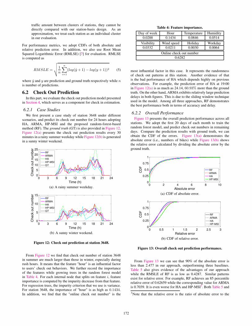
We first present a case study of station 3648 under differentscenarios, and predict its check out number for 24 hours adoptingHA, ARMA, HP-MSI and the proposed random-forest-basedmethod (RF). The ground truth (GT) is also provided in Figure 12.Figure 12(a) presents the check out prediction results every 30minutes in a rainy summer weekday while Figure 12(b) is generatedin a sunny winter weekend.

Time (h)

0 3 6 9 12 15 18 21 24

Check o

ut num

ber

0

5

10

15

20

25RF

ARMA

HA

HP-MSI

GT

(a) A rainy summer weekday.

Time (h)

0 3 6 9 12 15 18 21 24

Check o

ut num

ber

0

5

10

15RF

ARMA

HA

HP-MSI

GT

(b) A sunny winter weekend.

Figure 12: Check out prediction at station 3648.

From Figure 12 we find that check out number of station 3648in summer are much larger than those in winter, especially duringrush hours. It means that the feature "hour" is an influential factorto users’ check out behaviors. We further record the importanceof the features while growing trees in the random forest modelin Table 4. For each internal node that splits on feature i, featureimportance is computed by the impurity decrease from that feature.For regression trees, the impurity criterion that we use is variance.For station 3648, the importance of "hour" is as high as 0.1434.In addition, we find that the "online check out number" is the

Table 4: Feature importance.

Day of week Hour Temperature Humidity

0.0288 0.1434 0.0846 0.0514

Visibility Wind speed Holiday Workday

0.0332 0.0211 0.0030 0.0064

Online check out number

0.6282

most influential factor in this case. It represents the randomnessof check out patterns at this station. Another evidence of thatis the bad performance of HA which depends highly on previousobservations. For example, the prediction error of HA at 19:00in Figure 12(a) is as much as 24.14, 60.93% more than the groundtruth. On the other hand, ARMA exhibits relatively large predictiondelays in both figures. This is due to the sliding window techniqueused in the model. Among all three approaches, RF demonstratesthe best performance both in terms of accuracy and delay.

6.2.2 Overall Performance

Figure 13 presents the overall prediction performance across allstations. We adopt the first 20 days of each month to train therandom forest model, and predict check out numbers in remainingdays. Compare the prediction results with ground truth, we canobtain the CDF of the errors. Figure 13(a) demonstrates theabsolute error (i.e., numbers of bikes) while Figure 13(b) showsthe relative error calculated by dividing the absolute error by theground truth.

Absolute error

0 2 4 6 8 10

CD

F

0

0.25

0.5

0.75

1

RF

ARMA

HA

HP-MSI

(a) CDF of absolute error.

Relative error

0 0.5 1 1.5 2 2.5 3

CD

F

0

0.25

0.5

0.75

1

RF

ARMA

HA

HP-MSI

(b) CDF of relative error.

Figure 13: Overall check out prediction performance.

From Figure 13 we can see that 90% of the absolute error isless than 2.477 in our approach, outperforming three baselines.Table 5 also gives evidence of the advantages of our approachwhile the RMSLE of RF is as low as 0.4287. Similar patternsexist for relative error. For example, RF achieves an 85 percentilerelative error of 0.62659 while the corresponding value for ARMAis 0.7039. It is even worse for HA and HP-MSI5. Both Table 5 and

5Note that the relative error is the ratio of absolute error to the

172

Table 5: RMSLE of check out prediction.

RF ARMA HA HP-MSI

0.4287 0.4855 0.4600 0.4662

Figure 13 prove the effectiveness of the proposed random-forest-based model which takes both time factors, meteorology and real-time check out behaviors into consideration.

6.3 Check In EstimationIn this section, we evaluate the effectiveness of the proposed

mobility model (MM) by demonstrating the results of check inestimations.

6.3.1 Case Studies

Similar to the previous section, we first present two case studiesof a rainy summer weekend and a sunny winter weekday to provideintuitive feelings of performances of different approaches.

Time (h)

0 3 6 9 12 15 18 21 24

Ch

eck in

nu

mb

er

0

5

10

15

20

25

30MM

HA

ARMA

P-TD

GT

(a) A rainy summer weekend.

Time (h)

0 3 6 9 12 15 18 21 24

Ch

eck in

nu

mb

er

0

5

10

15

20MM

HA

ARMA

P-TD

GT

(b) A sunny winter weekday.

Figure 14: Check in prediction at station 3648.

As can be seen from Figure 14, MM is close to the ground truth.However, HA brings larger estimation error because it lacks onlineinformation. Similar to Figure 12, AR suffers from an estimationdelay. As for P-TD, it tends to underestimate the result.

6.3.2 Overall Performance

We also evaluate the overall performance of check in estimationof all three approaches. Specifically, each approach is requiredto estimate check in number in the following 30 minutes (i.e.,∆ = 30). Similar to the random-forest-based model, we train eachmobility model using SIs from the first 20 days of each month, anduse the remaining days for testing. The CDF of absolute error andrelative error is depicted in Figure 15, while RMSLE results arepresented in Table 6.

As one can see from Figure 15(a), for absolute error, allapproaches are quite close when absolute error is small. However,

ground truth, rather than the ratio of prediction result to the groundtruth, therefore Figure 13(b) does not imply that the algorithmunderestimates the check out number.

Table 6: RMSLE of check in prediction.

MM ARMA HA P-TD

0.4736 0.5296 0.4865 0.5042

Absolute error

0 4 8 12 16 20

CD

F

0.25

0.4

0.55

0.7

0.85

1

MM

ARMA

HA

P-TD

(a) CDF of absolute error.

Relative error

0 0.2 0.4 0.6 0.8 1 1.2 1.4 1.6

CD

F

0

0.2

0.4

0.6

0.8

1

MM

ARMA

HA

P-TD

(b) CDF of relative error.

Figure 15: Overall Performance of check in Estimation.

as the error increases, MM outperforms other methods. Thistrend becomes more obvious in Figure 15(b). Recall that we onlyconsider time slots with actual check in number larger than 5,which implies that MM performs well when the traffic increases.This is because when the total traffic rises, the expectation numbercalculated by MM suffers less from randomness and becomes moreaccurate.

Note that in Figure 15(b), we observe significant performancedegradation of PT-D. This is caused by the approximation ofsingle-station-clustering where relative errors will be amplifiedwith smaller ground truth values. Also, PT-D has to fit the tripduration distribution function in log-normal form, and the lack ofcheck in/check out records between certain stations results in largerfitting errors.

6.3.3 Impact of Settings

To better understand the performance of the proposed mobilitymodel and the check in estimation approach under differentsettings, we further conduct three sets of evaluation by varyingseveral key parameters in the mobility model. We present theresults of both absolute error CDFs and RMSLE.

• Check out prediction: As mentioned in the Section 3, partof the check in bikes between [t, t+∆] may depart later thantnow, which is unknown at the time of check in estimation.Thus, we utilize the check out prediction result. Figure 16demonstrates the effectiveness of this approach. Specially,we compare three different strategies to estimate bikes departafter tnow: i) Check out prediction, which is the method usedin this paper; ii) Ground truth, which uses the real number ofbikes depart after tnow. It is infeasible to obtain this figure inpractice hence the results are viewed as an upper bound; iii)Ignore this part, which simply treats the number as zero.

From Figure 16 and Table 7, we can see that the CDF

173

Absolute error

0 2 4 6 8 10

CD

F

0.4

0.54

0.68

0.82

0.96

Check out prediction

Ground truth

Zero

Figure 16: Impact of check out prediction.

Table 7: RMSLE of different strategies.

Ground truth Check out prediction Zero

0.4556 0.4736 0.5767

curves of the check out strategy and the Ground truthstrategy are very close. In other words, the gap betweenour result and the theoretical upper bounding is quite small.In addition, we notice that ignoring this part degradesthe system performance significantly, which justifies thenecessity of adopting check out prediction result.

• Granularity of time interval (δ): In order to builda theoretical mobility model for BBS, we discretize timeinto intervals. Intuitively, shorter intervals will bring betterestimation accuracy, but add to the cost of computationalcomplexity. Therefore, we adopt three different timeintervals 2, 5 and 10 minutes to compare their modeling andprediction results.

Absolute error

0 2 4 6 8 10

CD

F

0.4

0.54

0.68

0.82

0.96

2 minutes

5 minute

10 minutes

Figure 17: Impact of the granularity of time interval.

From Figure 17 and Table 8 we find that a smaller timeinterval results in a slightly better performance. However,gaps between each curve are all very small. Hence we use alarger time interval to reduce the computational overhead incurrent implementation.

• Number of source stations: In the mobility model, numberof source stations is limited to a threshold to tradeoff betweenthe accuracy and computational overhead. However, weare also curious to study the impacts of number of sourcestations on the estimation result. Figure 18 shows the CDFof absolute error of three different thresholds, 100, 200 and400.

In Figure 18, it can be seen that algorithms perform betterwhen more source stations are taken into consideration.However, one may also notice that the gap between 400stations and 200 stations is smaller than that between 200 and100. It is also verified in Table 9 where the RMSLE values

Table 8: RMSLE of different time intervals.

2 minutes 5 minutes 10 minutes

0.4736 0.4750 0.4844

Absolute error

0 2 4 6 8 10

CD

F

0.4

0.54

0.68

0.82

0.96

400 stations

200 stations

100 stations

Figure 18: Impact of the number of source stations.

of 200 stations and 400 stations are identical. Thus, using aproper number of source stations (i.e., 200) achieves a goodbalance between estimation performance and computationaloverhead.

6.4 Evaluation on Other DatasetsTo further demonstrate the effectiveness of proposed algorithms,

we also perform small-scale evaluation on a bike-sharing datasetfrom New York City, U.S. [14]. We adopt same settings used inprevious evaluation, and summarize the prediction error of checkout and check in in Figure 19 and Figure 20, respectively.

As can be seen from both figures, all approaches demonstratesimilar performance compared with the dataset from Hangzhou.The proposed algorithms still own the best prediction results,followed by HA, AMRA and P-TD. Taking check in predictionas an example, 80th percentile relative errors are 0.568, 0.5909,0.6664, 0.8973 for MM, HA, AMRA and P-TD from the NewYork City dataset, while they are 0.598, 0.6667, 0.7276, 0.8061from the Hangzhou dataset.

7. DISCUSSION AND FUTURE WORKWe provide several insights into the modeling and prediction

results, and provide directions for future work in this part.

7.1 InsightsWe first give some insights from both different scenarios and

modeling approaches.

7.1.1 Variation Among Different Scenarios

We conduct studies in different scenarios to get a betterunderstand of human mobility in BSS. CDFs of relative error ofcheck in prediction are presented in Figure 21. The results of checkout prediction are similar and omitted due to space limitation.

In Figure 21(a), we compare prediction results between stationsin business area and tourist area. As we can see, stations inbusiness area are more predictable due to users’ regular mobilitypatterns (e.g., from home to office). Differences between rainydays and sunny days are shown in Figure 21(b). Consistent withour intuition, fewer people use public bikes in rainy days, which

Table 9: RMSLE of different numbers of source stations.

400 stations 200 stations 100 stations

0.4736 0.4736 0.5021

174

Absolute error

0 1 2 3 4 5 6

CD

F

0

0.25

0.5

0.75

1

RF

ARMA

HA

HP-MSI

(a) CDF of absolute error.

Relative error

0 0.5 1 1.5 2 2.5 3

CD

F

0

0.25

0.5

0.75

1

RF

ARMA

HA

HP-MSI

(b) CDF of relative error.

Figure 19: Overall check out prediction performance in NYC.

0 4 8 12 16 20

Absolute error

0

0.2

0.4

0.6

0.8

1

CD

F MM

ARMA

HA

P-TD

(a) CDF of absolute error.

0 0.2 0.4 0.6 0.8 1 1.2 1.4 1.6

Relative error

0

0.2

0.4

0.6

0.8

1

CD

F MM

ARMA

HA

P-TD

(b) CDF of relative error.

Figure 20: Overall check in prediction performance in NYC.

increases randomness and degrades prediction performance. Ascan be seen from Figure 21(c), workdays own better predictionresults than holidays or weekends for similar reasons. Finally,stations with high utilization exhibit high predictability overstations with low throughputs in Figure 21(d).

In addition to the variations among days and stations, it is alsointeresting to see the impacts of special events. As can be seen fromFigure 22, absolute error of check out prediction for one stationnear a stadium is 16.735 at 17:00, when an opening ceremony isover, which is around 4 times higher than that from the past halfhour. When such special events happen, there tends to be a lot morepeople renting bikes than the historical average, inevitably causingbike usage anomalies and poor performance of prediction. Sincethese events happen less frequently and it is difficult to develop a

Relative error

0 0.5 1 1.5 2 2.5 3

CD

F

0

0.2

0.4

0.6

0.8

1

Tourist

Working

(a) Different areas.

Relative error

0 0.5 1 1.5 2 2.5 3

CD

F

0

0.2

0.4

0.6

0.8

1

Rainy

Sunny

(b) Different weathers.

Relative error

0 0.5 1 1.5 2 2.5 3

CD

F

0

0.2

0.4

0.6

0.8

1

Holiday

Workday

(c) Different days.

Relative error

0 0.5 1 1.5 2 2.5 3

CD

F

0

0.2

0.4

0.6

0.8

1

Top 10%

Last 10%

(d) Different stations.

Figure 21: Overall check in prediction performance (CDF of

relative error).

static model to capture their impacts on BSS, we choose to leverageonline features to compensate the impacts of special events inSection 4.

Time (h)

0 5 10 15 20 25

Ch

eck o

ut n

um

be

r

0

10

20

30RF

GT

HA

Figure 22: Check out prediction when the Games’ opening

ceremony are being held.

7.1.2 User-centric Modeling and Prediction

In this paper, we model and predict users’ mobility in a stationbasis. However, one may also consider to do that in a user-centricway. We conduct some preliminary research in this direction andpresent the results here. Specifically, we aim to identify regularusers who have fixed routes (e.g., from home to school), and exploittheir profiles for modeling and prediction.

A user is categorized as a regular user if he or she has generatedn routes of which the check out stations as well as check in stationsfall into two small circles with 1km radius. In this study, we vary nand compute the percentage of regular users based on the data fromJanuary, 2013.

From Table 10, we can see that as n increases, the percentage ofregular user decreases. However, even with a smaller n of 6, only12.55% users can be classified as regular users. Therefore, theuser-centric mobility modeling and prediction, while hopeful, leftchallenging problems due to the low percentages of regular users.

175

Table 10: Regular user percentage.

n regular user(%) n regular user(%)

6 12.55% 14 3.85%

8 9.19% 16 2.87%

10 6.65% 18 2.02%

12 5.02% 20 1.23%

7.2 Open Research IssuesFrom a mobile system point of view, we summarize some open

research issues related to the emerging bike-sharing systems.

7.2.1 Mobility Model Fusion with Multi-source Data

Study of human mobility has drawn significant attention in themobile community. One intuitive idea is to improve the existingmodels by integrating bike-sharing data. In [15], authors havedemonstrated the reduced bias of mobility modeling by exploitingthe inherent diversities from multi-source data (i.e., taxi, bus,subway and smartphone CDR).

7.2.2 Bike Rebalancing

Rebalancing, a reality for pretty much every bike-sharingsystem, can benefit from the accurate mobility modeling andprediction. However, how to design an efficient and practicalrebalancing algorithm is non-trivial. For example, one needsto calculate the number of shuffled bikes at each station andplan a route at the same time. Apart from operator’s "passive"rebalancing, how to devise an incentive and price mechanismenabling user-based "proactive" rebalancing is also an interestingsubject to pursue.

7.2.3 Service Optimizations

In addition to bike rebalancing, future work on service op-timization includes station location optimization, service houroptimization, pricing strategy design, bicycle utilization balancingetc. From a customer perspective, prompt bike stock informationdelivery and user-friendly interaction design is also of great help.To achieve this goal, we have developed a demo application [16],which not only provides early stock warnings for operators, but alsoserves as a tour guide for bike users.

8. RELATED WORKExtensive research has been done to describe the nature of bike-

sharing systems, business models, how they have spread in time andspace and why they have been adopted [8, 17–25]. For example,Shaheen et al. reviews the history, advantages and inadequaciesof bike-sharing systems across the globe [17, 18, 24]. Martin et

al. evaluates transit modal shift dynamics with the emergence ofpublic bike-sharing [22]. Parkes et al. [19] uses diffusion theoryto compare the adoption process of bike-sharing in Europe andNorth America. Comprehensive analysis and survey of city-scalebike-sharing systems in Paris [20], Hangzhou [8], New York [25],Washington D.C. [21] and Montreal [23] have also been conducted.

Adoption of bike-sharing systems have motivated studies onsystem design optimization. A first line of work focuses onthe sensing of dynamics from bike-sharing system data [4–7, 10,13, 20, 26–28], which broadly consider on two topics, namelyclustering and prediction. Most clustering approaches identifymobility patterns in bike usage and partition the stations intoclusters based on their usage profiles [3, 7, 10, 26, 27]. Forinstance, in [3], two clustering techniques using activity statistics

derived either from the evolution of station occupancy or thenumber of available bicycles along the day. In [26], authors usegraphs to describe the similarity of usage profiles between pairsof stations for weekdays and weekends, which is then analyzedusing a community detection algorithm for clustering. In contrastto clustering, the aim of prediction is to forecast the occupancyof the stations or the network state over time by means of timeseries analysis [4–6, 28], Bayesian networks [3] and supervisedregression model [13]. For instance, Borgnat et al. [6] forecaststhe global rental volume, whereas Li et al. [7] infers the bikerental/return demand of a cluster of stations based on historicalcheck in and check out data. To our knowledge, we are the first togenerate a global spatio-temporal mobility model considering flowsbetween stations, and to provide fine-grained prediction results ona per-station basis. Such a spatio-temporal mobility model is thekey to any improvements of the bike redistribution strategy.

Based on insights into usage patterns and bike trip demandanalysis, research has also been conducted to optimize the place-ment of stations in bike-sharing systems [10, 13, 29–31], anddesign strategies for bicycle re-balancing [32–35]. For example,Chen et al. [13] and García-Palomares et al. [29] solve the stationplacement problem by estimating the potential trip demand usinga semi-supervised learning algorithm and a GIS-based method,respectively. Authors in [35] use a clustering-based heuristic fortruck routing whereas in [32], Raviv et al. find truck routes byminimizing an objective function tied to both the operating costof the vehicles as well as penalty functions relating to stationimbalance. The mobility model and prediction mechanism derivedin our work can be easily applied to other bike-sharing systems andlay a solid foundation for the upper layer design and optimization.

In addition to bike-sharing data, researchers analyzed hu-man mobility based on other empirical data from taxicabs [36],buses [37], subways [38], private cars [39], WiFi APs [40, 41],cellular carriers [15, 42] and social networks [43]. Due to theunique intrinsic properties such as the decentralized structure, on-demand usage and unattended vehicles in BSS, our work providesa fundamentally different model from these designs.

9. CONCLUSIONThis paper focuses on the mobility modeling and prediction in

bike-sharing systems. Based on historical bicycle sharing data,we first use statistical methods to model the spatio-temporal shiftsof bikes between stations, and then estimate bike check in resultsbased on the model and online check out records. A random-forest-based prediction mechanism is further proposed to modeland forecast the users’ check out behaviors. The mobility modelingand prediction algorithms provide insights into the operations ofbike-sharing systems, and have proved useful for the predictionof bike availability at each station, laying a foundation for furtherefficient re-balancing design in bike-sharing systems.

Acknowledgment

This work is supported in part by the National Basic ResearchProgram (973 Program) under Grant 2015CB352500, and NationalProgram for Special Support of Top Notch Young Professionals.We thank our partner BSS operator, Hangzhou Public BicycleTransport Service Development Co., Ltd., and the anonymousreviewers and our shepherd Qin Lv for their constructive commentsand support.

176

References[1] LLC MetroBike. The Bike Sharing World - 2014 -Year End

Data. http://bike-sharing.blogspot.com/2015/01/the-bike-sharing-world-2014-year-end.html.

[2] Wikipedia. List of Bicycle-sharing Systems. https://en.wikipedia.org/wiki/List_of_bicycle-sharing_systems.

[3] Jon Froehlich, Joachim Neumann, and Nuria Oliver. Sensing andPredicting the Pulse of the City through Shared Bicycling. In IJCAI,2009.

[4] Andreas Kaltenbrunner, Rodrigo Meza, Jens Grivolla, Joan Codina,and Rafael Banchs. Urban Cycles and Mobility Patterns: Exploringand Predicting Trends in a Bicycle-based Public Transport System.Pervasive and Mobile Computing, 6(4):455–466, 2010.

[5] Patrick Vogel and Dirk C. Mattfeld. Strategic and OperationalPlanning of Bike-Sharing Systems by Data Mining - A Case Study.In Computational Logistics, pages 127–141. 2011.

[6] Pierre Borgnat, Eric Fleury, Céline Robardet, and Antoine Scherrer.Spatial Analysis of Dynamic Movements of Vélo’v, Lyon’s SharedBicycle Program. In European Conference on Complex Systems

(ECCS), 2009.

[7] Yexin Li, Yu Zheng, Huichu Zhang, and Lei Chen. Traffic Predictionin a Bike Sharing System. In ACM SIGSPATIAL, 2015.

[8] Susan a. Shaheen, Hua Zhang, Elliot Martin, and Stacey Guzman.China’s Hangzhou Public Bicycle. Transportation Research Record:

Journal of the Transportation Research Board, 2247(1):33–41, 2011.

[9] Wikipedia. Hangzhou Public Bicycle. https://en.wikipedia.org/wiki/Hangzhou_Public_Bicycle.

[10] Eoin O Mahony and David B Shmoys. Data Analysis andOptimization for (Citi) Bike Sharing. In AAAI, 2015.

[11] Nicolas Gast, Guillaume Massonnet, Daniël Reijsbergen, and MircoTribastone. Probabilistic forecasts of bike-sharing systems for journeyplanning. In ACM CIKM, 2015.

[12] Leo Breiman. Random Forests. Machine Learning, 45(1):5–32, 2001.

[13] Longbiao Chen, Daqing Zhang, Gang Pan, Xiaojuan Ma, DingqiYang, Kostadin Kushlev, Wangsheng Zhang, and Shijian Li. BikeSharing Station Placement Leveraging Heterogeneous Urban OpenData. In ACM Ubicomp, 2015.

[14] Citi Bike. New York City Bike-sharing System Data. https://www.citibikenyc.com/system-data.

[15] Desheng Zhang, Jun Huang, Ye Li, Fan Zhang, Chengzhong Xu,and Tian He. Exploring Human Mobility with Multi-source Data atExtremely Large Metropolitan Scales. In ACM MobiCom, 2014.

[16] Lihuan Zhang, Siyuan Tang, Zidong Yang, Ji Hu, Yuanchao Shu, PengCheng, and Jiming Chen. Demo: Data Analysis and Visualization inBike-Sharing Systems. http://www.sensornet.cn/bikevis/.

[17] Susan a. Shaheen, Stacey Guzman, and Hua Zhang. Bikesharing inEurope, the Americas, and Asia. Transportation Research Record:

Journal of the Transportation Research Board, 2143:159–167, 2010.

[18] Susan a. Shaheen, Adam P. Cohen, and Elliot W. Martin. PublicBikesharing in North America: Early Operator Understanding andEmerging Trends. Transportation Research Record: Journal of the

Transportation Research Board, 2387:83–92, 2013.

[19] Stephen D. Parkes, Greg Marsden, Susan A. Shaheen, and Adam P.Cohen. Understanding the Diffusion of Public Bikesharing Systems:Evidence from Europe and North America. Journal of Transport

Geography, 31:94–103, 2013.

[20] Rahul Nair, Elise Miller-Hooks, Robert C. Hampshire, and AnaBušic. Large-Scale Vehicle Sharing Systems: Analysis of Vélib’.International Journal of Sustainable Transportation, 7(1):85–106,2013.

[21] LDA Consulting Washington. 2013 Capital Bikeshare MemberSurvey Report. Technical Report 202, 2013.

[22] Elliot W. Martin and Susan A. Shaheen. Evaluating Public TransitModal Shift Dynamics in Response to Bikesharing: A Tale of TwoU.S. Cities. Journal of Transport Geography, 41:315–324, 2014.

[23] Ahmadreza Faghih Imani, Naveen Eluru, Ahmed M. El-Geneidy,Michael Rabbat, and Usama Haq. How does Land-use and UrbanForm Impact Bicycle Flows: Evidence from the Bicycle-sharingSystem (BIXI) in Montreal. Transport Geography, (February):1–20,2014.

[24] Paul DeMaio. Bike-sharing: History, Impacts, Models of Provision,and Future. Journal of Public Transportation, 12(DeMaio 2004):41–56, 2009.

[25] Department for City Planning New York. Bike-Share. Opportunitiesin New York City. Technical report, 2009.

[26] P. Borgnat, C. Robardet, P. Abry, P. Flandrin, J. Rouquier, andN. Tremblay. A Dynamical Network View of Lyon’s Vélo’v SharedBicycle System. In Dynamics On and Of Complex Networks,volume 2, chapter A Dynamical, pages 267–284. Springer BerlinHeidelberg, 2013.

[27] C Ome and Oukhellou Latifa. Model-Based Count Series Clusteringfor Bike Sharing System Usage Mining : A Case Study with theVélib System of Paris. ACM Transactions on Intelligent Systems and

Technology, 5(3):1–21, 2014.

[28] Ji Won Yoon, Fabio Pinelli, and Francesco Calabrese. Cityride: APredictive Bike Sharing Journey Advisor. In IEEE ICMDM, 2012.

[29] Juan Carlos García-Palomares, Javier Gutiénrrez, and Marta Latorre.Optimizing the Location of Stations in Bike-sharing Programs: A GISApproach. Applied Geography, 35(1–2):235–246, 2012.

[30] Juan P. Romero, Angel Ibeas, Jose L. Moura, Juan Benavente,and Borja Alonso. A Simulation-optimization Approach to DesignEfficient Systems of Bike-sharing. Meeting of the EURO Working

Group on Transportation, 54:646–655, 2012.

[31] Jenn-Rong Lin and Ta-Hui Yang. Strategic Design of Public BicycleSharing Systems with Service Level Constraints. Transportation

Research Part E: Logistics and Transportation Review, 47(2):284–294, 2011.

[32] Tal Raviv, Michal Tzur, and IrisA. Forma. Static Repositioning ina Bike-sharing System: Models and Solution Approaches. EURO

Journal on Transportation and Logistics, 2(3):187–229, 2013.

[33] Jia Shu, Mabel C. Chou, Qizhang Liu, Chung-Piaw Teo, and I-Lin Wang. Models for Effective Deployment and Redistributionof Bicycles Within Public Bicycle-Sharing Systems. Operations

Research, 61(6):1346–1359, 2013.

[34] Contardo, Claudio, Catherine Morency, and Louis-Martin Rousseau.Balancing a Dynamic Public Bike-sharing System. Technical report,2012.

[35] Jasper Schuijbroek, Robert Hampshire, and Willem-Jan van Hoeve.Inventory Rebalancing and Vehicle Routing in Bike Sharing Systems.Technical report, 2013.

[36] Raghu Ganti, Mudhakar Srivatsa, Anand Ranganathan, and JiaweiHan. Inferring Human Mobility Patterns from Taxicab LocationTraces. In ACM UbiComp, 2013.

[37] Sourav Bhattacharya, Santi Phithakkitnukoon, Petteri Nurmi, ArtoKlami, Marco Veloso, and Carlos Bento. Gaussian Process-basedPredictive Modeling for Bus Ridership. In ACM UbiComp, 2013.

177

[38] Neal Lathia and Licia Capra. How Smart is Your Smartcard?:Measuring Travel Behaviours, Perceptions, and Incentives. In ACM

UbiComp, 2011.

[39] Fosca Giannotti, Mirco Nanni, Dino Pedreschi, Fabio Pinelli, ChiaraRenso, Salvatore Rinzivillo, and Roberto Trasarti. Unveiling theComplexity of Human Mobility by Querying and Mining MassiveTrajectory Data. The VLDB Journal, 20(5):695–719, October 2011.

[40] Jungkeun Yoon, Brian D. Noble, Mingyan Liu, and Minkyong Kim.Building Realistic Mobility Models from Coarse-grained Traces. InACM MobiSys, 2006.

[41] Jennie Steshenko, Vasanta G. Chaganti, and James Kurose. Mobilityin a Large-scale WiFi Network: From Syslog Events to Mobile UserSessions. In ACM MSWiM, 2014.

[42] Sibren Isaacman, Richard Becker, Ramón Cáceres, MargaretMartonosi, James Rowland, Alexander Varshavsky, and WalterWillinger. Human Mobility Modeling at Metropolitan Scales. In ACM

MobiSys, 2012.

[43] Eunjoon Cho, Seth A. Myers, and Jure Leskovec. Friendship andmobility: User movement in location-based social networks. In ACM

KDD, 2011.

178