remote sensing

Article

MOD2SEA: A Coupled Atmosphere-Hydro-OpticalModel for the Retrieval of Chlorophyll-a from RemoteSensing Observations in Complex Turbid Waters

Behnaz Arabi 1,*, Mhd. Suhyb Salama 1, Marcel Robert Wernand 2 and Wouter Verhoef 1

1 Faculty of Geo-Information Science and Earth Observation (ITC), Department of Water Resources,University of Twente, P.O. Box 217, 7500AE Enschede, The Netherlands; s.salama@utwente.nl (M.S.S.);w.verhoef@utwente.nl (W.V.)

2 Department of Coastal Systems, Marine Optics and Remote Sensing, Royal Netherlands Institute forSea Research (NIOZ), P.O. Box 59, 1790AB Den Burg, Texel, The Netherlands; marcel.wernand@nioz.nl

* Correspondence: b.arabi@utwente.nl or arabi.behnaz@gmail.com; Tel.: +31-534-874-288

Academic Editors: Magaly Koch and Prasad S. ThenkabailReceived: 20 June 2016; Accepted: 27 August 2016; Published: 1 September 2016

Abstract: An accurate estimation of the chlorophyll-a (Chla) concentration is crucial for waterquality monitoring and is highly desired by various government agencies and environmental groups.However, using satellite observations for Chla estimation remains problematic over coastal watersdue to their optical complexity and the critical atmospheric correction. In this study, we coupledan atmospheric and a water optical model for the simultaneous atmospheric correction and retrievalof Chla in the complex waters of the Wadden Sea. This coupled model called MOD2SEA combinessimulations from the MODerate resolution atmospheric TRANsmission model (MODTRAN) andthe two-stream radiative transfer hydro-optical model 2SeaColor. The accuracy of the coupledMOD2SEA model was validated using a matchup data set of MERIS (MEdium Resolution ImagingSpectRometer) observations and four years of concurrent ground truth measurements (2007–2010) atthe NIOZ jetty location in the Dutch part of the Wadden Sea. The results showed that MERIS-derivedChla from MOD2SEA explained the variations of measured Chla with a determination coefficient ofR2 = 0.88 and a RMSE of 3.32 mg·m−3, which means a significant improvement in comparison withthe standard MERIS Case 2 regional (C2R) processor. The proposed coupled model might be used togenerate a time series of reliable Chla maps, which is of profound importance for the assessment ofcauses and consequences of long-term phenological changes of Chla in the turbid Wadden Sea area.

Keywords: Chlorophyll-a; remote sensing; MERIS; atmospheric correction; MODTRAN; 2Seacolor;C2R; Wadden Sea

1. Introduction

Effective management of water quality in coastal regions and turbid waters requires accurateinformation about water quality parameter changes on prolonged time scales. Although this maysound simple, it is an extremely challenging task. One of the most important water quality parametersis chlorophyll-a (Chla) concentration, which is an important factor controlling light attenuationin the water column and is used as a measure of the eutrophic state [1]. Chla concentrationis a very crucial factor to understanding the planetary carbon cycle [2] and is considered asan important indicator of eutrophication in marine ecosystems that may influence human life [3,4].Chla abundance can be affected by anthropogenic nutrient supply from industrial and agriculturalsources, where simultaneously the aquaculture industries and fisheries are influenced by Chlaabundance [5].

Remote Sens. 2016, 8, 722; doi:10.3390/rs8090722 www.mdpi.com/journal/remotesensing

Remote Sens. 2016, 8, 722 2 of 22

Long-term monitoring of Chla concentration using field measurements and laboratory analysisrequires conventional cruise surveys with satisfactory temporal and spatial coverage. Unfortunately,this is often not feasible for most coastal regions due to lack of financial resources and technicalequipment while it is impossible in practice to collect in situ measurements for the whole regions usingcruise measurements. The spatiotemporal coverage provided by remote sensing can considerablyovercome some of these deficits in the current in situ monitoring programs for water qualityparameters [6]. Satellite ocean color is especially important since it is the only remotely sensed propertythat directly identifies a biological component of the ecosystem [2]. Regarding the spatial and temporalsampling capabilities of satellite data, remote sensing of ocean color is considered as the principalsource of data for investigating long-term changes in Chla concentration and phytoplankton biomassin many coastal areas’ estuaries [7].

The maintenance of a good environmental status in European coastal regions and sea hasbecome a crucial concern embodied in European regulations (Marine Strategy Framework Directive,Directive 2008/56/EC of the European Parliament and of the Council, “establishing a frameworkfor community action in the field of marine environmental policy”) [8]. One of the most importantEuropean coastal zones which has aroused increasing attention from all of Europe is the WaddenSea. For the assessment of the current role of the Wadden Sea as a source of Chla and organic matter,and for the ongoing discussion on eutrophication problem areas, it is of great interest to obtainmore detailed knowledge on the phytoplankton and Chla changes and their regulating factors inthis turbid coastal region of the North Sea [9]. In addition, monitoring of this area is mandatorydue to its nature reserve status and its July 2009 inclusion on the UNESCO World Heritage List [10].Recently some research into the analysis of long-term variations and trends in the optically activesubstances (Chla, Suspended Particulate Matter (SPM), Colored Dissolved Organic Matters (CDOM))and water color changes using in situ measurements have been conducted over different parts of theWadden Sea [11–14]. However, using satellite observations for Chla estimation remains problematicin this area due to its optical complexity and the critical application of an accurate atmosphericcorrection. Recent efforts show that researchers are confronted with two main problems in improvingthe accuracy of derived water parameter concentration using remote sensing techniques in the WaddenSea. First, most atmospheric correction methods fail in this region [15,16]. Second, the general waterproperty retrieval models do not work well in this complex turbid water [17,18]. Thus, the mainpurpose of this research is to tackle these two problems aiming to increase the accuracy of Chlaconcentration retrieval from earth observation data in this area.

1.1. Atmospheric Correction

Quality of the atmospheric correction is one of the most limiting factors for the accurate retrievalof water constituents from earth observation data in coastal waters [19]. The standard atmosphericcorrection method by Gordon and Wang [20] assumes a zero water-leaving reflectance due to highabsorption by seawater in the near-infra-red (NIR) and can be performed by extrapolating the aerosoloptical properties to the visible from the NIR spectral region [21]. This is not always the case whenin turbid waters (which often are optically complex) [22], higher concentrations of Chla and SPMcan cause a significant water-leaving reflectance in the NIR [23]. Indeed, most of the atmosphericcorrection methods fail in these areas due to the complexity of the recorded top of atmosphere (TOA)radiance signal at satellite images [24] as these signals are associated with aerosols from continentalsources [25]. In addition, in coastal waters, photons from nearby land areas can enter the field-of-viewof the sensor (the adjacency effect) and contribute to total NIR backscatter [26], whereas in shallowwaters, TOA radiances can also be influenced by the bottom effect [10]. Consequently, the blackpixel assumption tends to overestimate the aerosol scattered radiance and thus underestimates thewater-leaving radiance in these areas [27]. In recent years, some studies have been conducted toimprove the atmospheric correction over turbid waters [28–30]. For example, some efforts weremade to improve the atmospheric correction method by assuming a zero water-leaving reflectance

Remote Sens. 2016, 8, 722 3 of 22

in the shortwave infrared, even in the case of highly turbid waters [31,32]. However, in furtherstudies, researchers found that for extremely high turbidities, even in the shortwave infraredregion, the water-leaving reflectance was not absolutely equal to zero [33]. In addition, other studiesfocused on the non-negligible water-leaving reflectance assumption in the NIR [34,35]. For example,Carder et al. [36] investigated the ratio of water-leaving reflectance at two NIR bands. This ratio waseither assumed constant [37] or estimated from neighboring pixels of open oceans [38]. Although theassumption of a known relationship between the values of water-leaving reflectance in two NIRbands is necessary, it is not sufficient. Indeed, accurate information about visibility and aerosoltype is still needed [34]. Shen et al. [39] used the radiative transfer model MODTRAN to performatmospheric correction for MERIS images over highly turbid waters. As shown by Verhoef andBach [40], for an assumed visibility and aerosol type, MODTRAN can be used to extract the necessaryatmospheric parameters to remove the scattering and absorption effects of the atmosphere and to obtaincalibrated surface reflectance, as well as correcting the adjacency effects. However, this techniqueassumes a spatially homogeneous atmosphere [41], while in reality not only visibility but also theaerosol type may vary spatially within the extent of satellite images (in the presence of local hazevariations). For example, in the case of coastal waters, some aerosol types (e.g., urban or rural)might exist in the regions close to the land and other pixels might have the maritime aerosol type.Consequently, the assumption of a homogeneous atmosphere may lead to wrong establishmentof visibility and aerosol model in different parts of the image and may result in overestimationor underestimation of water constituent concentrations from ocean-color observations. The Case-2regional (C2R) processor provided by ESA for MERIS L1 products in the MERIS regional coastal andcase 2 water projects [42], performs atmospheric correction pixel by pixel and contains procedures fordetermining inherent optical properties that are delivered as MERIS L2 products, including reflectance,inherent optical properties (IOPs), and water quality parameters. However, the C2R processor may beinvalid for very chlorophyll-rich waters like some eutrophic lakes [43] and for highly turbid waters [39].In this paper, by applying radiative transfer modeling for the non-homogeneous atmosphere andcomparing the results with the C2R processor, we tried to improve the atmospheric correction techniqueover this coastal area.

1.2. Hydro-Optical Model

After improving the atmospheric correction technique, water constituent concentration-dependentoptical modeling of turbid waters is the next step. Improving the accuracy of water properties retrievalsin coastal waters requires generic models that can be applied to these complex water bodies [44].For open oceans, estimation of Chla from earth observation data is well established [45]. An empiricalalgorithm is in use that, with slight modifications for the actual band settings, has proven to work wellfor instruments like SeaWiFS (Sea-Viewing Wide Field-of-View Sensor), MODIS (Moderate ResolutionImaging Spectroradiometer) and MERIS [46–48]. However, satellite estimation of Chla concentrationis still difficult for coastal waters, where Chla, SPM and CDOM occur in various mixtures whichcomplicate the derivation of their concentrations from reflectance observations [49].

Therefore, there is a pressing need to develop, implement and validate a self-consistent,generic and operational retrieval model of water quality in turbid waters [49]. In this study, the forwardanalytical model known as 2SeaColor developed by Salama and Verhoef [50] was applied for the firsttime to retrieve Chla concentration in the Wadden Sea. The 2SeaColor model is based on the solutionof the two-stream radiative transfer equations for incident sunlight and also performs well for turbidwaters, while the commonly applied water quality algorithms might suffer from saturation in thepresence of a high turbidity [44].

After defining the main problems of remote sensing of coastal waters described above,and motivated by the need for a high-quality, satellite-based long-term Chla retrieval in the turbid watersof the Wadden Sea, this research focused on the following objectives: (1) improving the accuracy of Chlaconcentration (mg·m−3) retrieval from MERIS data by applying a coupled MODTRAN−2SeaColor

Remote Sens. 2016, 8, 722 4 of 22

model (MOD2SEA) for the Wadden Sea and (2) comparing the accuracy of the coupled MOD2SEA inperforming atmospheric correction and retrieving Chla concentration values with the ESA standardC2R processor. The paper is arranged as follows. The case study is described first. Then, the datasetsused for C2R and MODTRAN simulations as well as the 2SeaColor model are briefly introduced.Next, we validate the derived Chla concentration and water-leaving reflectance values for bothMOD2SEA and C2R processor against the ground truth measurements at the NIOZ jetty station.Then, we evaluate the remote sensing (MOD2SEA and C2R) retrievals and compare the variationof MOD2SEA results with similar in situ studies in the Wadden Sea. Finally, we suggest somerecommendations for further remote sensing studies in complex turbid waters like the WaddenSea and discuss the applicability of this approach to other estuaries and satellite ocean color missions.

2. Materials and Methods

2.1. Study Area

The Dutch Wadden Sea is a coastal area located between the mainland of the Netherlands and theNorth Sea. The area is located between the Marsdiep near Den Helder in the southwest and the Dollardnear Groningen in the northeast and comprises a surface area of 2500 km2 (Figure 1). This region isa shallow, well-mixed tidal area that consists of several separated tidal basins. Each basin comprisestidal flats, subtidal areas and channels. Basins are connected to the adjacent North Sea by relativelynarrow and deep tidal inlets between the barrier islands [51].

Figure 1. One Landsat-8 OLI image covering the Dutch Wadden Sea and parts of IJsselmeer lakeacquired on 20 July 2016 (Color composite of red = band 5, green = band 3 and blue = band 1).

The high near-surface concentrations of water constituents as well as the spatial, tidal and seasonalvariations of the optically active substances (Chla, SPM and CDOM) make this region an optically verycomplex area and a good representative for remote sensing studies in turbid coastal waters [10].

2.2. Ground Truth Dataset

The ground truth data have been extensively used to investigate the accuracy of remote sensingradiometric products (i.e., the remote sensing reflectance) from the recorded TOA radiance in satelliteobservations like MERIS images [52]. In this study, the ground truth above-water radiometric datasetwas provided by the research jetty of the Royal Netherlands Institute for Sea Research (NIOZ) atTexel, located in the Dutch part of the Wadden Sea. Every quarter of an hour, radiometric colormeasurements of the water, sun and sky (including meteorological conditions), as well as Chla andmineral concentration, were recorded for over a decade [53]. The data were collected at the NIOZ jettystation (53◦00′06′′N; 4◦47′21′′E) [54], where the newest generation of hyperspectral radiometers wasinstalled for “autonomous” monitoring of the Wadden Sea from 2001 until the present [53] (Figure 2).

Remote Sens. 2016, 8, 722 5 of 22

The footprint size of the radiometer is less than a meter, and the viewing direction is not nadir butoblique, so the measurements on the ground are only partially representative of the nadir waterreflectance from 300 m pixels as sensed by MERIS.

Remote Sens. 2016, 8, 722 5 of 22

nadir but oblique, so the measurements on the ground are only partially representative of the nadir water reflectance from 300 m pixels as sensed by MERIS.

(a) (b)

Figure 2. (a) The location at the NIOZ jetty sampling station in the western part of the Dutch Wadden Sea [54]; (b) The optical system mounted on a pole on the platform of the NIOZ jetty in the Wadden Sea [53].

In addition, specific inherent optical properties (SIOPs) of water constituents in the Wadden Sea were obtained from Hommersom et al. [11], who documented SIOP measurements in 2007 at 37 stations in this area.

2.3. Satellite Observations

The MERIS sensor, operational on board the European environmental satellite ENVISAT between 2002–2012, was primarily intended for ocean, coastal and continental water remote sensing. MERIS was an orbital sensor with 15 bands covering the spectral range from 400 to 950 nm and was succeeded by the Ocean and Land Color Instrument (OLCI) on board Sentinel-3 beyond 2015 [55]. The high sensitivity and large dynamic range of the MERIS sensor has been widely used for ocean and coastal water remote sensing [56–59]. In this study, ocean color data were obtained from ESA archive of MERIS images (full resolution: 300 m) covering the Wadden Sea during 2002–2012 (data provided by European Space Agency). MERIS has a revisit time of three days over the Dutch Wadden Sea at around 10:30 a.m. local time. The MERIS 1b image provides TOA radiance information and some environmental parameters for each pixel. Some of these environmental parameters (such as sun zenith angle (SZA), view zenith angle (VZA), relative azimuth angle (RAA), water vapor (H2O) and ozone (O3)) were used as input parameters to perform MODTRAN simulations in this study.

2.4. Ground Truth and Satellite Observation Data Matchups

Validation of ocean color products (i.e., biogeochemical parameters, inherent optical properties (IOPs) and water-leaving radiance), theoretically, should be performed from ground truth measurements acquired simultaneously to the satellite overpass over the same location (the so-called matchup points) [60]. In this study, the following criteria were used to find matchup points between satellite observations and ground truth measurements: (1) all available MERIS images over the Dutch part of Wadden Sea between 2002 and 2012 were checked to select the cloud-free images; (2) a narrow time window of ±1 h was used; (3) five-by-five pixel kernels centered on the ground truth measurement coordinates were then extracted from the MERIS images using BEAM software (version 5.0) (no aggregation method was used to avoid possible spectral contamination); (4) finally, 35 suitable MERIS images were concurrent with ground truth-measured concentrations of Chla at the NIOZ jetty station during 2007–2010.

Figure 2. (a) The location at the NIOZ jetty sampling station in the western part of the Dutch WaddenSea [54]; (b) The optical system mounted on a pole on the platform of the NIOZ jetty in the WaddenSea [53].

In addition, specific inherent optical properties (SIOPs) of water constituents in the WaddenSea were obtained from Hommersom et al. [11], who documented SIOP measurements in 2007 at37 stations in this area.

2.3. Satellite Observations

The MERIS sensor, operational on board the European environmental satellite ENVISAT between2002–2012, was primarily intended for ocean, coastal and continental water remote sensing. MERIS wasan orbital sensor with 15 bands covering the spectral range from 400 to 950 nm and was succeededby the Ocean and Land Color Instrument (OLCI) on board Sentinel-3 beyond 2015 [55]. The highsensitivity and large dynamic range of the MERIS sensor has been widely used for ocean and coastalwater remote sensing [56–59]. In this study, ocean color data were obtained from ESA archive ofMERIS images (full resolution: 300 m) covering the Wadden Sea during 2002–2012 (data providedby European Space Agency). MERIS has a revisit time of three days over the Dutch Wadden Sea ataround 10:30 a.m. local time. The MERIS 1b image provides TOA radiance information and someenvironmental parameters for each pixel. Some of these environmental parameters (such as sun zenithangle (SZA), view zenith angle (VZA), relative azimuth angle (RAA), water vapor (H2O) and ozone(O3)) were used as input parameters to perform MODTRAN simulations in this study.

2.4. Ground Truth and Satellite Observation Data Matchups

Validation of ocean color products (i.e., biogeochemical parameters, inherent optical properties(IOPs) and water-leaving radiance), theoretically, should be performed from ground truth measurementsacquired simultaneously to the satellite overpass over the same location (the so-called matchuppoints) [60]. In this study, the following criteria were used to find matchup points between satelliteobservations and ground truth measurements: (1) all available MERIS images over the Dutch part ofWadden Sea between 2002 and 2012 were checked to select the cloud-free images; (2) a narrow timewindow of ±1 h was used; (3) five-by-five pixel kernels centered on the ground truth measurementcoordinates were then extracted from the MERIS images using BEAM software (version 5.0)(no aggregation method was used to avoid possible spectral contamination); (4) finally, 35 suitableMERIS images were concurrent with ground truth-measured concentrations of Chla at the NIOZ jettystation during 2007–2010.

Remote Sens. 2016, 8, 722 6 of 22

3. Methodology

The accuracy of the coupled MOD2SEA model in doing atmospheric correction and derivingChla concentration values was evaluated against ground truth measurements and was compared withC2R results.

3.1. The Coupled MOD2SEA Model

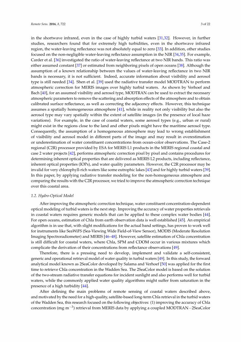
The developed MOD2SEA method combined two lookup tables (LUTs) from 2SeaColor andMODTRAN as schematically shown in Figure 3.

Remote Sens. 2016, 8, 722 6 of 22

3. Methodology

The accuracy of the coupled MOD2SEA model in doing atmospheric correction and deriving Chla concentration values was evaluated against ground truth measurements and was compared with C2R results.

3.1. The Coupled MOD2SEA Model

The developed MOD2SEA method combined two lookup tables (LUTs) from 2SeaColor and MODTRAN as schematically shown in Figure 3.

Figure 3. Diagram of the coupled MOD2SEA model (pixel based).

These LUTs were generated by simulating the water-leaving reflectance for varying ranges of the governing biophysical variables (with respect to range of these water quality variables at the NIOZ jetty station (Table 1)) and MODTRAN parameters based on different combinations of visibilities and aerosol models at specific viewing-illumination geometries for every MERIS image separately. Table 1 presents the LUT composition of the 2SeaColor model and the MODTRAN input variables in this assessment.

Table 1. Lookup table composition of MOD2SEA model.

LUT Variables Range Increment Unit Chla 0–150 5; 0.1 mg·m−3 SPM 0–150 5; 0.1 g·m−3

CDOM absorption at 440 nm 0–2.5 1; 0.1 m−1 Visibility 5–50 1 km

Aerosol type Rural, Maritime, Urban - -

Figure 3. Diagram of the coupled MOD2SEA model (pixel based).

These LUTs were generated by simulating the water-leaving reflectance for varying ranges of thegoverning biophysical variables (with respect to range of these water quality variables at the NIOZjetty station (Table 1)) and MODTRAN parameters based on different combinations of visibilitiesand aerosol models at specific viewing-illumination geometries for every MERIS image separately.Table 1 presents the LUT composition of the 2SeaColor model and the MODTRAN input variables inthis assessment.

Table 1. Lookup table composition of MOD2SEA model.

LUT Variables Range Increment Unit

Chla 0–150 5; 0.1 mg·m−3

SPM 0–150 5; 0.1 g·m−3

CDOM absorption at 440 nm 0–2.5 1; 0.1 m−1

Visibility 5–50 1 kmAerosol type Rural, Maritime, Urban - -

Remote Sens. 2016, 8, 722 7 of 22

The details on simulation of RRS by the 2SeaColor model and TOA radiance by the MODTRANradiative transfer code are described as follows:

3.1.1. Reflectance (RRS) Simulation by 2SeaColor Forward Model

The 2SeaColor model is based on the solution of the two-stream radiative transfer equationsincluding direct sunlight, as described by Duntley (1942, 1963) [61,62]. Both the analytical forwardmodel and the inversion scheme are provided in detail in Salama and Verhoef [50]. The reflectanceresult predicted by the 2SeaColor model is r∞

sd, the directional-hemispherical reflectance of thesemi-infinite medium, which is linked to IOPs by Salama and Verhoef [50]:

r∞sd =

√1 + 2x− 1√

1 + 2x + 2µw(1)

where x is the ratio of backscattering to absorption coefficients (x = bb/a), and µw is the cosine of the solarzenith angle beneath the water surface. The reflectance factor r∞

sd can be approximated by Q × R(0−)under sunny conditions, where Q = 3.25 and R(0−) is the irradiance reflectance beneath the surface [63],which can be converted to above-surface remote sensing reflectance (RRS) by Lee et al. [64].

RRS =0.52× R (0−)

1− 1.7× R (0−)(2)

Total absorption and backscattering coefficient of water constituents (a and bb) were calculatedusing Equations (3) and (4) respectively [27,48].

a (λ) = aw (λ) + achl (λ) + anap (λ) + acdom (λ) (3)

bb (λ) = bbw (λ) + bb,chl (λ) + bb,nap (λ) (4)

where the subscripts w, chl, nap and cdom stand for water molecules, chlorophyll, non-algae particlesand colored dissolved organic matter, respectively. As implemented in Salama and Shen [65],the absorption coefficients of the water constituents (a) are parameterized by (Bricaud et al. [66];Lee et al. [67]; Lee et al. [68]). Also, the backscattering coefficients of the water constituents (bb) wereparametrized by (Doxaran et al. [69] and Morel et al. [70]).

Table 2. Summary of the used parameterizations.

Variable Parametrization Equation Reference

Chla absorptionachl (λ) = [a0 (λ) + a1 (λ)× lnachl (443)]× achl (443)achl (443) = 0.06× [Chl]0.65 (5) [68]

CDOM absorption acdom (λ) = acdom (440)× exp [−Scdom (λ− 440)] (6) [66]

Nap absorptionanap (λ) = anap (440)× exp

[−Snap × (λ− 440)

]anap (440) = a∗nap (440)× [SPM]

(7) [67]

Chla backscatteringbb,chl (λ) =

{0.002+ 0.01×

[0.5− 0.25× log10[Cchl

]×

(λ

550

)n]}× bb,chl (550)

bb,chl (550) = 0.416× [Chl]0.766(8) [70]

NAP backscattering bnap (λ) = bnap (550)× ( 550λ )−γ −

[1− tanh

(0.5× γ2)]× anap (λ)

bnap (550) = b∗nap (550)× I × [SPM](9) [69]

Scattering of water molecules bbw (λ); Listed values, Table (3.8), page 104. (10) [71]

Absorption of water molecules aw(λ); Listed values (11) [72]

In Table 2, [Chl], [SPM] and acdom (440) stand for Chla concentration, SPM concentration andthe CDOM absorption at 440 nm respectively. The absorption and backscattering coefficients ofwater molecules (aw and bbw) were taken from previous studies (Mobley [71]; Pope and Fry [72])and a0 and a1 were given in Lee et al. [67]. The initial values of non-algae particle absorption(a∗nap (440) = 0.036 m2·g−1), spectral slope of non-algae particles (Snap = 0.011 nm−1), spectral slope of

Remote Sens. 2016, 8, 722 8 of 22

CDOM (Scdom = 0.013 nm−1) and specific scattering coefficient of non-algae particles (b∗nap (550) = 0.282)were taken from the Hommersom et al. [11] SIOP measurements at 37 stations in the WaddenSea. Also, the initial values of γ and I (γ = 0.6 and I = 0.019) for the North Sea were taken fromDoxaran et al. [69] and Petzold [73], respectively. In this study, we used the 2Seacolor forward modeland the various parameterizations described in Table 2 to simulate the water-leaving reflectance(RRS spectra) values for a series of combinations of Chla, SPM and CDOM concentration (Table 1) andfor the given SZA associated with every MERIS image separately. The simulated values of RRS spectrafor all MERIS bands were stored in a water LUT for the MERIS bands and then used as RRS inputparameters for MODTRAN to calculate the TOA radiances in the MERIS bands.

3.1.2. Top of Atmosphere (TOA) Radiance Simulation by MODTRAN

MODTRAN is the successor of the atmospheric radiative transfer model LOWTRAN [74]. It ispublicly available from the Air Force Research Laboratory in the USA. The latest version of MODTRAN(5.2.1) contains large spectral databases of the extraterrestrial solar irradiance and the absorption ofall relevant atmospheric gases at a high spectral resolution. The accurate calculation of atmosphericmultiple scattering makes it a very appropriate tool for reliable simulation and interpretation of remotesensing problems in the optical and thermal spectral regions [75]. To apply MODTRAN simulations,first of all several parameters describing the real atmospheric conditions should be determined asinputs for this model. Table 3 shows the standard definition of MODTRAN inputs with respect to theranges of average values of atmospheric and geometric variables variation over one image for fouryears of all available MERIS images between 2007 and 2010 over the Dutch part of the Wadden Sea.In the MERIS image, some of the local atmospheric (O3, H2O) and geometric variables (VZA, SZA andRAA) can be used as input for MODTRAN. Note that for every MERIS image a separate input filewas created by establishing the local atmospheric (O3, H2O, CO2) and geometric variables (VZA, SZA,RAA) of that specific run to MODTRAN (Figure 3). These parameters could be retrieved from MERISancillary data per pixel using Matlab.

Table 3. Input parameters for MODTRAN4 simulations.

Parameter Range or Value Unit

Atmospheric profile Mid Latitude Summer -Correlated-k option Yes -

DISORT number of streams 8 -Concentration of CO2 * 380–390 ppm

H2O 0.5–4.5 g·cm−2

O3 250–450 DUSZA 30–80 degreeVZA 5–30 degreeRAA 0–150 degree

Visibility 5–50 (1 km increment) kmAerosol Model Rural, Maritime, Urban -Surface height 0 kmSensor Height 800 km

Molecular band model resolution 1.0 cm−1

Start, ending wavelength −1000 nm

* Annual CO2 concentration level can be in Global Greenhouse Reference Network [76].

In this study, we varied the aerosol type (rural, maritime and urban) and visibility (5 to 50 kmwith 1 km step) and thus made a total of 135 scenarios for each lookup table and given atmosphericstate and angular geometry, which were extracted from the MERIS image ancillary data per image.For each scenario the MODTRAN Interrogation Technique (MIT) was applied by using surface albedosof 0.0, 0.5 and 1.0 (the MIT is explained in detail by Verhoef and Bach [75]). The output .tp7 fileof MODTRAN quantified the TOA radiance spectrum for each simulated wavelength from 350 to

Remote Sens. 2016, 8, 722 9 of 22

1000 nm. Then in the MIT the .tp7 file was used as input to derive three MODTRAN parameters(gain factor (G), path radiance (L0), and spherical albedo (S)). These parameters are spectral variablesdepending on various atmospheric conditions [75]. The spectral response functions (SRF) of the MERISbands were convolved with the MODTRAN parameters to compute L0, G and S for every MERIS bandand these simulations were stored in the atmospheric LUTs (Atmos LUTs MERIS).

3.1.3. The MOD2SEA Retrievals

The simulated TOA radiance of MERIS data in the MODTRAN output file, LTOA (Wm−2·sr−1·µm−1),Can be expressed in surface reflectance r by the following equation [77]:

LTOA = L0 +Gr

1− Sr(12)

where r is the hemispherical reflectance (=π RRS) leaving the water surface, L0 is the total radiance forzero surface albedo (Wm−2·sr−1·µm−1), S is the spherical albedo of the atmosphere and G is the overallgain factor. In this study, the LUTs of water-leaving reflectance generated by the 2SeaColor modelwere used as RRS input parameters of Equation (12) to calculate TOA radiance for all combinations ofwater properties and atmospheric conditions and then organized in a water-atmosphere lookup table(water-atmosphere). The simultaneous retrieval of Chla, SPM, CDOM concentration, aerosol typeand visibility was then performed by spectrally fitting the MOD2SEA-simulated TOA radiances(using RMSE) to MERIS TOA radiances for all MERIS bands except the band numbers 1, 2 and 11.Band 11 is located in the O2-A absorption band and can give erroneous results due to sampling errorsof MERIS. Bands 1 and 2 gave systematic deviations in RRS after atmospheric correction. The causeof this problem is presently still unknown. In this retrieval, Chla retrieval using the coupledMOD2SEA model was performed in two steps. First the increments of 5, 5 and 1 were taken forChla concentration (mg·m−3), SPM concentration (g·m−3) and CDOM absorption at 440 nm (m−1),respectively, to find an approximate solution. Later, in the refined step, the step size of the LUTscomposition was reduced to 0.1 for all water constituents in the identified rough range resultingfrom the first step. Applying this approach led to speeding up the running of the Matlab code and toobtaining more precise results. Although Figure 3 suggests the storage of a fixed LUT for water RRS foreach MERIS image, this LUT was only generated in a loop, and not stored, in order to reduce memoryrequirements. The best fitting combination of water properties and atmospheric conditions was foundduring the generation of the water LUT, but this water LUT was never stored as such, contrary tothe atmospheric LUT, which was actually stored. This approach also allowed greater flexibility byapplying the two-step procedure in finding the best-fitting water properties, by first applying a roughsearch in the first round with large steps in the three concentrations, and in the next round a refinedsearch with small steps over much smaller ranges. It should be noted that the current procedureapplied to a single pixel per matchup date is not suitable to be applied pixel by pixel, and this issue isleft for a future study.

3.2. MERIS Case-2 Regional (C2R) Processor

The Case-2 regional processor (C2R) [42], available in the Basis ERS and ENVISAT (A) ATSRand MERIS Toolbox (BEAM) software, has been widely used to derive water quality parameters fromMERIS images [78–81]. The C2R processor consists of two procedures, one for atmospheric correctionand one for the bio-optical part for retrieving the IOPs of water columns. The Neural Networks (NN)in C2R were trained with Hydrolight [71] simulations and in situ measurements in the German bightand from other cruises in European seas [42]. More details can be found in Doerffer and Schiller [42].The output of the C2R processor, including IOPs: the absorption coefficient of Chla at wavelength443 nm (achl (443)), the absorption coefficient of CDOM (aCDOM (443)), the total absorption (atot (443)),and the scattering coefficient of SPM (bspm (443)) were then used to define water quality parameters

Remote Sens. 2016, 8, 722 10 of 22

such as Chla and SPM. Equations to relate BEAM processor IOPs to water quality concentrations ofChla and SPM are presented as follows:

[Chla] = 21.0× achl (443)1.04 (13)

[SPM] = 1.72× bspm (443) (14)

where [Chl], [SPM], achl (443) and bsmp (443) stand for Chla concentration, SPM concentration, the Chlabsorption at 443 nm and SPM scattering coefficient at 443 nm, respectively.

3.3. Validation

To evaluate the accuracy of the MOD2SEA coupled model and the C2R processor, we appliedthese two models to the 35 matchup moments of MERIS observations and four years of concurrentChla measurements (2007–2010) at the NIOZ jetty location, separately. The validation of modelsimulations were performed in two different levels of atmospheric correction and water retrievalmodels. Since the NIOZ jetty station is located close to the land, for every image, the darkest pixelfrom 5 by 5 pixels around the location of this station was extracted first. By selecting the darkest pixelfrom the 5 × 5 neighborhood centered on the jetty station, we exclude cloudy and land pixels, as wellas water pixels close to the shore that are possibly influenced by an adjacency effect due to the nearland area. Of course an underlying assumption in our approach is that the water of the darkest pixelhas the same composition as found at the location of the jetty station. However, since the water currentis mostly strong near the inlet to the Wadden Sea, we are confident that the water is well-mixed, andlocal gradients in water properties are small.

3.3.1. Atmospheric Correction

The accuracy of atmospheric correction methods using the coupled MOD2SEA model and C2Rprocessor was evaluated against the ground truth water-leaving reflectance for all 35 matchupsbetween 2007 and 2010 at the NIOZ jetty station. Four statistical parameters, the root mean squareerror (RMSE), the determination coefficient (R2), the normalized root mean square error (NRMSE)and relative root mean square error (RRMSE) [82] were used to quantify the goodness-of-fit betweenderived and measured water-leaving reflectance values at the NIOZ jetty data where near-concurrent(±1 h) MERIS measurements were available. To do this, three MERIS bands 3, 5 and 7 were selected.Finally, the accuracy of the proposed MOD2SEA model in doing atmospheric correction was comparedagainst C2R processor products. The results of this assessment are presented in Section 4.2.

3.3.2. Water Model Inversion

The accuracy of retrieved Chla concentration values using the coupled MOD2SEA model andthe C2R processor were evaluated against ground truth Chla measurements for all 35 matchup pointsat the NIOZ jetty station between 2007 and 2010. The results of this evaluation are presented inSection 4.3. It should be mentioned that in view of the main objective of this study (retrieval ofChla concentration) and the availability of ground truth measurements, investigation of changes inother water constituents (SPM and CDOM concentration) was considered to fall outside of the scope ofthis study, although these were retrieved along with Chla using MOD2SEA. In addition, the visibilityand aerosol type were retrieved simultaneously with water quality parameter concentration whichwere used in the model to simulate water-leaving reflectance values based on the best matching TOAradiance by MOD2SEA coupled model.

4. Results

4.1. Variability of MODTRAN Parameters (L0, G and S) at Different Atmospheric Conditions

The case of the three aerosol types—rural, maritime and urban—for a visibility of 20 km on7 October 2007 was used as an example to display the result of applying MODTRAN to the MERIS

Remote Sens. 2016, 8, 722 11 of 22

bands for three atmospheric conditions. We used MIT method [75] to derive L0, G and S values usingsurface albedos of 0.0, 0.5 and 1.0 for the mentioned visibilities and aerosol types in these figures.

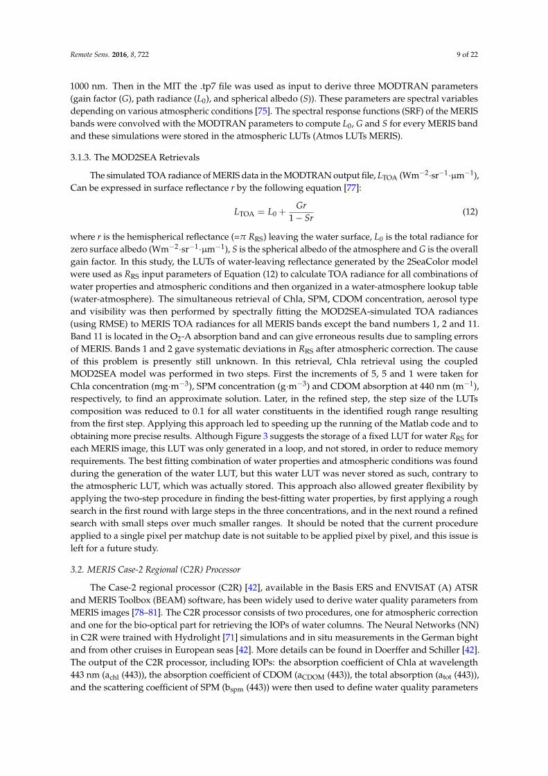
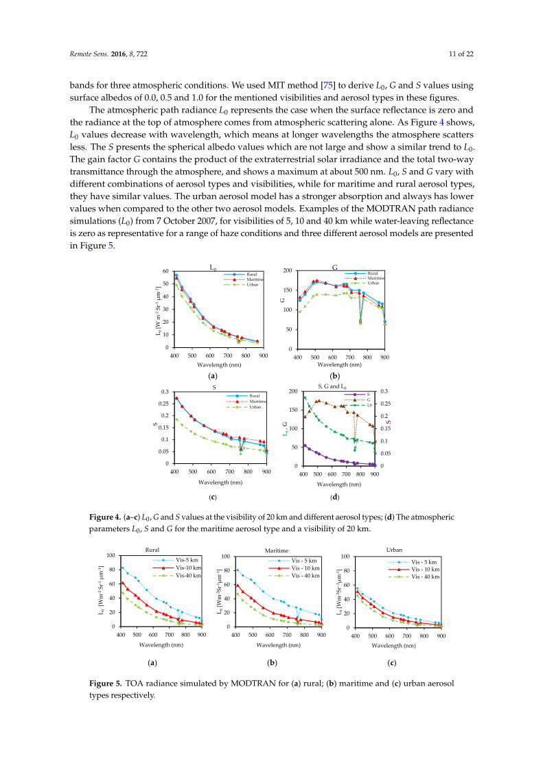
The atmospheric path radiance L0 represents the case when the surface reflectance is zero andthe radiance at the top of atmosphere comes from atmospheric scattering alone. As Figure 4 shows,L0 values decrease with wavelength, which means at longer wavelengths the atmosphere scattersless. The S presents the spherical albedo values which are not large and show a similar trend to L0.The gain factor G contains the product of the extraterrestrial solar irradiance and the total two-waytransmittance through the atmosphere, and shows a maximum at about 500 nm. L0, S and G vary withdifferent combinations of aerosol types and visibilities, while for maritime and rural aerosol types,they have similar values. The urban aerosol model has a stronger absorption and always has lowervalues when compared to the other two aerosol models. Examples of the MODTRAN path radiancesimulations (L0) from 7 October 2007, for visibilities of 5, 10 and 40 km while water-leaving reflectanceis zero as representative for a range of haze conditions and three different aerosol models are presentedin Figure 5.

Remote Sens. 2016, 8, 722 11 of 22

bands for three atmospheric conditions. We used MIT method [75] to derive L0, G and S values using surface albedos of 0.0, 0.5 and 1.0 for the mentioned visibilities and aerosol types in these figures.

The atmospheric path radiance L0 represents the case when the surface reflectance is zero and the radiance at the top of atmosphere comes from atmospheric scattering alone. As Figure 4 shows, L0 values decrease with wavelength, which means at longer wavelengths the atmosphere scatters less. The S presents the spherical albedo values which are not large and show a similar trend to L0. The gain factor G contains the product of the extraterrestrial solar irradiance and the total two-way transmittance through the atmosphere, and shows a maximum at about 500 nm. L0, S and G vary with different combinations of aerosol types and visibilities, while for maritime and rural aerosol types, they have similar values. The urban aerosol model has a stronger absorption and always has lower values when compared to the other two aerosol models. Examples of the MODTRAN path radiance simulations (L0) from 7 October 2007, for visibilities of 5, 10 and 40 km while water-leaving reflectance is zero as representative for a range of haze conditions and three different aerosol models are presented in Figure 5.

(a) (b)

(c) (d)

Figure 4. (a–c) L0, G and S values at the visibility of 20 km and different aerosol types; (d) The atmospheric parameters L0, S and G for the maritime aerosol type and a visibility of 20 km.

(a) (b) (c)

0

20

40

60

80

100

400 500 600 700 800 900

L 0[W

m-2

Sr-1

µm-1

]

Wavelength (nm)

Maritime

Vis - 5 kmVis - 10 kmVis - 40 km

0

20

40

60

80

100

400 500 600 700 800 900

L 0[W

m-2

Sr--1

µm-1

]

Wavelength (nm)

Urban

Vis - 5 kmVis - 10 kmVis - 40 km

0

50

100

150

200

400 500 600 700 800 900

G

Wavelength (nm)

GRuralMaritimeUrban

0

0.05

0.1

0.15

0.2

0.25

0.3

400 500 600 700 800 900

S

Wavelength (nm)

SRuralMaritimeUrban

0

0.05

0.1

0.15

0.2

0.25

0.3

0

50

100

150

200

400 500 600 700 800 900

S

L 0,G

Wavelength (nm)

S, G and L0SGL0

0

10

20

30

40

50

60

400 500 600 700 800 900

L 0[W

m-2

Sr-1

µm-1

]

Wavelength (nm)

L0RuralMaritimeUrban

0

20

40

60

80

100

400 500 600 700 800 900

L 0[W

m-2

Sr-1

µm-1

]

Wavelength (nm)

Rural

Vis-5 kmVis-10 kmVis-40 km

Figure 4. (a–c) L0, G and S values at the visibility of 20 km and different aerosol types; (d) The atmosphericparameters L0, S and G for the maritime aerosol type and a visibility of 20 km.

Remote Sens. 2016, 8, 722 11 of 22

bands for three atmospheric conditions. We used MIT method [75] to derive L0, G and S values using surface albedos of 0.0, 0.5 and 1.0 for the mentioned visibilities and aerosol types in these figures.

The atmospheric path radiance L0 represents the case when the surface reflectance is zero and the radiance at the top of atmosphere comes from atmospheric scattering alone. As Figure 4 shows, L0 values decrease with wavelength, which means at longer wavelengths the atmosphere scatters less. The S presents the spherical albedo values which are not large and show a similar trend to L0. The gain factor G contains the product of the extraterrestrial solar irradiance and the total two-way transmittance through the atmosphere, and shows a maximum at about 500 nm. L0, S and G vary with different combinations of aerosol types and visibilities, while for maritime and rural aerosol types, they have similar values. The urban aerosol model has a stronger absorption and always has lower values when compared to the other two aerosol models. Examples of the MODTRAN path radiance simulations (L0) from 7 October 2007, for visibilities of 5, 10 and 40 km while water-leaving reflectance is zero as representative for a range of haze conditions and three different aerosol models are presented in Figure 5.

(a) (b)

(c) (d)

Figure 4. (a–c) L0, G and S values at the visibility of 20 km and different aerosol types; (d) The atmospheric parameters L0, S and G for the maritime aerosol type and a visibility of 20 km.

(a) (b) (c)

0

20

40

60

80

100

400 500 600 700 800 900

L 0[W

m-2

Sr-1

µm-1

]

Wavelength (nm)

Maritime

Vis - 5 kmVis - 10 kmVis - 40 km

0

20

40

60

80

100

400 500 600 700 800 900

L 0[W

m-2

Sr--1

µm-1

]

Wavelength (nm)

Urban

Vis - 5 kmVis - 10 kmVis - 40 km

0

50

100

150

200

400 500 600 700 800 900

G

Wavelength (nm)

GRuralMaritimeUrban

0

0.05

0.1

0.15

0.2

0.25

0.3

400 500 600 700 800 900

S

Wavelength (nm)

SRuralMaritimeUrban

0

0.05

0.1

0.15

0.2

0.25

0.3

0

50

100

150

200

400 500 600 700 800 900

S

L 0,G

Wavelength (nm)

S, G and L0SGL0

0

10

20

30

40

50

60

400 500 600 700 800 900

L 0[W

m-2

Sr-1

µm-1

]

Wavelength (nm)

L0RuralMaritimeUrban

0

20

40

60

80

100

400 500 600 700 800 900

L 0[W

m-2

Sr-1

µm-1

]

Wavelength (nm)

Rural

Vis-5 kmVis-10 kmVis-40 km

Figure 5. TOA radiance simulated by MODTRAN for (a) rural; (b) maritime and (c) urban aerosoltypes respectively.

Remote Sens. 2016, 8, 722 12 of 22

As this figure shows, the calculated TOA radiances for the urban aerosol type show a lower rangeof variation compared to the maritime and rural cases. All the values of TOA radiance for the urbanaerosol type are between 0 and 60 (Wm−2·sr−1·µm−1), while these values for maritime and ruralones vary between 0 and 80 (Wm−2·sr−1·µm−1). On the other hand, the simulated TOA radiances byMODTRAN differ significantly not only with aerosol type, but also with visibility. Lower visibilitygives higher TOA radiances. Consequently, a wrong assumption about visibility or aerosol type leadsto a wrong calculation of water-leaving reflectance and as a result the water parameter concentrationsmay be overestimated or underestimated.

4.2. Atmospheric Correction Validation

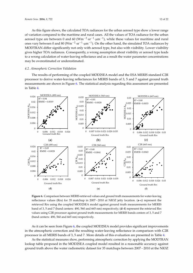
The results of performing of the coupled MOD2SEA model and the ESA MERIS standard C2Rprocessor to derive water-leaving reflectances for MERIS bands of 3, 5 and 7 against ground truthmeasurements are shown in Figure 6. The statistical analysis regarding this assessment are presentedin Table 4.

Remote Sens. 2016, 8, 722 12 of 22

Figure 5. TOA radiance simulated by MODTRAN for (a) rural; (b) maritime and (c) urban aerosol types respectively.

As this figure shows, the calculated TOA radiances for the urban aerosol type show a lower range of variation compared to the maritime and rural cases. All the values of TOA radiance for the urban aerosol type are between 0 and 60 (Wm−2·sr−1·µm−1), while these values for maritime and rural ones vary between 0 and 80 (Wm−2·sr−1·µm−1). On the other hand, the simulated TOA radiances by MODTRAN differ significantly not only with aerosol type, but also with visibility. Lower visibility gives higher TOA radiances. Consequently, a wrong assumption about visibility or aerosol type leads to a wrong calculation of water-leaving reflectance and as a result the water parameter concentrations may be overestimated or underestimated.

4.2. Atmospheric Correction Validation

The results of performing of the coupled MOD2SEA model and the ESA MERIS standard C2R processor to derive water-leaving reflectances for MERIS bands of 3, 5 and 7 against ground truth measurements are shown in Figure 6. The statistical analysis regarding this assessment are presented in Table 4.

(a) (b) (c)

(d) (e) (f)

Figure 6. Comparison between MERIS-retrieved values and ground truth measurements for water-leaving reflectance values (Rrs) for 35 matchup in 2007−2010 at NIOZ jetty location. (a–c) represent the retrieved Rrs using the coupled MOD2SEA model against ground truth measurements for MERIS band of 3, 5 and 7 (band centers: 490, 560 and 665 nm) respectively; (d–f) represent the retrieved Rrs values using C2R processor against ground truth measurements for MERIS bands centers of 3, 5 and 7 (band centers: 490, 560 and 665 nm) respectively.

As it can be seen from Figure 6, the coupled MOD2SEA model provides significant improvements in the atmospheric correction and the resulting water-leaving reflectance in comparison with C2R processor in all MERIS bands of 3, 5 and 7. More details of this evaluation are presented in Table 4.

0

0.004

0.008

0.012

0.016

0.02

0.024

0 0.006 0.012 0.018 0.024

MO

D2S

EA R

RS

Ground truth Rrs

MOD2SEA (490 nm)R2 = 0.84RMSE = 0.0019

0

0.005

0.01

0.015

0.02

0.025

0.03

0.035

0 0.007 0.014 0.021 0.028 0.035

MO

D2S

EA R

RS

Ground truth Rrs

MOD2SEA (560 nm)R2 = 0.81RMSE = 0.0028

0

0.005

0.01

0.015

0.02

0.025

0.03

0.035

0 0.007 0.014 0.021 0.028 0.035

C2R

RRS

Ground truth Rrs

C2R (560 nm)

R2 = 0.68RMSE = 0.0041

0

0.005

0.01

0.015

0.02

0.025

0.03

0 0.006 0.012 0.018 0.024 0.03

MO

D2S

EA R

RS

Ground truth Rrs

MOD2SEA (665 nm)

R2 = 0.80RMSE= 0.0033

0

0.005

0.01

0.015

0.02

0.025

0.03

0 0.006 0.012 0.018 0.024 0.03

C2R

RRS

Ground truth Rrs

C2R (665 nm)

R2 = 0.62RMSE= 0.0043

0

0.004

0.008

0.012

0.016

0.02

0.024

0 0.006 0.012 0.018 0.024

C2R

RRS

Ground truth Rrs

C2R (490 nm)R2 = 0.69RMSE = 0.0028

Figure 6. Comparison between MERIS-retrieved values and ground truth measurements for water-leavingreflectance values (Rrs) for 35 matchup in 2007−2010 at NIOZ jetty location. (a–c) represent theretrieved Rrs using the coupled MOD2SEA model against ground truth measurements for MERISband of 3, 5 and 7 (band centers: 490, 560 and 665 nm) respectively; (d–f) represent the retrieved Rrsvalues using C2R processor against ground truth measurements for MERIS bands centers of 3, 5 and 7(band centers: 490, 560 and 665 nm) respectively.

As it can be seen from Figure 6, the coupled MOD2SEA model provides significant improvementsin the atmospheric correction and the resulting water-leaving reflectance in comparison with C2Rprocessor in all MERIS bands of 3, 5 and 7. More details of this evaluation are presented in Table 4.

As the statistical measures show, performing atmospheric correction by applying the MODTRANlookup table proposed in the MOD2SEA coupled model resulted in a reasonable accuracy againstground truth above the water radiometric dataset for 35 matchups between 2007−2010 at the NIOZ

Remote Sens. 2016, 8, 722 13 of 22

jetty station for bands 3, 5 and 7 respectively. In addition, the MOD2SEA coupled model showssignificant improvement especially in band 3 with R2 = 0.84, RMSE = 0.0022, NRMSE = 13.18% andRRMSE = 21.08% in comparison with C2R. The standard C2R processor also shows higher accuracyfor band 3 (R2 = 0.69, RMSE = 0.0047) in comparison with bands 5 (R2 = 0.68, RMSE = 0.0058) and7 (R2 = 0.62, RMSE = 0.0063), respectively.

Table 4. Models’ performance evaluation in atmospheric correction part.

Statistical Measures R2 RMSE NRMSE (%) RRMSE (%)

MERIS bands/Model MOD2SEA C2R MODSEA C2R MOD2SEA C2R MOD2SEA C2R

3 0.84 0.69 0.0022 0.0047 13.18 28.03 21.08 44.815 0.81 0.68 0.0034 0.0058 14.38 24.20 20.07 33.787 0.80 0.62 0.0035 0.0063 14.39 25.51 30.94 54.87

4.3. Water Retrieval Validation

The comparisons of C2R and MOD2SEA Chla retrieval against ground truth measurements areshown in Figure 7 and related statistical analysis are presented in Table 5.

Remote Sens. 2016, 8, 722 13 of 22

As the statistical measures show, performing atmospheric correction by applying the MODTRAN lookup table proposed in the MOD2SEA coupled model resulted in a reasonable accuracy against ground truth above the water radiometric dataset for 35 matchups between 2007−2010 at the NIOZ jetty station for bands 3, 5 and 7 respectively. In addition, the MOD2SEA coupled model shows significant improvement especially in band 3 with R2 = 0.84, RMSE = 0.0022, NRMSE = 13.18% and RRMSE = 21.08% in comparison with C2R. The standard C2R processor also shows higher accuracy for band 3 (R2 = 0.69, RMSE = 0.0047) in comparison with bands 5 (R2 = 0.68, RMSE = 0.0058) and 7 (R2 = 0.62, RMSE = 0.0063), respectively.

Table 4. Models’ performance evaluation in atmospheric correction part.

Statistical Measures R2 RMSE NRMSE (%) RRMSE (%)MERIS bands/Model MOD2SEA C2R MODSEA C2R MOD2SEA C2R MOD2SEA C2R

3 0.84 0.69 0.0022 0.0047 13.18 28.03 21.08 44.81 5 0.81 0.68 0.0034 0.0058 14.38 24.20 20.07 33.78 7 0.80 0.62 0.0035 0.0063 14.39 25.51 30.94 54.87

4.2. Water Retrieval Validation

The comparisons of C2R and MOD2SEA Chla retrieval against ground truth measurements are shown in Figure 7 and related statistical analysis are presented in Table 5.

(a)

(b)

Figure 7. Comparison between MERIS-derived and measured log Chla (mg·m−3) for 35 matchup moments. (a) MOD2SEA and (b) C2R.

Assessing the model accuracy using R2 and RMSE shows the reasonable agreement between the measured and retrieved Chla (mg·m−3) for all the matchup points during 2007–2010 at the NIOZ jetty location with a significant regression (Figure 7: R2 = 0.88 and RMSE = 3.32 mg·m−3) during the period of four years. In addition, the comparison of this model with the C2R processor shows significant improvement in retrieval of Chla. The result of this comparison is presented in Table 5.

Table 5. Models performance evaluation Chla retrieval.

There are several possible reasons for the improvement of MOD2SEA in the retrieval of Chla in comparison with the C2R procedure, but the most obvious one is probably that the SIOPs used in the training of the C2R neural network might be more generic and thus different from the ones used in this study and which are more applicable to the Wadden Sea. In addition, the derived Chla data for 35 matchups between 2007–2010 by the MOD2SEA coupled model was examined to see how well the ground truth values (mg·m−3) agreed with those derived from the MERIS images (mg·m−3) at the

0.1

1

10

100

0.1 1 10 100

Log

(der

ived

Chl

a)

Log (ground truth Chla)

MOD2SEAR2= 0.88RMSE= 3.32

0.1

1

10

100

0.1 1 10 100

Log

(der

ived

Chl

a)

Log (ground truth Chla)

C2RR2 = 0.17RMSE = 4.46

Statistical Measures R2 RMSE NRMSE (%) RRMSE (%) MOD2SEA 0.88 3.32 15.25 53.31

C2R 0.17 4.42 20.30 70.98

Figure 7. Comparison between MERIS-derived and measured log Chla (mg·m−3) for 35 matchupmoments. (a) MOD2SEA and (b) C2R.

Assessing the model accuracy using R2 and RMSE shows the reasonable agreement between themeasured and retrieved Chla (mg·m−3) for all the matchup points during 2007–2010 at the NIOZ jettylocation with a significant regression (Figure 7: R2 = 0.88 and RMSE = 3.32 mg·m−3) during the periodof four years. In addition, the comparison of this model with the C2R processor shows significantimprovement in retrieval of Chla. The result of this comparison is presented in Table 5.

Table 5. Models performance evaluation Chla retrieval.

Statistical Measures R2 RMSE NRMSE (%) RRMSE (%)

MOD2SEA 0.88 3.32 15.25 53.31C2R 0.17 4.42 20.30 70.98

There are several possible reasons for the improvement of MOD2SEA in the retrieval of Chla incomparison with the C2R procedure, but the most obvious one is probably that the SIOPs used in thetraining of the C2R neural network might be more generic and thus different from the ones used inthis study and which are more applicable to the Wadden Sea. In addition, the derived Chla data for35 matchups between 2007–2010 by the MOD2SEA coupled model was examined to see how well theground truth values (mg·m−3) agreed with those derived from the MERIS images (mg·m−3) at theNIOZ jetty location (Figure 8). In this figure, the X-axis presents the date while the Y-axis presents the

Remote Sens. 2016, 8, 722 14 of 22

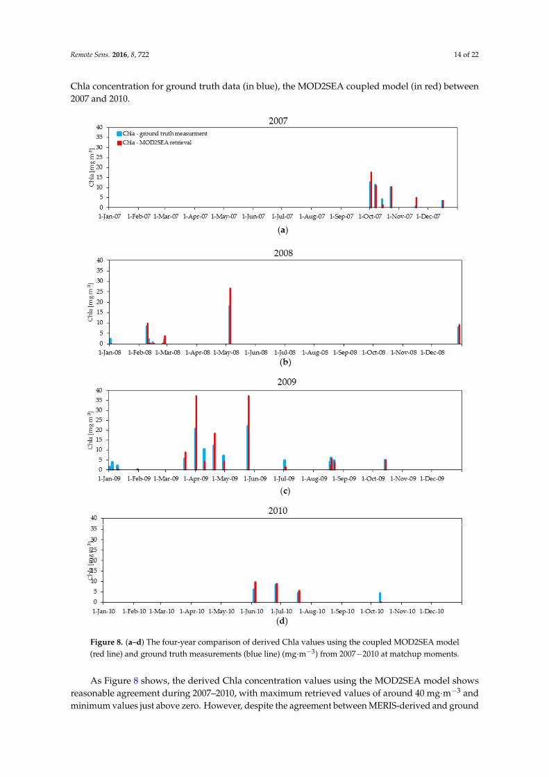
Chla concentration for ground truth data (in blue), the MOD2SEA coupled model (in red) between2007 and 2010.

Remote Sens. 2016, 8, 722 14 of 22

NIOZ jetty location (Figure 8). In this figure, the X-axis presents the date while the Y-axis presents the Chla concentration for ground truth data (in blue), the MOD2SEA coupled model (in red) between 2007 and 2010.

Figure 8. (a–d) The four-year comparison of derived Chla values using the coupled MOD2SEA model (red line) and ground truth measurements (blue line) (mg·m−3) from 2007−2010 at matchup moments.

As Figure 8 shows, the derived Chla concentration values using the MOD2SEA model shows reasonable agreement during 2007–2010, with maximum retrieved values of around 40 mg·m−3 and minimum values just above zero. However, despite the agreement between MERIS-derived and

Figure 8. (a–d) The four-year comparison of derived Chla values using the coupled MOD2SEA model(red line) and ground truth measurements (blue line) (mg·m−3) from 2007−2010 at matchup moments.

As Figure 8 shows, the derived Chla concentration values using the MOD2SEA model showsreasonable agreement during 2007–2010, with maximum retrieved values of around 40 mg·m−3 andminimum values just above zero. However, despite the agreement between MERIS-derived and ground

Remote Sens. 2016, 8, 722 15 of 22

truth Chla in a four-year period, systematic overestimations at high Chla concentration values (duringApril and May) mg·m−3 were also identified. Chla products, particularly during the phytoplanktonbloom seasons of spring and summer, require further development. This overestimation might beexplained by the Chla parametrization of the Lee et al. [68] model, since it appears that the Chla modelcalibration based on that model does not fit that well for the Wadden Sea. This Chla overestimationusing satellite images was also in agreement with a Chla retrieval overestimation in most of theEuropean seas studies by Zibordi et al. [58].

5. Discussion

Accurate estimation of water-leaving reflectance from satellite sensors is a fundamental goal forocean color satellite missions [83]. Basically, the commonly applied atmospheric correction methodsbased on zero water-leaving reflectance in the near-infrared bands fail when applied to turbid waterssince the high concentrations of water constituents lead to a detectable water-leaving reflectance in thenear-infrared region in satellite image. In this study, we focused on the long-term retrieval of Chlaconcentration from MERIS images in the Wadden Sea, and the MOD2SEA coupled model is proposedas a tool to improve the retrieval of Chla concentration from earth observation data in this area.

Calculating accurate water-leaving reflectance spectra in order to translate them into Chlaconcentration under different atmospheric conditions is a crucial part of this study, since the atmosphere,in most cases, contributes more than 90% of the TOA radiance signal [41]. We can attribute the successof the MOD2SEA coupled model to its capability of combining simulations from 2SeaColor withthe MODTRAN radiative transfer model for different combinations of aerosol type, visibility andwater constituent concentrations for all MERIS bands to simulate TOA radiances, instead of applyingroutine atmospheric correction and water retrieval algorithms separately. Furthermore, based ona heterogeneous atmosphere assumption of the coupled MOD2SEA model, this technique can helpsuppress the influence of local haze variations in satellite images. Thus, applying this method resultsin a considerable improvement of the accuracy of the atmospheric correction, which is the mostproblematic part of remote sensing data processing for turbid waters like the Wadden Sea.

However, satellite estimation of Chla concentration is still difficult for coastal waters, where Chla,SPM and CDOM occur in various mixtures which complicate the derivation of their concentrationsfrom reflectance observations. The 2SeaColor model performed well while the commonly appliedwater quality algorithms might fail in water constituent retrieval. Figure 9 shows an example ofcoupled MOD2SEA model spectral matchings for 2 October 2007.

As this figure shows, good matches are found between modelled and observed TOA radiance aswell as modelled and atmospherically corrected water-leaving reflectance with respect to identifiedvisibility and aerosol type by the coupled model. All in all, assessing the MOD2SEA Chla retrievalsfrom MERIS data at one location (NIOZ jetty station) for a period of four years (2007–2010) showsreasonable agreement with ground truth measurements (R2 = 0.88, RMSE = 33.2%). The 33.2% RMSEappears reasonable enough, as compared with the validation of the SeaWiFS Chla data product forglobal open ocean waters with a relative RMSE of about 58% [1]. In addition, this model showsconsiderable improvement to retrieve Chla concentration from satellite images in comparison withsimilar studies for the Wadden Sea [10,18]. The results of retrieved Chla concentration using thiscoupled model are within the range of measured Chla concentration (mg·m−3) on the ground reportedby other researchers, while a clear seasonal pattern is observed with the peak values during spring(in May). For example, Hommersom [10] reported Chla concentration range variations in the WaddenSea during eight surface water sampling campaigns in 2006−2007 in 156 stations while Chla alsoshowed a strong seasonal pattern with the highest values during spring in May. Chang et al. [84]showed the higher Chla concentrations occurred in May. Reuter et al. [85] provided continuous dataon Chla concentration of the Wadden Sea at a time series station established in autumn 2002 bythe University of Oldenburg. They reported a clear seasonal pattern in Chla concentration between2007–2008 which has the highest values in May and the lowest values in November. Tillman et al. [86]

Remote Sens. 2016, 8, 722 16 of 22

showed a large variability of Chla concentration over the year in the Wadden Sea. Winter concentrationswere much lower than summer concentrations while in spring a phytoplankton bloom with peakconcentrations occurs. Cadée and Hegeman [87] showed that yearly patterns of Chla concentrationwere similar in the Wadden Sea, although the overall inter-annual variability is large, as well as themaxima measured during spring bloom (in May). All in all, regarding the reasonable agreement of theMOD2SEA results with ground truth measurements and considering the turbid nature and complexheterogeneity in the turbid Wadden Sea, the performance of this coupled model should be regarded asencouraging and satisfactory enough.

Remote Sens. 2016, 8, 722 16 of 22

much lower than summer concentrations while in spring a phytoplankton bloom with peak concentrations occurs. Cadée and Hegeman [87] showed that yearly patterns of Chla concentration were similar in the Wadden Sea, although the overall inter-annual variability is large, as well as the maxima measured during spring bloom (in May). All in all, regarding the reasonable agreement of the MOD2SEA results with ground truth measurements and considering the turbid nature and complex heterogeneity in the turbid Wadden Sea, the performance of this coupled model should be regarded as encouraging and satisfactory enough.

(a)

(b)

(c)

(d)

Figure 9. (a) The best match identified by the coupled model between simulated TOA radiances vs. pixel TOA radiance; (b) Spectral differences between observed and simulated TOA radiance; (c) The simulated RRS (extracted from the best TOA radiance match) vs. the simulated 2SeaColor RRS; (d) Spectral differences between simulated RRS by 2SeaColor and atmospherically corrected RRS from observed TOA radiance by MOD2SEA.

It is also worth mentioning that in shallow coastal waters like the Wadden Sea the bottom might influence the reflected signal to the sensor. This is not the case for the NIOZ jetty data where, due to the depth of >5 m and the high turbidity of the water (Table 1) near the NIOZ jetty and the surrounding area, the bottom effect on observed reflectance is negligible. This has been confirmed in the quality check of the NIOZ jetty data and the corresponding MERIS pixels. However, in the other shallower parts of the Wadden Sea, the bottom effect might contribute substantially in the visible region of the spectrum. As can be seen in Figure 1, the effect of the bottom is visible in large areas of the Wadden Sea satellite image. Thus, for shallow waters it is recommended in future studies to develop water constituent retrieval algorithms by incorporating sea bottom effects in the hydro-optical model. We speculate that developing a hydro-optical model including the bottom effect may lead to significant improvements in the derived water constituent concentrations from earth observation data in this shallow coastal region. That is why, in the next phase of this research, we are going to include the bottom effect contribution into the TOA radiance calculation to derive and provide Chla concentration maps over the Wadden Sea.

-2

-1.5

-1

-0.5

0

0.5

1

1.5

2

480 550 620 690 760 830 900

Spec

tral

Diff

eren

ces

Wavelength (nm)

TOA Spectral differences

0

0.004

0.008

0.012

0.016

480 550 620 690 760 830 900

R RS

Wavelength (nm)

Atmosphericlly corrected RRS ve 2Sea color RRS

Rrs - retrieved from TOAradianceRrs - modeled

-0.01

-0.005

0

0.005

0.01

480 550 620 690 760 830 900

Spec

tral

Diff

eren

ces

Wavelength (nm)

RRS Spectral differences

0

10

20

30

40

50

60

480 550 620 690 760 830 900

TOA

[Wm

-2 S

r -1 µ

m-1

]

Wavelength (nm)

Pixel TOA vs simulated MOD2SEA TOA

TOA - observedTOA - modeled

Figure 9. (a) The best match identified by the coupled model between simulated TOA radiancesvs. pixel TOA radiance; (b) Spectral differences between observed and simulated TOA radiance;(c) The simulated RRS (extracted from the best TOA radiance match) vs. the simulated 2SeaColor RRS;(d) Spectral differences between simulated RRS by 2SeaColor and atmospherically corrected RRS fromobserved TOA radiance by MOD2SEA.

It is also worth mentioning that in shallow coastal waters like the Wadden Sea the bottom mightinfluence the reflected signal to the sensor. This is not the case for the NIOZ jetty data where, due to thedepth of >5 m and the high turbidity of the water (Table 1) near the NIOZ jetty and the surroundingarea, the bottom effect on observed reflectance is negligible. This has been confirmed in the qualitycheck of the NIOZ jetty data and the corresponding MERIS pixels. However, in the other shallowerparts of the Wadden Sea, the bottom effect might contribute substantially in the visible region ofthe spectrum. As can be seen in Figure 1, the effect of the bottom is visible in large areas of theWadden Sea satellite image. Thus, for shallow waters it is recommended in future studies to developwater constituent retrieval algorithms by incorporating sea bottom effects in the hydro-optical model.We speculate that developing a hydro-optical model including the bottom effect may lead to significantimprovements in the derived water constituent concentrations from earth observation data in this

Remote Sens. 2016, 8, 722 17 of 22

shallow coastal region. That is why, in the next phase of this research, we are going to include thebottom effect contribution into the TOA radiance calculation to derive and provide Chla concentrationmaps over the Wadden Sea.

For the Wadden Sea, and many other estuaries, knowledge of local specific inherent opticalproperties to locally calibrate retrieval algorithms is often lacking, and more research is still needed.For the Wadden Sea, Peters et al. [88] reported a complete set of SIOPs for Chla, SPM and CDOMmeasurements. However, the data of Peters were all collected at one location (the Marsdiep inlet)and only for two days (in May 2000). After that, the only published set of SIOP measurements inthe Wadden Sea was constructed by Hommersom et al. [11]. Using Hommersom’s measurements,SIOPs increased the accuracy of the derived Chla concentration significantly in comparison to previousefforts in this region. However, Hommersom’s measurements lack seasonal information on the SIOPswhile there is currently not much information on the SIOPs to be the basis for a hydro-optical modelfor the Wadden Sea. Without any doubt, having seasonal SIOPs may lead to an improved accuracy ofretrieved Chla using this coupled model. Thus, more in situ data (especially on SIOPs) is still necessaryfor the model calibration.

Although our current efforts are centered on validating the proposed coupledatmospheric-hydroptical model in the highly turbid Wadden Sea using MERIS satellite images, it isunclear how broadly applicable this coupled model will be and to what extent these findings couldbe generalized. Thus, we suggest to extend this study to other parts of the world using variousocean color remote sensors. However, to apply this method to other regions, first the availability ofvalid SIOPs (water quality constituent’s absorption and backscattering coefficient), in addition to theaccurate ecological and geophysical knowledge of the interest area (i.e., the ranges of water constituentconcentrations) are needed. Furthermore, spectral response functions of the desired sensor as wellas atmospheric parameters and illumination geometry of the satellite image to run MODTRAN arerequired. As a consequence, access to accurate in situ water-leaving reflectance and water qualityparameter concentration is essential for the assessment of primary data products from satellite oceancolor missions [55] using the proposed approach.

The water Framework Directive regulations from the European Union force member states tomonitor all their coastal areas (Environment Directorate-General of the European Commission, 2000).Availability of one decade of MERIS images (2002–2012) over the Wadden Sea, gives the opportunityto provide long-term Chla distribution maps using this coupled model with reasonable accuracyand to conduct a one-decade phenological analysis in this area. To provide Chla concentration mapswith reasonable accuracy, the proposed method should be applied pixel by pixel for the wholeregion of interest. To speed up the pixel-based approach, a filter can be introduced to remove thosecombinations of visibilities and aerosol types from the MODTRAN lookup table which result innegative water-leaving reflectance values in any band, by considering the recorded TOA signalper pixel. On the other hand, other water quality parameters like SPM and CDOM as well asvisibility and aerosol model maps can be produced as output of the MOD2SEA code. Of particularinterest when analyzing the variability in the MERIS-derived Chla data trend for the Wadden Sea iswhether any significant decreasing trend from 2002–2012 would indicate the effect of prior nutrientreduction management actions. This has significant implications for identifying positive anomalyevents and may act as an alert for management actions. Clearly, climatic variability needs to beconsidered carefully when interpreting the long-term data trends and when making managementdecisions [1]. Furthermore, this established MERIS-based Chla data record may serve as baselinedata to continuously monitor the estuary’s eutrophic state, and the validated algorithm may extendsuch observations to the future using various satellite continuity missions. The Ocean Land ColorInstrument (OLCI), embedded on the Sentinel-3 platform, is a sensor especially adapted for aquaticremote sensing [89] and succeeded the MERIS sensor in 2015 [90]. The launch of Sentinel-3 and OLCIwill secure future consistent operational monitoring by medium resolution data for water qualityassessment also of coastal zones and bays [89]. OLCI is designed mainly for global biological and

Remote Sens. 2016, 8, 722 18 of 22

biochemical oceanography, which constrains its spatial resolution. On the other hand, the asymmetricview of OLCI will offer sun-glint free images in 21 spectral bands (from ultraviolet to near-infraredwavelengths) with an improved spatial coverage and temporal frequency. OLCI will provide highquality optical ocean observations (e.g., normalized water-leaving radiance, inherent optical properties,spectral attenuation of downwelling irradiance, photosynthetically active radiation, particle sizedistribution) and allow more accurate retrieval of the ocean color variables (e.g., Chlorophyll, SPM andCDOM concentrations) [91] where the OLCI bands are optimized to measure ocean color over openocean and coastal zones. Sentinel-3 was successfully launched in February 2016 and will give freeaccess to satellite data of the Wadden Sea. It is expected that the MOD2SEA coupled model will alsooperate successfully to derive Chla concentration using OLCI images for highly turbid waters andthat it will result in an accuracy improvement in atmospheric correction and Chla retrieval aspects incomparison with the MERIS sensor. Thus, applying this method for further studies using OLCI dataover the Wadden Sea is recommended.

6. Conclusions

A coupled atmospheric-hydro-optical model (MOD2SEA) has been proposed and validated toderive long-term Chla concentration (mg·m−3), visibility and aerosol type from MERIS observationsfor the coastal turbid area of the Wadden Sea. At one location, the model validation showed a goodagreement between MERIS-derived and measured Chla concentration for a period of four years(2007–2010). We attribute the success of this approach to the simultaneous retrieval of atmosphere andwater properties. In addition, we have found that water and atmospheric properties have differenteffects on TOA radiance spectra and therefore these are separately retrievable from MERIS data ifthe coupled MOD2SEA model is used. Using this coupled atmospheric-hydro-optical model led toconsiderable improvement for the simultaneous retrieval of water and atmosphere properties usingearth observation data, with significant results in the accuracy in comparison with other algorithmsapplied to derive Chla in the Wadden Sea.

Acknowledgments: The authors would like to thank three anonymous reviewers for their constructive commentsand suggestions to improve the quality of our paper. We also would like to thank the European Space Agency forproviding the MERIS data within the framework of the “Integrated Network for Production and Loss Assessmentin the Coastal Environment (IN PLACE)” project, which is funded by NWO-ZKO.

Author Contributions: All authors have made major and unique contributions in this research. The satellite datafrom ESA archive of MERIS images was provided by Suhyb Salama (as a part of IN PLACE project). Ground truthmeasurements from NIOZ jetty station were provided by Marcel Wernand. The Matlab code was written byBehnaz Arabi and Suhyb Salama and was then modified and extended by Wouter Verhoef. Behnaz Arabiperformed in situ RRS (λ), Chla and MERIS imagery categorization, matchup points finding, MODTRAN andmodel simulations, data analysis as well as the results interpretation. The original manuscript was written byBehnaz Arabi. In addition, Wouter Verhoef and Suhyb Salama supervised the research and discussed the resultsand provided substantial contribution in revising the manuscript at all stages. All co-authors participated in theimprovement of the manuscript. All authors have read and approved the final version of this manuscript.

Conflicts of Interest: The authors declare no conflict of interest.

References

1. Le, C.; Hu, C.; English, D.; Cannizzaro, J.; Chen, Z.; Feng, L.; Boler, R.; Kovach, C. Towards a long-termchlorophyll-a data record in a turbid estuary using MODIS observations. Prog. Oceanogr. 2013, 109, 90–103.[CrossRef]

2. Casal, G.; Furey, T.; Dabrowski, T.; Nolan, G. Generating a Long-Term Series of Sst and Chlorophyll-a for theCoast of Ireland. ISPRS Int. Arch. Photogramm. Remote Sens. Spat. Inf. Sci. 2015, XL-7/W3, 933–940. [CrossRef]

3. Werdell, P.J.; Bailey, S.W.; Franz, B.A.; Harding, L.W.; Feldman, G.C.; McClain, C.R. Regional andseasonal variability of chlorophyll-a in Chesapeake Bay as observed by SeaWiFS and MODIS-Aqua.Remote Sens. Environ. 2009, 113, 1319–1330. [CrossRef]

4. Moradi, M.; Kabiri, K. Spatio-temporal variability of SST and Chlorophyll-a from MODIS data in the PersianGulf. Mar. Pollut. Bull. 2015, 98, 14–25. [CrossRef] [PubMed]

Remote Sens. 2016, 8, 722 19 of 22

5. Peters, S.W.M.; Woerd, H.; Van der Pasterkamp, R. CHL maps of the Dutch coastal zone: A case study withinthe REVAMP project. Structure 2004, 2003, 10–13.

6. Van der Woerd, H.; Pasterkamp, R.; Van der Woerd, H.; Pasterkamp, R. Mapping the North Sea turbidcoastal waters using SeaWIFS data. Can. J. Remote Sens. 2004, 30, 44–53. [CrossRef]

7. Le, C.; Hu, C.; English, D.; Cannizzaro, J.; Kovach, C. Climate-driven chlorophyll-a changes in a turbidestuary: Observations from satellites and implications for management. Remote Sens. Environ. 2013, 130,11–24. [CrossRef]

8. Mélin, F.; Vantrepotte, V.; Clerici, M.; D’Alimonte, D.; Zibordi, G.; Berthon, J.-F.; Canuti, E.Multi-sensor satellite time series of optical properties and chlorophyll-a concentration in the AdriaticSea. Prog. Oceanogr. 2011, 91, 229–244. [CrossRef]

9. Hommersom, A.; Wernand, M.R.; Peters, S.; De Boer, J. A review on substances and processes relevant foroptical remote sensing of extremely turbid marine areas, with a focus on the Wadden Sea. Helgol. Mar. Res.2010, 64, 75–92. [CrossRef]

10. Hommersom, A. ”Dense water” and “Fluid Sand” Optical Properties and Methods for Remote Sensing of theEstremely Turbid Wadden Sea. Ph.D. Thesis, Vrije University Amsterdam, Amsterdam, The Netherlands, 2010.

11. Hommersom, A.; Peters, S.; Wernand, M.R.; de Boer, J. Spatial and temporal variability in bio-opticalproperties of the Wadden Sea. Estuar. Coast. Shelf Sci. 2009, 83, 360–370. [CrossRef]

12. Philippart, C.J.M.; Salama, M.S.; Kromkamp, J.C.; van der Woerd, H.J.; Zuur, A.F.; Cadée, G.C. Four decadesof variability in turbidity in the western Wadden Sea as derived from corrected Secchi disk readings.J. Sea Res. 2013, 82, 67–79. [CrossRef]

13. Poremba, K.; Tillmann, U.; Hesse, K.-J. Distribution patterns of bacterioplankton and chlorophyll-a in theGerman Wadden Sea. Helgol. Mar. Res. 1999, 53, 28–35. [CrossRef]

14. Philippart, C.J.M.; Beukema, J.J.; Cadée, G.C.; Dekker, R.; Goedhart, P.W.; Van Iperen, J.M.; Leopold, M.F.;Herman, P.M.J. Impacts of nutrient reduction on coastal communities. Ecosystems 2007, 10, 95–118. [CrossRef]

15. Gemein, N.; Stanev, E.; Brink-spalink, G.; Wolff, J.-O.; Reuter, R. Patterns of suspended matter in the EastFrisian Wadden Sea: Comparison of numerical simulations with MERIS observations. Eur. Assoc. RemoteSens. Lab. Proc. 2006, 5, 180–198.

16. Bartholdy, J.; Folving, S. Sediment classification and surface type mapping in the Danish Wadden Sea byremote sensing. Neth. J. Sea Res. 1986, 20, 337–345. [CrossRef]

17. Hommersom, A.; Researcher, I. A case study on the use of hydropt in the wadden sea. In Proceedings of the2nd MERIS (A) ATSR User Workshop, Frascati, Italy, 22–26 September 2008.

18. Hommersom, A.; Peters, S.; Woerd, H.J.; Van der Eleveld, M.A. Tracking wadden sea water masses withan inverse bio-optical and endmember model satellite data. EARSeL Proc. 2010, 9, 1–12.

19. Schroeder, T.; Behnert, I.; Schaale, M.; Fischer, J.; Doerffer, R. Atmospheric correction algorithm for MERISabove case-2 waters. Int. J. Remote Sens. 2007, 28, 1469–1486. [CrossRef]

20. Gordon, H.R.; Wang, M. Retrieval of water-leaving radiance and aerosol optical thickness over the oceanswith SeaWiFS: A preliminary algorithm. Appl. Opt. 1994, 33, 443–452. [CrossRef] [PubMed]

21. Goyens, C.; Jamet, C.; Schroeder, T. Evaluation of four atmospheric correction algorithms for MODIS-Aquaimages over contrasted coastal waters. Remote Sens. Environ. 2013, 131, 63–75. [CrossRef]

22. Jamet, C.; Loisel, H.; Kuchinke, C.P.; Ruddick, K.; Zibordi, G.; Feng, H. Comparison of threeSeaWiFS atmospheric correction algorithms for turbid waters using AERONET-OC measurements.Remote Sens. Environ. 2011, 115, 1955–1965. [CrossRef]

23. Siegel, D.A.; Wang, M.; Maritorena, S.; Robinson, W. Atmospheric correction of satellite ocean color imagery:the black pixel assumption. Appl. Opt. 2000, 39, 3582–3591. [CrossRef] [PubMed]

24. Carpintero, M.; Polo, M.J.; Salama, M.S. Simultaneous atmospheric correction and quantification ofsuspended particulate matter in the Guadalquivir estuary from Landsat images. Proc. Int. Assoc. Hydrol. Sci.2015, 368, 15–20. [CrossRef]

25. Mélin, F.; Zibordi, G.; Berthon, J.-F. Assessment of satellite ocean color products at a coastal site.Remote Sens. Environ. 2007, 110, 192–215. [CrossRef]

26. Santer, R.; Schmechtig, C. Adjacency effects on water surfaces: Primary scattering approximation andsensitivity study. Appl. Opt. 2000, 39, 361–375. [CrossRef] [PubMed]

27. Sathyendranath, S. International ocean-colour coordinating group remote sensing of ocean colour in coastal,and other optically-complex. Waters 2000, 3, 2–11.

Remote Sens. 2016, 8, 722 20 of 22

28. Hu, C.; Carder, K.L.; Muller-Karger, F.E. Atmospheric correction of SeaWiFS imagery over turbid coastalwaters: A practical method. Remote Sens. Environ. 2000, 74, 195–206. [CrossRef]

29. Wang, M.; Shi, W. The NIR-SWIR combined atmospheric correction approach for MODIS ocean color dataprocessing. Opt. Express 2007, 15, 15722–15733. [CrossRef] [PubMed]

30. Ruddick, K.G.; De Cauwer, V.; Park, Y.-J.; Moore, G.F. Seaborne measurements of near infrared water-leavingreflectance: The similarity spectrum for turbid waters. Limnol. Oceanogr. 2006, 51, 1167–1179. [CrossRef]

31. Wang, M. Remote sensing of the ocean contributions from ultraviolet to near-infrared using the shortwaveinfrared bands: Simulations. Appl. Opt. 2007, 46, 1535–1547. [CrossRef] [PubMed]

32. Wang, M.; Shi, W. Estimation of ocean contribution at the MODIS near-infrared wavelengths along the eastcoast of the U.S.: Two case studies. Geophys. Res. Lett. 2005, 32, 1–5. [CrossRef]

33. Wang, M.; Shi, W.; Tang, J. Water property monitoring and assessment for China’s inland Lake Taihu fromMODIS-Aqua measurements. Remote Sens. Environ. 2011, 115, 841–854. [CrossRef]

34. Salama, M.S.; Shen, F. Simultaneous atmospheric correction and quantification of suspended particulatematters from orbital and geostationary earth observation sensors. Estuar. Coast. Shelf Sci. 2010, 86, 499–511.[CrossRef]

35. Doxaran, D.; Lamquin, N.; Park, Y.-J.; Mazeran, C.; Ryu, J.-H.; Wang, M.; Poteau, A. Retrieval of the seawaterreflectance for suspended solids monitoring in the East China Sea using MODIS, MERIS and GOCI satellitedata. Remote Sens. Environ. 2014, 146, 36–48. [CrossRef]

36. Carder, K.L.; Cattrall, C.; Chen, F.R. MODIS clear water epsilons (ATBD 21). Ocean. Color. Web. 2002, 2002,1–4.

37. Gould, R.W.; Arnone, R.A.; Martinolich, P.M. Spectral dependence of the scattering coefficient in case 1 andcase 2 waters. Appl. Opt. 1999, 38, 2377–2383. [CrossRef] [PubMed]

38. Ruddick, K.G.; Ovidio, F.; Rijkeboer, M. Atmospheric correction of SeaWiFS imagery for turbid coastal andinland waters. Appl. Opt. 2000, 39, 897–912. [CrossRef] [PubMed]

39. Shen, F.; Verhoef, W.; Zhou, Y.X.; Salama, M.S.; Liu, X.L. Satellite estimates of wide-range suspendedsediment concentrations in Changjiang (Yangtze) estuary using MERIS data. Estuar. Coasts 2010, 33,1420–1429. [CrossRef]

40. Verhoef, W.; Bach, H. Coupled soil-leaf-canopy and atmosphere radiative transfer modeling to simulatehyperspectral multi-angular surface reflectance and TOA radiance data. Remote Sens. Environ. 2007, 109,166–182. [CrossRef]

41. Shen, F.; Verhoef, W. Suppression of local haze variations in MERIS images over turbid coastal waters forretrieval of suspended sediment concentration. Opt. Express 2010, 18, 12653–12662. [CrossRef] [PubMed]

42. Doerffer, R.; Schiller, H. The MERIS Case 2 water algorithm. Int. J. Remote Sens. 2007, 28, 517–535. [CrossRef]43. Duan, H.; Ma, R.; Simis, S.G.H.; Zhang, Y. Validation of MERIS case-2 water products in Lake Taihu, China.

GIScience Remote Sens. 2012, 49, 873–894. [CrossRef]44. Salama, M.S. Roadmap Waterkwaliteit: Helder Beeld op Troebel Water; ITC: Boston, MA, USA, 2014.45. O’Reilly, J.E.; Maritorena, S.; Mitchell, B.G.; Siegel, D.A.; Carder, K.L.; Garver, S.A.; Kahru, M.; McClain, C.

Ocean color chlorophyll algorithms for SeaWiFS. J. Geophys. Res. 1998, 103, 24937. [CrossRef]46. O’Reilly, J.; Maritorena, S. Ocean color chlorophyll a algorithms for SeaWiFS, OC2, and OC4: Version 4.

In SeaWiFS Postlaunch Calibration and Validation Analyses; NASA: Washington, DC, USA, 2000; pp. 8–22.47. Dasgupta, S.; Singh, R.P.; Kafatos, M. Comparison of global chlorophyll concentrations using MODIS data.

Adv. Space Res. 2009, 43, 1090–1100. [CrossRef]48. Arnone, R.; Babin, M.; Barnard, A.H.; Boss, E.; Cannizzaro, J.P.; Carder, K.L.; Chen, F.R.; Devred, E.;

Doerffer, R.; Du, K.; et al. Remote Sensing of Inherent Optical Properties: Fundamentals, Tests of Algorithms,and Applications; The International Ocean-Colour Coordinating Group: Dartmouth, NH, Canada, 2006.

49. Salama, M.S.; Radwan, M.; van der Velde, R. A hydro-optical model for deriving water quality variables fromsatellite images (HydroSat): A case study of the Nile River demonstrating the future Sentinel-2 capabilities.Phys. Chem. Earth 2012, 50–52, 224–232. [CrossRef]

50. Salama, M.S.; Verhoef, W. Two-stream remote sensing model for water quality mapping: 2SeaColor.Remote Sens. Environ. 2014, 157, 111–122. [CrossRef]

51. Ridderinkhof, H.; Zimmerman, J.T.F.; Philippart, M.E. Tidal exchange between the North Sea and DutchWadden Sea and mixing time scales of the tidal basins. Neth. J. Sea Res. 1990, 25, 331–350. [CrossRef]

Remote Sens. 2016, 8, 722 21 of 22

52. Zibordi, G.; Berthon, J.F.; Mélin, F.; D’Alimonte, D. Cross-site consistent in situ measurements for satelliteocean color applications: The BiOMaP radiometric dataset. Remote Sens. Environ. 2011, 115, 2104–2115.[CrossRef]

53. Wernand, M.R.; Poseidon, S. Paintbox Historical Archives of Ocean Colour in Global-Change Poseidon’sVerfdoos. Ph.D. Thesis, Utrecht University, Utrecht, The Netherlands, 2011.

54. Ly, J.; Philippart, C.J.M.; Kromkamp, J.C. Phosphorus limitation during a phytoplankton spring bloom in thewestern Dutch Wadden Sea. J. Sea Res. 2014, 88, 109–120. [CrossRef]

55. Zibordi, G.; Berthon, J.F.; Mélin, F.; D’Alimonte, D.; Kaitala, S. Validation of satellite ocean color primaryproducts at optically complex coastal sites: Northern Adriatic Sea, Northern Baltic Proper and Gulf ofFinland. Remote Sens. Environ. 2009, 113, 2574–2591. [CrossRef]

56. Schroeder, T.; Schaale, M.; Fischer, J. Retrieval of atmospheric and oceanic properties from MERISmeasurements: A new Case-2 water processor for BEAM. Int. J. Remote Sens. 2007, 28, 5627–5632. [CrossRef]

57. Peters, S.W.M.; Eleveld, M.; Pasterkamp, R.; Van Der Woerd, H.; Devolder, M.; Jans, S.; Park, Y.; Ruddick, K.;Block, T.; Brockmann, C.; et al. Atlas of Chlorophyll-a Concentration for the North; Sea Based on MERIS Imagery of2003; Vrije Universiteit: Amsterdam, The Netherlands, 2005.

58. Zibordi, G.; Mélin, F.; Berthon, J.F.; Canuti, E. Assessment of MERIS ocean color data products for Europeanseas. Ocean Sci. 2013, 9, 521–533. [CrossRef]

59. Zibordi, G.; Mélin, F.; Berthon, J.F. Comparison of SeaWiFS, MODIS and MERIS radiometric products ata coastal site. Geophys. Res. Lett. 2006, 33, 1–4. [CrossRef]

60. Loisel, H.; Vantrepotte, V.; Jamet, C.; Dat, D.N. Challenges and new advances in ocean color remote sensingof coastal waters. In Oceanography Research; In Tech: Greer, SC, USA, 2013.

61. Duntley, S.Q. The optical properties of diffusing materials. J. Opt. Soc. Am. 1942, 32, 61–70. [CrossRef]62. Duntley, S.Q. Light in the sea. J. Opt. Soc. Am. 1963, 53, 214–233. [CrossRef]63. Morel, A.; Gentili, B. Diffuse reflectance of oceanic waters. II Bidirectional aspects. Appl. Opt. 1993, 32,

6864–6879. [CrossRef] [PubMed]64. Lee, Z.; Carder, K.L.; Arnone, R.A. Deriving inherent optical properties from water color: A multiband

quasi-analytical algorithm for optically deep waters. Appl. Opt. 2002, 41, 5755–5772. [CrossRef] [PubMed]65. Salama, M.S.; Shen, F. Stochastic inversion of ocean color data using the cross-entropy method. Opt. Express

2010, 18, 479–499. [CrossRef] [PubMed]66. Briucaud, A.; Morel, A.; Prieur, L. Absorption by dissolved organic matter of the sea (yellow substance) in

the UV and visible domains. Limnol. Oceanogr. 1981, 26, 43–53. [CrossRef]67. Lee, Z.; Carder, K.L.; Mobley, C.D.; Steward, R.G.; Patch, J.S. Hyperspectral remote sensing for shallow

waters. I. A semianalytical model. Appl. Opt. 1998, 37, 6329–6338. [CrossRef] [PubMed]68. Lee, Z.; Carder, K.L.; Mobley, C.D.; Steward, R.G.; Patch, J.S. Hyperspectral remote sensing for shallow

waters. 2. Deriving bottom depths and water properties by optimization. Appl. Opt. 1999, 38, 3831–3843.[CrossRef] [PubMed]

69. Doxaran, D.; Ruddick, K.; McKee, D.; Gentili, B.; Tailliez, D.; Chami, M.; Babin, M. Spectral variations oflight scattering by marine particles in coastal waters, from visible to near infrared. Limnol. Oceanogr. 2009,54, 1257–1271. [CrossRef]

70. Morel, A.; Maritorena, S. Bio-optical properties of oceanic waters: A reappraisal. J. Geophys. Res. 2001, 106,7163–7180. [CrossRef]

71. Mobley, C.D. Light and Water: Radiative Transfer in Natural Waters; Academic Press: Cambridge, MA,USA, 1994.

72. Pope, R.M.; Fry, E.S. Absorption spectrum (380–700 nm) of pure water. II. Integrating cavity measurements.Appl. Opt. 1997, 36, 8710–8723. [CrossRef] [PubMed]

73. Petzold, T. Volume Scattering Functions for Selected Ocean Waters; No. SIO-REF-72-78; Scripps Institution ofOceanography La Jolla Ca Visibility Laboratory: San Diego, CA, USA, 1972.

74. Kneizys, F.X.; Shettle, E.P.; Abreu, L.W.; Chetwynd, J.H.; Anderson, G.P. Users Guide to LOWTRAN 7;No. AFGL-TR-88-0177; Air Force Geophysics Lab Hanscom: Bedford, MA, USA, 1988.

75. Verhoef, W.; Bach, H. Simulation of hyperspectral and directional radiance images using coupled biophysicaland atmospheric radiative transfer models. Remote Sens. Environ. 2003, 87, 23–41. [CrossRef]

76. Global Greenhouse Reference Network 2017. Available online: http://www.esrl.noaa.gov/gmd/ccgg/trends/ (accessed on 31 August 2016).

Remote Sens. 2016, 8, 722 22 of 22

77. Berk, A.; Anderson, G.P.; Acharya, P.K.; Shettle, E.P. MODTRAN 5.2. 1 User’s Manual; Spectral Sciences Inc.:Burlington, MA, USA, 2011.

78. Attila, J.; Koponen, S.; Kallio, K.; Lindfors, A.; Kaitala, S.; Ylöstalo, P. MERIS Case II water processorcomparison on coastal sites of the northern Baltic Sea. Remote Sens. Environ. 2013, 128, 138–149. [CrossRef]

79. Beltrán-Abaunza, J.M.; Kratzer, S.; Brockmann, C. Evaluation of MERIS products from Baltic Sea coastalwaters rich in CDOM. Ocean Sci. 2014, 10, 377–396. [CrossRef]

80. Smith, M.E.; Bernard, S.; O’Donoghue, S. The assessment of optimal {MERIS} ocean colour products in theshelf waters of the KwaZulu-Natal Bight, South Africa. Remote Sens. Environ. 2013, 137, 124–138. [CrossRef]

81. Ambarwulan, W.; Verhoef, W.; Mannaerts, C.M.; Salama, M.S. Estimating total suspended matterconcentration in tropica coastal waters of the Berau estuary, Indonesia. Int. J. Remote Sens. 2012, 33,4919–4936. [CrossRef]

82. Bayat, B.; Van der Tol, C.; Verhoef, W. Remote sensing of grass response to drought stress using spectroscopictechniques and canopy reflectance model inversion. Remote Sens. 2016, 8. [CrossRef]

83. Zibordi, G.; Ruddick, K.; Ansko, I.; Moore, G.; Kratzer, S.; Icely, J.; Reinart, A. In situ determination of theremote sensing reflectance: An inter-comparison. Ocean Sci. 2012, 8, 567–586. [CrossRef]

84. Chang, T.S.; Joerdel, O.; Flemming, B.W.; Bartholomä, A. The role of particle aggregation/disaggregationin muddy sediment dynamics and seasonal sediment turnover in a back-barrier tidal basin, East FrisianWadden Sea, southern North Sea. Mar. Geol. 2006, 235, 49–61. [CrossRef]

85. Reuter, R.; Badewien, T.H.; BartholomÄ, A.; Braun, A.; Lübben, A.; Rullkötter, J. A hydrographic time seriesstation in the Wadden Sea (southern North Sea). Ocean Dyn. 2009, 59, 195–211. [CrossRef]

86. Tillmann, U.; Hesse, K.-J.; Colijn, F. Planktonic primary production in the German Wadden Sea.J. Plankton Res. 2000, 22, 1253–1276. [CrossRef]

87. Cadée, G.C. Accumulation and sedimentation of Phaeocystis globosa in the Dutch Wadden Sea. J. Sea Res.1996, 36, 321–327. [CrossRef]

88. Peters, S.W.M. MERIMON-2000: MERIS for Water Quality Monitoring in the Belgian-Dutch-German Coastal Zone;Food and Agriculture Organization of the United Nations: Rome, Italy, 2001.

89. Harvey, E.T.; Kratzer, S.; Philipson, P. Satellite-based water quality monitoring for improved spatial andtemporal retrieval of chlorophyll-a in coastal waters. Remote Sens. Environ. 2014, 158, 417–430. [CrossRef]

90. Saulquin, B.; Fablet, R.; Bourg, L.; Mercier, G.; d’Andon, O.F. MEETC2: Ocean color atmospheric correctionsin coastal complex waters using a Bayesian latent class model and potential for the incoming sentinel 3-OLCImission. Remote Sens. Environ. 2016, 172, 39–49. [CrossRef]

91. Malenovský, Z.; Rott, H.; Cihlar, J.; Schaepman, M.E.; García-Santos, G.; Fernandes, R.; Berger, M.Sentinels for science: Potential of Sentinel-1, -2, and -3 missions for scientific observations of ocean,cryosphere, and land. Remote Sens. Environ. 2012, 120, 91–101.

© 2016 by the authors; licensee MDPI, Basel, Switzerland. This article is an open accessarticle distributed under the terms and conditions of the Creative Commons Attribution(CC-BY) license (http://creativecommons.org/licenses/by/4.0/).