Modal logic for preference based on reasons

Daniel Osherson1 and Scott Weinstein2

1 Princeton University, Princeton NJ 08544, USA,osherson@princeton.edu

2 University of Pennsylvania, Philadelphia PA 19104, USA,weinstein@cis.upenn.edu

Abstract. We discuss the logic of preferences, introducing modal connectives that reflectreasons to prefer that one formula rather than another be true. An axiomatic analysis oftwo such logics is presented.

1 Introduction

The second author is grateful for the opportunity to contribute to this volume in honor ofPeter Buneman, whose colleagueship he enjoyed for many years at Penn. Peter’s passionate andpowerful intellect, his generosity, and his kindness have enriched the lives of all who workedwith him. We dedicate this chapter to him. Our hope is that he, or one among his legionof distinguished students, find something here which they can elaborate in ways beyond ourcapacity to imagine.

The present paper focusses on the modal logic of preference, following up earlier work(Osherson and Weinstein, 2012) on the interaction between preference and reasons. An examplemay help to communicate the kind of situation under investigation. You are deciding whether toadopt a certain dog, Fido; alternatively, you might choose the cat Thomasina. To make up yourmind, you first imagine how life would be with Fido, taking into account the companionship andsafety he would provide but also the expense and bother. Then you do the same for Thomasina.You observe that, compared to Thomasina, life with Fido would have greater value along thefirst two dimensions (companionship and safety) but entail less with respect to the second pair(expense and bother). Somehow, you aggregate these four considerations, and plump for Fido.

Our formal reconstruction of this episode is as follows. The world you live in is one ofmany possibilities including some in which “I adopt Fido” is true and others in which “I adoptThomasina” is true. In choosing between the two plans, you imagine a world rather similar toyours except that the Fido sentence is true, and another world for the Thomasina sentence.These two worlds are compared for the amount of companionship they provide as well as forsafety, expense and bother. A scheme for combining these comparisons is applied, which yieldsyour decision.

The Fido world was delivered by a selection function applied to your current world underthe thought of adopting Fido, and similarly for the Thomasina world. In other words, selectionmakes a choice among possible worlds that satisfy whatever proposition is being entertained.

In the most basic logic, no conditions regulate how the function operates. But stronger theoriesimpose requirements that fill out the idea that selection seeks a world “close” to its startingpoint among the worlds that satisfy the target proposition. The most elementary constraint isreflexivity, which requires that if the starting world satisfies a proposition A, then that worldbe selected when seeking an A-world. A more consequential constraint is that selection beinterpreted metrically, in the sense that the chosen world be uniquely nearest to the startingpoint among A-worlds, for some underlying metric that situates all the worlds in play. Severalconstraints are investigated in Osherson and Weinstein (2012).

The basic logic will be presented shortly, followed by an alternative version that dispenseswith selection. It will be seen that the two systems validate the same formulas, a fact notavailable in Osherson and Weinstein (2012). We then proceed to extend the basic logic inanother direction, by introducing quantifiers. Before getting started, let us acknowledge someof the prior literature on the logic of preference.

Contemporary work includes several systems that elucidate the interaction between choiceand epistemic possibility (see Lang et al., 2003; van Benthem et al., 2009 for an overview). Liu(2008, Ch. 3) is particularly pertinent since it introduces “priorities,” which function somewhatlike reasons in our theory. Liu’s approach is nonetheless different from the one described be-low inasmuch as selection is absent. A different perspective on the integration of preferencesis embodied in the graph-theoretic approach offered in Andreka et al. (2002); different graphsrepresent different orderings of the alternatives in play, and can be conceived as separate rea-sons for choice among them. Within another tradition, multi-attribute utility theory (Keeneyand Raiffa, 1993) analyses the aggregation of reasons by combining utilities based on separatedimensions. The theory reveals the conditions under which aggregation can proceed additivelybut stops short of exploring the logical structure of reasons and preference, as we shall do here.Finally (in this abbreviated review), Dietrich and List (2009) provide a representation theoremrelating choice to the respective bundles of reasons that apply to the available choices; the simpleaxioms invoked for their theorem clarify several issues relating to combining reasons.

We shall not attempt to further summarize the extensive literature on the logic of preference.An excellent review up to 1989 is offered by Hansson (1989). Surveys of later work are availablein Liu (2008) and Dietrich and List (2009). It is, however, worth emphasizing that the formalismspresented below share many features with earlier work. For example, Hansson (1989) introducesa selection function for choosing worlds relevant to an affirmation of preference; a somewhatdifferent kind of selection function (based on the analysis of counterfactuals in Stalnaker, 1968)is central to our own theory. Similarly, the idea of attaching values to possible worlds in orderto analyze preference among statements appears in several works (e.g., Rescher, 1967), and ispivotal here as well. Our approach thus builds on many earlier discussions; but (so far as wecan see) it puts familiar pieces together in a novel way.

2 The basic theory

Turning to our own proposal, we first introduce the family of languages that are used to expresspreferences, then provide their semantics.

2.1 Syntax

Signatures. A given language is determined by its signature, which consists of

(a) a non-empty set P of propositional variables, and(b) a nonempty collection S of nonempty subsets of N (the set 0, 1, . . . of natural numbers).

The elements of S serve as indexes for utility functions.

The numbers appearing in X ∈ S represent specific reasons for preference such as the desire forcompanionship in our introductory example. A set X of reasons influences preference throughaggregation of its members. If

⋃S ∈ S then preference according to

⋃S amounts to preference

tout court ; for, such preference takes into account all reasons in play.

Formulas. The language determined by signature (P,S) is denoted L(P,S), and is built fromthe following symbols.

(a) the set P of propositional variables(b) the unary connective ¬(c) the binary connective ∧(d) for every set X ∈ S, the binary connective X

(e) the two parentheses

Formulas are defined inductively via:

p ∈ P | ¬ϕ | (ϕ ∧ ψ) | (ϕ X ψ) for X ∈ S.

We rely on obvious abbreviations for the boolean connectives including the constants >, ⊥.We also write: (ϕ X ψ) for (ϕ X ψ) ∧ ¬(ψ X ϕ), (ϕ ≈X ψ) for (ϕ X ψ) ∧ (ψ X ϕ),(ϕ X ψ) for (ψ X ϕ), and (ϕ ≺X ψ) for (ψ X ϕ).

To illustrate a formula with modal embedding, suppose that utility indexes refer to commer-cial agents like businesses. Then in a domain that represents economic conditions (availability ofraw materials, tax laws, etc.), ϕ i ψ might mean that ϕ is more conducive to the profitabilityof business i than is ψ. Due to competition (e.g., for scarce resources or market share), i mightbe better off if j does not benefit from the same economic situations as i, yielding, for example:

(ϕ i ψ) → ((ϕ j ψ) ≺i (ψ j ϕ)).

A similar interpretation concerns the fitness of species i, j in a given ecological environment.

2.2 Semantics

According to the semantics provided below, ϕ 1 ψ can be understood as follows. As a functionof the world you actually inhabit, a world w satisfying ϕ, and a world v satisfying ψ are selected.

The formula is true just in case u1(w) > u1(v), where u1 is a utility function from worlds tonumbers, with index 1. Let ϕ,ψ express the adoption of Fido and Thomasina, respectively. Ifthe indexes 1 . . . 4 measure companionship, safety, expense, and bother then X = 1 . . . 4 isthe aggregate index for all four together. So, if w is the world in which Fido is adopted, and vis the world for Thomasina then Fido is your choice if uX(w) > uX(v), in which case ϕ X ψis true at the world you inhabit.

Models. A model for signature (P,S) is based on a nonempty set of points called “worlds.”Subsets of worlds are termed propositions. As discussed above, given a nonempty proposition Aand world w, we pick an alternative to w among the worlds in A. (If w ∈ A then the “alternative”might be w itself.) Such choices are formalized as follows.

(1) Definition: A selection function s over a set W of worlds is a mapping from W×A ⊆W | A 6= ∅ to W such that for all w ∈W and ∅ 6= A ⊆W, s(w,A) ∈ A.

Intuitively, s chooses a member of A that is similar to w.

Next, recall that each world can be evaluated according to different utility scales, indexedby members of S.

(2) Definition: A utility function u over W and S is a mapping from W × S to < (thereals).

For w ∈W and i, X ∈ S, we write u(w, i) as ui(w), and u(w,X) as uX(w).

In a given signature (P,S), P is a nonempty set of propositional variables. The last compo-nent of a model is the assignment of a proposition to each variable in P.

(3) Definition: A truth-assignment (over W and P) is a mapping from P to the power setof W.

For a truth-assignment t, the idea is that p ∈ P is true in w ∈W just in case w ∈ t(p).

(4) Definition: A (basic) model for a signature (P,S) is a quadruple (W, s, u, t) where(a) W is a nonempty set of worlds;(b) s is a selection function over W;(c) u is a utility function over W and S;(d) t is a truth-assignment over W and P.

Propositions. We may now specify the proposition (set of worlds) expressed by a givenformula ϕ in a model M. This proposition is denoted ϕ[M ], and defined as follows.

(5) Definition: Let signature (P,S), ϕ ∈ L(P,S), and model M = (W, s, u, t) for (P,S)be given.

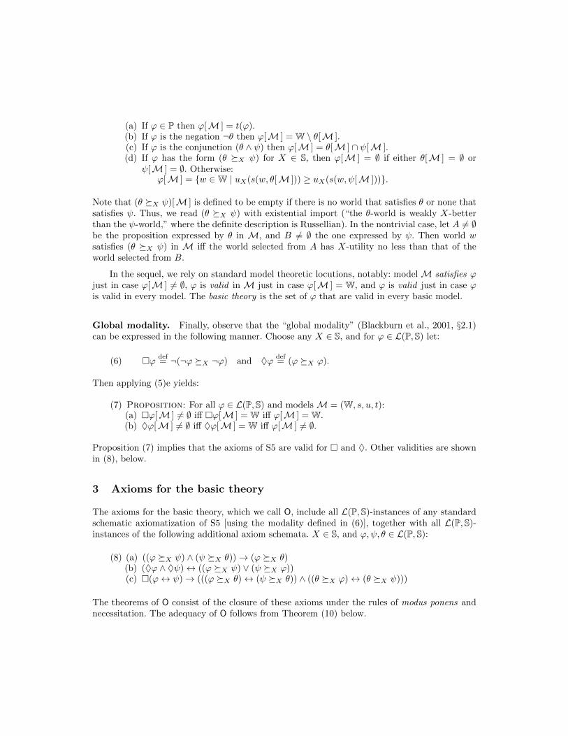
(a) If ϕ ∈ P then ϕ[M ] = t(ϕ).(b) If ϕ is the negation ¬θ then ϕ[M ] = W \ θ[M ].(c) If ϕ is the conjunction (θ ∧ ψ) then ϕ[M ] = θ[M ] ∩ ψ[M ].(d) If ϕ has the form (θ X ψ) for X ∈ S, then ϕ[M ] = ∅ if either θ[M ] = ∅ or

ψ[M ] = ∅. Otherwise:ϕ[M ] = w ∈W | uX(s(w, θ[M ])) ≥ uX(s(w,ψ[M ])).

Note that (θ X ψ)[M ] is defined to be empty if there is no world that satisfies θ or none thatsatisfies ψ. Thus, we read (θ X ψ) with existential import (“the θ-world is weakly X-betterthan the ψ-world,” where the definite description is Russellian). In the nontrivial case, let A 6= ∅be the proposition expressed by θ in M, and B 6= ∅ the one expressed by ψ. Then world wsatisfies (θ X ψ) in M iff the world selected from A has X-utility no less than that of theworld selected from B.

In the sequel, we rely on standard model theoretic locutions, notably: model M satisfies ϕjust in case ϕ[M ] 6= ∅, ϕ is valid in M just in case ϕ[M ] = W, and ϕ is valid just in case ϕis valid in every model. The basic theory is the set of ϕ that are valid in every basic model.

Global modality. Finally, observe that the “global modality” (Blackburn et al., 2001, §2.1)can be expressed in the following manner. Choose any X ∈ S, and for ϕ ∈ L(P,S) let:

(6) ϕdef= ¬(¬ϕ X ¬ϕ) and ♦ϕ

def= (ϕ X ϕ).

Then applying (5)e yields:

(7) Proposition: For all ϕ ∈ L(P,S) and models M = (W, s, u, t):(a) ϕ[M ] 6= ∅ iff ϕ[M ] = W iff ϕ[M ] = W.(b) ♦ϕ[M ] 6= ∅ iff ♦ϕ[M ] = W iff ϕ[M ] 6= ∅.

Proposition (7) implies that the axioms of S5 are valid for and ♦. Other validities are shownin (8), below.

3 Axioms for the basic theory

The axioms for the basic theory, which we call O, include all L(P,S)-instances of any standardschematic axiomatization of S5 [using the modality defined in (6)], together with all L(P,S)-instances of the following additional axiom schemata. X ∈ S, and ϕ,ψ, θ ∈ L(P,S):

(8) (a) ((ϕ X ψ) ∧ (ψ X θ))→ (ϕ X θ)(b) (♦ϕ ∧ ♦ψ)↔ ((ϕ X ψ) ∨ (ψ X ϕ))(c) (ϕ↔ ψ)→ (((ϕ X θ)↔ (ψ X θ)) ∧ ((θ X ϕ)↔ (θ X ψ)))

The theorems of O consist of the closure of these axioms under the rules of modus ponens andnecessitation. The adequacy of O follows from Theorem (10) below.

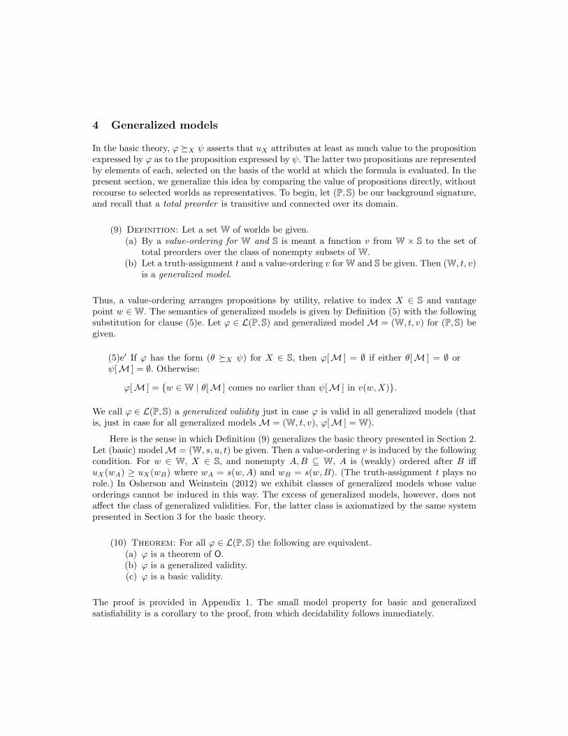
4 Generalized models

In the basic theory, ϕ X ψ asserts that uX attributes at least as much value to the propositionexpressed by ϕ as to the proposition expressed by ψ. The latter two propositions are representedby elements of each, selected on the basis of the world at which the formula is evaluated. In thepresent section, we generalize this idea by comparing the value of propositions directly, withoutrecourse to selected worlds as representatives. To begin, let (P,S) be our background signature,and recall that a total preorder is transitive and connected over its domain.

(9) Definition: Let a set W of worlds be given.(a) By a value-ordering for W and S is meant a function v from W × S to the set of

total preorders over the class of nonempty subsets of W.(b) Let a truth-assignment t and a value-ordering v for W and S be given. Then (W, t, v)

is a generalized model.

Thus, a value-ordering arranges propositions by utility, relative to index X ∈ S and vantagepoint w ∈W. The semantics of generalized models is given by Definition (5) with the followingsubstitution for clause (5)e. Let ϕ ∈ L(P,S) and generalized model M = (W, t, v) for (P,S) begiven.

(5)e′ If ϕ has the form (θ X ψ) for X ∈ S, then ϕ[M ] = ∅ if either θ[M ] = ∅ orψ[M ] = ∅. Otherwise:

ϕ[M ] = w ∈W | θ[M ] comes no earlier than ψ[M ] in v(w,X).

We call ϕ ∈ L(P,S) a generalized validity just in case ϕ is valid in all generalized models (thatis, just in case for all generalized models M = (W, t, v), ϕ[M ] = W).

Here is the sense in which Definition (9) generalizes the basic theory presented in Section 2.Let (basic) modelM = (W, s, u, t) be given. Then a value-ordering v is induced by the followingcondition. For w ∈ W, X ∈ S, and nonempty A,B ⊆ W, A is (weakly) ordered after B iffuX(wA) ≥ uX(wB) where wA = s(w,A) and wB = s(w,B). (The truth-assignment t plays norole.) In Osherson and Weinstein (2012) we exhibit classes of generalized models whose valueorderings cannot be induced in this way. The excess of generalized models, however, does notaffect the class of generalized validities. For, the latter class is axiomatized by the same systempresented in Section 3 for the basic theory.

(10) Theorem: For all ϕ ∈ L(P,S) the following are equivalent.(a) ϕ is a theorem of O.(b) ϕ is a generalized validity.(c) ϕ is a basic validity.

The proof is provided in Appendix 1. The small model property for basic and generalizedsatisfiability is a corollary to the proof, from which decidability follows immediately.

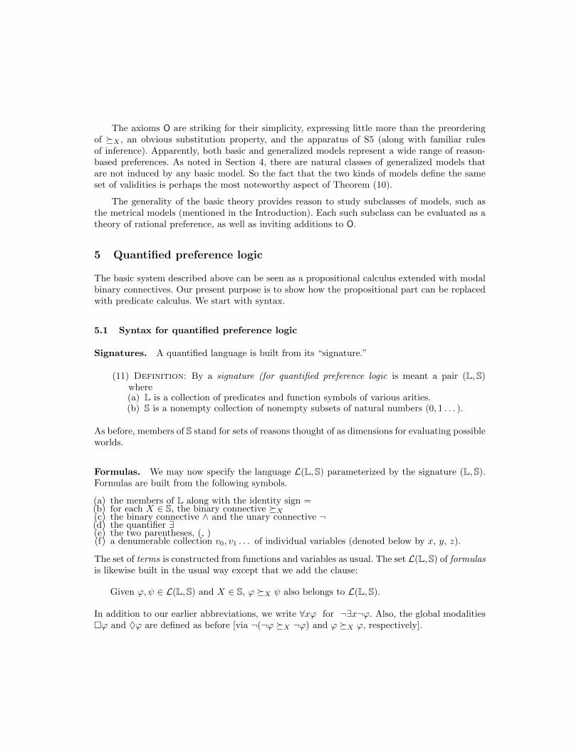
The axioms O are striking for their simplicity, expressing little more than the preorderingof X , an obvious substitution property, and the apparatus of S5 (along with familiar rulesof inference). Apparently, both basic and generalized models represent a wide range of reason-based preferences. As noted in Section 4, there are natural classes of generalized models thatare not induced by any basic model. So the fact that the two kinds of models define the sameset of validities is perhaps the most noteworthy aspect of Theorem (10).

The generality of the basic theory provides reason to study subclasses of models, such asthe metrical models (mentioned in the Introduction). Each such subclass can be evaluated as atheory of rational preference, as well as inviting additions to O.

5 Quantified preference logic

The basic system described above can be seen as a propositional calculus extended with modalbinary connectives. Our present purpose is to show how the propositional part can be replacedwith predicate calculus. We start with syntax.

5.1 Syntax for quantified preference logic

Signatures. A quantified language is built from its “signature.”

(11) Definition: By a signature (for quantified preference logic is meant a pair (L,S)where(a) L is a collection of predicates and function symbols of various arities.(b) S is a nonempty collection of nonempty subsets of natural numbers (0, 1 . . . ).

As before, members of S stand for sets of reasons thought of as dimensions for evaluating possibleworlds.

Formulas. We may now specify the language L(L,S) parameterized by the signature (L,S).Formulas are built from the following symbols.

(a) the members of L along with the identity sign =(b) for each X ∈ S, the binary connective X(c) the binary connective ∧ and the unary connective ¬(d) the quantifier ∃(e) the two parentheses, (, )(f) a denumerable collection v0, v1 . . . of individual variables (denoted below by x, y, z).

The set of terms is constructed from functions and variables as usual. The set L(L,S) of formulasis likewise built in the usual way except that we add the clause:

Given ϕ,ψ ∈ L(L,S) and X ∈ S, ϕ X ψ also belongs to L(L,S).

In addition to our earlier abbreviations, we write ∀xϕ for ¬∃x¬ϕ. Also, the global modalitiesϕ and ♦ϕ are defined as before [via ¬(¬ϕ X ¬ϕ) and ϕ X ϕ, respectively].

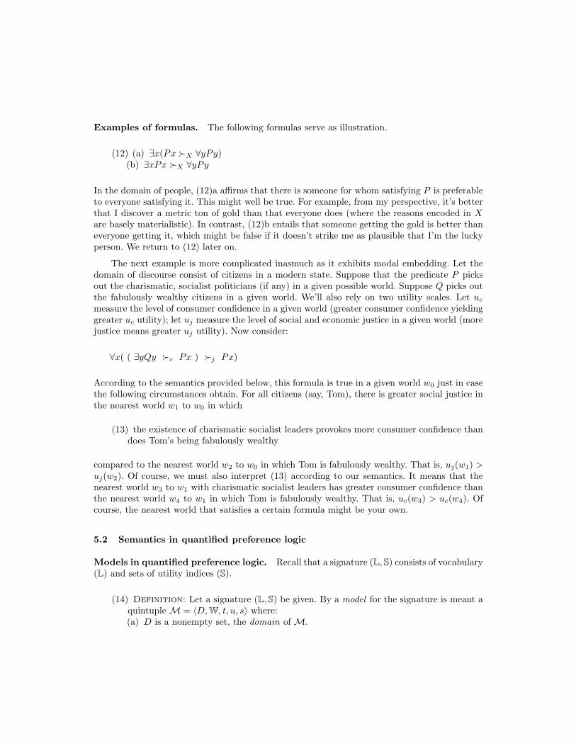
Examples of formulas. The following formulas serve as illustration.

(12) (a) ∃x(Px X ∀yPy)(b) ∃xPx X ∀yPy

In the domain of people, (12)a affirms that there is someone for whom satisfying P is preferableto everyone satisfying it. This might well be true. For example, from my perspective, it’s betterthat I discover a metric ton of gold than that everyone does (where the reasons encoded in Xare basely materialistic). In contrast, (12)b entails that someone getting the gold is better thaneveryone getting it, which might be false if it doesn’t strike me as plausible that I’m the luckyperson. We return to (12) later on.

The next example is more complicated inasmuch as it exhibits modal embedding. Let thedomain of discourse consist of citizens in a modern state. Suppose that the predicate P picksout the charismatic, socialist politicians (if any) in a given possible world. Suppose Q picks outthe fabulously wealthy citizens in a given world. We’ll also rely on two utility scales. Let ucmeasure the level of consumer confidence in a given world (greater consumer confidence yieldinggreater uc utility); let uj measure the level of social and economic justice in a given world (morejustice means greater uj utility). Now consider:

∀x( ( ∃yQy c Px ) j Px)

According to the semantics provided below, this formula is true in a given world w0 just in casethe following circumstances obtain. For all citizens (say, Tom), there is greater social justice inthe nearest world w1 to w0 in which

(13) the existence of charismatic socialist leaders provokes more consumer confidence thandoes Tom’s being fabulously wealthy

compared to the nearest world w2 to w0 in which Tom is fabulously wealthy. That is, uj(w1) >uj(w2). Of course, we must also interpret (13) according to our semantics. It means that thenearest world w3 to w1 with charismatic socialist leaders has greater consumer confidence thanthe nearest world w4 to w1 in which Tom is fabulously wealthy. That is, uc(w3) > uc(w4). Ofcourse, the nearest world that satisfies a certain formula might be your own.

5.2 Semantics in quantified preference logic

Models in quantified preference logic. Recall that a signature (L,S) consists of vocabulary(L) and sets of utility indices (S).

(14) Definition: Let a signature (L,S) be given. By a model for the signature is meant aquintuple M = 〈D,W, t, u, s〉 where:(a) D is a nonempty set, the domain of M.

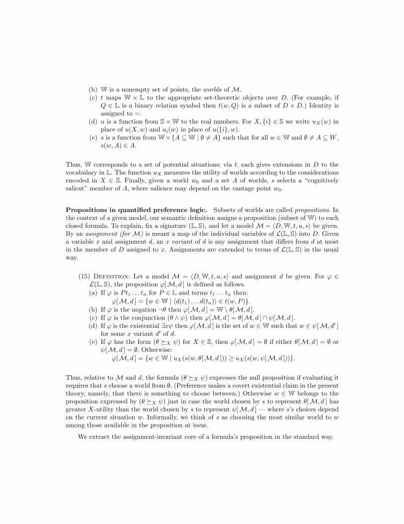
(b) W is a nonempty set of points, the worlds of M.(c) t maps W × L to the appropriate set-theoretic objects over D. (For example, if

Q ∈ L is a binary relation symbol then t(w,Q) is a subset of D × D.) Identity isassigned to =.

(d) u is a function from S×W to the real numbers. For X, i ∈ S we write uX(w) inplace of u(X,w) and ui(w) in place of u(i, w).

(e) s is a function from W×A ⊆W | ∅ 6= A such that for all w ∈W and ∅ 6= A ⊆W ,s(w,A) ∈ A.

Thus, W corresponds to a set of potential situations; via t, each gives extensions in D to thevocabulary in L. The function uX measures the utility of worlds according to the considerationsencoded in X ∈ S. Finally, given a world w0 and a set A of worlds, s selects a “cognitivelysalient” member of A, where salience may depend on the vantage point w0.

Propositions in quantified preference logic. Subsets of worlds are called propositions. Inthe context of a given model, our semantic definition assigns a proposition (subset of W) to eachclosed formula. To explain, fix a signature (L,S), and let a model M = 〈D,W, t, u, s〉 be given.By an assignment (for M) is meant a map of the individual variables of L(L,S) into D. Givena variable x and assignment d, an x variant of d is any assignment that differs from d at mostin the member of D assigned to x. Assignments are extended to terms of L(L,S) in the usualway.

(15) Definition: Let a model M = 〈D,W, t, u, s〉 and assignment d be given. For ϕ ∈L(L,S), the proposition ϕ[M, d ] is defined as follows.

(a) If ϕ is Pt1 . . . tn for P ∈ L and terms t1 . . . tn then:

ϕ[M, d ] = w ∈W | 〈d(t1) . . . d(tn)〉 ∈ t(w,P ).(b) If ϕ is the negation ¬θ then ϕ[M, d ] = W \ θ[M, d ].(c) If ϕ is the conjunction (θ ∧ ψ) then ϕ[M, d ] = θ[M, d ] ∩ ψ[M, d ].(d) If ϕ is the existential ∃xψ then ϕ[M, d ] is the set of w ∈W such that w ∈ ψ[M, d′ ]

for some x variant d′ of d.(e) If ϕ has the form (θ X ψ) for X ∈ S, then ϕ[M, d ] = ∅ if either θ[M, d ] = ∅ or

ψ[M, d ] = ∅. Otherwise:

ϕ[M, d ] = w ∈W | uX(s(w, θ[M, d ])) ≥ uX(s(w,ψ[M, d ])).

Thus, relative to M and d, the formula (θ X ψ) expresses the null proposition if evaluating itrequires that s choose a world from ∅. (Preference makes a covert existential claim in the presenttheory, namely, that there is something to choose between.) Otherwise w ∈ W belongs to theproposition expressed by (θ X ψ) just in case the world chosen by s to represent θ[M, d ] hasgreater X-utility than the world chosen by s to represent ψ[M, d ] — where s’s choices dependon the current situation w. Informally, we think of s as choosing the most similar world to wamong those available in the proposition at issue.

We extract the assignment-invariant core of a formula’s proposition in the standard way.

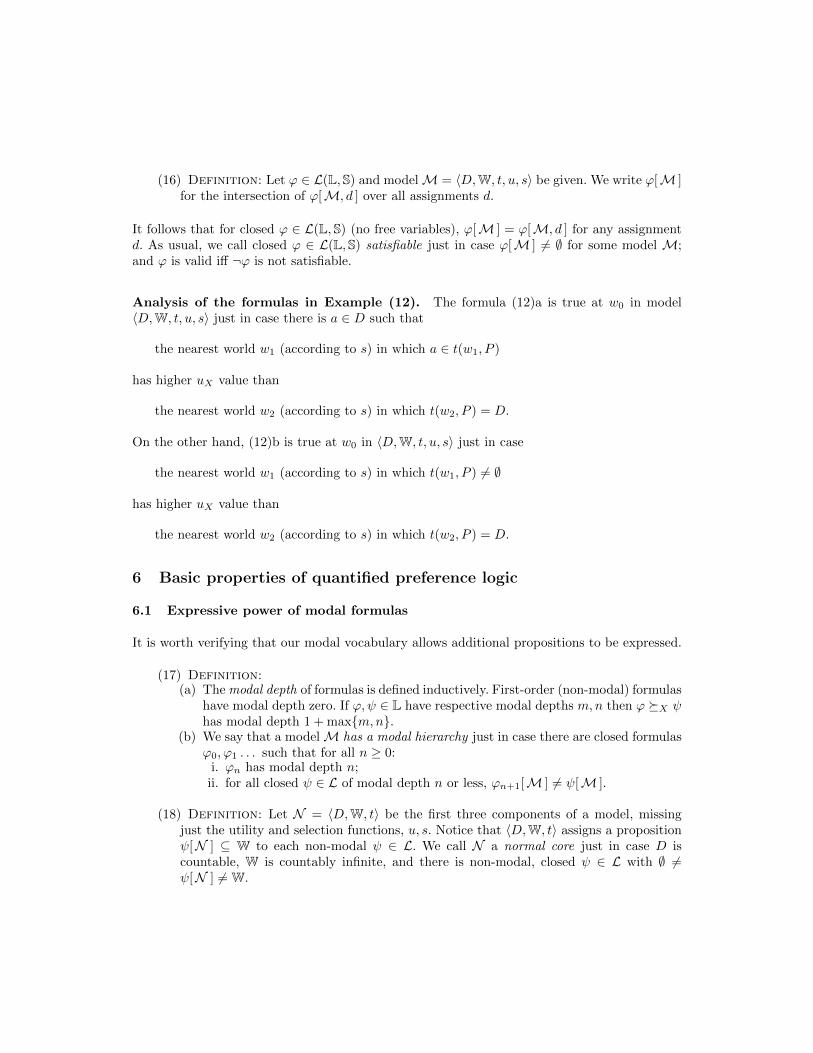
(16) Definition: Let ϕ ∈ L(L,S) and modelM = 〈D,W, t, u, s〉 be given. We write ϕ[M ]for the intersection of ϕ[M, d ] over all assignments d.

It follows that for closed ϕ ∈ L(L,S) (no free variables), ϕ[M ] = ϕ[M, d ] for any assignmentd. As usual, we call closed ϕ ∈ L(L,S) satisfiable just in case ϕ[M ] 6= ∅ for some model M;and ϕ is valid iff ¬ϕ is not satisfiable.

Analysis of the formulas in Example (12). The formula (12)a is true at w0 in model〈D,W, t, u, s〉 just in case there is a ∈ D such that

the nearest world w1 (according to s) in which a ∈ t(w1, P )

has higher uX value than

the nearest world w2 (according to s) in which t(w2, P ) = D.

On the other hand, (12)b is true at w0 in 〈D,W, t, u, s〉 just in case

the nearest world w1 (according to s) in which t(w1, P ) 6= ∅

has higher uX value than

the nearest world w2 (according to s) in which t(w2, P ) = D.

6 Basic properties of quantified preference logic

6.1 Expressive power of modal formulas

It is worth verifying that our modal vocabulary allows additional propositions to be expressed.

(17) Definition:(a) The modal depth of formulas is defined inductively. First-order (non-modal) formulas

have modal depth zero. If ϕ,ψ ∈ L have respective modal depths m,n then ϕ X ψhas modal depth 1 + maxm,n.

(b) We say that a modelM has a modal hierarchy just in case there are closed formulasϕ0, ϕ1 . . . such that for all n ≥ 0:

i. ϕn has modal depth n;ii. for all closed ψ ∈ L of modal depth n or less, ϕn+1[M ] 6= ψ[M ].

(18) Definition: Let N = 〈D,W, t〉 be the first three components of a model, missingjust the utility and selection functions, u, s. Notice that 〈D,W, t〉 assigns a propositionψ[N ] ⊆ W to each non-modal ψ ∈ L. We call N a normal core just in case D iscountable, W is countably infinite, and there is non-modal, closed ψ ∈ L with ∅ 6=ψ[N ] 6= W.

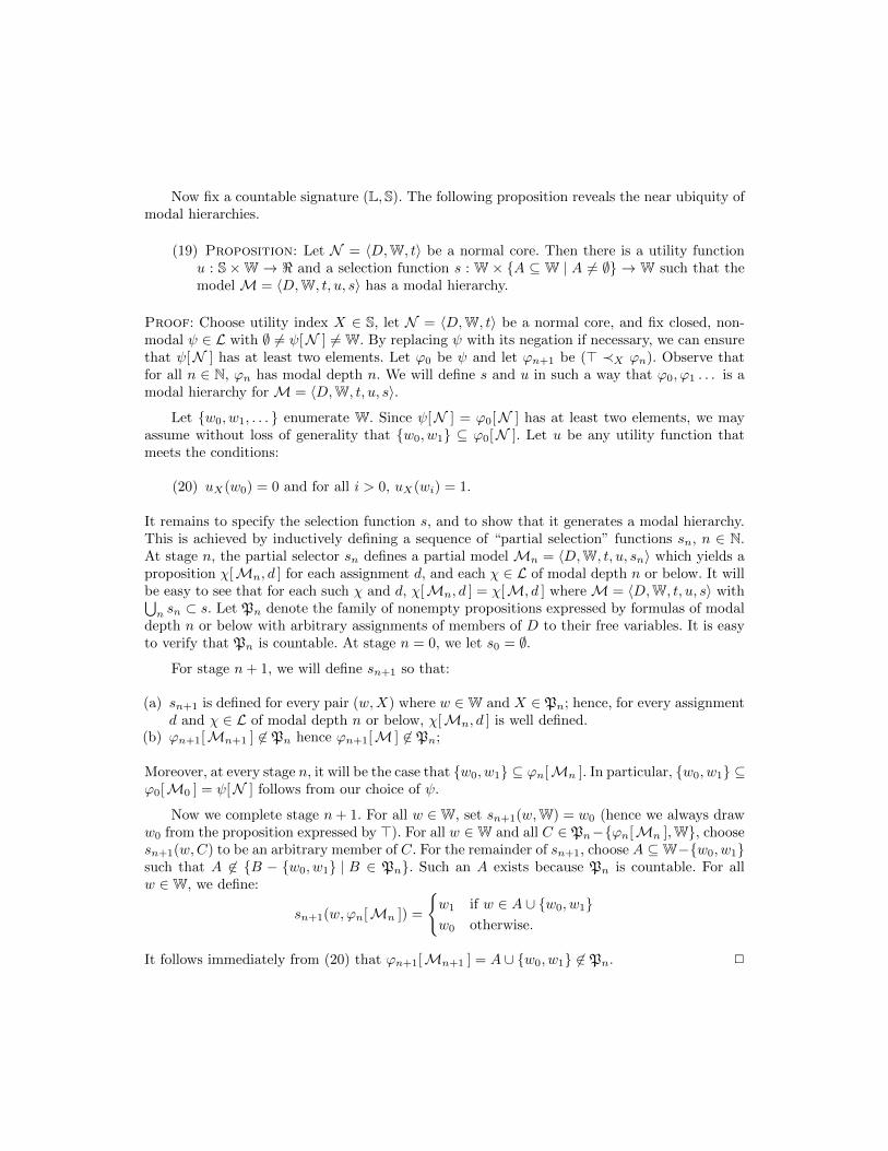
Now fix a countable signature (L,S). The following proposition reveals the near ubiquity ofmodal hierarchies.

(19) Proposition: Let N = 〈D,W, t〉 be a normal core. Then there is a utility functionu : S ×W → < and a selection function s : W × A ⊆ W | A 6= ∅ → W such that themodel M = 〈D,W, t, u, s〉 has a modal hierarchy.

Proof: Choose utility index X ∈ S, let N = 〈D,W, t〉 be a normal core, and fix closed, non-modal ψ ∈ L with ∅ 6= ψ[N ] 6= W. By replacing ψ with its negation if necessary, we can ensurethat ψ[N ] has at least two elements. Let ϕ0 be ψ and let ϕn+1 be (> ≺X ϕn). Observe thatfor all n ∈ N, ϕn has modal depth n. We will define s and u in such a way that ϕ0, ϕ1 . . . is amodal hierarchy for M = 〈D,W, t, u, s〉.

Let w0, w1, . . . enumerate W. Since ψ[N ] = ϕ0[N ] has at least two elements, we mayassume without loss of generality that w0, w1 ⊆ ϕ0[N ]. Let u be any utility function thatmeets the conditions:

(20) uX(w0) = 0 and for all i > 0, uX(wi) = 1.

It remains to specify the selection function s, and to show that it generates a modal hierarchy.This is achieved by inductively defining a sequence of “partial selection” functions sn, n ∈ N.At stage n, the partial selector sn defines a partial model Mn = 〈D,W, t, u, sn〉 which yields aproposition χ[Mn, d ] for each assignment d, and each χ ∈ L of modal depth n or below. It willbe easy to see that for each such χ and d, χ[Mn, d ] = χ[M, d ] whereM = 〈D,W, t, u, s〉 with⋃

n sn ⊂ s. Let Pn denote the family of nonempty propositions expressed by formulas of modaldepth n or below with arbitrary assignments of members of D to their free variables. It is easyto verify that Pn is countable. At stage n = 0, we let s0 = ∅.

For stage n+ 1, we will define sn+1 so that:

(a) sn+1 is defined for every pair (w,X) where w ∈W and X ∈ Pn; hence, for every assignmentd and χ ∈ L of modal depth n or below, χ[Mn, d ] is well defined.

(b) ϕn+1[Mn+1 ] 6∈ Pn hence ϕn+1[M ] 6∈ Pn;

Moreover, at every stage n, it will be the case that w0, w1 ⊆ ϕn[Mn ]. In particular, w0, w1 ⊆ϕ0[M0 ] = ψ[N ] follows from our choice of ψ.

Now we complete stage n+ 1. For all w ∈W, set sn+1(w,W) = w0 (hence we always draww0 from the proposition expressed by >). For all w ∈W and all C ∈ Pn−ϕn[Mn ],W, choosesn+1(w,C) to be an arbitrary member of C. For the remainder of sn+1, choose A ⊆W−w0, w1such that A 6∈ B − w0, w1 | B ∈ Pn. Such an A exists because Pn is countable. For allw ∈W, we define:

sn+1(w,ϕn[Mn ]) =

w1 if w ∈ A ∪ w0, w1w0 otherwise.

It follows immediately from (20) that ϕn+1[Mn+1 ] = A ∪ w0, w1 6∈ Pn. 2

A natural question about Proposition (19) is whether modal hierarchies still appear whenmodels satisfy various frame properties. To illustrate, model M = 〈D,W, t, u, s〉 is called “re-flexive” just in case for all w ∈W and A ⊆W, if w ∈ A then s(w,A) = w. Reflexivity embodiesthe idea that the actual world is closer to home than any other world. Several frame propertiesare examined in Osherson and Weinstein (2012), and also below. In the case of reflexivity, theforegoing proof can be adjusted to show that any normal core can be extended to a reflexivemodel with modal hierarchy. We leave unexplored the larger project of characterizing the frameproperties that allow modal hierarchies, or identifying natural properties that do not.

6.2 Undecidability of satisfaction

Suppose that the signature (L,S) contains two unary predicates P,Q ∈ L. Then it follows fromthe argument in Kripke (1962) that:

(21) Proposition: The satisfiable subset of L(L,S) is not decidable.

Kripke’s argument hinges on a mapping from first-order sentences with just the binary relationsymbol R to modal sentences that replace Rxy with ♦(Px ∧ Qy). On the other hand, thevalidities are axiomatizable:

(22) Proposition: If the signature is effectively enumerable then so is the set of validformulas in quantified preference logic.

This fact follows from Proposition (27), below.

6.3 Size of models

Suppose that the signature contains a binary predicate G. Then the upward Lowenheim-Skolemproperty fails to apply to quantified preference logic. Indeed:

(23) Proposition: There is ϕ ∈ L(L,S) such that:(a) Some model 〈D,W, t, u, s〉 with D countable satisfies ϕ.(b) No model 〈D,W, t, u, s〉 with D uncountable satisfies ϕ.

Proof: Basically, ϕ says that ≺ is a lexicographical order on D ×D; such an order cannot beembedded in 〈<, <〉 if D is uncountable. For typographical simplicity, we choose X ∈ S, andwrite ≺ in place of ≺X .

Specifically, we take ϕ to be the conjunction of the following formulas.

(24) (a) ∀x∀y(x 6= y → ((Gxx ≺ Gyy) ∨ (Gyy ≺ Gxx))(b) ∀x1y1x2y2((Gx1y1 ≺ Gx2y2) ↔ ((Gx1x1 ≺ Gx2x2) ∨ ((x1 = x2) ∧ (Gy1y1 ≺

Gy2y2))))

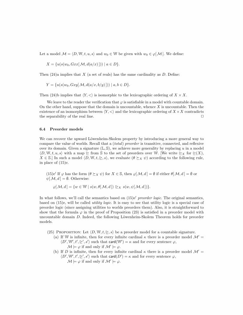
Let a model M = 〈D,W, t, u, s〉 and w0 ∈W be given with w0 ∈ ϕ[M ]. We define:

X = u(s(w0, Gxx[M, d(a/x) ])) | a ∈ D.

Then (24)a implies that X (a set of reals) has the same cardinality as D. Define:

Y = u(s(w0, Gxy[M, d(a/x, b/y) ])) | a, b ∈ D.

Then (24)b implies that 〈Y,<〉 is isomorphic to the lexicographic ordering of X ×X.

We leave to the reader the verification that ϕ is satisfiable in a model with countable domain.On the other hand, suppose that the domain is uncountable, whence X is uncountable. Then theexistence of an isomorphism between 〈Y,<〉 and the lexicographic ordering of X×X contradictsthe separability of the real line. 2

6.4 Preorder models

We can recover the upward Lowenheim-Skolem property by introducing a more general way tocompare the value of worlds. Recall that a (total) preorder is transitive, connected, and reflexiveover its domain. Given a signature (L,S), we achieve more generality by replacing u in a model〈D,W, t, u, s〉 with a map from S to the set of preorders over W. [We write X for (X),X ∈ S.] In such a model 〈D,W, t,, s〉, we evaluate (θ X ψ) according to the following rule,in place of (15)e.

(15)e′ If ϕ has the form (θ X ψ) for X ∈ S, then ϕ[M, d ] = ∅ if either θ[M, d ] = ∅ orψ[M, d ] = ∅. Otherwise:

ϕ[M, d ] = w ∈W | s(w, θ[M, d ]) X s(w,ψ[M, d ]).

In what follows, we’ll call the semantics based on (15)e′ preorder logic. The original semantics,based on (15)e, will be called utility logic. It is easy to see that utility logic is a special case ofpreorder logic (since assigning utilities to worlds preorders them). Also, it is straightforward toshow that the formula ϕ in the proof of Proposition (23) is satisfied in a preorder model withuncountable domain D. Indeed, the following Lowenheim-Skolem Theorem holds for preordermodels.

(25) Proposition: Let 〈D,W, t,, s〉 be a preorder model for a countable signature.(a) If W is infinite, then for every infinite cardinal κ there is a preorder model M′ =〈D′,W′, t′,′, s′〉 such that card(W′) = κ and for every sentence ϕ,M |= ϕ if and only if M′ |= ϕ.

(b) If D is infinite, then for every infinite cardinal κ there is a preorder model M′ =〈D′,W′, t′,′, s′〉 such that card(D′) = κ and for every sentence ϕ,M |= ϕ if and only if M′ |= ϕ.

Despite the greater generality of preorder logic, and the contrast between Propositions (25)and (23), the distinction between utility and preorder models is not discernible by formulas.Indeed:

(26) Proposition: A formula θ is valid in the class of utility models if and only if it isvalid in the class of preorder models.

Finally, the next proposition shows that the set of formulas which are valid in preorder models(and hence utility models, by the preceding proposition) is axiomatizable. We assume that thesignature is effectively enumerable.

(27) Proposition: The set of formulas which are valid in preorder models is effectivelyenumerable.

Proofs of Propositions (25), (26), and (27) are given in the Appendix 2. We have not investigatedthe quantified version of “generalized logic,” introduced in Section 4 above.

7 Subclasses of utility models

For the remainder of the discussion, only utility models (introduced in Section 5.2) are at issue.(We leave preorder models to one side.)

7.1 Metricity

Many interesting properties of a model 〈D,W, t, u, s〉 can formulated just in terms of W and s(the model’s “frame”). For example, Osherson and Weinstein (2012) consider the following wayto express the idea that s chooses “the nearest world.”

(28) Definition: A model 〈D,W, t, u, s〉 is metric just in case there is a metric d : W×W→< such that for all w ∈ W and ∅ 6= A ⊆ W, s(w,A) is the unique d-closest member ofA to w.

Note that a model is metric only if d-closest worlds exist (there are no chains of worlds everd-closer to a given world). It is easy to see that in a metric model the set of worlds is countable.There are several properties of models that are implied by metricity, including the followingtwo, articulated by Stalnaker (1968).

(29) Definition: Let model M = 〈D,W, t, u, s〉 be given.

(a) M is reflexive just in case for all A ⊆W and w ∈ A, s(w,A) = w.(b) M is regular just in case for all A ⊆ B ⊆ W and w ∈ W, s(w,B) ∈ A implies

s(w,A) = s(w,B).

These properties are explored in Osherson and Weinstein (2012). Here we focus on:

(30) Definition: A model 〈D,W, t, u, s〉 is transitive just in case for all A,B,C ⊆W withA,B 6= ∅, and w0 ∈W, if s(w0, A ∪B) ∈ A and s(w0, B ∪ C) ∈ B then s(w0, A ∪ C) =s(w0, A ∪B).

Exploiting our quantificational apparatus, we can write a formula that is true in all transitivemodels but not valid. We assume that the signature includes the predicate P . For notationalease, we suppress the X on ≈X .

(31) Proposition: Let ϕ be the conjunction of the following formulas.

(a) ∀xy(x 6= y → (Px 6≈ Py))

(b) ∀xyz ((x 6= y ∧ y 6= z ∧ x 6= z) → ((((Px ∨ Py) ≈ Px) ∧ ((Py ∨ Pz) ≈ Py)) →(Px ∨ Pz) ≈ Px))

Then ϕ is invalid but valid in the class of transitive models.

The proposition can be viewed as expressing the transitivity of revealed preference, e.g., (Px ∨Py) ≈ Px says that Px is chosen from the mutually exclusive options Px, Py.

Proof: Let modelM = 〈D,W, t, u, s〉, w0 ∈W and assignment d be given. Let Px[M, d ] =A, Py[M, d ] = B and Pz[M, d ] = C. If any of d(x), d(y), d(z) are identical or either A orB are empty then we are done. Otherwise, in the presence of (31)a, (Px ∨ Py) ≈ Px and(Py∨Pz) ≈ Py imply respectively that s(w0, A∪B) ∈ A and s(w0, B ∪C) ∈ B. So transitivityimplies s(w0, A ∪ C) = s(w0, A ∪B) which entails w0 ∈ (Px ∨ Pz) ≈ (Px ∨ Py)[M, d ]. So theproposition follows by the transitivity of ≈ from w0 ∈ (Px ∨ Py) ≈ Px[M, d ]. 2

7.2 Beyond the frame

Rational agents might not be able to discriminate between isomorphic worlds. To formulate thisidea, fix a signature (L,S), and let model M = 〈D,W, t, u, s〉 be given. We say that v, w ∈ Ware isomorphic (v ' w) just in case there is a permutation h of D such that for all Q ∈ L, h(applied component-wise) maps t(v,Q) onto t(w,Q).

(32) Definition: Model 〈D,W, t, u, s〉 is utility-invariant just in case for all isomorphicv, w ∈W, uX(v) = uX(w) for all X ∈ S.

This is not a frame property because all components of the model are involved in its formulation.Validity in the utility-invariant models doesn’t imply validity in the strict sense. Indeed, we have:

(33) Proposition: Let signature (L,S) be given with L finite, and distinct X,Y ∈ S. Thenthere is invalid ϕ ∈ L(L,S) that is valid in the class of utility-invariant models.

Proof: There is χ ∈ L(L,S) such that for all models M = 〈D,W, t, u, s〉, χ[M ] = W iff| D | = 2. Hence, by the finitude of L and the presence of identity, there is closed, satisfiableψ ∈ L(L,S) such that for all models M, if w1, w2 ∈ ψ[M ] then w1 ' w2. Let the promised ϕbe:

(ψ ∧ (ψ X >) ∧ (ψ Y >))→ ((ψ ∧ (ψ X >)) ≈X (ψ ∧ (ψ Y >))).

We indicate why ϕ is invalid. The antecedent of ϕ is easily seen to be satisfiable, and a ψ-worldsatisfying ψ ∧ (ψ X >) need not be the same world that satisfies ψ ∧ (ψ Y >)); and uX maybe chosen to be injective.

On the other hand, suppose that model M = 〈D,W, t, u, s〉 is utility-invariant and letw0 ∈ W. Suppose that the antecedent of ϕ is satisfiable in M (otherwise, we are done). Then(ψ ∧ (ψ X >)[M ] 6= ∅ and (ψ ∧ (ψ Y >))[M ] 6= ∅. So, let w1 = s(w0, (ψ ∧ (ψ X >))[M ])and w2 = s(w0, ψ ∧ (ψ Y >)))[M ]). Then each of w1, w2 satisfies ψ so w1 ' w2. HenceuX(w1) = uX(w2) by utility-invariance. 2

8 Anonymity

Our next topic concerns the manner in which utilities are associated with formulas. First, acondition is exhibited that makes the utility of a conjunction depend on just the utilities of eachconjunct separately. According to this condition the vocabulary appearing in a conjunct is notpermitted to influence the utility of the conjunction; rather, the conjunct contributes its utility“anonymously.” A second condition is then introduced that entails a similar kind of anonymityfor the contribution of utility indexes 1 and 2 to the aggregated utility 1, 2. The material inthis section is inspired by the discussion in Krantz et al. (1971, §7.2).

8.1 Decomposing the utility of conjunctions

Let a signature (L,S) be given with predicate P ∈ L. Conjunctive anonymity with respect to Pis expressed by the following formula. (To lighten notation, we suppress X ∈ S in subscripts.)

(34) ϕdef= ∀xy((Px ≈ Py)→ ∀z((Px ∧ Pz) ≈ (Py ∧ Pz)))

The next proposition gives the sense in which ϕ causes the utility of Px ∧ Py to be a function(F ) of the utilities of Px and Py.

(35) Proposition: Let model M = 〈D,W, t, u, s〉 be given with w0 ∈ ϕ[M ]. Then thereis a function F : <2 → < such that for all assignments d with Px ∧ Py[M, d ] 6= ∅,

u(s(w0, Px ∧ Py[M, d ])) = F (u(s(w0, Px[M, d ])), u(s(w0, Py[M, d ])) ).

Proof: For numbers of the form u(s(w0, Px[M, d ])) and u(s(w0, Py[M, d ])) define:

(36) F (u(s(w0, Px[M, d ])), u(s(w0, Py[M, d ])) )def= u(s(w0, Px ∧ Py[M, d ])).

For all other numbers r1, r2, F (r1, r2) is defined arbitrarily. We must show that F is a function.For this purpose, let variable q be given, and suppose that

(37) u(s(w0, Px[M, d ])) = u(s(w0, P q[M, d ])).

To finish the proof it suffices to show that

(38) u(s(w0, Px ∧ Py[M, d ])) = u(s(w0, P q ∧ Py[M, d ])),

the second argument of F being treated in the same way. It follows immediately from (37) thatw0 ∈ (Px ≈ Pq)[M, d ], hence by (34)

w0 ∈ ((Px ∧ Py) ≈ (Pq ∧ Py))[M, d ],

which implies (38). 2

Observe that ϕ and Proposition (35) can be formulated with disjunction in place of con-junction — or with many other formulas. The proof proceeds in the same way.

8.2 Decomposing a complex utility index

Suppose for this section that the signature (L,S) contains unary P ∈ L along with 1, 2, 1, 2 ∈S. Define:

(39) ϕdef= ∀xy( ((Px ≈1 Py) ∧ (Px ≈2 Py))→ (Px ≈1,2 Py) ).

Then ϕ implies that the contributions of 1 and 2 to the complex utility index 1, 2 can beseparated then brought back together via a binary mapping on <. Specifically:

(40) Proposition: Let model M = 〈D,W, t, u, s〉 be given with w0 ∈ ϕ[M ]. Then thereis a function F : <2 → < such that for all assignments d:

u1,2(s(w0, Px[M, d ])) = F (u1(s(w0, Px[M, d ])), u2(s(w0, Px[M, d ])) ).

Proof: Call a pair (p, q) ∈ <2 critical just in case there is an assignment d such that

(41) (a) p = u1(s(w0, Px[M, d ]))(b) q = u2(s(w0, Px[M, d ])).

Let F : <2 → < be such that for any critical pair (p, q) as in(41), F (p, q) = u1,2(s(w0, Px[M, d ])).The behavior of F on noncritical pairs is arbitrary. Suppose that for some assignment d′:

(42) (a) p = u1(s(w0, Px[M, d′ ]))

(b) q = u2(s(w0, Px[M, d′ ])).

To verify that F is a function, thereby completing the proof, we must show that

(43) u1,2(s(w0, Px[M, d ])) = u1,2(s(w0, Px[M, d′ ])).

Let y be a variable distinct from x, and let d′′ = d(d′(x)/y). From (41) and (42) we infer:w0 ∈ Px ≈1 Py[M, d′′ ] and w0 ∈ Px ≈2 Py[M, d′′ ]. From (39) we then obtain w0 ∈ Px ≈1,2

Py[M, d′′ ] from which (43) is an immediate consequence. 2

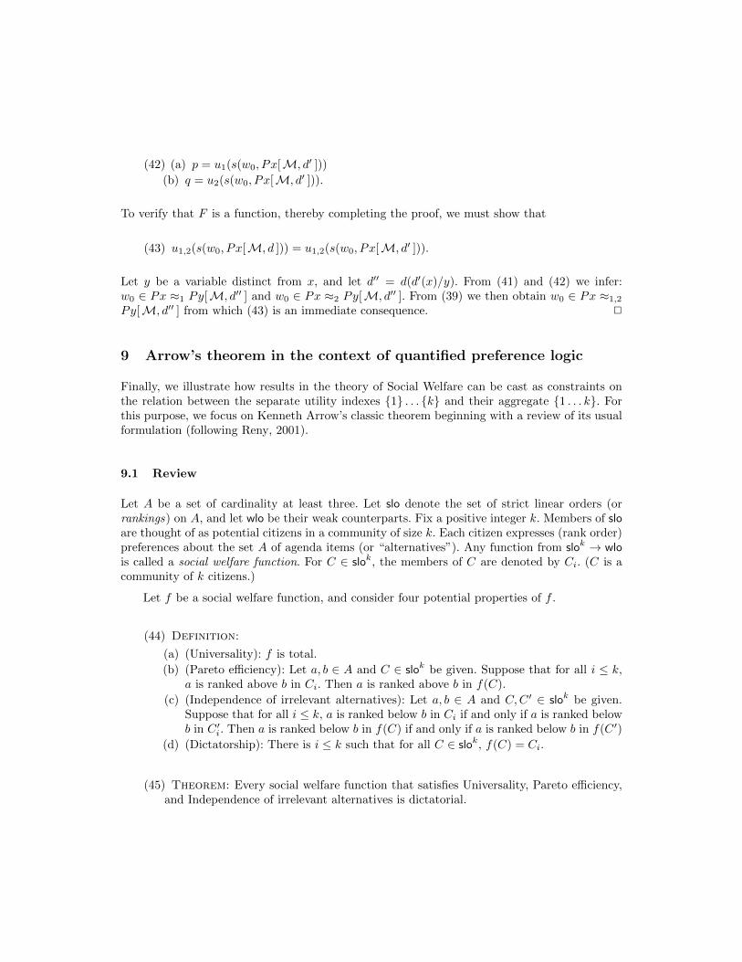
9 Arrow’s theorem in the context of quantified preference logic

Finally, we illustrate how results in the theory of Social Welfare can be cast as constraints onthe relation between the separate utility indexes 1 . . . k and their aggregate 1 . . . k. Forthis purpose, we focus on Kenneth Arrow’s classic theorem beginning with a review of its usualformulation (following Reny, 2001).

9.1 Review

Let A be a set of cardinality at least three. Let slo denote the set of strict linear orders (orrankings) on A, and let wlo be their weak counterparts. Fix a positive integer k. Members of sloare thought of as potential citizens in a community of size k. Each citizen expresses (rank order)preferences about the set A of agenda items (or “alternatives”). Any function from slok → wlois called a social welfare function. For C ∈ slok, the members of C are denoted by Ci. (C is acommunity of k citizens.)

Let f be a social welfare function, and consider four potential properties of f .

(44) Definition:

(a) (Universality): f is total.

(b) (Pareto efficiency): Let a, b ∈ A and C ∈ slok be given. Suppose that for all i ≤ k,a is ranked above b in Ci. Then a is ranked above b in f(C).

(c) (Independence of irrelevant alternatives): Let a, b ∈ A and C,C ′ ∈ slok be given.Suppose that for all i ≤ k, a is ranked below b in Ci if and only if a is ranked belowb in C ′i. Then a is ranked below b in f(C) if and only if a is ranked below b in f(C ′)

(d) (Dictatorship): There is i ≤ k such that for all C ∈ slok, f(C) = Ci.

(45) Theorem: Every social welfare function that satisfies Universality, Pareto efficiency,and Independence of irrelevant alternatives is dictatorial.

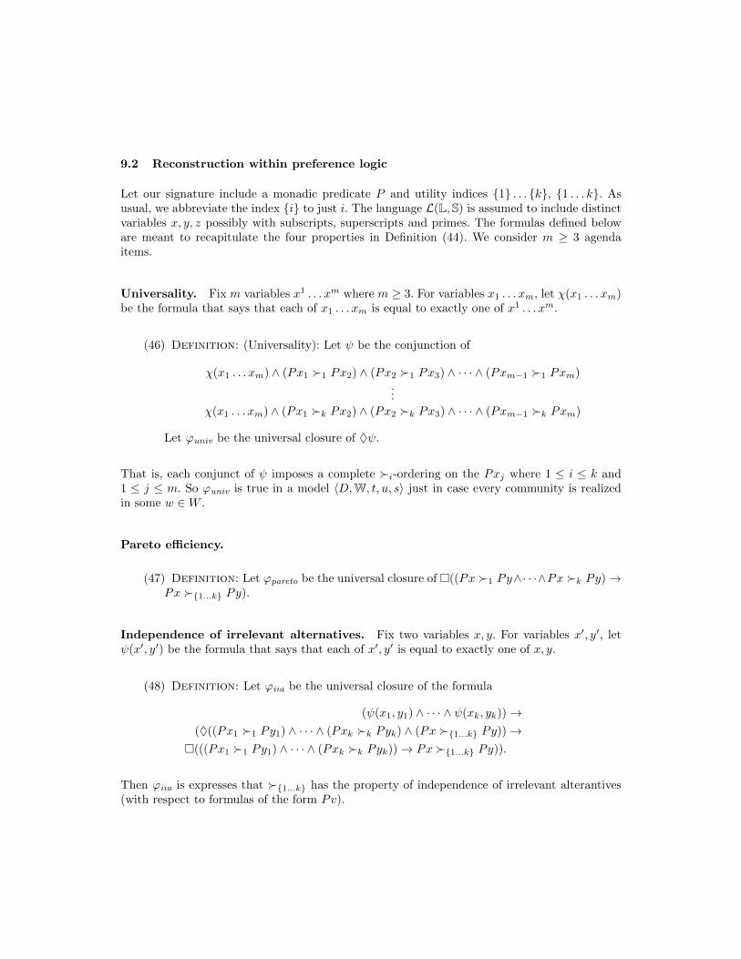
9.2 Reconstruction within preference logic

Let our signature include a monadic predicate P and utility indices 1 . . . k, 1 . . . k. Asusual, we abbreviate the index i to just i. The language L(L,S) is assumed to include distinctvariables x, y, z possibly with subscripts, superscripts and primes. The formulas defined beloware meant to recapitulate the four properties in Definition (44). We consider m ≥ 3 agendaitems.

Universality. Fix m variables x1 . . . xm where m ≥ 3. For variables x1 . . . xm, let χ(x1 . . . xm)be the formula that says that each of x1 . . . xm is equal to exactly one of x1 . . . xm.

(46) Definition: (Universality): Let ψ be the conjunction of

χ(x1 . . . xm) ∧ (Px1 1 Px2) ∧ (Px2 1 Px3) ∧ · · · ∧ (Pxm−1 1 Pxm)...

χ(x1 . . . xm) ∧ (Px1 k Px2) ∧ (Px2 k Px3) ∧ · · · ∧ (Pxm−1 k Pxm)

Let ϕuniv be the universal closure of ♦ψ.

That is, each conjunct of ψ imposes a complete i-ordering on the Pxj where 1 ≤ i ≤ k and1 ≤ j ≤ m. So ϕuniv is true in a model 〈D,W, t, u, s〉 just in case every community is realizedin some w ∈W .

Pareto efficiency.

(47) Definition: Let ϕpareto be the universal closure of ((Px 1 Py∧· · ·∧Px k Py)→Px 1...k Py).

Independence of irrelevant alternatives. Fix two variables x, y. For variables x′, y′, letψ(x′, y′) be the formula that says that each of x′, y′ is equal to exactly one of x, y.

(48) Definition: Let ϕiia be the universal closure of the formula

(ψ(x1, y1) ∧ · · · ∧ ψ(xk, yk))→(♦((Px1 1 Py1) ∧ · · · ∧ (Pxk k Pyk) ∧ (Px 1...k Py))→

(((Px1 1 Py1) ∧ · · · ∧ (Pxk k Pyk))→ Px 1...k Py)).

Then ϕiia is expresses that 1...k has the property of independence of irrelevant alterantives(with respect to formulas of the form Pv).

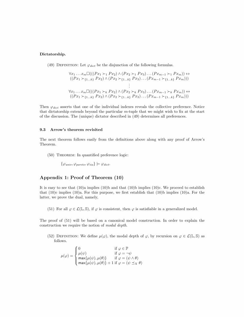
Dictatorship.

(49) Definition: Let ϕdict be the disjunction of the following formulas.

∀x1 . . . xm(((Px1 1 Px2) ∧ (Px2 1 Px3) . . . (Pxm−1 1 Pxm))↔((Px1 1...k Px2) ∧ (Px2 1...k Px3) . . . (Pxm−1 1...k Pxm)))

...∀x1 . . . xm(((Px1 k Px2) ∧ (Px2 k Px3) . . . (Pxm−1 k Pxm))↔((Px1 1...k Px2) ∧ (Px2 1...k Px3) . . . (Pxm−1 1...k Pxm)))

Then ϕdict asserts that one of the individual indexes reveals the collective preference. Noticethat dictatorship extends beyond the particular m-tuple that we might wish to fix at the startof the discussion. The (unique) dictator described in (49) determines all preferences.

9.3 Arrow’s theorem revisited

The next theorem follows easily from the definitions above along with any proof of Arrow’sTheorem.

(50) Theorem: In quantified preference logic:

ϕuniv, ϕpareto, ϕiia |= ϕdict.

Appendix 1: Proof of Theorem (10)

It is easy to see that (10)a implies (10)b and that (10)b implies (10)c. We proceed to establishthat (10)c implies (10)a. For this purpose, we first establish that (10)b implies (10)a. For thelatter, we prove the dual, namely,

(51) For all ϕ ∈ L(L,S), if ϕ is consistent, then ϕ is satisfiable in a generalized model.

The proof of (51) will be based on a canonical model construction. In order to explain theconstruction we require the notion of modal depth.

(52) Definition: We define µ(ϕ), the modal depth of ϕ, by recursion on ϕ ∈ L(L,S) asfollows.

µ(ϕ) =

0 if ϕ ∈ Pµ(ψ) if ϕ = ¬ψmaxµ(ψ), µ(θ) if ϕ = (ψ ∧ θ)maxµ(ψ), µ(θ)+ 1 if ϕ = (ψ X θ)

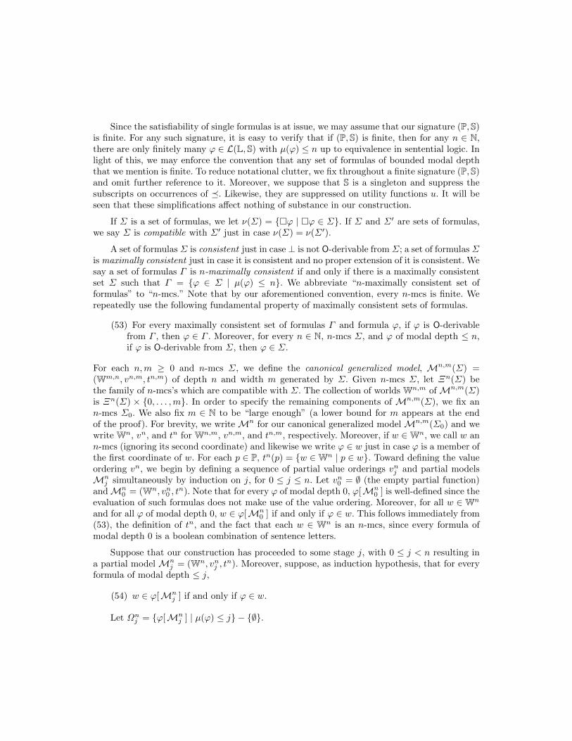
Since the satisfiability of single formulas is at issue, we may assume that our signature (P,S)is finite. For any such signature, it is easy to verify that if (P,S) is finite, then for any n ∈ N,there are only finitely many ϕ ∈ L(L,S) with µ(ϕ) ≤ n up to equivalence in sentential logic. Inlight of this, we may enforce the convention that any set of formulas of bounded modal depththat we mention is finite. To reduce notational clutter, we fix throughout a finite signature (P,S)and omit further reference to it. Moreover, we suppose that S is a singleton and suppress thesubscripts on occurrences of . Likewise, they are suppressed on utility functions u. It will beseen that these simplifications affect nothing of substance in our construction.

If Σ is a set of formulas, we let ν(Σ) = ϕ | ϕ ∈ Σ. If Σ and Σ′ are sets of formulas,we say Σ is compatible with Σ′ just in case ν(Σ) = ν(Σ′).

A set of formulas Σ is consistent just in case ⊥ is not O-derivable from Σ; a set of formulas Σis maximally consistent just in case it is consistent and no proper extension of it is consistent. Wesay a set of formulas Γ is n-maximally consistent if and only if there is a maximally consistentset Σ such that Γ = ϕ ∈ Σ | µ(ϕ) ≤ n. We abbreviate “n-maximally consistent set offormulas” to “n-mcs.” Note that by our aforementioned convention, every n-mcs is finite. Werepeatedly use the following fundamental property of maximally consistent sets of formulas.

(53) For every maximally consistent set of formulas Γ and formula ϕ, if ϕ is O-derivablefrom Γ , then ϕ ∈ Γ . Moreover, for every n ∈ N, n-mcs Σ, and ϕ of modal depth ≤ n,if ϕ is O-derivable from Σ, then ϕ ∈ Σ.

For each n,m ≥ 0 and n-mcs Σ, we define the canonical generalized model, Mn,m(Σ) =(Wm,n, vn,m, tn,m) of depth n and width m generated by Σ. Given n-mcs Σ, let Ξn(Σ) bethe family of n-mcs’s which are compatible with Σ. The collection of worlds Wn,m ofMn,m(Σ)is Ξn(Σ) × 0, . . . ,m. In order to specify the remaining components of Mn,m(Σ), we fix ann-mcs Σ0. We also fix m ∈ N to be “large enough” (a lower bound for m appears at the endof the proof). For brevity, we writeMn for our canonical generalized modelMn,m(Σ0) and wewrite Wn, vn, and tn for Wn,m, vn,m, and tn,m, respectively. Moreover, if w ∈Wn, we call w ann-mcs (ignoring its second coordinate) and likewise we write ϕ ∈ w just in case ϕ is a member ofthe first coordinate of w. For each p ∈ P, tn(p) = w ∈Wn | p ∈ w. Toward defining the valueordering vn, we begin by defining a sequence of partial value orderings vnj and partial modelsMn

j simultaneously by induction on j, for 0 ≤ j ≤ n. Let vn0 = ∅ (the empty partial function)andMn

0 = (Wn, vn0 , tn). Note that for every ϕ of modal depth 0, ϕ[Mn

0 ] is well-defined since theevaluation of such formulas does not make use of the value ordering. Moreover, for all w ∈Wn

and for all ϕ of modal depth 0, w ∈ ϕ[Mn0 ] if and only if ϕ ∈ w. This follows immediately from

(53), the definition of tn, and the fact that each w ∈ Wn is an n-mcs, since every formula ofmodal depth 0 is a boolean combination of sentence letters.

Suppose that our construction has proceeded to some stage j, with 0 ≤ j < n resulting ina partial model Mn

j = (Wn, vnj , tn). Moreover, suppose, as induction hypothesis, that for every

formula of modal depth ≤ j,

(54) w ∈ ϕ[Mnj ] if and only if ϕ ∈ w.

Let Ωnj = ϕ[Mn

j ] | µ(ϕ) ≤ j − ∅.

We proceed to specify vnj+1. For each w ∈ Wn, vnj+1(w) is the relation on Ωnj defined as

follows.

(55) For all ϕ and ψ with µ(ϕ), µ(ψ) ≤ j and ϕ[Mnj ], ψ[Mn

j ] non-empty,

〈ϕ[Mnj ], ψ[Mn

j ]〉 ∈ vnj+1(w) if and only if (ϕ ψ) ∈ w.

To complete the construction, we must verify that

(56) for all w ∈Wn and all formulas ϕ of modal depth ≤ j + 1,

(a) vnj+1(w) is a pre-order of Ωnj , and

(b) w ∈ ϕ[Mnj+1 ] if and only if ϕ ∈ w.

In order to establish (56)a, we argue as follows. Fix w ∈ Wn. We first show that vnj+1(w) iswell-defined, that is, if ϕ, ψ, and θ are formulas of modal depth ≤ j and ϕ[Mn

j ] = ψ[Mnj ],

then

(57) 〈ϕ[Mnj ], θ[Mn

j ]〉 ∈ vnj+1(w) if and only if 〈ψ[Mnj ], θ[Mn

j ]〉 ∈ vnj+1(w),

and similarly with ϕ and θ and ψ and θ reversed. So suppose that

(58) ϕ and ψ are formulas of modal depth ≤ j and ϕ[Mnj ] = ψ[Mn

j ].

It follows at once from (58), (54), and (53), recalling the fact that every w′ ∈Wn is an n-mcs,that

(59) for all w′ ∈Wn, (ϕ↔ ψ) ∈ w′.

Let χ be the conjunction of the formulas in ν(w). It follows from (59) and the definition of Wn

that

(60) χ→ (ϕ↔ ψ) is a theorem of O,

for otherwise, there would be an n-mcs w′ ∈Wn with ¬(ϕ↔ ψ) ∈ w′ contradicting (59). Sincethe theorems of O are closed under necessitation, (60) implies that

(61) (χ→ (ϕ↔ ψ)) is a theorem of O.

Moreover, since each w′ ∈ Wn is an n-mcs, θ → θ is a theorem of S5, and each of theconjuncts of χ is a “boxed” formula, it follows from (53) that

(62) for all w′ ∈Wn, and all maximally consistent sets of formulas Γ ⊃ w′, χ ∈ Γ .

It follows from (61), (62), and (53), and the S5 modal principle

(χ ∧(χ→ (ϕ↔ ψ)))→ (ϕ↔ ψ),

that

(63) (ϕ↔ ψ) ∈ w.

But then, by (53), (63), Axiom (8)c and the fact that w is an n-mcs,

(64) (ϕ θ) ∈ w if and only if (ψ θ) ∈ w.

Therefore vnj+1 is well-defined, since (57) follows directly from (64) and (55).

In order to see that vnj+1(w) is a pre-order of Ωnj , it suffices to show that

(65) (a) ∅ is not in the field of vnj+1(w),(b) vnj+1(w) is transitive on Ωn

j , and(c) vnj+1(w) is connected on Ωn

j .

Toward establishing condition (65)a, we show that if A is in the field of vnj+1(w), then A 6= ∅.So suppose that

(66) 〈ϕ[Mnj ], ψ[Mn

j ]〉 ∈ vnj+1(w),

with µ(ϕ), µ(ψ) ≤ j. We show that ϕ[Mnj ] 6= ∅. (The argument for ψ[Mn

j ] 6= ∅ is virtuallyidentical.) To show this, it suffices, by (54), to show that for some w′ ∈ Wn, ϕ ∈ w′. Suppose,for reductio, that for all w′ ∈ Wn, ϕ 6∈ w′. Since all w′ ∈ Wn are n-mcs’s, it follows at oncethat for all w′ ∈ Wn, ¬ϕ ∈ w′. As before, let χ be the conjunction of the formulas in ν(w).Arguing as we did for (63), we may conclude that (χ→ ¬ϕ) is a theorem of O, and thence that¬ϕ ∈ w′ for all w′ ∈Wn. It follows immediately by (53) that

(67) ¬♦ϕ ∈ w′, for all w′ ∈Wn.

On the other hand, it is a direct consequence of (55) and (66) that

(68) ϕ ψ ∈ w.

It follows from (53), (68), and the right-to-left direction of Axiom (8)b that

(69) ♦ϕ ∈ w.

But (69) contradicts (67), thereby establishing that ϕ[Mnj+1 ] 6= ∅.

In order to establish (65)b, suppose that ϕ,ψ, and θ are formulas of modal depth ≤ j,w ∈Wn and that

(70) 〈ϕ[Mnj ], ψ[Mn

j ]〉 ∈ vnj+1(w) and 〈ψ[Mnj ], θ[Mn

j ]〉 ∈ vnj+1(w).

It follows immediately from (70) and (55) that

(71) ϕ ψ ∈ w and ψ θ ∈ w.

Therefore, by Axiom (8)a and (53),

(72) ϕ θ ∈ w.

Hence, by (72) and (55)

(73) 〈ϕ[Mnj ], θ[Mn

j ]〉 ∈ vnj+1(w).

We leave the argument for (65)c to the reader – it is virtually the same as the argument for(65)b, using the left-to-right direction of Axiom (8)b in place of Axiom (8)a.

We now verify (56)b. Note that by (56)a, for every ϕ with µ(ϕ) ≤ j + 1, ϕ[Mnj+1 ] is a

well-defined. It is clear from (55) and the choice of vn0 as the empty partial function that for all0 ≤ i ≤ j and all w ∈Wn, vni (w) ⊆ vni+1(w). It follows at once that

(74) for all ϕ of modal depth ≤ j, ϕ[Mnj ] = ϕ[Mn

j+1 ].

Hence, by (54) and (74), it follows at once that in order to prove (56)b, we need only showthat for every w ∈Wn and every formula ϕ, if µ(ϕ) = j + 1, then

(75) w ∈ ϕ[Mnj+1 ] if and only if ϕ ∈ w.

Every formula of modal depth j+1 is a boolean combination of formulas of the form ψ θ,with µ(ψ), µ(θ) ≤ j. Thus, by (53) and the fact that all w ∈Wn are n-mcs’s, in order to establish(75), it suffices to show that for all ψ and θ with µ(ψ), µ(θ) ≤ j,

(76) w ∈ (ψ θ)[Mnj+1 ] if and only if (ψ θ) ∈ w.

But (76) is an immediate consequence of (55). This concludes the construction of the partialgeneralized model Mn

n. By (56)b, it has the “canonical model property”

(77) for all ϕ of modal depth ≤ n, w ∈ ϕ[Mnn ] if and only if ϕ ∈ w.

Let vn be a value ordering such that for every w ∈ Wn, vn(w) extends vnn(w) and letMn = (Wn, vn, tn). It follows immediately from (77) thatMn satisfies Σ0. Since every formulaϕ is contained in an n-mcs for some n, this concludes the proof of (51).

We proceed to establish that (10)c implies (10)a. In order to do so, we will make use of theneglected parameter m in our definition of the model Mn(=Mn,m). In particular, recall that

the collection of worlds Wn,m of Mn,m is Ξn(Σ0)× 0, . . . ,m. By our proof above that (10)bimplies (10)a, it will suffice to show that for a sufficiently large choice of m, there is a basicpartial modelM = 〈Wn, s, u, tn〉 such that vnn is the value ordering of Ωn

n−1 induced byM, forthis will establish that every consistent ϕ is satisfied by some basic model. It is easy to see thatno matter how m is chosen,

(78) for every proposition A ∈ Ωnn−1, card(A) ≥ m.

Let Π be the set of pre-orderings of Ωnn−1, and choose m ≥ card(Π) ·card(Ωn

n−1). It then followsfrom (78) that there is a function f : Π ×Ωn

n−1 7→Wn such that

(79) (a) for all π ∈ Π and A ∈ Ωnn−1, f(π,A) ∈ A, and

(b) for all distinct π, π′ ∈ Π and all distinct A,B ∈ Ωnn−1, f(π,A) 6= f(π′, B).

It follows at once from (79) that we may define u in such a way that

(80) for all π ∈ Π and all A,B ∈ Ωnn−1,

u(f(π,A)) ≤ u(f(π,B)) if and only if 〈A,B〉 ∈ π.

Finally, define the selector s as follows.

(81) For all w ∈Wn and A ∈ Ωnn−1, s(w,A) = f(vnn(w), A).

It follows at once from (80) and (81) that if we let M be the partial basic model 〈Wn, s, u, tn〉,then vnn is the value ordering of Ωn

n−1 induced by M. 2

Appendix 2: Proofs of Propositions (25), (26), and (27)

All three proofs elaborate a construction that appears in the demonstration of Theorem (55)in Osherson and Weinstein (2012). Specifically, the earlier construction can be adapted to showthat there is an effective translation from sentences ϕ ∈ L(L,S) to formulas ϕ†(x) of first-orderlogic, and a map from preorder models M = 〈D,W, t,, s〉 to relational structures FM suchthat

(82) w ∈ ϕ[M] iff FM |= ϕ†[w].

Moreover, assuming that (L,S) is recursive, there is a recursively axiomatizable first-order theoryT in the signature of FM such that

(83) for every preorder model M, FM |= T

and

(84) for every first-order structure A, if A |= T , then for some preorder modelM, A = FM.

Proposition (27) now follows from the completeness theorem for first-order logic, since(82), (83), and (84) imply that ϕ ∈ L(L,S) is valid in preorder logic if and only if ∀xϕ†(x) is aconsequence of T . In like fashion, Proposition (25) follows from the Lowenheim-Skolem Theoremfor first-order logic. Proposition (26) now follows immediately, since every countable preordermodel is induced by a corresponding utility model, a consequence of the fact that the rationalnumbers are universal among countable linear orders. 2

Bibliography

H. Andreka, M. Ryan, and P.-Y. Schobbens. Operators and laws for combining preferentialrelations. Journal of Logic and Computation, 12:12–53, 2002.

P. Blackburn, M. de Rijke, and Y. Venema. Modal Logic. Cambridge University Press, 2001.Franz Dietrich and Christian List. A reason-based theory of rational choice. Technical Report,

London School of Economics, 2009.S. O. Hansson. A new semantical approach to the logic of preference. Erkenntnis, 31(1):1–42,

1989.R. L. Keeney and H. Raiffa. Decisions with Multiple Objectives: Preferences and Value Trade-

Offs. Cambridge University Press, Cambridge UK, 1993.D. H. Krantz, R. D. Luce, P. Suppes, and A. Tversky. Foundations of Measurement, volume I.

Academic Press, New York, 1971.S. Kripke. The undecidability of monadic modal quantification theory. Zeitschr. f. math. Logik

und Grundlagen d. Math., 8:113–116, 1962.J. Lang, L. van der Torre, and E. Weydert. Hidden uncertainty in the logical representation of

desires. In Proceedings of eighteenth international joint conference on artificial intelligence(IJCAI03), 2003.

F. Liu. Changing for the Better: Preference Dynamics and Agent Diversity. PhD thesis, ILLC,University of Amsterdam, 2008.

D. Osherson and S. Weinstein. Preference based on reasons. The Review of Symbolic Logic, 5(1):122–147, 2012.

Philip J. Reny. Arrow’s Theorem and the Gibbard-Satterthwaite Theorem: A Unified Approach.Economics Letters, 70:99–105, 2001.

N. Rescher. Semantic foundations for a the logic of preference. In The Logic of Decision andAction. University of Pittsburgh Press, 1967.

R. Stalnaker. A theory of conditionals. In N. Rescher, editor, Studies in logical theory. Blackwell,Oxford UK, 1968.

J. van Benthem, P.k Girard, and O. Roy. Everything else being equal: A modal logic for CeterisParibus preferences. Journal of Philosophical Logic, 38:83–125, 2009.