modalid modal identi cation and diagnosis user guide · institut sup erieur de l’a eronautique et...
TRANSCRIPT

Institut Superieurde l’Aeronautique et de l’Espace
Research Project
ModalIDModal Identification and Diagnosis
User Guide
Author:Elisa BoscoAnkit Chiplunkar
Supervisor:Dr. Joseph Morlier
June 27, 2012

June 27, 2012 ModalID - User Guide
Contents
1 Getting started 2
2 About the ModalID toolbox 2
3 Installing ModalID 3
4 Terms of use 4
5 Theoretical Introduction 45.1 LSCE - Least Square Complex Esponential . . . . . . . . . . . . . . 45.2 UMPA - Unified Matrix Complex Polynomial Approach . . . . . . . 6
5.2.1 Low Order Frequency Domain Algorithm . . . . . . . . . . . 75.2.2 High Order Frequency Domain Algorithm . . . . . . . . . . 8
6 Functions - By format 8
7 Functions - By category 107.1 General functions . . . . . . . . . . . . . . . . . . . . . . . . . . . . 107.2 LSCE Method . . . . . . . . . . . . . . . . . . . . . . . . . . . . . . 117.3 UMPA Method . . . . . . . . . . . . . . . . . . . . . . . . . . . . . 117.4 Validation method . . . . . . . . . . . . . . . . . . . . . . . . . . . 12
8 Example 12
1

June 27, 2012 ModalID - User Guide
1 Getting started
This document describes how to start using the ModalID toolbox for Matlab.Itwill provide an overview of all the functions used in ModalID and a tutorial,presenting an example to illustrate the use of this graphical interface.Moreover this guide contains a brief introduction on the two modal analysis meth-ods that are implemented in the toolbox. Anyway this document should not beconsidered as a textbook on modal analysis hence, for interested users, more in-depth examination is presented in the works cited in the bibliography, [1, 2].
2 About the ModalID toolbox
The past three decades have seen the development of several modal analysis soft-ware packages, starting from SDOF methods and leading to more efficient andgeneral MDOF methods.
The development of this toolbox aims at an easy tool that allows to determinethe modal parameters of a simple structure before and after its damage. This isfollowed by an analysis of the results in order to relate the change in the modalparameter to the level of degradation of the structure itself.
Up till this date two MIMO (multiple input/multiple output) identification meth-ods have been implemented:
� the Unified Matrix Ploynomial MethodThis method makes the analysis in frequency domain on MIMO system; thismethod has been the major part of our contribution in this toolbox
� the Least-Square Complex Exponential ;This is a time domain method. The data analysis achieved by this method isdone making use of the codes available in the EasyMod/EasyAnim softwarepackage [3].
Several Matlab functions have been developed and used for various applicationsin structural dynamics:
� reading and writing of UFF (uniuversal file format) files,
� mode indicators (sum of FRFs, sum of FRF real part and sum of FRFsimaginary part) and their visualisation,
2

June 27, 2012 ModalID - User Guide
� MAC (modal assurance criterion) and modal collinearity for a comparisonof two sets of analysis.
Figure 1: Schematic operating diagram of the toolbox ModalID
3 Installing ModalID
ModalID can be found as a RAR archive.
The archive is written to work on Matlab, therefore the archive should be ex-tracted to a directory on the hard disk, e. g. on Windows OS:
C:\Programs\MATLAB\R2010a\toolbox\
After extracting the RAR archive the directory will contain different M-files.Begin the toolbox by launching the Main M-file.The ModalID directory must be addes to the MatLab path to make the toolboxfunctions available in MatLab:
� In MatLab, click on
File, Set Path ...
3

June 27, 2012 ModalID - User Guide
� Click on
Add with Subfolders
and select the ModalID directory.
� Save the path and close the dialog window.
4 Terms of use
ModalID is a free software; you can redistribute it and/or modify it.Scientific publications presenting results obtained with ModaID must include aproper reference:
[1] G. Kouroussis, L. Ben Fekih, C. Conti, O. Verlinden, EasyMod: A Mat-Lab/SciLab toolbox for teaching modal analysis, Proceedings of the 19th Interna-tional Congress on Sound and Vibration, Vilnius (Lithuania), July 9-12, 2012.
5 Theoretical Introduction
This section deals with a quick overview on the two methods of analysis utilizedby the toolbox ModlaID.
5.1 LSCE - Least Square Complex Esponential
Least Square Complex Exponential is a time domain modal analysis method. Itexplores the relationship between the IRF of a MDOF system and its complexpoles and residues through a complex exponential. By establishing the analyticallinks between the two, we can construct an AR model. The solution of this modelleads to the establishment of a polynomial whose roots are the complex roots of thesystem. Having estimated the roots (alias the natural frequencies and dampingratios), the residues can be derived from the AR model for mode shapes. TheIRF can be derived from the inverse Fourier transform of an FRF or from randomdecrement process. The LSCE method begins with the transfer function of aMDoF system, follows its inverse Laplace transform to get the IRF.
hij(t) =2N∑k=1
(Aij)reskt (1)
The IRF may be sampled at a series of equally spaced time intervals.
4

June 27, 2012 ModalID - User Guide
hk =∑2N
k=1(Aij)rzkr (k = 0, 1, . . . , 2N) zkr = esrk∆
All these samples are real value data, although the residues (Aij)r and the rootssr are complex quantities. The next step is to estimate the roots and residues fromthe sampled data. This solution is aided by the conjugacy of the roots. Mathe-matically, this means that zr are roots of a polynomial with only real coefficients:
β0 + β1zr + β2z2r + · · ·+ β2N−1z
2N−1r + β2Nz
2Nr = 0 (2)
The coefficients can be estimated from the samples of the IRF data. since thereare 2N + 1 equalities in the IRF equation, we can multiply each equality with acorresponding coefficient β and add all equalities together to form the followingequation:
2N∑k=0
βkhk =2N∑r=1
(Aij)r
2N∑k=0
βkzkr (3)
We know that the right hand side is going to be zero when zr is a root ofthe polynomial equation 2. This will lead us to a simple relationship between thecoefficients β and the IRF samples, namely:
2N∑k=0
βkhk = 0 (4)
This equation offers a numerical way of estimating the β coefficients. In equa-tion 2 we can assign β2N to be one. Taking a set of 2N samples of IRF, one linearequation is formed 4. Taking 2N sets of 2N samples of IRF, a set of 2N linearequations is drawn:
h0 h1 h2 · · · h2N−1
h1 h2 h3 · · · h2N...
......
......
h2N−1 h2N h2N+1 · · · h4N−2
β0
β1...
β2N−1
=
h2N
h2N+1...
h4N−1
(5)
The selection of IRF data samples can vary provided that the h elements ineach row are evenly spaced in sampling and sequentially arranged. No two rowshave identical h elements. The number of rows in equation 5 can exceed thenumber of β coefficients for the least-square solutions.With the known β coefficients, equation2 can be solved to yield the zr roots. Theseroots are related to the system complex natural frequencies sr. Since the complexnatural frequencies sr are determined by the undamped natural frequencies ωr anddamping ratios ζr, as shown below:
5

June 27, 2012 ModalID - User Guide
sr = −ζrωr + jωr
√1− ζ2
r (6)
s∗r = −ζrωr − jωr
√1− ζ2
r (7)
we can derive the natural frequency and damping ratio of the rth mode as:
ωr =1
∆
√lnzrlnz∗r (8)
ζr =−ln(zrz
∗r )
2ωr∆(9)
To determine the mode shapes of the system from the IRF data, we can write:1 1 · · · 1z1 z2 z3 · · · z2N...
......
...z2N−1
1 z2N−12 · · · z2N−1
2N
(Aij)1
(Aij)2...
(Aij)2N
=
h0
h1...
h2N−1
(10)
The solution to this set of linear equations will yield the residues. The aboveanalysis describes the main thrust of the LSCE method and its execution.
5.2 UMPA - Unified Matrix Complex Polynomial Approach
The Unied Matrix Polynomial Approach (UMPA) is an historical attempt to placemost commonly used modal parameter estimation algorithms within a single ed-ucational framework. It is a frequency domain MDOF mthod for extracting themodal parameters of a system. To understand its formulation, the polynomialmodel used for frequency response functions is considered.
Hpq(ωi) =Xp(ωi)
Fq(ωi)=
∑nk=0 βk(jω)k∑mk=0 αk(jω)k
(11)
Rewriting this model for a general multiple input, multiple output case andstating it in terms of frequency response functions:
[m∑k=0
(jω)k[αk]][Hpq(ωi)] = [n∑
k=0
(jω)k[βk]] (12)
This model in the frequency domain is the AutoRegressive with eXogenousinputs (ARX(m,n)) model that corresponds to the AutoRegressive (AR) model intime domain for the case of free decay or impulse response data:
6

June 27, 2012 ModalID - User Guide
m∑k=0
[αk]hpq(ti+k) = 0 (13)
The general matrix polynomial model concept recognizes that both time andfrequency domain models generate functionally similar matrix polynomial mod-els. This model which describes both domains is thus termed as Unified MatrixPolynomial Approach (UMPA).
5.2.1 Low Order Frequency Domain Algorithm
Lower order, frequency domain algorithms are basically UMPA based models thatgenerate first or second order matrix coefficient polynomials. Starting with themultiple input, multiple output frequency response model a second order matrixpolynomial model is formed.
[m∑k=0
(jω)k[αk]][Hpq(ωi)] = [n∑
k=0
(jω)k[βk]] (14)
for order m = 2
[[α2](jωi)2 + [α1(jωi) + [α0][H(ωi] = [β1(jωi)] + [β0] (15)
This basic equation can be repeated for several frequencies and the matrixpolynomial coefficients can be obtained using either [α2] or [α0] normalization .
[α2] Normalization
[[α0] [α1] [β0] [β1]
]NOx4Ni
(jωi)
0[H(ωi)](jωi)
1[H(ωi)]−(jωi)
0[I]−(jωi)
1[I]
4NOxNi
= −(jωi)0[H(ωi)]NOxNi
(16)These coefficients are then used to form a companion matrix and eigenvalue
decomposition can be applied to estimate the modal parameters.
7

June 27, 2012 ModalID - User Guide
5.2.2 High Order Frequency Domain Algorithm
A high order model has m > 2 and it is usually used when the spatial domain isunder-sampled. In this case the matrix of coefficients[αk] is going to be NixNi and[βk] is going to be NixNO, when Ni < NO. Therefore normalizing respect to [αm]we get the following linear matrix equation:
[[α0] [α1] · · · [αm−1] [β0] · · · [βm−2]
]
(jωi)0[H(ωi)]
(jωi)1[H(ωi)]
...(jωi)
m−1[H(ωi)]−(jωi)
0[I]...
−(jωi)m−2[I]
= −(jωi)
m[H(ωi)]
(17)To solve for the coefficient matrices, an overdeterminated set of equations is
generated by evaluating equation 17 at a number of frequencies. the scaled identitymatrix is NOxNO.The system poles are the eigenvalues of the companion matrix [C] formed withthe [αk] coefficient matrices.
[C] =
−[αm−1] −[αm−2] −[αm−3] · · · · · · −[α2] −[α1] −[α0][I] [0] [0] · · · · · · [0] [0] [0][0] [I] [0] · · · · · · [0] [0] [0][0] [0] [I] · · · · · · [0] [0] [0]...
......
......
......
...[0] [0] [0] · · · · · · [0] [0] [0][0] [0] [0] · · · · · · [0] [I] [0][0] [0] [0] · · · · · · [0] [I] [0]
(18)
6 Functions - By format
As already done in the EasyMod software this toolbox makes use of files calleduniversal files. Their format is standard in the field of vibration/dynamic experi-mentation. In fact they are defined as data files containing measurement, analysis,units or geometry1 under ASCII format. They have the following structure:
1The extensions commonly used are .UFF, .UF or .UNV .
8
June 27, 2012 ModalID - User Guide
bbbb-1bbxxx ←− for FRF data, 15 and 82 for geometry, 164 for the units, . . .. . .
. . .
}related data in the appropriate format
. . .bbbb-1 (b: blank space)
Table 1: Universal files structure
The main advantage of this format is that all commercial software packagescan, in principle, import or export these files. The files supported by ModalIDare:
� the 58 file giving a selected FRF (or time history or coherence),
� the 151 file which is a head file and brings together all the others
Methods implemented in ModalID are presented as functions to be describedin the next section. Don’t hesitate to use the help command on M atlab.These functions work with variables of various type. The most usual ones are:
� real numbers as the frequency step ,the number of experimental nodes, fre-quencies or modal parameters;
� vectors as those related to the frequency, the time and the local parameters;
� a set of vectors like the matrix containing all the FRFs to analyze, or itsequivalent in time domain;
� strings for file names;
� structures like infoFRF or infoMode which are defined as:
infoFRF
{ response response nodedir_response response directionexcitation excitation nodedir_excitation excitation directioninfoMode (array of) structure related to the modal analysis
infoMODE
{frequencyk natural frequencyetak loss factorBijk Modal constant
9

June 27, 2012 ModalID - User Guide
7 Functions - By category
This section enumerates all the ModalID functions. Additional information canbe obtained by using the help function in MatLab.
7.1 General functions
[varargin]=modal_analysis_GUI(varargout): Main function that creates thegraphical interface.
plot_FRF(ft,FHt): Plots the Frequency Response Function and the Mode in-dicator function in the same graph.
ods_real(ft,FHt): Plots the operational deflective shape (Real part of the FRF).
ods_imag(ft,FHt): Plots the operational deflective shape (Imaginary part of theFRF).
[FRF] = FHttoFRF(g,Ni,No): Converts the FRF matrix into a usable form
unv55write(infoMODE,filename,ind_complex): This function writes the infor-mation about the modal parameters in a 55 type UFF file.
infoMODE = unv55read(filename,No):This function reads the 55 type UFF filecontaining the information about the modal parameters.
unv58write(H,numin,dir_excitation,numout,dir_response,fmin,finc,filename):
This function writes the information of a FRF in a 58 type UFF file.
[H,freq,infoFRF] = unv58read(filename):This function reads the 58 type UFFfile containing the information of a FRF.
h = mif(G):Computes the modr indicator function.
gen_files_univ: Generates the universal files for the geometry taken into ac-count.
[receptance, mobility, inertance] = gen_FRF(M, C, K, numin, numout, ft):
Generates the FRF starting from the matrices of mass damping and stiffness.
10

June 27, 2012 ModalID - User Guide
[INDICATOR] = indicator_mode(H):Generates a structure that contains the in-dicators of the modes of the system.
[cursor1, cursor2] = plot_indicators (INDICATOR, ft): Creates a inter-active plot of the mode indicators.
7.2 LSCE Method
[lsce_res,infoFRF,infoMODE] = lsce(H,freq,infoFRF,MaxMod,prec1,prec2,num):
This function implements the Least Square Exponential method for extracting themodal parameters from the system analyzed.
[FTEMP,XITEMP,TESTXI,FNMOD,XIMOD] = rec(FN,X,i,FMAX,FTEMP,XITEMP,TESTXI,FNMOD,XIMOD,prec1,prec2):
This function applies the comparison between the frequency and damping valuesobtained in the current step and the ones of the previous step.
[H,Ni,nddl,Np,dt] = AnMatIR(mat):Analysis of the impulse response matrix.
[MatIRs] = gen_resp_impul(H,ff,str_array): This file computes the impulseresponse of the system.
[G] = MatSur2(H,No,Ni,Nt,p): This file computes the overdetermined matrixof the system.
[L,z] = PbValPp(x,Ni,p): This function solves the eigenvalue problem in a spe-cific case.
[lsce_res,Y] = releve(FTEMP,XITEMP,TESTXI,num): This function returns asan output the modal parameters into a tabular form.
7.3 UMPA Method
[varargout]=UMPA(ft,FHt,MaxMod,prec1,prec2, num): This function imple-ments the Unified Matrix Polynomial Method for a High Order system.
[nat_freq,InvCond,err,epsilon] = low_order_UMPA(Ni,No,H,freq,m,num):
Tis function implements the Unified Matrix Polynomial Method for a Low Order
11

June 27, 2012 ModalID - User Guide
system.
stabdiag_UMPA(ftemp,xitemp,testxi,FMAX,MaxMod,H,f): This function displaysthe stabilization chart.
[UMPA_res] = releve_UMPA(FTEMP,XITEMP,TESTXI,num): This function returnsas an output the modal parameters into a tabular form.
[wmod,ximod] = dedoubl_UMPA(w,xi):This function suppresses the redundantvalues of frequency and damping vectors while conserving the links between thesetwo vectors.
[ftemp,xitemp,testxi,FNMOD,XIMOD] =
rec_UMPA(fn,xi,N, FMAX,ftemp,xitemp,testxi,FNMOD,XIMOD,prec1,prec2):
This function applies the comparison between the frequency and damping valuesobtained in the current step and the ones of the previous step.
[e,InvCond,err,epsilon] = Solver_1(Ni,No,W,WI,FRF,m,num): This functiongenerates the linear system of the UMPA method for High order.
7.4 Validation method
This function calculates the modal assurance criterion (MAC) of two modal pa-rameters sets and plots, if necessary, the associated chart.
8 Example
A three degree of freedom system with known mass spring and damper, is takeninto account in order to make an illustrative example.
[M ] =
1 0 00 1 00 0 1
, in kg (19)
[C] =
40 0 00 40 00 0 40
, in Ns/m (20)
12

June 27, 2012 ModalID - User Guide
Figure 2: 3-dof discrete model
[K] =
237315 −161000 0−161000 398315 −161000
0 −161000 398315
, in N/m (21)
The frequency range is [0 Hz; 200 Hz] and the number of samples is imposedto 400.First of all the FRF matrix is generated with a simple MatLab code.
1 c l e a r a l lc l o s e a l l
3 c l c
5 M=eye (3 , 3 ) ; % Mass matrix in kg
7 C=40*eye (3 , 3 ) ; % Damping matrix in Ns/m
9 K=[237315 −161000 0 ;−161000 398315 −161000;
11 0 −161000 398315 ] ; % S t i f f n e s s matrix in N/m
13 % frequency vec to r our f requency range i s [ 0 − 200 ] Hz ;f t = [200/400 :200/400 :200 ] ;
15
[ receptance , mobi l i ty , i n e r t anc e ] = gen FRF(M, C, K, 1 , 1 , f t ) ;17 unv58write ( ine r tance , 1 , 3 , 1 , 3 , 0 , 200/400 , ' 3DL H11 . unv ' ) ;
[ receptance , mobi l i ty , i n e r t anc e ] = gen FRF(M, C, K, 1 , 2 , f t ) ;19 unv58write ( ine r tance , 1 , 3 , 2 , 3 , 0 , 200/400 , ' 3DL H21 . unv ' ) ;
[ receptance , mobi l i ty , i n e r t anc e ] = gen FRF(M, C, K, 1 , 3 , f t ) ;21 unv58write ( ine r tance , 1 , 3 , 3 , 3 , 0 , 200/400 , ' 3DL H31 . unv ' ) ;
13
June 27, 2012 ModalID - User Guide
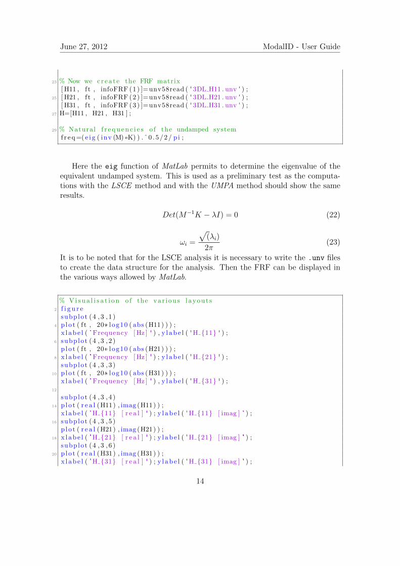
23 % Now we c r ea t e the FRF matrix[ H11 , f t , infoFRF (1) ]=unv58read ( ' 3DL H11 . unv ' ) ;
25 [ H21 , f t , infoFRF (2) ]=unv58read ( ' 3DL H21 . unv ' ) ;[ H31 , f t , infoFRF (3) ]=unv58read ( ' 3DL H31 . unv ' ) ;
27 H=[H11 , H21 , H31 ] ;
29 % Natural f r e qu en c i e s o f the undamped systemf r e q=( e i g ( inv (M) *K) ) . ˆ0 . 5/2/ p i ;
Here the eig function of MatLab permits to determine the eigenvalue of theequivalent undamped system. This is used as a preliminary test as the computa-tions with the LSCE method and with the UMPA method should show the sameresults.
Det(M−1K − λI) = 0 (22)
ωi =
√(λi)
2π(23)
It is to be noted that for the LSCE analysis it is necessary to write the .unv filesto create the data structure for the analysis. Then the FRF can be displayed inthe various ways allowed by MatLab.
% Vi s u a l i s a t i o n o f the var i ous l ayout s2 f i g u r esubplot ( 4 , 3 , 1 )
4 p lo t ( f t , 20* l og10 ( abs (H11) ) ) ;x l ab e l ( 'Frequency [Hz ] ' ) , y l ab e l ( 'H {11} ' ) ;
6 subplot ( 4 , 3 , 2 )p l o t ( f t , 20* l og10 ( abs (H21) ) ) ;
8 x l ab e l ( 'Frequency [Hz ] ' ) ; y l ab e l ( 'H {21} ' ) ;subplot ( 4 , 3 , 3 )
10 p lo t ( f t , 20* l og10 ( abs (H31) ) ) ;x l ab e l ( 'Frequency [Hz ] ' ) , y l ab e l ( 'H {31} ' ) ;
12
subplot ( 4 , 3 , 4 )14 p lo t ( r e a l (H11) , imag (H11) ) ;
x l ab e l ( 'H {11} [ r e a l ] ' ) ; y l ab e l ( 'H {11} [ imag ] ' ) ;16 subplot ( 4 , 3 , 5 )
p l o t ( r e a l (H21) , imag (H21) ) ;18 x l ab e l ( 'H {21} [ r e a l ] ' ) ; y l ab e l ( 'H {21} [ imag ] ' ) ;
subplot ( 4 , 3 , 6 )20 p lo t ( r e a l (H31) , imag (H31) ) ;
x l ab e l ( 'H {31} [ r e a l ] ' ) ; y l ab e l ( 'H {31} [ imag ] ' ) ;
14

June 27, 2012 ModalID - User Guide
22
subplot ( 4 , 3 , 7 )24 p lo t ( f t , r e a l (H11) ) ;
x l ab e l ( 'Frequency [Hz ] ' ) ; y l ab e l ( 'H {11} [ Real ] ' ) ;26 subplot ( 4 , 3 , 8 )
p l o t ( f t , r e a l (H21) ) ;28 x l ab e l ( 'Frequency [Hz ] ' ) ; y l ab e l ( 'H {21} [ Real ] ' ) ;
subplot ( 4 , 3 , 9 )30 p lo t ( f t , r e a l (H31) ) ;
x l ab e l ( 'Frequency [Hz ] ' ) ; y l ab e l ( 'H {31} [ Real ] ' ) ;32
subplot (4 , 3 , 10 )34 p lo t ( f t , imag (H11) ) ;
x l ab e l ( 'Frequency [Hz ] ' ) ; y l ab e l ( 'H {11} [ Imag ] ' ) ;36 subplot (4 , 3 , 11 )
p l o t ( f t , imag (H21) ) ;38 x l ab e l ( 'Frequency [Hz ] ' ) ; y l ab e l ( 'H {21} [ Imag ] ' ) ;
subplot (4 , 3 , 12 )40 p lo t ( f t , imag (H31) ) ;
x l ab e l ( 'Frequency [Hz ] ' ) ; y l ab e l ( 'H {31} [ Imag ] ' ) ;
15

June 27, 2012 ModalID - User Guide
Figure 3: FRFs in various formats
Before using an identification method, it is often interesting to use mode indica-tors, for checking the local range of frequency to be analyzed.
1 % now we make the check on the l o c a l f requency range[INDICATOR] = indicator mode (H) ;
3 %[ cursor1 , cur so r2 ] = p l o t i n d i c a t o r s (INDICATOR, f t ) ;
5 f i g u r e ( )subplot ( 3 , 1 , 1 )
7 p lo t ( f t , 20* l og10 (INDICATOR.ISUM) )g r id on
9 x l ab e l ( 'Frequency [Hz ] ' ) ;y l ab e l ( ' I nd i c a t o r I {Sum} [ dB ] ' ) ;
11 subplot ( 3 , 1 , 2 )p l o t ( f t , 20* l og10 (INDICATOR. ISRe ) )
13 g r id on
16
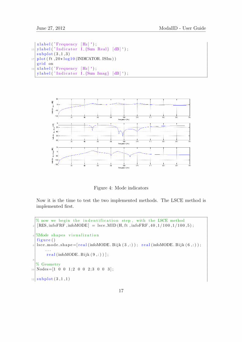
June 27, 2012 ModalID - User Guide
x l ab e l ( 'Frequency [Hz ] ' ) ;15 y l ab e l ( ' I nd i c a t o r I {Sum Real} [ dB ] ' ) ;
subplot ( 3 , 1 , 3 )17 p lo t ( f t , 20* l og10 (INDICATOR. ISIm ) )
g r id on19 x l ab e l ( 'Frequency [Hz ] ' ) ;
y l ab e l ( ' I nd i c a t o r I {Sum Imag} [ dB ] ' ) ;
Figure 4: Mode indicators
Now it is the time to test the two implemented methods. The LSCE method isimplemented first.
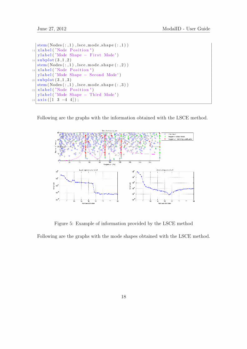
% now we begin the i n d e n t i f i c a t i o n step , with the LSCE method2 [RES, infoFRF , infoMODE ] = lsce MID (H, f t , infoFRF ,40 ,1/100 ,1/100 ,5 ) ;
4 %Mode shapes v i s u a l i z a t i o nf i g u r e ( )
6 l s ce mode shape=[ r e a l ( infoMODE . Bi jk ( 3 , : ) ) ; r e a l ( infoMODE . Bi jk ( 6 , : ) ) ;. . .r e a l ( infoMODE . Bi jk ( 9 , : ) ) ] ;
8
% Geometry10 Nodes=[1 0 0 1 ;2 0 0 2 ;3 0 0 3 ] ;
12 subplot ( 3 , 1 , 1 )
17
June 27, 2012 ModalID - User Guide
stem (Nodes ( : , 1 ) , l s ce mode shape ( : , 1 ) )14 x l ab e l ( 'Node Pos i t i on ' )
y l ab e l ( 'Mode Shape − F i r s t Mode ' )16 subplot ( 3 , 1 , 2 )
stem (Nodes ( : , 1 ) , l s ce mode shape ( : , 2 ) )18 x l ab e l ( 'Node Pos i t i on ' )
y l ab e l ( 'Mode Shape − Second Mode ' )20 subplot ( 3 , 1 , 3 )
stem (Nodes ( : , 1 ) , l s ce mode shape ( : , 3 ) )22 x l ab e l ( 'Node Pos i t i on ' )
y l ab e l ( 'Mode Shape − Third Mode ' )24 ax i s ( [ 1 3 −4 4 ] ) ;
Following are the graphs with the information obtained with the LSCE method.
Figure 5: Example of information provided by the LSCE method
Following are the graphs with the mode shapes obtained with the LSCE method.
18

June 27, 2012 ModalID - User Guide
Figure 6: Mode shapes visualization in MatLab
Then it is the time of the computation with the UMPA method.
% the second way to do the i d e n t i f i c a t i o n i s through the UMPA2 % in t h i s case we use a low order model
4 [ na t f r eq , InvCond , err , e p s i l o n ] = low order UMPA (1 ,3 ,H, f t , 2 , 2 ) ;\end{verbatim}
6
In t h i s p a r t i c u l a r case the code f o r low order model i s u t i l i z e d .There fore the denominator o f the t r a n s f e r func t i on o f the systemw i l l be o f the second order . In t h i s case a study on thes t a b i l i z a t i o n o f the modal parameters i s not p o s s i b l e as \emph{m}could vary j u s t between $1$ and $2$ .
8
%\ l s t i n p u t l i s t i n g {/SOME/PATH/low order UMPA .m}10
\begin { l s t l i s t i n g }12 % This func t i on implements the UMPA method f o r low order model .
% There fore m<=2 and in t h i s case a l s o num<=214 %
% I t takes as an input :16 % g : the FRF matrix
% w: the f requency vec to r18 % m: the numerator order
% num:20
f unc t i on [ na t f r eq , InvCond , err , e p s i l o n ] = low order UMPA(Ni ,No , g ,w,m,
19

June 27, 2012 ModalID - User Guide
num)22
[ rw , cw]= s i z e (w) ; i f rw>cw , w=w. ' ; end24 [ rg , cg ]= s i z e ( g ) ; i f rg>cg , g=g . ' ; end
26 w = [w,−w ] ;g = [ g , conj ( g ) ] ;
28
FMAX = abs (w(end)) ;30
f o r k = 0 : l ength (w)−132 W(1 :No , ( Ni*k+1) : Ni *( k+1) ) = w(1 , k+1)* ones (No , Ni ) ;
WI( 1 : Ni , ( Ni*k+1) : Ni *( k+1) ) = w(1 , k+1)* eye (Ni ) ;34
end36
OM = (1 i *W) .ˆm;38 IOM = −(1 i *WI) . ˆm;
f o r kom = m−1:−1:040 OM = [OM; ( 1 i *W) .ˆkom ] ;
IOM = [IOM;−(1 i *WI) . ˆkom ] ;42 end
44 H = g ;f o r kom = 1 :m−1
46 H = [H; g ] ;end
48
Dva = OM(No+1:end , : ) .*H;50 Dvb = IOM((m−num) *Ni+1:end , : ) ;
52 D = [ conj (Dva) ; conj (Dvb) ] ;LHS = D*D ' ;
54
rhs = −OM(1 :No , : ) .* g ;56 rhs = conj ( rhs ) ;
RHS = rhs *D ' ;58 RHS = RHS ' ;
60 AABB = LHS\RHS;AA = AABB( 1 :m*No , : ) ;
62 BB = AABB(m*No+1:end , : ) ;
64 I = eye ( (m−1)*No) ;O = ze ro s ( ( (m−1)*No) ,No) ;
66 CC = [−AA' ; I O ] ;
68 e = e i g (CC) ;n a t f r e q=abs ( e ) ;
20

June 27, 2012 ModalID - User Guide
70
% Erreur c a l c u l a t i o n72 %− Inve r s e o f cond i t i onnn ing number
InvCond = 1/cond (LHS) ;74 %− S ingu la r normal ized va lue s
[U, S ,V] = svd (LHS, 0 ) ;76 SingVals = diag (S) ;
e r r = 1/(max( SingVals ) /min ( SingVals ) ) ;78 % − o f l e a s t squares
e p s i l o n = norm(RHS−(LHS*AABB) ) ;
The high order code fails to work in this situation giving a singular matrix toworking precision at m = 3.
Hereby follows a table with the results for the Low Order computation. Its resultsare compared with the LSCE results and the theoretical ones.
Low Order UMPA LSCE Theoreticalm 1 2 2num 1 1 2Nat. freq 23.00 126.05 122.66 122.69 123.19
3.80 95.14 90.47 90.47 90.9622.99 61.54 51.86 51.87 52.35
error 1.87 E-09 1.92 E-07 6.30 E-05 5.6 E-12
invCond 5.14 E-05 1.21 E-05 1.15 E-09 1.2 E-06
It is clearly visible that the code gives better results for m = 2 and num = 2.
Through this simple example, an overview of the ModalID functionalities hasbeen illustrated. Further developments of this toolbox are previewed for the nextsix months. First of them is to solve the problems linked to the conditioning of thematrix of the system for the UMPA method, second to extend the applicability ofthis software to a general geometry given as an input through the .unv files.
21

June 27, 2012 ModalID - User Guide
References
[1] Jimin He and Zhi-Fang Fu, Modal Analysis, Butterworth- Heinemann, 2001.
[2] R. J. Allemang and A. W. Philips, The Unified Matrix Polynomial Approachto Understanding Modal Parameter Estimation, 2001.
[3] G. Kouroussis, L. Ben Fekih, C. Conti, O. Verlinden, EasyMod: A Matlab/S-ciLab toolbox for teaching modal analysis, Proceedings of the 19th InternationalCongress on Sound and Vibration, Vilnius (Lithuania), July 9-12, 2012.
22