-1-

Mode II fracture mechanics properties of solid wood measured by the three-point

eccentric end-notched flexure test

(Abbreviated title: Three-point eccentric end-notched flexure test of solid wood)

Hiroshi Yoshihara*

Faculty of Science and Engineering, Shimane University, Nishikawazu-cho 1060,

Matsue, Shimane 690-8504, Japan

* Corresponding author. Tel: +81-852-32-6508; fax: +81-852-32-6123.

E-mail address: yosihara@riko.shimane-u.ac.jp

Abstract

A three-point eccentric end-notched flexure test was conducted using specimens of

western hemlock to determine the fracture mechanics properties under Mode II

conditions while extending the crack length range for stabilising the crack propagation.

The location of the loading point was varied during the test, and the effect of the loading

point location on the initiation and propagation fracture toughness values was examined.

With the proposed method, fracture mechanics properties were appropriately obtained at

greater crack propagation lengths than in the conventional three-point end-notched

flexure test when the loading point was not extremely close to the supporting point at

the crack-free region.

Keywords: three-point eccentric end-notched flexure test; solid wood; initiation fracture

toughness; propagation fracture test; resistance curve

-2-

1. Introduction

When a crack propagates in a fibrous material such as solid wood, the fracture

toughness often increases as the crack length increases because of the existence of a

fracture process zone (FPZ) ahead of the crack tip and fibre bridgings between the crack

surfaces. Therefore, the fracture mechanics properties of fibrous materials including

solid wood have often been evaluated by a resistance curve (R-curve) that is typically

determined from the relationship between the fracture toughness and the crack length

increment during the crack propagation. A three-point end-notched flexure (3ENF) test

is a simple method for determining Mode II fracture mechanics properties such as the

initiation fracture toughness and the R-curve. In recent conventional 3ENF tests where

the load is applied to the mid-span, the fracture mechanics properties have been

frequently mathematically defined according to beam theory [1-12]. When measuring

the R-curve, however, the 3ENF test has a drawback in that the ratio of the initial crack

length to the half span should be greater than 0.7 to stabilise the crack propagation. To

obtain information on the fracture mechanics properties, it is desirable to obtain the

-3-

R-curve by stabilising the crack propagation length over a wide range. Several methods

such as stabilised end-notched flexure (SENF), end-loading shear (ELS), tapered end

notched flexure (TENF), over-notched flexure (ONF), and four-point bend end-notched

flexure (4ENF) tests have been used to stabilise crack propagation over a range wider

than the 3ENF test [13-25]. Nevertheless, there are several disadvantages in these

methods, even though they are effective at stabilising crack propagation. A SENF test

requires a servo valve-controlled testing machine that is often complicated to control

[13]. The testing data in an ELS test can often vary according to the clamping

conditions [14, 15]. The equation for deriving the fracture toughness in the TENF test is

more complicated than that of a 3ENF test [16]. In an ONF test, the effect of the

frictional forces between the crack surfaces is very significant and continuously

increases the R-curve during crack propagation [17-19]. The 4ENF test may be superior

to the aforementioned methods because of its simplicity and stability in crack

propagation [14, 20-25]. To apply a 4ENF test to solid wood, however, it is often

difficult to let the crack propagate while preventing the specimen failure by bending at

the loading point in the cracked portion without cutting deep grooves in both

-4-

side-surfaces [23, 24]. In fact, there are few examples of applying a 4ENF test to solid

wood. It is more convenient to measure the R-curve over a wide range of propagation

crack lengths through simple procedures such as equipment and specimen preparation.

In a conventional 3ENF test in which the load is applied at the mid-span of the

specimen, the range of the crack length enabling stable propagation is theoretically

restricted from 0.35 to 0.5 times the span. This range can be easily extended without

preparing any special equipment or specimens with a three-point eccentric end-notched

flexure (3EENF) test, the details of which are demonstrated below.

This study conducted a 3EENF test on western hemlock specimens to obtain an

R-curve, defined as the relationship between the propagation fracture toughness and the

propagation crack length, was obtained. Based on the R-curve, Mode II initiation

fracture toughness and represented value of the propagation fracture toughness, defined

as the averaged value of the propagation fracture toughness at the plateau portion of the

R-curve. The location of the loading point was varied in the 3EENF test, and the effect

of the location on the fracture mechanics properties described above was examined.

-5-

2. Three-point eccentric end-notched flexure analyses

Fig. 1 shows a diagram of the three-point eccentric end-notched flexure (3EENF)

test for the Mode II analysis. A specimen with a width of B, a depth in the cracked

portion of H and a crack length of a, is supported by a span with a length of 2L. As

shown in the figure, a load of P is eccentrically applied and the distance between the

loading point and the supporting point at the cracked portion is defined as c. By solving

the equation of flexure while considering the transverse shear force, the load-deflection

compliance, CL, is given as:

CL =d

P=

2L - c( )2

3a3 + 2c2L( )8ExBH

3L2+s 2L - c( )4GxyBHL

(1)

where Ex is the Young’s modulus in the length direction, which is defined as the

x-direction, Gxy is the shear modulus in the length/depth plane, which is defined as the

xy-plane, s is the Timoshenko’s shear factor which is equal to 1.2 for the beam with a

rectangular cross-section, and is the deflection at the loading point. Therefore, the

Mode II energy release rate, GII, is derived as:

GII =P2

2B

dCL

da=

9 2L - c( )2P2a2

16ExB2H 3L2

(2)

-6-

Under constant loading point deflection condition, dGII/da is derived from Eqs. (1) and

(2) as follows:

dGII

da=

9d 2 2L - c( )2a

8ExB2H 3L2C2

1-9a3

3a3 + 2c2L

æ

èçö

ø÷ (3)

To stabilise the crack propagation, dGII/da should be negative; thus,

a ³c2L

33 (4)

Based on this equation, the minimum value of a/2L, defined as amin/2L, can be

determined from the loading point location relative to the span length c/2L as follows:

amin

2L=

1

6

c

2L

æ

èçö

ø÷

2

3 (5)

The path length where the crack stably propagates, defined as ls, is derived as follows:

ls = c- amin = 2Lc

2L-

1

6

c

2L

æ

èçö

ø÷

2

3

é

ë

êê

ù

û

úú (6)

When the value of ls is large, the R-curve can be obtained over a wide range of crack

propagation lengths. Fig. 2 shows the relationship between the values of ls/2L and c/2L

obtained from Eq. (6). In a conventional 3ENF test, c = 0.5 so that ls/2L = 0.15; by

contrast, ls/2L = 0.5 in the most conventional 4ENF test [20-25]. Therefore, when the

loading point is located rightward of the mid-span, the range of the path length where

-7-

the crack stably propagates is wider than in a conventional 3ENF test, although it is

narrower than that in a 4ENF test.

In an actual fracture test, the load-deflection compliance is often greater than that

obtained by Eq. (2) because of the deformation caused by the transverse shear force,

which is the second term in Eq. (1), the fracture process zone (FPZ) induced at the

region ahead of the crack tip, and the fibre bridgings; the sample behaves as if the crack

length value is longer than the actual value. To accommodate this phenomenon, Eqs. (1)

and (2) are modified as [9]:

CL =2L - c( )

23 a+ D( )

3+ 2c2Lé

ëùû

8ExBH3L2

=2L - c( )

23aeq

3 + 2c2L( )8ExBH

3L2 (7)

GII =9 2L - c( )

2P2aeq

2

16ExB2H 3L2

(8)

where is the correction value of the crack length, and aeq is the equivalent crack length.

The influences of the transverse shear force, FPZ ahead of the crack tip, and fibre

bridgings are contained in the aeq value. Based on Eq. (7), the aeq value can be obtained

as

aeq =8ExBH

3L2CL

3 2L - c( )2

-2c2L

3

é

ëê

ù

ûú

1

3

(9)

-8-

Once the value of GII is obtained from Eq. (8), the Ex value must then be measured

with a separate test. This obstacle can be reduced when measuring the strain at a specific

point in the specimen during the fracture test. This data reduction method was originally

proposed by the author as a “compliance combination method” and it may prove

promising for the analysis of 3EENF test results [5, 9, 11, 23, 24]. According to

elementary beam theory, the longitudinal strain at a loading point x is derived as

follows:

e x =3 2L - c( )cP4ExBH

2L (10)

The x value is not influenced from the transverse shear force [9, 26]. Therefore the

load-strain compliance CS can be obtained as follows:

CS =e xP

=3 2L - c( )c4ExBH

2L (11)

By using Eqs. (7) and (11), the Young’s modulus Ex can be eliminated and the aeq value

can be obtained as follows:

aeq =2HLc

2L - c×CL

CS

-2

3c2L

æ

èçö

ø÷

1

3

(12)

By substituting Eqs. (11) and (12) into Eq. (8), GII can be obtained as

-9-

GII ==3 2L - c( )CSP

2

4BHLc

2HLc

2L - c×CL

CS

-2

3c2L

æ

èçö

ø÷

2

3

(13)

Using the compliance combination method, the GII value can be solely evaluated by the

fracture test without measuring the crack length or any elastic constants that are

implicitly contained in the load-deflection compliance CL and the load-longitudinal

strain compliances CS.

3. Finite element calculations

Two-dimensional finite element analyses (2D-FEAs) were independently

conducted on the actual fracture tests detailed below to examine the validity of the

3EENF test. The ANSYS 12 program, which is available in the Shimane University

library, was used for the FE analyses. Figs. 3(a) and (b) show the FE mesh used in the

calculations and the boundary conditions corresponding to the 3EENF test simulations.

The horizontal length of the model was 430 mm, and the model width, B, was 12 mm.

The depth of the model, 2H, was 24 mm. The model consisted of four-node plane

-10-

elements. The mesh was constructed to be finer closer to the crack tip, as shown in Fig.

3(b). The dimensions of the element at the delamination front were 0.5 and 0.5 mm in

the x- and y-directions, respectively. Table 1 presents the elastic properties used in the

present calculations, which were similar to those used in a previous study that used

spruce specimens [11]. The initial crack length a0 was determined as c - ls, thus

theoretically confirming stable crack propagation in the fracture test. Table 2 shows the

a0 value corresponding to the c/2L and c values.

The variation of the GII value under the varying crack length a was examined in the

FEAs. Table 3 shows the crack length a and the applied load P corresponding to the

loading point c. The intervals of the a value were determined to be approximately equal

to ls/5, whereas the P value was determined to correspond to the GII value in Eq. (2) as

1000 J/m2, which was approximately equal to the propagation fracture toughness GIIR

obtained in a previous study [11]. The load-deflection compliance CL was obtained from

the displacement of the node at the point behind the loading point.

The GII value was calculated using three data reduction methods: beam theory,

compliance combination, and compliance calibration methods. In the beam theory

-11-

method, the GII and aeq values were obtained by substituting the Ex and P values shown

in Tables 1 and 2 and the CL value into Eqs. (9) and (8), respectively. In the compliance

combination method, the GII and aeq values were obtained by substituting the P, CL and

CS values into Eqs. (12) and (13), respectively. The equivalent crack length

corresponding to the initial crack length a0 was defined as aeq0, and the propagation

crack length aeq was obtained as aeq = aeq - aeq0. The GII-aeq0 relationships obtained

by the beam theory and compliance combination methods were compared with each

other.

In the compliance calibration method, the CL-a relationship was regressed into the

following 4th polynomial function:

CL == A0 + A1a+ A2a2 + A3a

3 + A4a4 (14)

where A0-A4 are the parameters obtained by the regression. Using Eq. (14), the GII value

was derived as:

GII =P2

2B

dCL

da=P2

2BA1 + 2A2a + 3A3a

2 + 4A4a3( ) (15)

In the compliance calibration method, aeq was defined as a - a0, and the obtained

GII-aeq relationship was compared with those obtained from the aforementioned data

-12-

reduction methods.

In several previous studies of 3ENF, ONF, and 4ENF tests [17-24], the compliance

calibration was conducted by shifting a specimen in the support and virtually varying

the crack length. Otherwise, the specimens with various crack lengths corresponding to

the c/2L value should be prepared to obtain the CL-a relationship. In this study, however,

it was difficult to prepare specimens that satisfied these conditions. In the actual 3EENF

tests performed in this study, the compliance calibration method was not adopted for the

data reduction.

The GI and GII values were also calculated using a virtual crack closure technique

(VCCT) as follows [27]:

GI

VCCT =Fyjd yi

2BDa

GII

VCCT =Fxjd xi

2BDa

ì

í

ïï

î

ïï

(16)

where Fxj and Fy

j are the nodal forces at the crack tip node j in the x- and y-directions,

respectively, and xi and y

i are the relative displacements of the nodes i and i’, which

are located at a distance behind the crack tip, in the x- and y-directions, respectively.

Similar to the compliance calibration method, aeq was defined as a - a0, and the

-13-

obtained GII-aeq relationship was compared with the three data reduction methods.

4. Experiment

4.1. Materials

Western hemlock (Tsuga heterophylla Sarg.) lumber with a density of 463 13

kg/m3 and eight or nine annual rings contained in a radial length of 10 mm was used for

the tests. As shown in Fig. 4, the annual rings were sufficiently flat and their curvature

could thus be ignored. The lumber contained no defects such as knots or grain

distortions, and the specimens cut from it could be regarded as “small and clear.” Prior

to the test, the lumber was stored for approximately one year in a room at a constant

temperature of 20C and a relative humidity of 65% and was confirmed to be in an

air-dried condition. These conditions were maintained throughout the tests. After

conducting the 3EENF test, the specimen was oven-dried for measuring the MC of the

specimens, which were 11.7 0.2%. The Young’s modulus in the longitudinal direction,

-14-

which corresponds to Ex, was 12.6 ± 0.5 GPa, as measured by the flexural vibration tests

previously conducted by the 3EENF tests. The influence of shear deflection on the Ex

value was reduced based on Timoshenko’s vibration theory [28]. Five specimens were

used for one test condition.

4.3. Three-point eccentric end-notched flexure tests

All of the specimens were cut from the aforementioned lumber such that they

were side-matched according to the dimensions of 430 mm (longitudinal direction) 12

mm (tangential direction) 24 mm (radial direction). As previously noted, the crack

propagation must precede the bending failure in a fracture test. The bending stress is

maximised at the point where x = a and is defined as and derived as follows:

s max =3 2L - c( )Pa

2BH 2L (17)

To allow the crack to propagate while preventing the bending failure, the load P

satisfying Eq. (2) should be smaller than that satisfying Eq. (17). Therefore, the depth in

the cracked portion H should satisfy the following inequality:

-15-

H >4ExGIIR

s max

2 (18)

Equation (18) indicates that the critical value of H is independent of the location of the

loading point c/2L. Based on the GIIR and max values, which were supposed to be

approximately 1000 J/m2 and 100 MPa, the critical value of H was 6.4 mm. To firmly

enhance the crack propagation while preventing the specimen from bending failure, the

H value was determined as 12 mm in this study. In addition, the results of the FEAs

indicated that the bending rotation at the supports is smaller than 0.1 rad, so the

deformation was small enough not to consider the large bending in the 3EENF test.

The crack was produced in the longitudinal direction along the longitudinal-radial

plane, which is the so-called RL-system. Therefore, the x- and y-directions correspond

to the longitudinal and tangential directions of the wood. The crack was initially cut

with a band saw (thickness = 0.3 mm), and then extended ahead of the crack tip using a

razor blade to the initial crack length a0 shown in Table 2. Straight lines were drawn

perpendicular to the crack in the crack-free region at the intervals shown in Table 3 to

observe the approximated location of the crack tip. Two sheets of 0.05-mm-thick Teflon

were inserted between the crack surfaces to reduce the friction between the upper and

-16-

lower cantilever beams. The specimen was supported by 400-mm spans. To prevent the

specimen from indenting at the supporting point, a steel platen with a width of 30 mm

was placed between the specimen and the supporting point. A load was applied to the

point of x = c at a cross-head speed of 1 mm/min until the crack tip reached the straight

line drawn below the loading point. Fig. 5 shows the set-up of the 3EENF test. The total

testing time was approximately 15 min.

A displacement gauge was placed below the loading point to obtain the deflection

at the loading point . The longitudinal strain, x, was measured using a strain gauge

(gauge length = 2 mm; FLA-2-11, Tokyo Sokki Kenkyujo Co., Tokyo) that was bonded

at a point behind the loading point. In the bending loading, the longitudinal strain varied

in the length direction of the beam, and this variation may have affected the accuracy of

the flexural Young’s modulus value measured by the strain gauge. In addition, there

was concern that a measurement error was induced because the output from the strain

gauge was influenced by the pointwise material property variation at the region where

the strain gauge was bonded [29]. However, these concerns were reduced with a

homogeneous specimen and a short strain gauge [26, 30]. Recently, the digital image

-17-

correlation (DIC) technique is adopted for determining the Young’s modulus in a

cracked sample [31, 32]. Although the DIC technique is more complicated than bonding

a strain gauge, it is effective to characterising the elastic properties of a cracked sample,

which dominate the accuracy of the fracture mechanics properties. Comparisons

between these methods are required for a further research.

Fig. 6 shows the typical P- and P-x relationships. Similar to several previous

studies [9, 11, 23, 24], the initial load-deflection compliance CL0 and load-strain

compliance CS were determined from the initial slope of the P- and P-x relationships,

respectively, whereas the temporary load-loading point deflection compliance CL was

determined from the slope of the straight line drawn in the nonlinear region of the P-

relationship. The equivalent crack length (aeq) and propagation fracture (GIIR) values

during the crack propagation were obtained by substituting the P, CL, and CS values into

Eqs. (12) and (13), respectively. The critical load for crack propagation, defined as Pc,

was determined as that at the onset of nonlinearity in the P- relationship as shown in

Fig. 6. The initiation fracture toughness GIIc was obtained by substituting the Pc, CL0,

and CS values into Eq. (13). Similar to the FEM, the propagation crack length aeq was

-18-

obtained as aeq = aeq - aeq0, and the R-curve was obtained as the GIIR-aeq relationship.

In addition, the GIIR values were averaged, and the representative value of propagation

fracture toughness, defined as GIIR, was obtained. In this study, the plateau region of

the R-curve was defined as that between the maximal and minimal values of GIIR before

the continuous increasing of the GIIR value, the details of which are described below.

The obtained GIIc and GIIR values were compared with each other, and the effect of the

loading location was examined.

5. Results and discussion

5.1. Finite element calculations

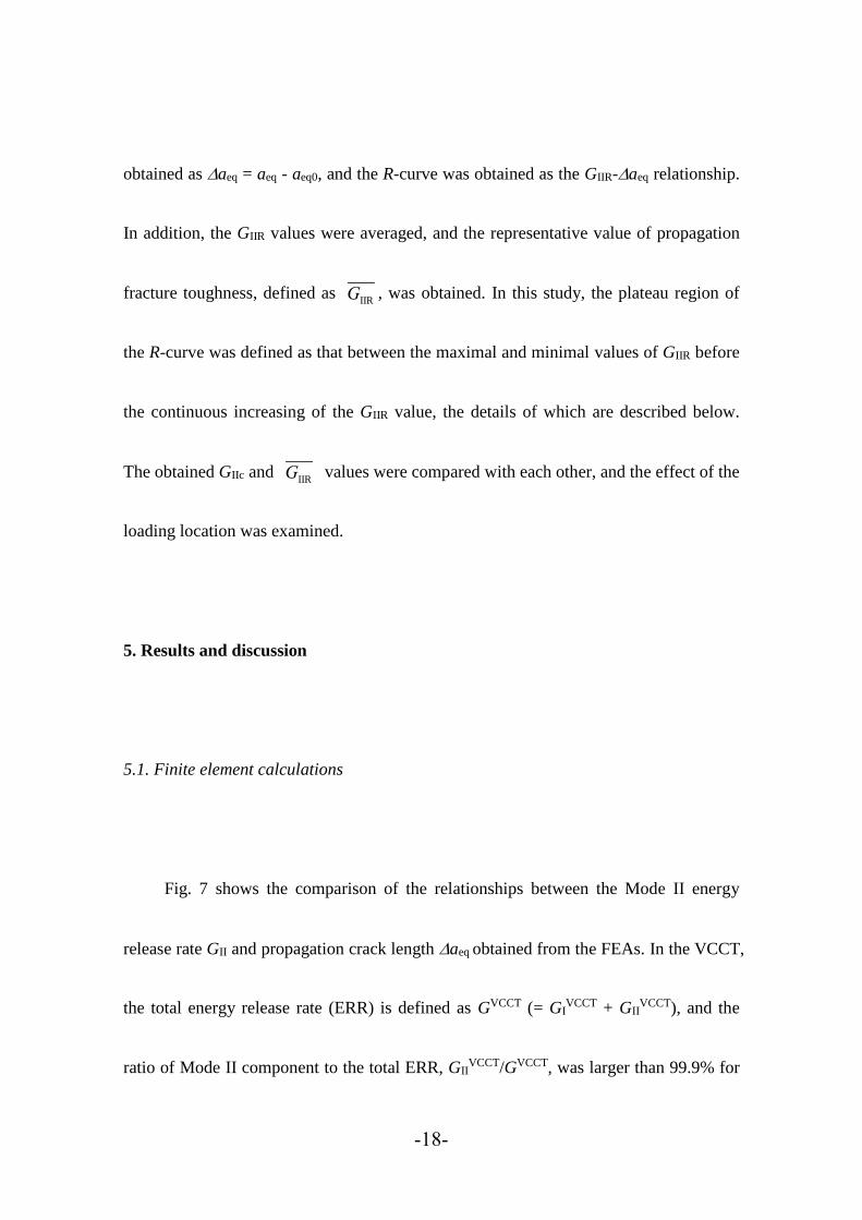
Fig. 7 shows the comparison of the relationships between the Mode II energy

release rate GII and propagation crack length aeq obtained from the FEAs. In the VCCT,

the total energy release rate (ERR) is defined as GVCCT (= GIVCCT + GII

VCCT), and the

ratio of Mode II component to the total ERR, GIIVCCT/GVCCT, was larger than 99.9% for

-19-

all analysis results. Therefore, the 3EENF tests conducted in this study could be

regarded to be a rather pure Mode II condition. All of the GII values obtained by the data

reduction methods and the VCCT were greater than 1000 J/m2, which was obtained by

substituting the a and P values listed in Table 3 into Eq. (2), because of the shear

deformation and the crack tip rotation ahead of the crack tip [2-12]. The GII values

obtained from the beam theory and compliance combination methods were greater than

those obtained from the VCCT. These discrepancies were enhanced as the c/2L value

increased. In contrast, the GII value obtained from the compliance calibration method,

which was not adopted in the actual fracture test in this study, coincided well with that

obtained from the VCCT.

There were discrepancies in the FEA results between the GII values obtained from

the different data reduction methods. In conventional 3ENF tests conducted in a

previous study [5], however, these discrepancies were not so significant. In the FEAs

conducted in this study, the softening behaviour due to the fracture process zone (FPZ)

ahead of the crack tip was not taken into account, although it had been considered in the

analyses of previously conducted 3ENF tests [6, 7, 34-37]. If the effect of the FPZ is

-20-

considered, then the FEA results may be different from those obtained in this study.

Further research should be conducted to reveal the validity of these data reduction

methods in more detail.

Recently, Moutou Pitti et al. [38] adopted the M-integral for analysing the crack

growth in orthotropic material like solid wood based on the approach by FEM.

Although the M-integral is often complicated than the data reduction methods based on

the compliance, they may be effective for characterising the fracture properties of solid

wood. In addition, as described previously, there are several examples conducting the

crack propagation simulations by FEA for characterising the fracture mechanics

properties while the FPZ and fibre bridgings are taken into account [6, 7, 35-38].

Further researches are also required to examine the applicability of these novel methods

on the 3EENF test.

5.2. Three-point end-notched flexure tests

Fig. 8 shows the R-curves obtained in the 3EENF tests under different loading

-21-

point locations. As shown in this figure, the crack wholly propagated stably during the

test in the range of propagation crack length. It was revealed from the FEA and actual

fracture test results that the GIIR-aeq relationships obtained from the beam theory and

compliance combination methods coincided well with each other. Therefore, the

R-curves in Fig. 7 were obtained based solely on the compliance combination method.

Similar to the results shown in several previous studies, the R-curve initially increased

steeply and then displayed a plateau region. After the plateau region, the R-curve

increased again because of the concentration of stress around the loading point and the

confinement of the FPZ [11, 36, 39]. In the conventional 3ENF test, the range of the ls

value was restricted because of the initial crack length, which should be longer than

0.7L, and the confinement of the FPZ when the crack tip was close to the loading point.

However, the range of aeq in the R-curve can be extended by conducting the 3EENF

test. Nevertheless, the GIIR values in the plateau region of the specimens with c/2L

values of 0.8 and 0.9 were often greater than the others. In addition, the variation of the

GIIR value was more significant in these conditions. As shown in the FEA results in Fig.

7, the greater GIIR values in these conditions may be due to the compliance combination

-22-

method adopted in this study. In addition, the influence of the frictional force and fibre

bridgings between the cracked surfaces may be significant for the R-curve behaviours of

the specimens with c/2L values of 0.8 and 0.9, the cracked surfaces of which are

relatively large. Therefore, the resistance against the crack propagation may be induced

under these conditions. Further research should also be conducted to reveal these

phenomena in more detail.

Fig. 9 shows the initiation and propagation fracture toughness values, GIIc and

GIIR, respectively, corresponding to the location of the loading point c/2L. The GIIc

values were constant independent of the c/2L. In contrast, the GIIR values of the

specimens with c/2L = 0.8 and 0.9 were significantly larger than the others, and the

variation of the GIIR value was significant in these c/2L ranges. As demonstrated in

several previous studies, Mode II fracture mechanics behaviours can be obtained from

the conventional 3ENF test, where c/2L = 0.5 [1-12]. Because the GIIc and GIIRvalues

in c/2L = 0.5-0.7 are close to each other, the fracture mechanics properties obtained in

these conditions are thought to be valid. In particular, the aeq value is approximately

twice as high in the condition of c/2L = 0.7 than in the conventional 3ENF test condition

-23-

(c/2L = 0.5). In contrast, the 3EENF test conditions of c/2L = 0.8 and 0.9 should be

examined in more detail, although it is feasible to extend the propagation crack length

under these conditions.

As described above, the sample behaves as if the crack length value is longer than

the actual value because of the deformation caused by the transverse shear force, the

FPZ, and the fibre bridgings. Considering this phenomenon, the value was evaluated

from the following equation:

D = aeq0 - a0 (18)

Fig. 10 shows the value corresponding to the location of the loading point c/2L. The

value was approximately 35 mm. Morel et al. pointed out that the length of the FPZ

reaches approximately several centimetres [39]. The value contains the effects of

deformation caused by the transverse shear force and the fibre bridgings as well as the

FPZ, so it may not be comparable to the results obtained by Morel et al. As described

above, however, it is reasonable that the large part of the value is because of the

length of the FPZ, which induces the increase of the R-curve at the end of the fracture

test.

-24-

6. Conclusions

Three-point end-notched flexure (3EENF) tests were conducted using specimens

of western hemlock to determine the Mode II fracture mechanics properties, including

the resistance curve (R-curve), initiation fracture toughness, and propagation fracture

toughness. These properties were obtained using a compliance combination method as

the data reduction method. In addition to the fracture tests, finite element analyses

(FEAs) were conducted and the validity of the 3EENF test methods were also

examined.

The FEA results demonstrated that the discrepancies of the GII values obtained

from the data reduction methods (beam theory and compliance combination methods)

and those obtained from the VCCT were more pronounced when the loading point

approached the supporting point at the crack-free region.

For all of the specimens, the R-curve initially increased steeply, then displayed a

plateau region, and finally increased again due to the concentration of stress around the

-25-

loading point and the confinement of the FPZ. The initiation fracture toughness GIIc was

not dependent on the location of the loading point. In contrast, the GIIR values in the

plateau region of the tests under the c/2L conditions of 0.8 and 0.9 were often greater

than those under the c/2L conditions of 0.5-0.7. This phenomenon affected the

represented value of propagation fracture toughness GIIR, which demonstrated a

tendency similar to that of GIIR.

Based on the summarized results obtained in this study, fracture mechanics

properties can be appropriately obtained from a 3EENF test when the loading point is

not extremely close to the supporting point at the crack-free region.

Acknowledegments: This work was supported in part by a Grant-in-Aid for Scientific

Research (C) (No. 24580246) of the Japan Society for the Promotion of Science.

References

[1] Barrett JD, Foschi RO. Mode II stress-intensity factors for cracked wood beams.

-26-

Engrg Fract Mech 1977; 9: 371-8.

[2] Yoshihara H, Ohta M. Measurement of mode II fracture toughness of wood by the

end-notched flexure test. J Wood Sci 2000; 46: 273-8.

[3] Yoshihara H. Influence of span/depth ratio on the measurement of mode II fracture

toughness of wood by end-notched flexure test. J Wood Sci 2001; 47: 8-12.

[4] Yoshihara H. Resistance curve for the mode II fracture toughness of wood obtained

by end-notched flexure test under the constant loading point displacement

condition. J Wood Sci 2003; 49 (3): 210-5.

[5] Yoshihara H. Mode II initiation fracture toughness analysis for wood obtained by

3-ENF test. Compos Sci Technol 2005; 65: 2198-207.

[6] Silva MAL, de Moura MFSF, Morais JJL. Numerical analysis of the ENF test for

mode II wood fracture. Composites A 2006; 37: 1334-44.

[7] de Moura MFSF, Silva MAL, de Morais AB, Morais JJL. Equivalent crack based

mode II fracture characterization of wood. Engrg Fract Mech 2006; 73: 978-93.

[8] de Moura MFSF, Silva MAL, Morais JJL, de Morais AB, Lousada JJL. Data

reduction scheme for measuring GIIc of wood in end-notched flexure (ENF) tests.

-27-

Holzforschung 2009; 63: 99-106.

[9] Yoshihara H, Satoh A. Shear and crack tip deformation correction for the double

cantilever beam and three-point end-notched flexure specimens for mode I and mode

II fracture toughness measurement of wood. Engrg Fract Mech 2009; 76: 335-46.

[10] Arrese A, Carbajal N, Vargas G, Mujika F. A new method for determining mode II

R-curve by the end-notched flexure test. Engrg Fract Mech 2010; 77: 51-70.

[11] Yoshihara H. Initiation and propagation fracture toughness of solid wood under the

mixed Mode I/II condition examined by mixed-mode bending test. Engrg Fract

Mech 2013; 104: 1-15.

[12] Rhême M, Botsis J, Cugnoni J, Navi P. Influence of the moisture content on the

fracture characteristics of welded wood joint. Part 2: Mode II fracture.

Holzforschung 2013; 67: 755-61.

[13] Kageyama K, Kikuchi M, Yanagisawa N. Stabilized end notched flexure test.

Characterization of mode II interlaminar crack growth. ASTM STP 1110 1992:

210-25.

[14] Davies P, Sims GD, Blackman BRK, Brunner AJ, Kageyama K, Hojo M, Tanaka K,

-28-

Murri G, Rousseau C, Gieseke B, Martin RH. Comparison of test configuration for

the determination of GIIc: Results from an international round robin. Plast Rubber

Compos 1999; 28: 432-7.

[15] Silva MAL, Morais JJL, de Moura MFSF, Lousada JL. Mode II wood fracture

characterization using the ELS test. Engrg Fract Mech 2007; 74: 2133-47.

[16] Qiao PZ, Wang JL, Davalos JF. Analysis of tapered ENF specimen and

characterization of bonded interface fracture under Mode-II loading. Int J Solid

Struct 2003; 40: 1865-84.

[17] Wang J, Qiao PZ. Novel beam analysis of end notched flexure specimen for

mode-II fracture. Eng Fract Mech 2004; 71: 219-31.

[18] Kutnar A, Kamke FA, Nairn JA, Senek M. Mode II fracture behavior of bonded

viscoelastic thermal compressed wood. Wood Fiber Sci 2008; 40: 362-73.

[19] Wang WX, Nakata M, Takao Y, Matsubara T. Experimental investigation on test

methods for mode II interlaminar fracture testing of carbon fiber reinforced

composites. Composites A. 2009; 40: 1447-55.

[20] Martin RH, Davidson BD. Mode II fracture toughness evaluation using four point

-29-

bend, end notched flexure test. Plast Rubber Compos. 1999; 28: 401–6.

[21] Schuecker C, Davidson BD. Evaluation of the accuracy of the four-point bend

end-notched flexure test for mode II delamination toughness determination.

Compos Sci Technol. 2000; 60: 2137-46.

[22] Davidson BD, Sun X. Effects of friction, geometry, and fixture compliance on the

perceived toughness from three-and four-Point bend end-notched flexure tests. J

Reinforced Plast Compos 2005; 24: 1611-28.

[23] Yoshihara H. Mode II R-curve of wood measured by 4-ENF test. Eng Fract Mech

2004; 71: 2065-7.

[24] Yoshihara H. Theoretical analysis of 4-ENF tests for mode II fracturing in wood by

finite element method. Engrg Fract Mech 2008; 75: 290-296.

[25] Qiao P, Zhang L, Chen F, Chen Y, Shan L. Fracture characterization of Carbon

fiber-reinforced polymer-concrete bonded interfaces under four-point bending.

Engrg Fract Mech 2011; 78: 1247-63.

[26] Yoshihara H, Kubojima Y, Ishimoto T. Several examinations on the static bending

test methods of wood using todomatsu (Japanese fir). Forest Prod J 2003; 52(2):

-30-

39-44.

[27] Krueger R. The virtual crack closure technique: History, approach and applications.

NASA CR-2002-211628; 2002.

[28] Yoshihara H. Examination of the specimen configuration and analysis method in

the flexural and longitudinal vibration tests of solid wood and wood-based

materials. Forest Prod J 2012; 62(3): 191-200.

[29] Yadama V, Davalos JF, Loferski JR, Holzer SM. Selecting a gauge length to

measure parallel-to-grain strain in southern pine. Forest Prod J 1991; 41(10): 65-8.

[30] Yoshihara H, Tsunematsu S. Feasibility of estimation methods for measuring

Young’s modulus of wood by three-point bending test. Mater Struct 2006; 39:

29-36.

[31] Dubois F, Méité M, Pop O, Absi J. Characterization of timber fracture using the

Digital Image Correlation technique and Finite Element Method. Engrg Fract Mech

2012; 96: 107-21.

[32] Méité M, Pop O, Dubois F, Absi J. Characterization of mixed-mode fracture based

on a complementary analysis by means of full-field optical and finite element

-31-

approaches. Int J Fract 2013; 180: 41-52.

[33] Morel S, Lespine C, Coureau JL, Planas J, Dourado N. Bilinear softening

parameters and equivalent LEFM R-curve in quasibrittle failure. Int J Solid Struct

2010; 47: 837-50.

[34] Dourado N, Morel S, de Moura MFSF, Valentin G, Morais J. Comparison of

fracture properties of two wood species through cohesive crack simulations.

Composites A 2008; 39: 415-27.

[35] Dourado N, Morel S, de Moura MFSF, Valentin G, Morais J. A new data reduction

scheme for mode I wood fracture characterization using the double cantilever beam

test. Engrg Fract Mech 2008; 75: 3852-65.

[36] de Moura MFSF, Dourado N, Morais JJL, Pereira FAM. Numerical analysis of the

ENF and ELS tests applied to mode II fracture characterization of cortical bone

tissue. Fatigue Fract Engrg Mater Struct 2011; 34: 149-58.

[37] Lartigau J, Coureau JL, Morel S, Galimard P, Maurin E. Mixed mode fracture of

glued-in rods in timber structures. A new approach based on equivalent LEFM. Int

J Fract 2014; in press (online available).

-32-

[38] Moutou Pitti R, Dubois F, Petit C, Sauvat N, Pop O. A new M-integral parameter

for mixed-mode crack growth in orthotropic viscoelastic material. Engrg Fract

Mech 2008; 75: 4450-65.

[39] Coureau JL, Morel S, Dourado N. Cohesive zone model and quasibrittle failure of

wood: A new light on the adapted specimen geometries for fracture tests. Engrg

Fract Mech 2013; 109: 328-40.

-33-

Figure captions

Fig. 1. Schematic diagram of the three-point eccentric end-notched flexure (3EENF)

test.

Fig. 2. Relationship between the ls/2L and c/2L values.

Fig. 3. The finite element (FE) meshes used in the simulations. Unit = mm. a and P

values corresponding to the length between the left supporting point and loading

point c are listed in Table 3.

Fig. 4. Photograph of cross-section of the material used in this experiment

Fig. 5. Set-up of the three-point end-notched flexure (3EENF) test.

Fig. 6. Load-deflection at the loading point, load-longitudinal strain relationships and

the definitions of critical load for crack propagation Pc, temporary load-loading

point deflection compliance CL, initial load-loading point deflection compliance

CL0, and load-longitudinal strain compliance CS.

Fig. 7. Relationships between the Mode II energy release rate GII and propagation crack

length aeq obtained from the FEAs.

Fig. 8. Resistance curves (R-curves) obtained in the 3EENF tests under different loading

locations. Data reduction was conducted based on the compliance combination

method.

Fig. 9. Initiation and representative propagation fracture toughness values, GIIc and

GIIR, respectively, corresponding to the location of the loading point c/2L. The

results are the average ± SD.

Fig. 10. Correction value of crack length calculated from the compliance combination

method corresponding to the location of the loading point c/2L. The results are

the average ± SD.

-34-

Table 1. Elastic constants used for the finite element analysis and data reduction.

Ex (GPa) Ey (GPa) Gxy (GPa) xy

16.0 0.8 0.73 0.10 0.61 0.04 0.49

Results are the average SD. x- and y-directions correspond to the longitudinal and

tangential directions of sitka spruce data obtained in a previous study [10].

-35-

Table 2. The distance between the loading point and left supporting point, c, the

maximum length for stabilising the crack propagation, ls, and initial crack length a0

corresponding to the location of the loading point, c/2L.

c/2L c (mm) ls/2L ls (mm) a0 (mm)

0.5 200 0.153 61 139

0.6 240 0.209 84 156

0.7 280 0.266 106 174

0.8 320 0.326 130 190

0.9 360 0.387 155 205

a0 was determined as c - ls.

-36-

Table 3. Applied load P corresponding to the crack length a in the FEAs.

c = 200 mm c = 240 mm c = 280 mm c = 320 mm c = 360 mm

a (mm) P (N) a (mm) P (N) a (mm) P (N) a (mm) P (N) a (mm) P (N)

139 605 156 674 174 806 190 1107 205 2052

151 556 173 609 195 718 216 974 236 1782

163 515 190 555 216 648 242 869 267 1575

176 479 206 510 238 590 268 785 298 1412

188 448 223 471 259 542 294 715 329 1279

200 421 240 438 280 501 320 657 360 1168

-37-

Fig. 1. Schematic diagram of the three-point eccentric end-notched flexure (3EENF) test.

L and R represent the longitudinal and radial directions, respectively.

P

2L

c

a

2H

x (L)

y (R)

LVDT

-38-

Fig. 2. Relationship between the ls/2L and c/2L values.

c/2L

l s/2

L

-39-

Fig. 3. The finite element (FE) meshes used in the simulations. Unit = mm. a and P

values corresponding to the length between the left supporting point and loading

point c are listed in Table 3.

1.1

Delamination front

1

A B

A' B' C

P

(a) Whole mesh of 3EENF test simulation

(b) Detail around the delamination front

Δα = 0.5

0.1

Delamination

15

a

400 - c 15c

ls

-40-

Fig. 4. Photograph of cross-section of the material used in this experiment

-41-

Fig. 5. Set-up of the three-point end-notched flexure (3EENF) test.

Specimen

Steel platen

Strain gauge

LVDT

Loading nose

Steel platen

Teflon film

-42-

Fig. 6. Load-deflection at the loading point, load-longitudinal strain relationships and

the definitions of critical load for crack propagation Pc, temporary load-loading point

deflection compliance CL, initial load-loading point deflection compliance CL0, and

load-longitudinal strain compliance CS.

-43-

Fig. 7. Relationships between the Mode II energy release rate GII and propagation

crack length aeq obtained from the FEAs.

GII (

J/m

2)

GII (

J/m

2)

GII (

J/m

2)

GII (

J/m

2)

GII (

J/m

2)

c/2L = 0.5 c/2L = 0.6 c/2L = 0.7

c/2L = 0.8 c/2L = 0.9

Propagation crack length Δaeq (mm) Propagation crack length Δaeq (mm)

Propagation crack length Δaeq (mm) Propagation crack length Δaeq (mm) Propagation crack length Δaeq (mm)

: VCCT : Beam theory : Compliance combination : Compliance calibration : Eq. (2)

-44-

Fig. 8. Resistance curves (R-curves) obtained in the 3EENF tests under different loading

locations. Data reduction was conducted based on the compliance combination method.

GII

R (

J/m

2)

GII

R (

J/m

2)

GII

R (

J/m

2)

GII

R (

J/m

2)

GII

R (

J/m

2)

c/2L = 0.5 c/2L = 0.6 c/2L = 0.7

c/2L = 0.8 c/2L = 0.9

Propagation crack length Δaeq (mm) Propagation crack length Δaeq (mm)

Propagation crack length Δaeq (mm) Propagation crack length Δaeq (mm) Propagation crack length Δaeq (mm)

-45-

Fig. 9. Initiation and representative propagation fracture toughness values, GIIc and

GIIR, respectively, corresponding to the location of the loading point c/2L. The results

are the average ± SD.

-46-

Fig. 10. Correction value of crack length calculated from the compliance combination

method corresponding to the location of the loading point c/2L. The results are the

average ± SD.

Location of the loading point c/2L

Δ (

mm

)