model-based machine learning for physical-layer
TRANSCRIPT
Model-Based Machine Learning for Physical-LayerCommunication over Optical Fiber
Christian Häger
Department of Electrical Engineering, Chalmers University of Technology, Sweden
Summer School on “AI for Optical Networks &Neuromorphic Photonics for AI Acceleration”
September 6, 2021
Machine Learning Physics-Based Models Learned DBP Polarization Effects Conclusions
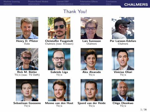
Thank You!
Henry D. PfisterDuke
Christoffer FougstedtChalmers (now: Ericsson)
Lars SvenssonChalmers
Per Larsson-EdeforsChalmers
Rick M. BütlerTU/e (now: TU Delft)
Gabriele LigaTU/e
Alex AlvaradoTU/e
Vinícius OliariTU/e
Sebastiaan GoossensTU/e
Menno van den HoutTU/e
Sjoerd van der HeideTU/e
Chigo OkonkwoTU/e
1 / 36

Machine Learning Physics-Based Models Learned DBP Polarization Effects Conclusions
Motivation and Challenges
Source: Cisco 2017
• The COVID-19 pandemic has highlighed the importance of our globalcommunication infrastructure
• Data traffic has been and will continue to grow exponentially
• Simply scaling current technology is not sustainable: fiber infrastructurewould consume all world-wide electricity within less than 10 years
2 / 36

Machine Learning Physics-Based Models Learned DBP Polarization Effects Conclusions
Motivation and Challenges
Source: Cisco 2017
Higher data rates?
More energy efficiency?
New functionalities?
• The COVID-19 pandemic has highlighed the importance of our globalcommunication infrastructure
• Data traffic has been and will continue to grow exponentially
• Simply scaling current technology is not sustainable: fiber infrastructurewould consume all world-wide electricity within less than 10 years
How can machine learning (ML) be used productively in communications toimprove future systems?
2 / 36
Machine Learning Physics-Based Models Learned DBP Polarization Effects Conclusions
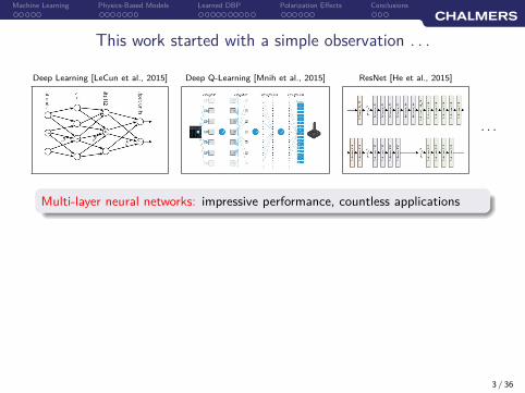
This work started with a simple observation . . .
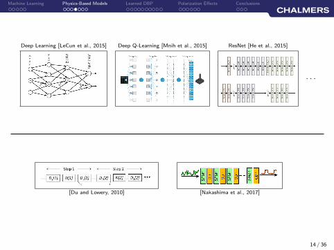
Deep Learning [LeCun et al., 2015] Deep Q-Learning [Mnih et al., 2015] ResNet [He et al., 2015]
· · ·
Multi-layer neural networks: impressive performance, countless applications
3 / 36
Machine Learning Physics-Based Models Learned DBP Polarization Effects Conclusions
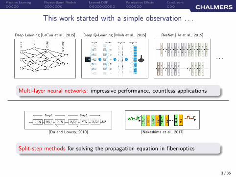
This work started with a simple observation . . .
Deep Learning [LeCun et al., 2015] Deep Q-Learning [Mnih et al., 2015] ResNet [He et al., 2015]
· · ·
Multi-layer neural networks: impressive performance, countless applications
[Du and Lowery, 2010] [Nakashima et al., 2017]
Split-step methods for solving the propagation equation in fiber-optics
3 / 36

Machine Learning Physics-Based Models Learned DBP Polarization Effects Conclusions
Agenda
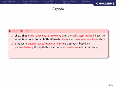
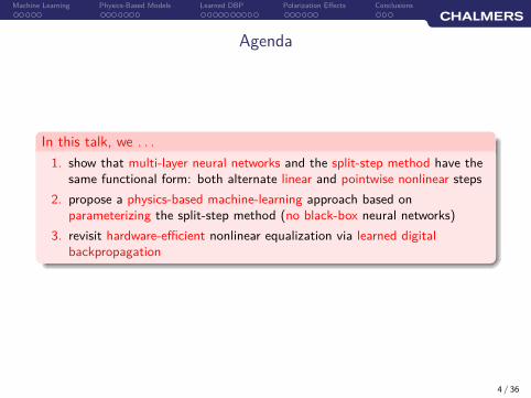
In this talk, we . . .
4 / 36

Machine Learning Physics-Based Models Learned DBP Polarization Effects Conclusions
Agenda
In this talk, we . . .
1. show that multi-layer neural networks and the split-step method have thesame functional form: both alternate linear and pointwise nonlinear steps
4 / 36
Machine Learning Physics-Based Models Learned DBP Polarization Effects Conclusions
Agenda
In this talk, we . . .
1. show that multi-layer neural networks and the split-step method have thesame functional form: both alternate linear and pointwise nonlinear steps
2. propose a physics-based machine-learning approach based onparameterizing the split-step method (no black-box neural networks)
3. revisit hardware-efficient nonlinear equalization via learned digitalbackpropagation
4 / 36
Machine Learning Physics-Based Models Learned DBP Polarization Effects Conclusions
Outline
1. Machine Learning and Neural Networks for Communications
2. Physics-Based Machine Learning for Fiber-Optic Communications
3. Learned Digital Backpropagation
4. Polarization-Dependent Effects
5. Conclusions
5 / 36
Machine Learning Physics-Based Models Learned DBP Polarization Effects Conclusions
Outline
1. Machine Learning and Neural Networks for Communications
2. Physics-Based Machine Learning for Fiber-Optic Communications
3. Learned Digital Backpropagation
4. Polarization-Dependent Effects
5. Conclusions
6 / 36

Machine Learning Physics-Based Models Learned DBP Polarization Effects Conclusions
Supervised Learning
y1
yn
z1
zm
fθ(y)
parametersto be optimized/learned
bbb
bbb
0.010.920.010.000.000.010.000.040.010.01
z
bbb
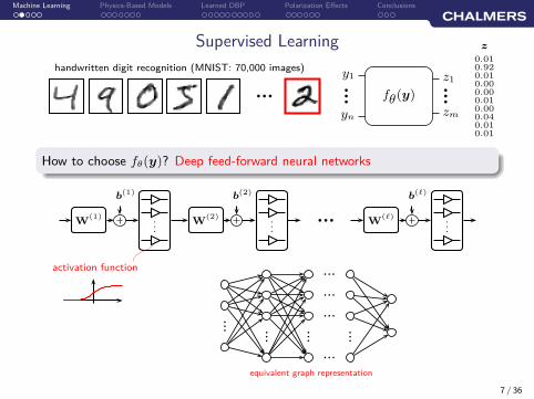
handwritten digit recognition (MNIST: 70,000 images)
28 × 28 pixels =⇒ n = 784
7 / 36
Machine Learning Physics-Based Models Learned DBP Polarization Effects Conclusions
Supervised Learning
y1
yn
z1
zm
fθ(y)bbb
bbb
0.010.920.010.000.000.010.000.040.010.01
z
bbb
handwritten digit recognition (MNIST: 70,000 images)
How to choose fθ(y)? Deep feed-forward neural networks
W(1)
b(1)
...
activation function
W(2)
b(2)
...bbb
W(ℓ)
b(ℓ)
...
bb
b
bb
bbb
bbb
b
bb b
bb b
bb b
bb b
equivalent graph representation
7 / 36
Machine Learning Physics-Based Models Learned DBP Polarization Effects Conclusions
Supervised Learning
y1
yn
z1
zm
fθ(y)bbb
bbb
0.010.920.010.000.000.010.000.040.010.01
z
bbb
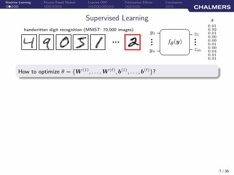
handwritten digit recognition (MNIST: 70,000 images)
How to optimize θ = {W (1), . . . , W (ℓ), b(1), . . . , b(ℓ)}?
7 / 36
Machine Learning Physics-Based Models Learned DBP Polarization Effects Conclusions
Supervised Learning
y1
yn
z1
zm
fθ(y)bbb
bbb
0100000000
x
0.010.920.010.000.000.010.000.040.010.01
z
bbb
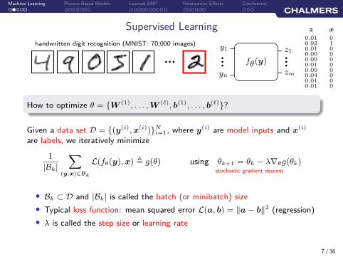
handwritten digit recognition (MNIST: 70,000 images)
How to optimize θ = {W (1), . . . , W (ℓ), b(1), . . . , b(ℓ)}?
Given a data set D = {(y(i), x(i))}Ni=1, where y(i) are model inputs and x(i)
are labels, we iteratively minimize
1
|Bk|
∑
(y,x)∈Bk
L(fθ(y), x) , g(θ) using θk+1 = θk − λ∇θg(θk)
• Bk ⊂ D and |Bk| is called the batch (or minibatch) size
• Typical loss function: mean squared error L(a, b) = ‖a − b‖2 (regression)
• λ is called the step size or learning rate
7 / 36
stochastic gradient descent

Machine Learning Physics-Based Models Learned DBP Polarization Effects Conclusions
Why Deep Models?
Many possible answers
One advantage is complexity: deep computation graphs tend to be moreparameter efficient than shallow graphs [Lin et al., 2017]
∗ ≈
= zero coefficient = nonzero coefficient
∗ ∗ ∗
• Sparsity can emerge due to (approximate) factorization (even for linearmodels, e.g., FFT)
• Deep computation graphs allow for very simple elementary steps
• Deep models typically have many “good” parameter configurations thatare close to each other =⇒ robustness to, e.g., quantization noise
8 / 36
Machine Learning Physics-Based Models Learned DBP Polarization Effects Conclusions
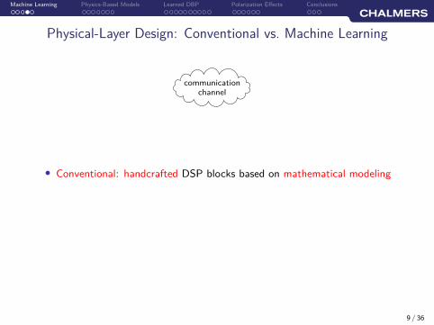
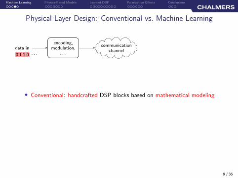
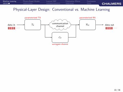
Physical-Layer Design: Conventional vs. Machine Learning
communicationchannel
• Conventional: handcrafted DSP blocks based on mathematical modeling
9 / 36
Machine Learning Physics-Based Models Learned DBP Polarization Effects Conclusions
Physical-Layer Design: Conventional vs. Machine Learning
communicationchannel
data inencoding,
modulation,. . .0 1 1 0 · · ·
• Conventional: handcrafted DSP blocks based on mathematical modeling
9 / 36
Machine Learning Physics-Based Models Learned DBP Polarization Effects Conclusions
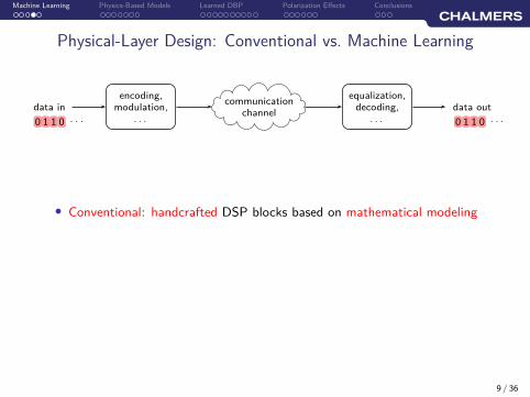
Physical-Layer Design: Conventional vs. Machine Learning
communicationchannel
data inencoding,
modulation,. . .0 1 1 0 · · ·
data out
0 1 1 0 · · ·
equalization,decoding,
. . .
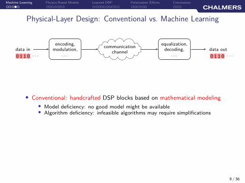
• Conventional: handcrafted DSP blocks based on mathematical modeling
9 / 36
Machine Learning Physics-Based Models Learned DBP Polarization Effects Conclusions
Physical-Layer Design: Conventional vs. Machine Learning
communicationchannel
data inencoding,
modulation,. . .0 1 1 0 · · ·
data out
0 1 1 0 · · ·
equalization,decoding,
. . .
• Conventional: handcrafted DSP blocks based on mathematical modeling
• Model deficiency: no good model might be available• Algorithm deficiency: infeasible algorithms may require simplifications
9 / 36

Machine Learning Physics-Based Models Learned DBP Polarization Effects Conclusions
Physical-Layer Design: Conventional vs. Machine Learning
communicationchannel
data inencoding,
modulation,. . .0 1 1 0 · · ·
data out
0 1 1 0 · · ·
parameterized RX
Rθ
• Conventional: handcrafted DSP blocks based on mathematical modeling
• Model deficiency: no good model might be available• Algorithm deficiency: infeasible algorithms may require simplifications
• Use function approximators and learn parameter configurations θ from data
[Shen and Lau, 2011], Fiber nonlinearity compensation using extreme learning machine for DSP-based . . . , (OECC)[Giacoumidis et al., 2015], Fiber nonlinearity-induced penalty reduction in CO-OFDM by ANN-based . . . , (Opt. Lett.)
. . .
9 / 36
Machine Learning Physics-Based Models Learned DBP Polarization Effects Conclusions
Physical-Layer Design: Conventional vs. Machine Learning
communicationchannel
data in
0 1 1 0 · · ·
parameterized TX
Tθ data out
0 1 1 0 · · ·
parameterized RX
Rθ
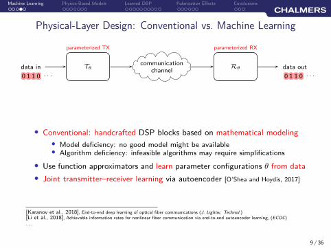
• Conventional: handcrafted DSP blocks based on mathematical modeling
• Model deficiency: no good model might be available• Algorithm deficiency: infeasible algorithms may require simplifications
• Use function approximators and learn parameter configurations θ from data
• Joint transmitter–receiver learning via autoencoder [O’Shea and Hoydis, 2017]
[Karanov et al., 2018], End-to-end deep learning of optical fiber communications (J. Lightw. Technol.)[Li et al., 2018], Achievable information rates for nonlinear fiber communication via end-to-end autoencoder learning, (ECOC)
. . .
9 / 36

Machine Learning Physics-Based Models Learned DBP Polarization Effects Conclusions
Physical-Layer Design: Conventional vs. Machine Learning
communicationchannel
data in
0 1 1 0 · · ·
parameterized TX
Tθ data out
0 1 1 0 · · ·
parameterized RX
Rθ
Cθ
surrogate channel
• Conventional: handcrafted DSP blocks based on mathematical modeling
• Model deficiency: no good model might be available• Algorithm deficiency: infeasible algorithms may require simplifications
• Use function approximators and learn parameter configurations θ from data
• Joint transmitter–receiver learning via autoencoder [O’Shea and Hoydis, 2017]
• Surrogate channel models for gradient-based TX training
[O’Shea et al., 2018], Approximating the void: Learning stochastic channel models from observation with variational GANs, (arXiv)[Ye et al., 2018], Channel agnostic end-to-end learning based communication systems with conditional GAN, (arXiv)
. . .
9 / 36
Machine Learning Physics-Based Models Learned DBP Polarization Effects Conclusions
Physical-Layer Design: Conventional vs. Machine Learning
communicationchannel
data in
0 1 1 0 · · ·
parameterized TX
Tθ data out
0 1 1 0 · · ·
parameterized RX
Rθ
Cθ
surrogate channel
10 / 36
Machine Learning Physics-Based Models Learned DBP Polarization Effects Conclusions
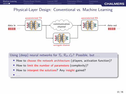
Physical-Layer Design: Conventional vs. Machine Learning
communicationchannel
data in
0 1 1 0 · · ·
parameterized TX
data out
0 1 1 0 · · ·
parameterized RX
surrogate channel
Using (deep) neural networks for Tθ, Rθ, Cθ? Possible, but . . .
• How to choose the network architecture (#layers, activation function)?
• How to limit the number of parameters (complexity)?
• How to interpret the solutions? Any insight gained?
• . . .
10 / 36
Machine Learning Physics-Based Models Learned DBP Polarization Effects Conclusions
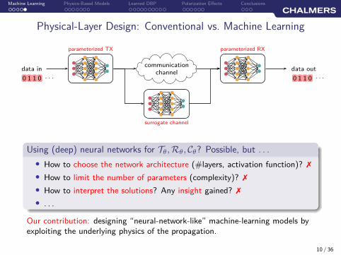
Physical-Layer Design: Conventional vs. Machine Learning
communicationchannel
data in
0 1 1 0 · · ·
parameterized TX
data out
0 1 1 0 · · ·
parameterized RX
surrogate channel
Using (deep) neural networks for Tθ, Rθ, Cθ? Possible, but . . .
• How to choose the network architecture (#layers, activation function)? ✗
• How to limit the number of parameters (complexity)? ✗
• How to interpret the solutions? Any insight gained? ✗
• . . .
Our contribution: designing “neural-network-like” machine-learning models byexploiting the underlying physics of the propagation.
10 / 36
Machine Learning Physics-Based Models Learned DBP Polarization Effects Conclusions
Outline
1. Machine Learning and Neural Networks for Communications
2. Physics-Based Machine Learning for Fiber-Optic Communications
3. Learned Digital Backpropagation
4. Polarization-Dependent Effects
5. Conclusions
11 / 36
Machine Learning Physics-Based Models Learned DBP Polarization Effects Conclusions
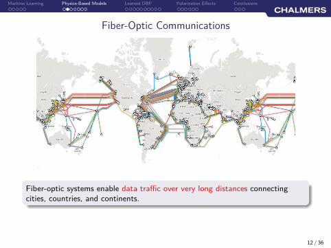
Fiber-Optic Communications
Fiber-optic systems enable data traffic over very long distances connectingcities, countries, and continents.
12 / 36

Machine Learning Physics-Based Models Learned DBP Polarization Effects Conclusions
Fiber-Optic Communications
Fiber-optic systems enable data traffic over very long distances connectingcities, countries, and continents.
• Dispersion: different wavelengths travel at different speeds (linear)• Kerr effect: refractive index changes with signal intensity (nonlinear)
12 / 36
Machine Learning Physics-Based Models Learned DBP Polarization Effects Conclusions
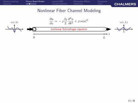
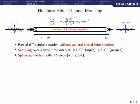
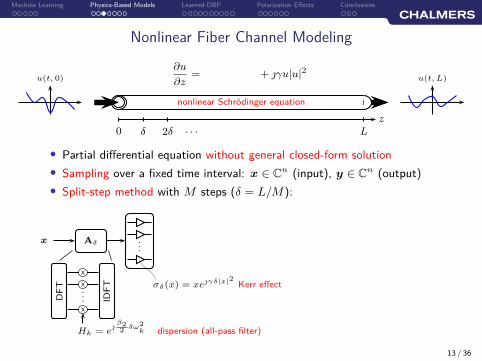
Nonlinear Fiber Channel Modeling
∂u
∂z= −
β2
2
∂2u
∂t2+ γu|u|2
nonlinear Schrödinger equation
z
0 L
u(t, 0) u(t, L)
13 / 36
Machine Learning Physics-Based Models Learned DBP Polarization Effects Conclusions
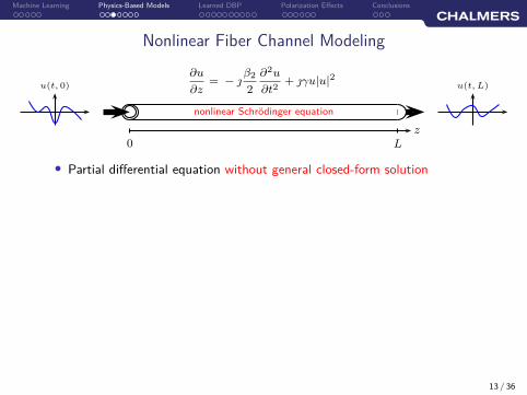
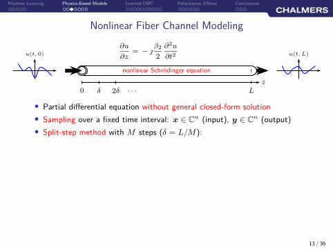
Nonlinear Fiber Channel Modeling
∂u
∂z= −
β2
2
∂2u
∂t2+ γu|u|2
nonlinear Schrödinger equation
z
0 L
u(t, 0) u(t, L)
• Partial differential equation without general closed-form solution
13 / 36
Machine Learning Physics-Based Models Learned DBP Polarization Effects Conclusions
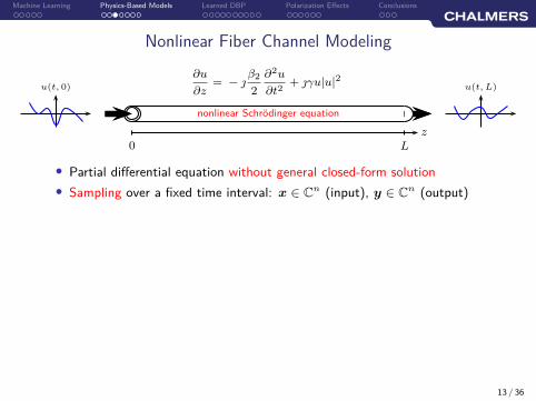
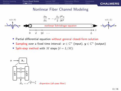
Nonlinear Fiber Channel Modeling
∂u
∂z= −
β2
2
∂2u
∂t2+ γu|u|2
nonlinear Schrödinger equation
z
0 L
u(t, 0) u(t, L)
• Partial differential equation without general closed-form solution
• Sampling over a fixed time interval: x ∈ Cn (input), y ∈ C
n (output)
13 / 36
Machine Learning Physics-Based Models Learned DBP Polarization Effects Conclusions
Nonlinear Fiber Channel Modeling
∂u
∂z= −
β2
2
∂2u
∂t2+ γu|u|2
nonlinear Schrödinger equation
z
0 Lδ 2δ · · ·
u(t, 0) u(t, L)
• Partial differential equation without general closed-form solution
• Sampling over a fixed time interval: x ∈ Cn (input), y ∈ C
n (output)
• Split-step method with M steps (δ = L/M):
13 / 36
Machine Learning Physics-Based Models Learned DBP Polarization Effects Conclusions
Nonlinear Fiber Channel Modeling
∂u
∂z= −
β2
2
∂2u
∂t2
nonlinear Schrödinger equation
z
0 Lδ 2δ · · ·
u(t, 0) u(t, L)
• Partial differential equation without general closed-form solution
• Sampling over a fixed time interval: x ∈ Cn (input), y ∈ C
n (output)
• Split-step method with M steps (δ = L/M):
Aδx
DF
T
... IDF
T
Hk = e
β22
δω2k dispersion (all-pass filter)
13 / 36
Machine Learning Physics-Based Models Learned DBP Polarization Effects Conclusions
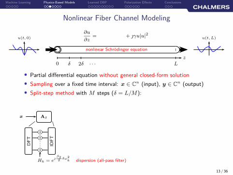
Nonlinear Fiber Channel Modeling
∂u
∂z= + γu|u|2
nonlinear Schrödinger equation
z
0 Lδ 2δ · · ·
u(t, 0) u(t, L)
• Partial differential equation without general closed-form solution
• Sampling over a fixed time interval: x ∈ Cn (input), y ∈ C
n (output)
• Split-step method with M steps (δ = L/M):
Aδx
DF
T
... IDF
T
Hk = e
β22
δω2k dispersion (all-pass filter)
13 / 36
Machine Learning Physics-Based Models Learned DBP Polarization Effects Conclusions
Nonlinear Fiber Channel Modeling
∂u
∂z= + γu|u|2
nonlinear Schrödinger equation
z
0 Lδ 2δ · · ·
u(t, 0) u(t, L)
• Partial differential equation without general closed-form solution
• Sampling over a fixed time interval: x ∈ Cn (input), y ∈ C
n (output)
• Split-step method with M steps (δ = L/M):
Aδx ...
σδ(x) = xeγδ|x|2Kerr effect
DF
T
... IDF
T
Hk = e
β22
δω2k dispersion (all-pass filter)
13 / 36

Machine Learning Physics-Based Models Learned DBP Polarization Effects Conclusions
Nonlinear Fiber Channel Modeling
∂u
∂z= −
β2
2
∂2u
∂t2+ γu|u|2
nonlinear Schrödinger equation
z
0 Lδ 2δ · · ·
u(t, 0) u(t, L)
• Partial differential equation without general closed-form solution
• Sampling over a fixed time interval: x ∈ Cn (input), y ∈ C
n (output)
• Split-step method with M steps (δ = L/M):
Aδx ...
σδ(x) = xeγδ|x|2Kerr effect
DF
T
... IDF
T
Hk = e
β22
δω2k dispersion (all-pass filter)
Aδ ...bbb Aδ ...
≈ y
13 / 36
Machine Learning Physics-Based Models Learned DBP Polarization Effects Conclusions
Deep Learning [LeCun et al., 2015] Deep Q-Learning [Mnih et al., 2015] ResNet [He et al., 2015]
· · ·
[Du and Lowery, 2010] [Nakashima et al., 2017]
14 / 36
Machine Learning Physics-Based Models Learned DBP Polarization Effects Conclusions
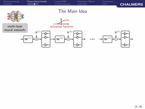
The Main Idea
multi-layerneural network:
W(1)
b(1)
...
activation function
W(2)
b(2)
...bbb
W(ℓ)
b(ℓ)
...
15 / 36

Machine Learning Physics-Based Models Learned DBP Polarization Effects Conclusions
The Main Idea
multi-layerneural network:
W(1)
b(1)
...
activation function
W(2)
b(2)
...bbb
W(ℓ)
b(ℓ)
...
split-stepmethod:
Aδ ...
σ(x) = xeγδ|x|2
Aδ ...
σ(x) = xeγδ|x|2
bbb Aδ ...
σ(x) = xeγδ|x|2
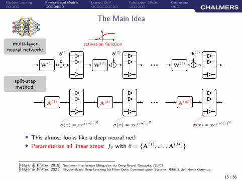
• This almost looks like a deep neural net!
15 / 36
Machine Learning Physics-Based Models Learned DBP Polarization Effects Conclusions
The Main Idea
multi-layerneural network:
W(1)
b(1)
...
activation function
W(2)
b(2)
...bbb
W(ℓ)
b(ℓ)
...
split-stepmethod:
A(1) ...
σ(x) = xeγδ|x|2
A(2) ...
σ(x) = xeγδ|x|2
bbbA
(M) ...
σ(x) = xeγδ|x|2
• This almost looks like a deep neural net!
• Parameterize all linear steps: fθ with θ = {A(1), . . . , A
(M)}
[Häger & Pfister, 2018], Nonlinear Interference Mitigation via Deep Neural Networks, (OFC)[Häger & Pfister, 2021], Physics-Based Deep Learning for Fiber-Optic Communication Systems, IEEE J. Sel. Areas Commun.
15 / 36

Machine Learning Physics-Based Models Learned DBP Polarization Effects Conclusions
The Main Idea
multi-layerneural network:
W(1)
b(1)
...
activation function
W(2)
b(2)
...bbb
W(ℓ)
b(ℓ)
...
split-stepmethod:
A(1) ...
σ(x) = xeγδ|x|2
A(2) ...
σ(x) = xeγδ|x|2
bbbA
(M) ...
σ(x) = xeγδ|x|2
• This almost looks like a deep neural net!
• Parameterize all linear steps: fθ with θ = {A(1), . . . , A
(M)}
• Special cases: step-size optimization, nonlinear operator “placement”, . . .
[Häger & Pfister, 2018], Nonlinear Interference Mitigation via Deep Neural Networks, (OFC)[Häger & Pfister, 2021], Physics-Based Deep Learning for Fiber-Optic Communication Systems, IEEE J. Sel. Areas Commun.
15 / 36
Machine Learning Physics-Based Models Learned DBP Polarization Effects Conclusions
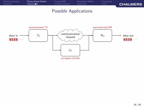
Possible Applications
communicationchannel
data in
0 1 1 0 · · ·
parameterized TX
Tθ data out
0 1 1 0 · · ·
parameterized RX
Rθ
Cθ
surrogate channel
16 / 36
Machine Learning Physics-Based Models Learned DBP Polarization Effects Conclusions
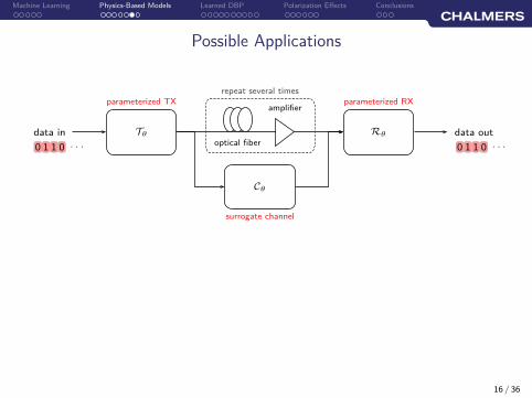
Possible Applications
optical fiber
amplifier
repeat several times
data in
0 1 1 0 · · ·
parameterized TX
Tθ data out
0 1 1 0 · · ·
parameterized RX
Rθ
Cθ
surrogate channel
16 / 36

Machine Learning Physics-Based Models Learned DBP Polarization Effects Conclusions
Possible Applications
optical fiber
amplifier
repeat several times
data in
0 1 1 0 · · ·
parameterized TX
Tθ data out
0 1 1 0 · · ·
parameterized RX
Rθ
Cθ
surrogate channel
• Channel Cθ: fine-tune model based on experimental data, reducesimulation time [Leibrich and Rosenkranz, 2003], [Li et al., 2005]
• Receiver Rθ: nonlinear equalization (focus in this talk)
• Transmitter Tθ: digital pre-distortion [Essiambre and Winzer, 2005],
[Roberts et al., 2006], “split” nonlinearity compensation [Lavery et al., 2016]
16 / 36
Machine Learning Physics-Based Models Learned DBP Polarization Effects Conclusions
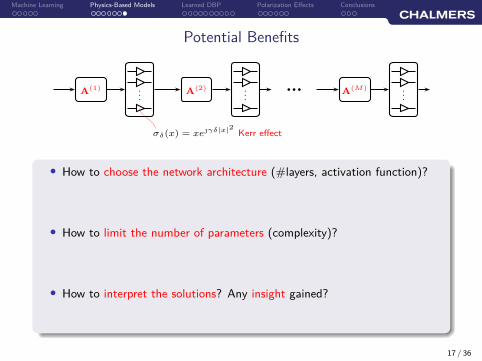
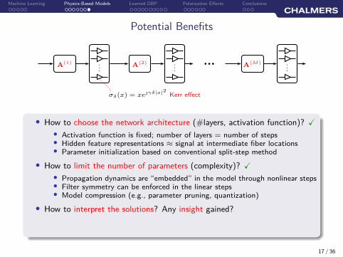
Potential Benefits
A(1) ...
σδ(x) = xeγδ|x|2Kerr effect
A(2) ...
bbbA
(M) ...
• How to choose the network architecture (#layers, activation function)?
• How to limit the number of parameters (complexity)?
• How to interpret the solutions? Any insight gained?
17 / 36
Machine Learning Physics-Based Models Learned DBP Polarization Effects Conclusions
Potential Benefits
A(1) ...
σδ(x) = xeγδ|x|2Kerr effect
A(2) ...
bbbA
(M) ...
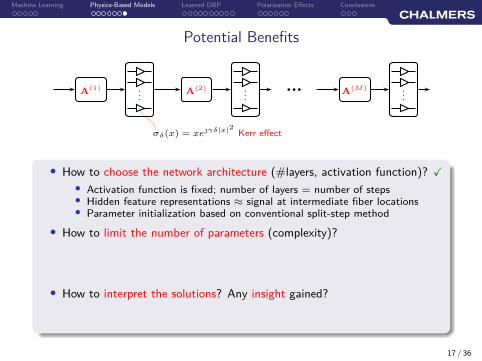
• How to choose the network architecture (#layers, activation function)? X
• Activation function is fixed; number of layers = number of steps• Hidden feature representations ≈ signal at intermediate fiber locations• Parameter initialization based on conventional split-step method
• How to limit the number of parameters (complexity)?
• How to interpret the solutions? Any insight gained?
17 / 36
Machine Learning Physics-Based Models Learned DBP Polarization Effects Conclusions
Potential Benefits
A(1) ...
σδ(x) = xeγδ|x|2Kerr effect
A(2) ...
bbbA
(M) ...
• How to choose the network architecture (#layers, activation function)? X
• Activation function is fixed; number of layers = number of steps• Hidden feature representations ≈ signal at intermediate fiber locations• Parameter initialization based on conventional split-step method
• How to limit the number of parameters (complexity)? X
• Propagation dynamics are “embedded” in the model through nonlinear steps• Filter symmetry can be enforced in the linear steps• Model compression (e.g., parameter pruning, quantization)
• How to interpret the solutions? Any insight gained?
17 / 36

Machine Learning Physics-Based Models Learned DBP Polarization Effects Conclusions
Potential Benefits
A(1) ...
σδ(x) = xeγδ|x|2Kerr effect
A(2) ...
bbbA
(M) ...
• How to choose the network architecture (#layers, activation function)? X
• Activation function is fixed; number of layers = number of steps• Hidden feature representations ≈ signal at intermediate fiber locations• Parameter initialization based on conventional split-step method
• How to limit the number of parameters (complexity)? X
• Propagation dynamics are “embedded” in the model through nonlinear steps• Filter symmetry can be enforced in the linear steps• Model compression (e.g., parameter pruning, quantization)
• How to interpret the solutions? Any insight gained? X
• Learned parameter configurations are interpretable• Satisfactory explanations for benefits over previous handcrafted solutions
17 / 36
Machine Learning Physics-Based Models Learned DBP Polarization Effects Conclusions
Outline
1. Machine Learning and Neural Networks for Communications
2. Physics-Based Machine Learning for Fiber-Optic Communications
3. Learned Digital Backpropagation
4. Polarization-Dependent Effects
5. Conclusions
18 / 36
Machine Learning Physics-Based Models Learned DBP Polarization Effects Conclusions
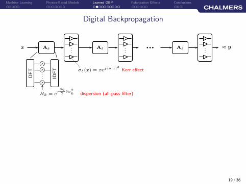
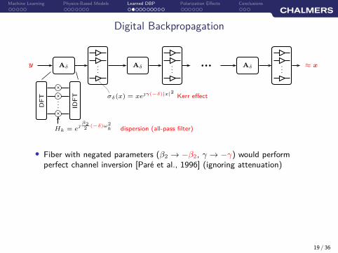
Digital Backpropagation
Aδx ...
σδ(x) = xeγδ|x|2Kerr effect
DF
T
... IDF
T
Hk = e
β22
δω2k dispersion (all-pass filter)
Aδ ...bbb Aδ ...
≈ y
19 / 36
Machine Learning Physics-Based Models Learned DBP Polarization Effects Conclusions
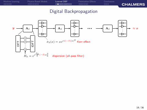
Digital Backpropagation
Aδy ...
σδ(x) = xeγ(−δ)|x|2Kerr effect
DF
T
... IDF
T
Hk = e
β22
(−δ)ω2k dispersion (all-pass filter)
Aδ ...bbb Aδ ...
≈ x
19 / 36
Machine Learning Physics-Based Models Learned DBP Polarization Effects Conclusions
Digital Backpropagation
Aδy ...
σδ(x) = xeγ(−δ)|x|2Kerr effect
DF
T
... IDF
T
Hk = e
β22
(−δ)ω2k dispersion (all-pass filter)
Aδ ...bbb Aδ ...
≈ x
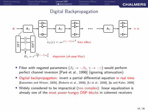
• Fiber with negated parameters (β2 → −β2, γ → −γ) would performperfect channel inversion [Paré et al., 1996] (ignoring attenuation)
19 / 36

Machine Learning Physics-Based Models Learned DBP Polarization Effects Conclusions
Digital Backpropagation
Aδy ...
σδ(x) = xeγ(−δ)|x|2Kerr effect
DF
T
... IDF
T
Hk = e
β22
(−δ)ω2k dispersion (all-pass filter)
Aδ ...bbb Aδ ...
≈ x
• Fiber with negated parameters (β2 → −β2, γ → −γ) would performperfect channel inversion [Paré et al., 1996] (ignoring attenuation)
• Digital backpropagation: invert a partial differential equation in real time[Essiambre and Winzer, 2005], [Roberts et al., 2006], [Li et al., 2008], [Ip and Kahn, 2008]
19 / 36
Machine Learning Physics-Based Models Learned DBP Polarization Effects Conclusions
Digital Backpropagation
Aδy ...
σδ(x) = xeγ(−δ)|x|2Kerr effect
DF
T
... IDF
T
Hk = e
β22
(−δ)ω2k dispersion (all-pass filter)
Aδ ...bbb Aδ ...
≈ x
• Fiber with negated parameters (β2 → −β2, γ → −γ) would performperfect channel inversion [Paré et al., 1996] (ignoring attenuation)
• Digital backpropagation: invert a partial differential equation in real time[Essiambre and Winzer, 2005], [Roberts et al., 2006], [Li et al., 2008], [Ip and Kahn, 2008]
• Widely considered to be impractical (too complex): linear equalization isalready one of the most power-hungry DSP blocks in coherent receivers
19 / 36

Machine Learning Physics-Based Models Learned DBP Polarization Effects Conclusions
Real-Time Digital Backpropagation
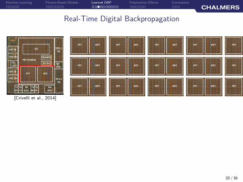
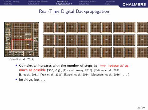
[Crivelli et al., 2014]
20 / 36
Machine Learning Physics-Based Models Learned DBP Polarization Effects Conclusions
Real-Time Digital Backpropagation
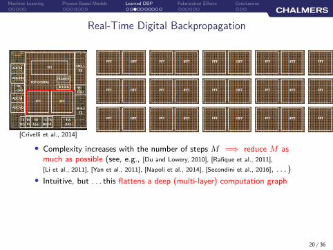
[Crivelli et al., 2014]
20 / 36
Machine Learning Physics-Based Models Learned DBP Polarization Effects Conclusions
Real-Time Digital Backpropagation
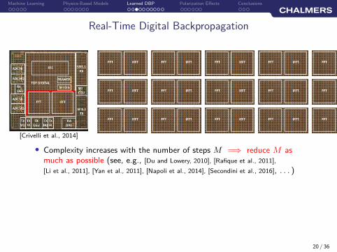
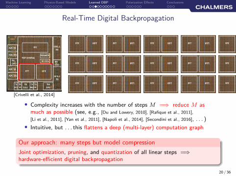
[Crivelli et al., 2014]
• Complexity increases with the number of steps M =⇒ reduce M asmuch as possible (see, e.g., [Du and Lowery, 2010], [Rafique et al., 2011],
[Li et al., 2011], [Yan et al., 2011], [Napoli et al., 2014], [Secondini et al., 2016], . . . )
20 / 36
Machine Learning Physics-Based Models Learned DBP Polarization Effects Conclusions
Real-Time Digital Backpropagation
[Crivelli et al., 2014]
• Complexity increases with the number of steps M =⇒ reduce M asmuch as possible (see, e.g., [Du and Lowery, 2010], [Rafique et al., 2011],
[Li et al., 2011], [Yan et al., 2011], [Napoli et al., 2014], [Secondini et al., 2016], . . . )
• Intuitive, but . . .
20 / 36
Machine Learning Physics-Based Models Learned DBP Polarization Effects Conclusions
Real-Time Digital Backpropagation
[Crivelli et al., 2014]
• Complexity increases with the number of steps M =⇒ reduce M asmuch as possible (see, e.g., [Du and Lowery, 2010], [Rafique et al., 2011],
[Li et al., 2011], [Yan et al., 2011], [Napoli et al., 2014], [Secondini et al., 2016], . . . )
• Intuitive, but . . . this flattens a deep (multi-layer) computation graph
Our approach: many steps but model compression
Joint optimization, pruning, and quantization of all linear steps =⇒hardware-efficient digital backpropagation
20 / 36
Machine Learning Physics-Based Models Learned DBP Polarization Effects Conclusions
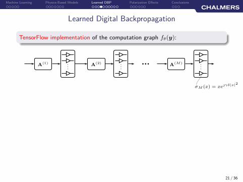
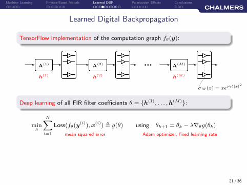
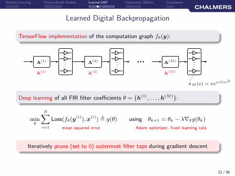
Learned Digital Backpropagation
TensorFlow implementation of the computation graph fθ(y):
A(1) ...
A(2) ...
bbbA
(M) ...
σM (x) = xeγδ|x|2
21 / 36

Machine Learning Physics-Based Models Learned DBP Polarization Effects Conclusions
Learned Digital Backpropagation
TensorFlow implementation of the computation graph fθ(y):
h(1) h(2) h(M)
A(1) ...
A(2) ...
bbbA
(M) ...
σM (x) = xeγδ|x|2
h(i)0
h(i)1
h(i)2
h(i)3
h(i)4
h(i)5
h(i)6
h(i)7
h(i)8
h(i)9
h(i)1
h(i)0
h(i)1
h(i)2
h(i)3
h(i)4
h(i)5
h(i)6
h(i)7
h(i)8
h(i)2
h(i)1
h(i)0
h(i)1
h(i)2
h(i)3
h(i)4
h(i)5
h(i)6
h(i)7
h(i)3
h(i)2
h(i)1
h(i)0
h(i)1
h(i)2
h(i)3
h(i)4
h(i)5
h(i)6
h(i)4
h(i)3
h(i)2
h(i)1
h(i)0
h(i)1
h(i)2
h(i)3
h(i)4
h(i)5
h(i)5
h(i)4
h(i)3
h(i)2
h(i)1
h(i)0
h(i)1
h(i)2
h(i)3
h(i)4
h(i)6
h(i)5
h(i)4
h(i)3
h(i)2
h(i)1
h(i)0
h(i)1
h(i)2
h(i)3
h(i)7
h(i)6
h(i)5
h(i)4
h(i)3
h(i)2
h(i)1
h(i)0
h(i)1
h(i)2
h(i)8
h(i)7
h(i)6
h(i)5
h(i)4
h(i)3
h(i)2
h(i)1
h(i)0
h(i)1
h(i)9
h(i)8
h(i)7
h(i)6
h(i)5
h(i)4
h(i)3
h(i)2
h(i)1
h(i)0
· · ·
...
. . .
0
0
0
0
0
0
0
0
0
0
0
0
0
0
0
0
0
0
0
0
0
0
0
0
0
0
0
0
0
0
finite impulse response (FIR) filtercomplex & symmetric coefficients
h(i)2
b D
h(i)1
b D
h(i)0
b D
h(i)1
b D
h(i)2
21 / 36
Machine Learning Physics-Based Models Learned DBP Polarization Effects Conclusions
Learned Digital Backpropagation
TensorFlow implementation of the computation graph fθ(y):
h(1) h(2) h(M)
A(1) ...
A(2) ...
bbbA
(M) ...
σM (x) = xeγδ|x|2
mean squared error Adam optimizer, fixed learning rate
Deep learning of all FIR filter coefficients θ = {h(1), . . . , h(M)}:
minθ
N∑
i=1
Loss(fθ(y(i)), x(i)) , g(θ) using θk+1 = θk − λ∇θg(θk)
Iteratively prune (set to 0) outermost filter taps during gradient descent
21 / 36
Machine Learning Physics-Based Models Learned DBP Polarization Effects Conclusions
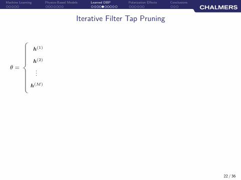
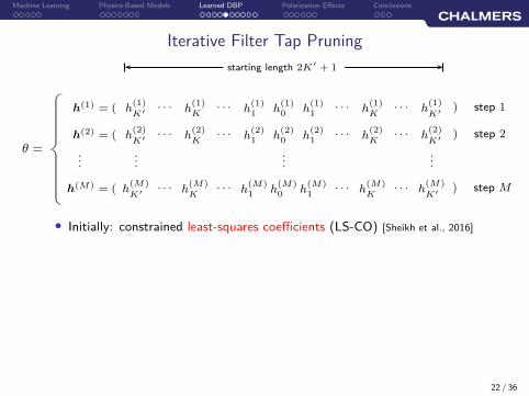
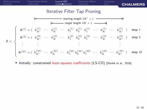
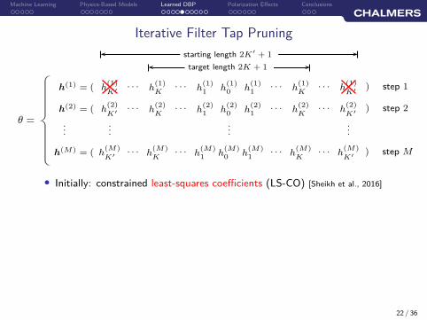
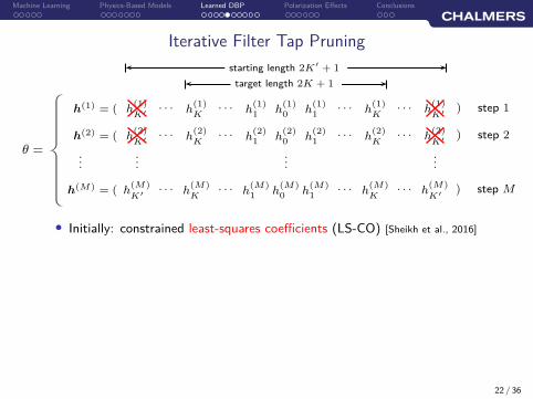
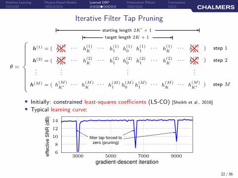
Iterative Filter Tap Pruning
θ =
h(1)
h(2)
...
h(M)
22 / 36
Machine Learning Physics-Based Models Learned DBP Polarization Effects Conclusions
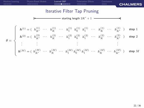
Iterative Filter Tap Pruning
θ =
starting length 2K′ + 1
h(1) = ( h(1)1
· · ·h(1)K
· · ·h(1)
K′ h(1)0 h
(1)1
· · · h(1)K
· · · h(1)
K′ ) step 1
h(2) = ( h(2)1
· · ·h(2)K
· · ·h(2)
K′ h(2)0 h
(2)1
· · · h(2)K
· · · h(2)
K′ ) step 2
......
......
h(M) = ( h(M)1
· · ·h(M)K
· · ·h(M)
K′ h(M)0 h
(M)1
· · · h(M)K
· · · h(M)
K′ ) step M
22 / 36
Machine Learning Physics-Based Models Learned DBP Polarization Effects Conclusions
Iterative Filter Tap Pruning
θ =
starting length 2K′ + 1
h(1) = ( h(1)1
· · ·h(1)K
· · ·h(1)
K′ h(1)0 h
(1)1
· · · h(1)K
· · · h(1)
K′ ) step 1
h(2) = ( h(2)1
· · ·h(2)K
· · ·h(2)
K′ h(2)0 h
(2)1
· · · h(2)K
· · · h(2)
K′ ) step 2
......
......
h(M) = ( h(M)1
· · ·h(M)K
· · ·h(M)
K′ h(M)0 h
(M)1
· · · h(M)K
· · · h(M)
K′ ) step M
• Initially: constrained least-squares coefficients (LS-CO) [Sheikh et al., 2016]
22 / 36
Machine Learning Physics-Based Models Learned DBP Polarization Effects Conclusions
Iterative Filter Tap Pruning
θ =
starting length 2K′ + 1
target length 2K + 1
h(1) = ( h(1)1
· · ·h(1)K
· · ·h(1)
K′ h(1)0 h
(1)1
· · · h(1)K
· · · h(1)
K′ ) step 1
h(2) = ( h(2)1
· · ·h(2)K
· · ·h(2)
K′ h(2)0 h
(2)1
· · · h(2)K
· · · h(2)
K′ ) step 2
......
......
h(M) = ( h(M)1
· · ·h(M)K
· · ·h(M)
K′ h(M)0 h
(M)1
· · · h(M)K
· · · h(M)
K′ ) step M
• Initially: constrained least-squares coefficients (LS-CO) [Sheikh et al., 2016]
• Typical learning curve:
6
8
10
12
14
gradient-descent iteration
effective
SN
R(d
B)
3000 5000 7000 9000
filter tap forced tozero (pruning)
22 / 36
Machine Learning Physics-Based Models Learned DBP Polarization Effects Conclusions
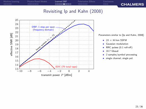
Revisiting Ip and Kahn (2008)
−10 −8 −6 −4 −2 0 2 413
14
15
16
17
18
19
20
21
22
23
24
25
transmit power P [dBm]
effec
tive
SN
R[d
B]
linea
r syst
em(γ
=0)
EDC (75 total taps)
DBP, 1 step per span(frequency-domain)
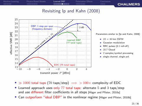
Parameters similar to [Ip and Kahn, 2008]:
• 25 × 80 km SSFM
• Gaussian modulation
• RRC pulses (0.1 roll-off)
• 10.7 Gbaud
• 2 samples/symbol processing
• single channel, single pol.
23 / 36
Machine Learning Physics-Based Models Learned DBP Polarization Effects Conclusions
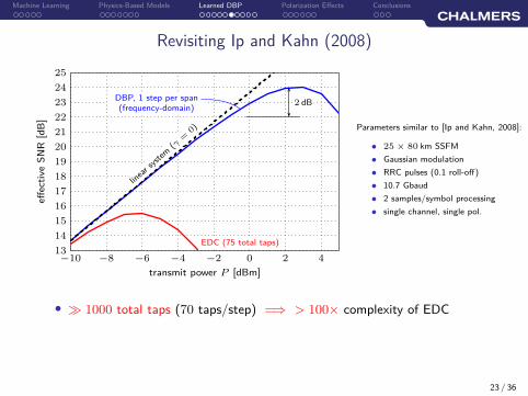
Revisiting Ip and Kahn (2008)
−10 −8 −6 −4 −2 0 2 413
14
15
16
17
18
19
20
21
22
23
24
25
transmit power P [dBm]
effec
tive
SN
R[d
B]
linea
r syst
em(γ
=0)
EDC (75 total taps)
DBP, 1 step per span(frequency-domain)
2 dB
Parameters similar to [Ip and Kahn, 2008]:
• 25 × 80 km SSFM
• Gaussian modulation
• RRC pulses (0.1 roll-off)
• 10.7 Gbaud
• 2 samples/symbol processing
• single channel, single pol.
• ≫ 1000 total taps (70 taps/step) =⇒ > 100× complexity of EDC
23 / 36
Machine Learning Physics-Based Models Learned DBP Polarization Effects Conclusions
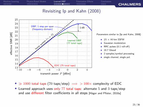
Revisiting Ip and Kahn (2008)
−10 −8 −6 −4 −2 0 2 413
14
15
16
17
18
19
20
21
22
23
24
25
transmit power P [dBm]
effec
tive
SN
R[d
B]
uTuT uT uT
uT
linea
r syst
em(γ
=0)
EDC (75 total taps)
Learned DBP(77 total taps)
DBP, 1 step per span(frequency-domain)
2 dB
Parameters similar to [Ip and Kahn, 2008]:
• 25 × 80 km SSFM
• Gaussian modulation
• RRC pulses (0.1 roll-off)
• 10.7 Gbaud
• 2 samples/symbol processing
• single channel, single pol.
• ≫ 1000 total taps (70 taps/step) =⇒ > 100× complexity of EDC
• Learned approach uses only 77 total taps: alternate 5 and 3 taps/stepand use different filter coefficients in all steps [Häger and Pfister, 2018a]
23 / 36
Machine Learning Physics-Based Models Learned DBP Polarization Effects Conclusions
Revisiting Ip and Kahn (2008)
−10 −8 −6 −4 −2 0 2 413
14
15
16
17
18
19
20
21
22
23
24
25
transmit power P [dBm]
effec
tive
SN
R[d
B]
uTuT uT uT
uT
linea
r syst
em(γ
=0)
EDC (75 total taps)
Learned DBP(77 total taps)
DBP, 1 step per span(frequency-domain)
2 dB
Parameters similar to [Ip and Kahn, 2008]:
• 25 × 80 km SSFM
• Gaussian modulation
• RRC pulses (0.1 roll-off)
• 10.7 Gbaud
• 2 samples/symbol processing
• single channel, single pol.
• ≫ 1000 total taps (70 taps/step) =⇒ > 100× complexity of EDC
• Learned approach uses only 77 total taps: alternate 5 and 3 taps/stepand use different filter coefficients in all steps [Häger and Pfister, 2018a]
• Can outperform “ideal DBP” in the nonlinear regime [Häger and Pfister, 2018b]
23 / 36
Machine Learning Physics-Based Models Learned DBP Polarization Effects Conclusions
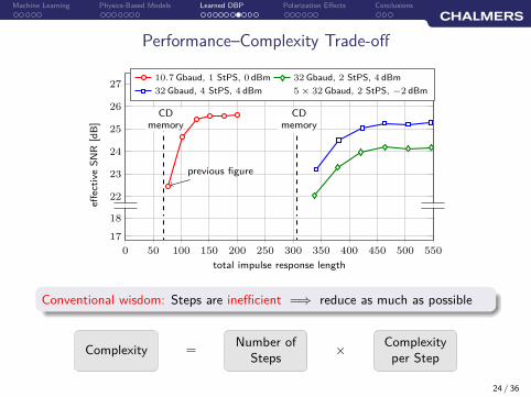
Performance–Complexity Trade-off
22
23
24
25
26
27
CDmemory
CDmemory
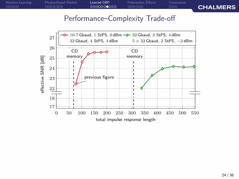
previous figure
effec
tive
SN
R[d
B]
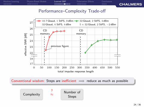
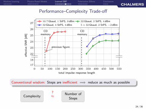
10.7 Gbaud, 1 StPS, 0 dBm 32 Gbaud, 2 StPS, 4 dBm
32 Gbaud, 4 StPS, 4 dBm 5 × 32 Gbaud, 2 StPS, −2 dBm
0 50 100 150 200 250 300 350 400 450 500 550
17
18
total impulse response length
24 / 36
Machine Learning Physics-Based Models Learned DBP Polarization Effects Conclusions
Performance–Complexity Trade-off
22
23
24
25
26
27
CDmemory
CDmemory
previous figure
effec
tive
SN
R[d
B]
10.7 Gbaud, 1 StPS, 0 dBm 32 Gbaud, 2 StPS, 4 dBm
32 Gbaud, 4 StPS, 4 dBm 5 × 32 Gbaud, 2 StPS, −2 dBm
0 50 100 150 200 250 300 350 400 450 500 550
17
18
total impulse response length
Conventional wisdom: Steps are inefficient =⇒ reduce as much as possible
Complexity ≈? Number of
Steps
24 / 36
Machine Learning Physics-Based Models Learned DBP Polarization Effects Conclusions
Performance–Complexity Trade-off
22
23
24
25
26
27
CDmemory
CDmemory
previous figure
effec
tive
SN
R[d
B]
10.7 Gbaud, 1 StPS, 0 dBm 32 Gbaud, 2 StPS, 4 dBm
32 Gbaud, 4 StPS, 4 dBm 5 × 32 Gbaud, 2 StPS, −2 dBm
0 50 100 150 200 250 300 350 400 450 500 550
17
18
total impulse response length
Conventional wisdom: Steps are inefficient =⇒ reduce as much as possible
ComplexityNumber of
Steps= ×
Complexityper Step
24 / 36
Machine Learning Physics-Based Models Learned DBP Polarization Effects Conclusions
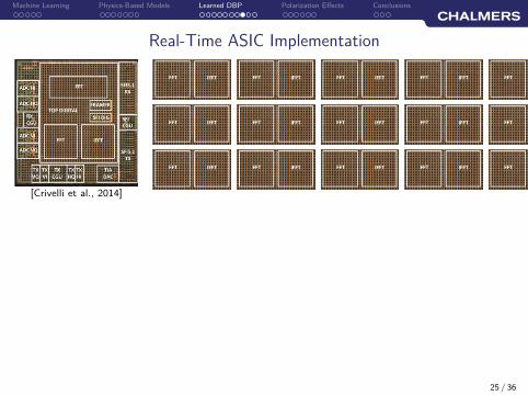
Real-Time ASIC Implementation
[Crivelli et al., 2014]
25 / 36
Machine Learning Physics-Based Models Learned DBP Polarization Effects Conclusions
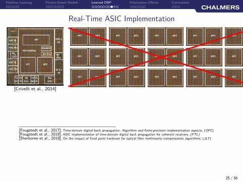
Real-Time ASIC Implementation
[Crivelli et al., 2014]
[Fougstedt et al., 2017], Time-domain digital back propagation: Algorithm and finite-precision implementation aspects, (OFC)[Fougstedt et al., 2018], ASIC implementation of time-domain digital back propagation for coherent receivers, (PTL)[Sherborne et al., 2018], On the impact of fixed point hardware for optical fiber nonlinearity compensation algorithms, (JLT)
25 / 36
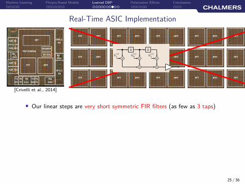
Machine Learning Physics-Based Models Learned DBP Polarization Effects Conclusions
Real-Time ASIC Implementation
[Crivelli et al., 2014]
h(i)1
b D
h(i)0
b D
h(i)1
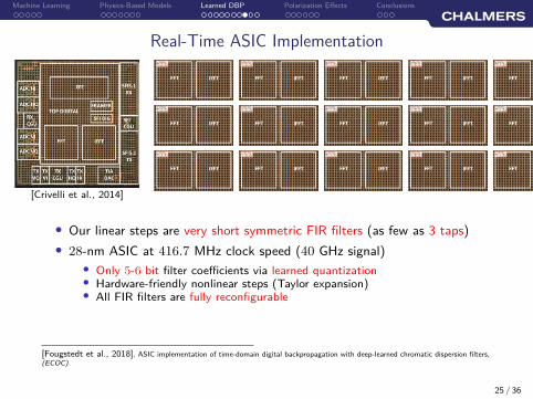
• Our linear steps are very short symmetric FIR filters (as few as 3 taps)
25 / 36
Machine Learning Physics-Based Models Learned DBP Polarization Effects Conclusions
Real-Time ASIC Implementation
[Crivelli et al., 2014]
h(i)1
b D
h(i)0
b D
h(i)1 h
(i)1
b D
h(i)0
b D
h(i)1 h
(i)1
b D
h(i)0
b D
h(i)1 h
(i)1
b D
h(i)0
b D
h(i)1 h
(i)1
b D
h(i)0
b D
h(i)1
h(i)1
b D
h(i)0
b D
h(i)1 h
(i)1
b D
h(i)0
b D
h(i)1 h
(i)1
b D
h(i)0
b D
h(i)1 h
(i)1
b D
h(i)0
b D
h(i)1 h
(i)1
b D
h(i)0
b D
h(i)1
h(i)1
b D
h(i)0
b D
h(i)1 h
(i)1
b D
h(i)0
b D
h(i)1 h
(i)1
b D
h(i)0
b D
h(i)1 h
(i)1
b D
h(i)0
b D
h(i)1 h
(i)1
b D
h(i)0
b D
h(i)1
• Our linear steps are very short symmetric FIR filters (as few as 3 taps)
• 28-nm ASIC at 416.7 MHz clock speed (40 GHz signal)
• Only 5-6 bit filter coefficients via learned quantization• Hardware-friendly nonlinear steps (Taylor expansion)• All FIR filters are fully reconfigurable
[Fougstedt et al., 2018], ASIC implementation of time-domain digital backpropagation with deep-learned chromatic dispersion filters,(ECOC)
25 / 36
Machine Learning Physics-Based Models Learned DBP Polarization Effects Conclusions
Real-Time ASIC Implementation
[Crivelli et al., 2014]
h(i)1
b D
h(i)0
b D
h(i)1 h
(i)1
b D
h(i)0
b D
h(i)1 h
(i)1
b D
h(i)0
b D
h(i)1 h
(i)1
b D
h(i)0
b D
h(i)1 h
(i)1
b D
h(i)0
b D
h(i)1
h(i)1
b D
h(i)0
b D
h(i)1 h
(i)1
b D
h(i)0
b D
h(i)1 h
(i)1
b D
h(i)0
b D
h(i)1 h
(i)1
b D
h(i)0
b D
h(i)1 h
(i)1
b D
h(i)0
b D
h(i)1
h(i)1
b D
h(i)0
b D
h(i)1 h
(i)1
b D
h(i)0
b D
h(i)1 h
(i)1
b D
h(i)0
b D
h(i)1 h
(i)1
b D
h(i)0
b D
h(i)1 h
(i)1
b D
h(i)0
b D
h(i)1
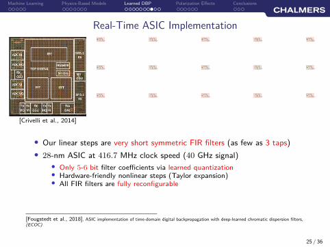
• Our linear steps are very short symmetric FIR filters (as few as 3 taps)
• 28-nm ASIC at 416.7 MHz clock speed (40 GHz signal)
• Only 5-6 bit filter coefficients via learned quantization• Hardware-friendly nonlinear steps (Taylor expansion)• All FIR filters are fully reconfigurable
[Fougstedt et al., 2018], ASIC implementation of time-domain digital backpropagation with deep-learned chromatic dispersion filters,(ECOC)
25 / 36
Machine Learning Physics-Based Models Learned DBP Polarization Effects Conclusions
Real-Time ASIC Implementation
[Crivelli et al., 2014]
h(i)1
b D
h(i)0
b D
h(i)1 h
(i)1
b D
h(i)0
b D
h(i)1 h
(i)1
b D
h(i)0
b D
h(i)1 h
(i)1
b D
h(i)0
b D
h(i)1 h
(i)1
b D
h(i)0
b D
h(i)1 h
(i)1
b D
h(i)0
b D
h(i)1
h(i)1
b D
h(i)0
b D
h(i)1 h
(i)1
b D
h(i)0
b D
h(i)1 h
(i)1
b D
h(i)0
b D
h(i)1 h
(i)1
b D
h(i)0
b D
h(i)1 h
(i)1
b D
h(i)0
b D
h(i)1 h
(i)1
b D
h(i)0
b D
h(i)1
h(i)1
b D
h(i)0
b D
h(i)1 h
(i)1
b D
h(i)0
b D
h(i)1 h
(i)1
b D
h(i)0
b D
h(i)1 h
(i)1
b D
h(i)0
b D
h(i)1 h
(i)1
b D
h(i)0
b D
h(i)1 h
(i)1
b D
h(i)0
b D
h(i)1
h(i)1
b D
h(i)0
b D
h(i)1 h
(i)1
b D
h(i)0
b D
h(i)1 h
(i)1
b D
h(i)0
b D
h(i)1 h
(i)1
b D
h(i)0
b D
h(i)1 h
(i)1
b D
h(i)0
b D
h(i)1 h
(i)1
b D
h(i)0
b D
h(i)1
h(i)1
b D
h(i)0
b D
h(i)1 h
(i)1
b D
h(i)0
b D
h(i)1 h
(i)1
b D
h(i)0
b D
h(i)1 h
(i)1
b D
h(i)0
b D
h(i)1 h
(i)1
b D
h(i)0
b D
h(i)1 h
(i)1
b D
h(i)0
b D
h(i)1
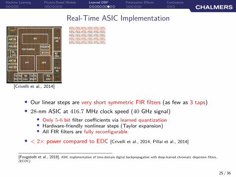
• Our linear steps are very short symmetric FIR filters (as few as 3 taps)
• 28-nm ASIC at 416.7 MHz clock speed (40 GHz signal)
• Only 5-6 bit filter coefficients via learned quantization• Hardware-friendly nonlinear steps (Taylor expansion)• All FIR filters are fully reconfigurable
• < 2× power compared to EDC [Crivelli et al., 2014, Pillai et al., 2014]
[Fougstedt et al., 2018], ASIC implementation of time-domain digital backpropagation with deep-learned chromatic dispersion filters,(ECOC)
25 / 36
Machine Learning Physics-Based Models Learned DBP Polarization Effects Conclusions
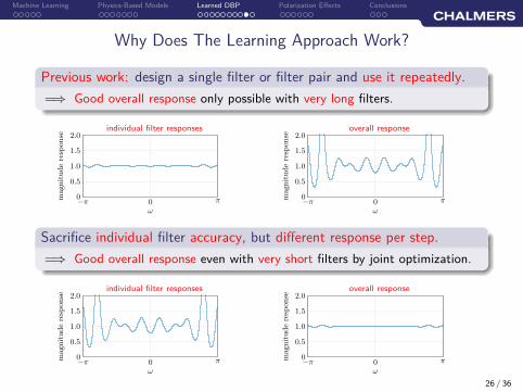
Why Does The Learning Approach Work?
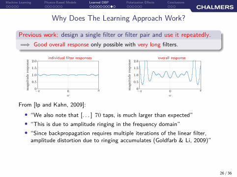
Previous work: design a single filter or filter pair and use it repeatedly.
=⇒ Good overall response only possible with very long filters.
individual filter responses
0
0.5
1.0
1.5
2.0
ω
magnituderesp
onse
0 π−π
overall response
0
0.5
1.0
1.5
2.0
ω
magnituderesp
onse
0 π−π
From [Ip and Kahn, 2009]:
• “We also note that [. . . ] 70 taps, is much larger than expected”
• “This is due to amplitude ringing in the frequency domain”
• “Since backpropagation requires multiple iterations of the linear filter,amplitude distortion due to ringing accumulates (Goldfarb & Li, 2009)”
26 / 36

Machine Learning Physics-Based Models Learned DBP Polarization Effects Conclusions
Why Does The Learning Approach Work?
Previous work: design a single filter or filter pair and use it repeatedly.
=⇒ Good overall response only possible with very long filters.
individual filter responses
0
0.5
1.0
1.5
2.0
ω
magnituderesp
onse
0 π−π
overall response
0
0.5
1.0
1.5
2.0
ω
magnituderesp
onse
0 π−π
From [Ip and Kahn, 2009]:
• “We also note that [. . . ] 70 taps, is much larger than expected”
• “This is due to amplitude ringing in the frequency domain”
• “Since backpropagation requires multiple iterations of the linear filter,amplitude distortion due to ringing accumulates (Goldfarb & Li, 2009)”
The learning approach uncovered that there is no such requirement![Lian, Häger, Pfister, 2018], What can machine learning teach us about communications? (ITW)
26 / 36
Machine Learning Physics-Based Models Learned DBP Polarization Effects Conclusions
Why Does The Learning Approach Work?
Previous work: design a single filter or filter pair and use it repeatedly.
=⇒ Good overall response only possible with very long filters.
individual filter responses
0
0.5
1.0
1.5
2.0
ω
magnituderesp
onse
0 π−π
overall response
0
0.5
1.0
1.5
2.0
ω
magnituderesp
onse
0 π−π
Sacrifice individual filter accuracy, but different response per step.
=⇒ Good overall response even with very short filters by joint optimization.
individual filter responses
0
0.5
1.0
1.5
2.0
ω
magnituderesp
onse
0 π−π
overall response
0
0.5
1.0
1.5
2.0
ω
magnituderesp
onse
0 π−π
26 / 36
Machine Learning Physics-Based Models Learned DBP Polarization Effects Conclusions
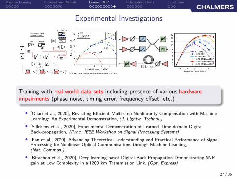
Experimental Investigations
Training with real-world data sets including presence of various hardwareimpairments (phase noise, timing error, frequency offset, etc.)
• [Oliari et al., 2020], Revisiting Efficient Multi-step Nonlinearity Compensation with MachineLearning: An Experimental Demonstration, (J. Lightw. Technol.)
• [Sillekens et al., 2020], Experimental Demonstration of Learned Time-domain DigitalBack-propagation, (Proc. IEEE Workshop on Signal Processing Systems)
• [Fan et al., 2020], Advancing Theoretical Understanding and Practical Performance of SignalProcessing for Nonlinear Optical Communications through Machine Learning,(Nat. Commun.)
• [Bitachon et al., 2020], Deep learning based Digital Back Propagation Demonstrating SNRgain at Low Complexity in a 1200 km Transmission Link, (Opt. Express)
27 / 36

Machine Learning Physics-Based Models Learned DBP Polarization Effects Conclusions
Outline
1. Machine Learning and Neural Networks for Communications
2. Physics-Based Machine Learning for Fiber-Optic Communications
3. Learned Digital Backpropagation
4. Polarization-Dependent Effects
5. Conclusions
28 / 36

Machine Learning Physics-Based Models Learned DBP Polarization Effects Conclusions
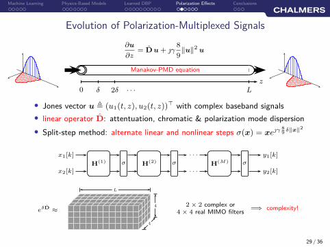
Evolution of Polarization-Multiplexed Signals
∂u
∂z= D̂ u + γ
8
9‖u‖2 u
Manakov-PMD equation
z
0 Lδ 2δ · · ·
• Jones vector u , (u1(t, z), u2(t, z))⊤ with complex baseband signals
• linear operator D̂: attentuation, chromatic & polarization mode dispersion
29 / 36
Machine Learning Physics-Based Models Learned DBP Polarization Effects Conclusions
Evolution of Polarization-Multiplexed Signals
∂u
∂z= D̂ u + γ
8
9‖u‖2 u
Manakov-PMD equation
z
0 Lδ 2δ · · ·
• Jones vector u , (u1(t, z), u2(t, z))⊤ with complex baseband signals
• linear operator D̂: attentuation, chromatic & polarization mode dispersion
• Split-step method: alternate linear and nonlinear steps σ(x) = xeγ 89
δ‖x‖2
x1[k]
x2[k]H
(1) σ H(2) σ
· · ·
· · ·
H(M) σ
y1[k]
y2[k]
eδD̂≈
4
4
L
2 × 2 complex or4 × 4 real MIMO filters
=⇒ complexity!
29 / 36
Machine Learning Physics-Based Models Learned DBP Polarization Effects Conclusions
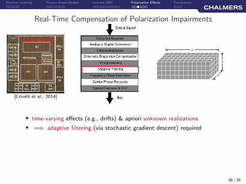
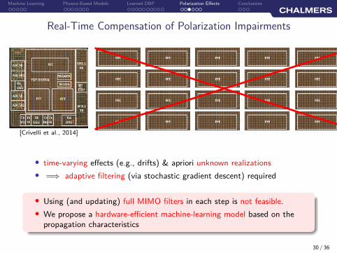
Real-Time Compensation of Polarization Impairments
[Crivelli et al., 2014]
4
4
L
• time-varying effects (e.g., drifts) & apriori unknown realizations
• =⇒ adaptive filtering (via stochastic gradient descent) required
30 / 36
Machine Learning Physics-Based Models Learned DBP Polarization Effects Conclusions
Real-Time Compensation of Polarization Impairments
[Crivelli et al., 2014]
• time-varying effects (e.g., drifts) & apriori unknown realizations
• =⇒ adaptive filtering (via stochastic gradient descent) required
• Using (and updating) full MIMO filters in each step is not feasible.
• We propose a hardware-efficient machine-learning model based on thepropagation characteristics
30 / 36
Machine Learning Physics-Based Models Learned DBP Polarization Effects Conclusions
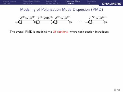
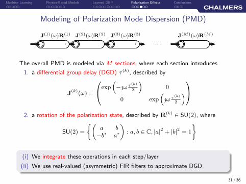
Modeling of Polarization Mode Dispersion (PMD)
J(M)(ω)R(M)
· · ·
J(3)(ω)R(3)
J(2)(ω)R(2)
J(1)(ω)R(1)
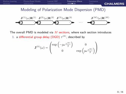
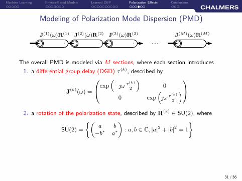
The overall PMD is modeled via M sections, where each section introduces
31 / 36
Machine Learning Physics-Based Models Learned DBP Polarization Effects Conclusions
Modeling of Polarization Mode Dispersion (PMD)
J(M)(ω)R(M)
· · ·
J(3)(ω)R(3)
J(2)(ω)R(2)
J(1)(ω)R(1)
The overall PMD is modeled via M sections, where each section introduces
1. a differential group delay (DGD) τ (k), described by
J(k)(ω) =
exp(
−ω τ(k)
2
)
0
0 exp(
ω τ(k)
2
)
2. a rotation of the polarization state, described by R(k) ∈ SU(2), where
SU(2) =
{(
a b−b∗ a∗
)
: a, b ∈ C, |a|2 + |b|2 = 1
}
(i) We integrate these operations in each step/layer
(ii) We use real-valued (asymmetric) FIR filters to approximate DGD
31 / 36
Machine Learning Physics-Based Models Learned DBP Polarization Effects Conclusions
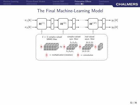
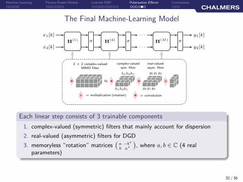
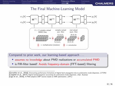
The Final Machine-Learning Model
∗ ≈
2 × 2 complex-valuedMIMO filter
real-valuedasym. filter
complex-valuedsym. filter
× = multiplication (rotation) ∗ = convolution
h1h0h1
h1h0h1
∗ ∗
g2 g1 g0
g0 g1 g2
∗ ×
x1[k]
x2[k]H
(1) σ H(2) σ
· · ·
· · ·
H(M) σ
y1[k]
y2[k]
32 / 36
Machine Learning Physics-Based Models Learned DBP Polarization Effects Conclusions
The Final Machine-Learning Model
∗ ≈
2 × 2 complex-valuedMIMO filter
real-valuedasym. filter
complex-valuedsym. filter
× = multiplication (rotation) ∗ = convolution
h1h0h1
h1h0h1
∗ ∗
g2 g1 g0
g0 g1 g2
∗ ×
x1[k]
x2[k]H
(1) σ H(2) σ
· · ·
· · ·
H(M) σ
y1[k]
y2[k]
Each linear step consists of 3 trainable components
1. complex-valued (symmetric) filters that mainly account for dispersion
2. real-valued (asymmetric) filters for DGD
3. memoryless “rotation” matrices(
a −b∗
b a∗
)
, where a, b ∈ C (4 realparameters)
32 / 36
Machine Learning Physics-Based Models Learned DBP Polarization Effects Conclusions
The Final Machine-Learning Model
∗ ≈
2 × 2 complex-valuedMIMO filter
real-valuedasym. filter
complex-valuedsym. filter
× = multiplication (rotation) ∗ = convolution
h1h0h1
h1h0h1
∗ ∗
g2 g1 g0
g0 g1 g2
∗ ×
x1[k]
x2[k]H
(1) σ H(2) σ
· · ·
· · ·
H(M) σ
y1[k]
y2[k]
Compared to prior work, our learning-based approach . . .
• assumes no knowledge about PMD realizations or accumulated PMD
• is FIR-filter based! Avoids frequency-domain (FFT-based) filtering
[Goroshko et al., 2016], Overcoming performance limitations of digital back propagation due to polarization mode dispersion, (CTON)[Czegledi et al., 2017], Digital backpropagation accounting for polarization-mode dispersion, (Opt. Express)[Liga et al., 2018], A PMD-adaptive DBP receiver based on SNR optimization, (OFC)
32 / 36
Machine Learning Physics-Based Models Learned DBP Polarization Effects Conclusions
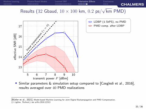
Results (32 Gbaud, 10 × 100 km, 0.2 ps/√
km PMD)
transmit power P [dBm]
effec
tive
SN
R[d
B]
23
24
25
26
27
5 6 7 8 9 10
uT
uT
uT
uT
uT
uT
uT
uTuT uT
uT
uT
uT
uT
rS
rS
rSrS
rS
rS
rS
rS
rS
rS
rS
rS
rS
rS
linea
rtr
ansm
ission
(γ=
0)
LDBP (4 StPS), no PMDrS
PMD comp. after LDBPuT
• Similar parameters & simulation setup compared to [Czegledi et al., 2016],results averaged over 40 PMD realizations
[Bütler et al., 2021], Model-based Machine Learning for Joint Digital Backpropagation and PMD Compensation,(J. Lightw. Technol.), see arXiv:2010.12313
33 / 36
Machine Learning Physics-Based Models Learned DBP Polarization Effects Conclusions
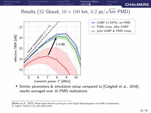
Results (32 Gbaud, 10 × 100 km, 0.2 ps/√
km PMD)
transmit power P [dBm]
effec
tive
SN
R[d
B]
23
24
25
26
27
5 6 7 8 9 10
uT
uT
uT
uT
uT
uT
uT
uTuT uT
uT
uT
uT
uT
lD
lD
lDlDlD
lD
lD
lD
lD
lD
lD
lD
lD
lD
rS
rS
rSrS
rS
rS
rS
rS
rS
rS
rS
rS
rS
rS
linea
rtr
ansm
ission
(γ=
0)
1.9 dB
LDBP (4 StPS), no PMDrS
joint LDBP & PMD comp.lDPMD comp. after LDBPuT
• Similar parameters & simulation setup compared to [Czegledi et al., 2016],results averaged over 40 PMD realizations
[Bütler et al., 2021], Model-based Machine Learning for Joint Digital Backpropagation and PMD Compensation,(J. Lightw. Technol.), see arXiv:2010.12313
33 / 36
Machine Learning Physics-Based Models Learned DBP Polarization Effects Conclusions
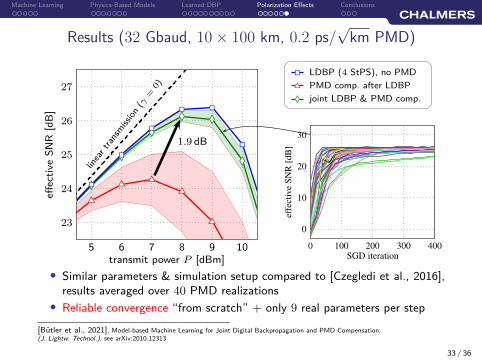
Results (32 Gbaud, 10 × 100 km, 0.2 ps/√
km PMD)
transmit power P [dBm]
effec
tive
SN
R[d
B]
23
24
25
26
27
5 6 7 8 9 10
uT
uT
uT
uT
uT
uT
uT
uTuT uT
uT
uT
uT
uT
lD
lD
lDlDlD
lD
lD
lD
lD
lD
lD
lD
lD
lD
rS
rS
rSrS
rS
rS
rS
rS
rS
rS
rS
rS
rS
rS
linea
rtr
ansm
ission
(γ=
0)
SGD iteration
eff
ecti
ve
SN
R[d
B]
0
10
20
30
0 400100 200 300
1.9 dB
LDBP (4 StPS), no PMDrS
joint LDBP & PMD comp.lDPMD comp. after LDBPuT
• Similar parameters & simulation setup compared to [Czegledi et al., 2016],results averaged over 40 PMD realizations
• Reliable convergence “from scratch” + only 9 real parameters per step
[Bütler et al., 2021], Model-based Machine Learning for Joint Digital Backpropagation and PMD Compensation,(J. Lightw. Technol.), see arXiv:2010.12313
33 / 36
Machine Learning Physics-Based Models Learned DBP Polarization Effects Conclusions
Outline
1. Machine Learning and Neural Networks for Communications
2. Physics-Based Machine Learning for Fiber-Optic Communications
3. Learned Digital Backpropagation
4. Polarization-Dependent Effects
5. Conclusions
34 / 36
Machine Learning Physics-Based Models Learned DBP Polarization Effects Conclusions
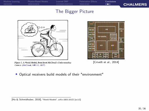
The Bigger Picture
[Crivelli et al., 2014]
• Optical receivers build models of their "environment"
[Ha & Schmidhuber, 2018], "World Models", arXiv:1803.10122 [cs.LG]
35 / 36
Machine Learning Physics-Based Models Learned DBP Polarization Effects Conclusions
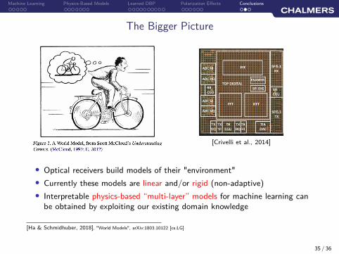
The Bigger Picture
[Crivelli et al., 2014]
• Optical receivers build models of their "environment"
• Currently these models are linear and/or rigid (non-adaptive)
• Interpretable physics-based “multi-layer” models for machine learning canbe obtained by exploiting our existing domain knowledge
[Ha & Schmidhuber, 2018], "World Models", arXiv:1803.10122 [cs.LG]
35 / 36

Machine Learning Physics-Based Models Learned DBP Polarization Effects Conclusions
Conclusions
36 / 36
Machine Learning Physics-Based Models Learned DBP Polarization Effects Conclusions
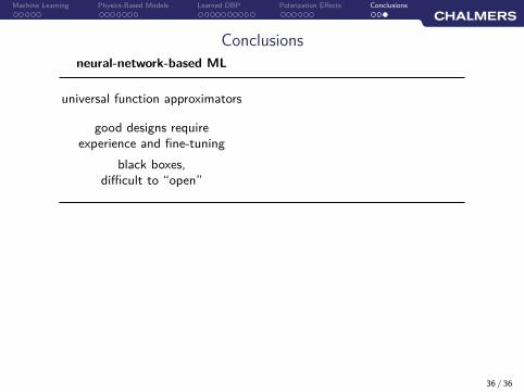
Conclusionsneural-network-based ML
universal function approximators
good designs requireexperience and fine-tuning
black boxes,difficult to “open”
36 / 36
Machine Learning Physics-Based Models Learned DBP Polarization Effects Conclusions
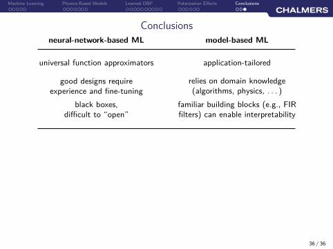
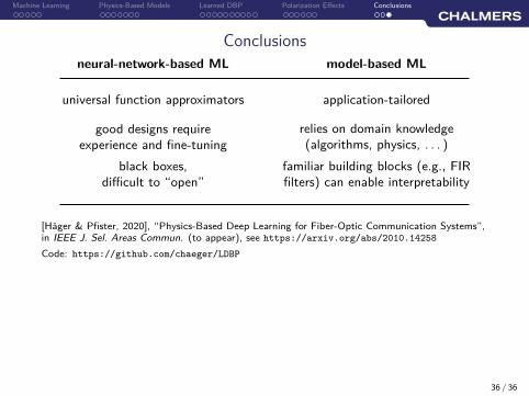
Conclusionsneural-network-based ML model-based ML
universal function approximators application-tailored
good designs requireexperience and fine-tuning
relies on domain knowledge(algorithms, physics, . . . )
black boxes,difficult to “open”
familiar building blocks (e.g., FIRfilters) can enable interpretability
36 / 36
Machine Learning Physics-Based Models Learned DBP Polarization Effects Conclusions
Conclusionsneural-network-based ML model-based ML
universal function approximators application-tailored
good designs requireexperience and fine-tuning
relies on domain knowledge(algorithms, physics, . . . )
black boxes,difficult to “open”
familiar building blocks (e.g., FIRfilters) can enable interpretability
[Häger & Pfister, 2020], “Physics-Based Deep Learning for Fiber-Optic Communication Systems”,in IEEE J. Sel. Areas Commun. (to appear), see https://arxiv.org/abs/2010.14258
Code: https://github.com/chaeger/LDBP
36 / 36
Machine Learning Physics-Based Models Learned DBP Polarization Effects Conclusions
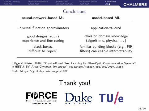
Conclusionsneural-network-based ML model-based ML
universal function approximators application-tailored
good designs requireexperience and fine-tuning
relies on domain knowledge(algorithms, physics, . . . )
black boxes,difficult to “open”
familiar building blocks (e.g., FIRfilters) can enable interpretability
[Häger & Pfister, 2020], “Physics-Based Deep Learning for Fiber-Optic Communication Systems”,in IEEE J. Sel. Areas Commun. (to appear), see https://arxiv.org/abs/2010.14258
Code: https://github.com/chaeger/LDBP
Thank you!
36 / 36
References I
Crivelli, D. E., Hueda, M. R., Carrer, H. S., Del Barco, M., López, R. R., Gianni, P., Finochietto, J.,
Swenson, N., Voois, P., and Agazzi, O. E. (2014).Architecture of a single-chip 50 Gb/s DP-QPSK/BPSK transceiver with electronic dispersion compensationfor coherent optical channels.IEEE Trans. Circuits Syst. I: Reg. Papers, 61(4):1012–1025.
Czegledi, C. B., Liga, G., Lavery, D., Karlsson, M., Agrell, E., Savory, S. J., and Bayvel, P. (2016).
Polarization-mode dispersion aware digital backpropagation.In Proc. European Conf. Optical Communication (ECOC), Düsseldorf, Germany.
Du, L. B. and Lowery, A. J. (2010).
Improved single channel backpropagation for intra-channel fiber nonlinearity compensation in long-hauloptical communication systems.Opt. Express, 18(16):17075–17088.
Essiambre, R.-J. and Winzer, P. J. (2005).
Fibre nonlinearities in electronically pre-distorted transmission.In Proc. European Conf. Optical Communication (ECOC), Glasgow, UK.
Häger, C. and Pfister, H. D. (2018a).
Deep learning of the nonlinear Schrödinger equation in fiber-optic communications.In Proc. IEEE Int. Symp. Information Theory (ISIT), Vail, CO.
Häger, C. and Pfister, H. D. (2018b).
Nonlinear interference mitigation via deep neural networks.In Proc. Optical Fiber Communication Conf. (OFC), San Diego, CA.
37 / 36
References II
He, K., Zhang, X., Ren, S., and Sun, J. (2015).
Deep residual learning for image recognition.
Ip, E. and Kahn, J. M. (2008).
Compensation of dispersion and nonlinear impairments using digital backpropagation.J. Lightw. Technol., 26(20):3416–3425.
Ip, E. and Kahn, J. M. (2009).
Nonlinear impairment compensation using backpropagation.In Optical Fiber New Developments, Chapter 10. IntechOpen, London, UK.
Lavery, D., Ives, D., Liga, G., Alvarado, A., Savory, S. J., and Bayvel, P. (2016).
The benefit of split nonlinearity compensation for single-channel optical fiber communications.IEEE Photon. Technol. Lett., 28(17):1803–1806.
LeCun, Y., Bengio, Y., and Hinton, G. (2015).
Deep learning.Nature, 521(7553):436–444.
Leibrich, J. and Rosenkranz, W. (2003).
Efficient numerical simulation of multichannel WDM transmission systems limited by XPM.IEEE Photon. Technol. Lett., 15(3):395–397.
Li, L., Tao, Z., Dou, L., Yan, W., Oda, S., Tanimura, T., Hoshida, T., and Rasmussen, J. C. (2011).
Implementation efficient nonlinear equalizer based on correlated digital backpropagation.In Proc. Optical Fiber Communication Conf. (OFC), Los Angeles, CA.
38 / 36
References III
Li, X., Chen, X., Goldfarb, G., Mateo, E., Kim, I., Yaman, F., and Li, G. (2008).
Electronic post-compensation of WDM transmission impairments using coherent detection and digital signalprocessing.Opt. Express, 16(2):880–888.
Li, Y., Ho, C. K., Wu, Y., and Sun, S. (2005).
Bit-to-symbol mapping in LDPC coded modulation.In Proc. Vehicular Technology Conf. (VTC), Stockholm, Sweden.
Lin, H. W., Tegmark, M., and Rolnick, D. (2017).
Why does deep and cheap learning work so well?J. Stat. Phys., 168(6):1223–1247.
Mnih, V., Kavukcuoglu, K., Silver, D., Rusu, A. A., Veness, J., Bellemare, M. G., Graves, A., Riedmiller, M.,
Fidjeland, A. K., Ostrovski, G., Petersen, S., Beattie, C., Sadik, A., Antonoglou, I., King, H., Kumaran, D.,Wierstra, D., Legg, S., and Hassabis, D. (2015).Human-level control through deep reinforcement learning.Nature, 518(7540):529–533.
Nakashima, H., Oyama, T., Ohshima, C., Akiyama, Y., Tao, Z., and Hoshida, T. (2017).
Digital nonlinear compensation technologies in coherent optical communication systems.In Proc. Optical Fiber Communication Conf. (OFC), Los Angeles, CA.
Napoli, A., Maalej, Z., Sleiffer, V. A. J. M., Kuschnerov, M., Rafique, D., Timmers, E., Spinnler, B.,
Rahman, T., Coelho, L. D., and Hanik, N. (2014).Reduced complexity digital back-propagation methods for optical communication systems.J. Lightw. Technol., 32(7):1351–1362.
39 / 36

References IV
O’Shea, T. and Hoydis, J. (2017).
An introduction to deep learning for the physical layer.IEEE Trans. Cogn. Commun. Netw., 3(4):563–575.
Paré, C., Villeneuve, A., Bélanger, P.-A. A., and Doran, N. J. (1996).
Compensating for dispersion and the nonlinear Kerr effect without phase conjugation.Opt. Lett., 21(7):459–461.
Pillai, B. S. G., Sedighi, B., Guan, K., Anthapadmanabhan, N. P., Shieh, W., Hinton, K. J., and Tucker,
R. S. (2014).End-to-end energy modeling and analysis of long-haul coherent transmission systems.J. Lightw. Technol., 32(18):3093–3111.
Rafique, D., Zhao, J., and Ellis, A. D. (2011).
Digital back-propagation for spectrally efficient wdm 112 gbit/s pm m-ary qam transmission.Opt. Express, 19(6):5219–5224.
Roberts, K., Li, C., Strawczynski, L., O’Sullivan, M., and Hardcastle, I. (2006).
Electronic precompensation of optical nonlinearity.IEEE Photon. Technol. Lett., 18(2):403–405.
Secondini, M., Rommel, S., Meloni, G., Fresi, F., Forestieri, E., and Poti, L. (2016).
Single-step digital backpropagation for nonlinearity mitigation.Photon. Netw. Commun., 31(3):493–502.
Sheikh, A., Fougstedt, C., Graell i Amat, A., Johannisson, P., Larsson-Edefors, P., and Karlsson, M. (2016).
Dispersion compensation FIR filter with improved robustness to coefficient quantization errors.J. Lightw. Technol., 34(22):5110–5117.
40 / 36

References V
Yan, W., Tao, Z., Dou, L., Li, L., Oda, S., Tanimura, T., Hoshida, T., and Rasmussen, J. C. (2011).
Low complexity digital perturbation back-propagation.In Proc. European Conf. Optical Communication (ECOC), page Tu.3.A.2, Geneva, Switzerland.
41 / 36