model behavior and the strengths of causal loops ... · model behavior and the strengths of causal...
TRANSCRIPT

Model Behavior and the Strengths of Causal Loops:
Mathematical Insights and a Practical Method
John HaywardDivision of Mathematics and Statistics, University of Glamorgan,
Pontypridd, CF37 1DL, Wales, UK
(+44)1443 654370, [email protected]
Presented at the 30th International System Dynamics Conference
St Gallen, Switzerland, 2012
Abstract
Quantifying the strength of causal loops on a stock can help bring insights intothe relationship between model structure and behavior. This paper uses mathe-matics to derive loop strengths in a number of generic small models using therelationship between the second and first derivative from the Pathway Partici-pation Metric method. The loop strengths are plotted in a System Dynamics(SD) simulator together with the stocks to help explain behavior in the Limits toGrowth, Predator-Prey, Diffusion and SIR models among others. Issues such asloop dominance, flow dominance and the change of polarity of higher order loopsare used to explain behavior. In particular the identity of the causal loops in theDiffusion and SIR models are discussed and compared with previous work. Fi-nally a numerical method for computing loop strengths and identifying dominantloops within an SD simulator is presented and applied to the Yeast Model. It ishoped that the paper will inspire others to use loop strengths in their analysis andunderstanding of SD models.
Key Words: System dynamics, causal loops, SIR model, yeast model, loop dom-inance, pathway participation metric.
1 Introduction
1.1 Model Structure and System Dynamics
A central premise of system dynamics is that dynamical behavior can be explained by modelstructure. Recently Richardson (2011) characterized the field of system dynamics as:
System dynamics is the use of informal maps and formal models with computersimulation to uncover and understand endogenous sources of system behavior.
1

The “informal maps” include the causal loops of the more formal system dynamics modelwhich provide a powerful and intuitive explanation of model behavior in terms of its struc-ture. The formal system dynamics model is however more than causal loops, it consists ofthe feedback loops, stocks, flows and non-linearities created by the interaction of the physicaland institutional structure of the system with the decision making processes of the agentsacting within it (Sterman, 2000, p.107). Feedback loops are essential as these are key tothe endogeneity of the system, the main feature that determines the power of the modelto explain phenomena (Richardson, 2011). However they are not the only element thatdetermines structure, in addition there are the stock (level) variables that represent accumu-lations and the flow (rate) variables that represent activity within the feedback loops (e.g.Forrester, 1968a, as quoted in Richardson, 2011).
As such, feedback loops are not sufficient to explain system behavior alone; the stocksand flows of the system need to be identified in order to capture its full structure andhence explain its full behavior. The system dynamics (SD) model is that interconnectednetwork of entities that includes rate and accumulation relationships in addition to algebraicconnections and delays. The model can be reduced to causal loop diagrams in order to explainbehavior in a simple and intuitive way, but the loss of information about accumulations,and the flow structure, runs the risk of confusing and incorrect explanations (Richardson1986; 1995; 1997). Additionally the SD model can be reduced to a set of ordinary differentialequations for more a mathematical analysis. However, although this retains the stock/flowrelationship in the integration, it loses some of the causal structure, which is precisely theinformation the system dynamicist hopes to use to explain the behavior. An SD model ismore than a set of causal loops and more than a set of differential equations. Both arerequired to do justice to the word “structure” in the SD model.
1.2 Problems Using Causal Loops to Explain Behavior
The fact that causal loops do not capture all the structure in an SD model can lead toproblems if they alone are used to interpret the model’s behavior:
1. The presence of a stock/flow combinations in the loop. Every causal loopmust have at least one stock, and thus at least one flow. As such at least one causallink in the loop is a material (additive) one where positive polarity means “add to”,rather than an information (proportional) link, where it means “change the same way”(Richardson 1986; 1997). Whereas an information link can be reversed, a materiallink may not be, unless there are other processes that affect the stock. For example ifx is connected to a stock y with positive polarity then reducing x does not reduce ybut adds less to it. Thus unless there are other processes removing material from y,reducing x means y increases more slowly.
2. The relative strengths of the causal loops. The mere presence of a loop in acausal loop diagram does not guarantee that it is significant in explaining the behaviorof the system. Loops have different strengths and some are more important thanothers. This has led to methods to search for dominant loops and structures (Ford,1999; Mojtahedzadeh et.al., 2004; Kampmann & Oliva, 2011).
3. The degree of non-linearity of a loop. If an effect has two or more causes then the
2

mechanism that describes their combination may be non-linear, e.g. multiplicative.This leads to loops having variable strength and thus loop dominance will changeover time. Additionally this may lead to bifurcations and a resulting change of mode(Richardson, 1995).
4. The order of a loop. That is the number of stocks in the loop. Although a secondor higher order loop has a fixed polarity, the effect of the loop on an individual stockat a given time may change its polarity. For example if x and y are both stocksin a reinforcing loop with positive links, an increase in x will add more to y. Butif y has other processes reducing its level at a faster rate than any of its inflows,then y will continue to decrease, albeit slower, and thus its effect on x is to slowits growth, a negative effect. Thus non-first order loops may flip their polarity ona given stock as net flows change sign. Such behavior is the source of oscillations(Richardson, 1995; Mojtahedzadeh & Richardson, 1995).
5. Confusion over the number of loops in the system. For example the SIR modelfor the spread of a disease can be constructed with two, three or more loops, butwith identical behavior across the models. Although the extra loops help explain theconstruction of the model they do not appear to help explain its behavior (Lyneis &Lyneis, 2006).
1.3 Quantitative Approaches to Causal Loops
In the light of the problems encountered using causal loop diagrams it would be useful if theeffect of the loops, and other structures, could be quantified. Kampmann & Oliva (2011)review the current state methods for structural dominance, to which the reader is referred.Briefly there are four types of methods: Traditional control theory; pathway participationmetrics (e.g. Mojtahedzadeh et.al., 2004); eigenvalue elasticity analysis (e.g. Kampmann,1996) and eigenvectors & dynamic decomposition weights (e.g. Guneralp, 2005).
In addition there are a number of behavioral methods for the detection of dominant structuressuch as loop deactivation (Ford, 1999; Phaff, 2008; Huang, 2009), and tracking loop gains(Kim, 1995). These have the advantage over the more formal methods in that they can beincorporated into propriety SD simulation software and do not require the use of advancedmathematical techniques or bespoke tools.
Although all the methods shed insight on the quantitative behavior of loops and structurethey only give a partial description of behavior. Perhaps for this reason, and also thecomplexity of their application, no method is as yet in widespread use in the SD community.This is a continuing area for research.
1.4 Outline of Paper
This paper intends to shed some light on the method used in the pathway participation metric(PPM) to help relate causal loop structure to behavior. The specific aims of the paper aretwo-fold: To investigate mathematically causal loop strengths, incorporating them in SDsimulations to help explain stock behavior; to develop a practical method of incorporating
3

the numerical derivation of the loop strengths in a propriety SD simulator to allow their usewithout the need for mathematical calculation. The purpose is to develop a method thatcan provide insight into the relationship between structure and behavior at different phasesof a system’s history.
The method is outlined in section 2. The models are kept deliberately simple in order towiden the accessibility of the method. Additionally the models used are generic to simplifythe mathematical analysis and focus on essential model structure. All the models havebeen implemented in Stella1, including plots of loop strengths and the identification of loopdominance. For clarity the models and graphs in the mathematical sections (3–5) have beenre-presented but all have their counterparts in Stella.
The practical method is illustrated (section 6) with the well known Yeast Model. In thissection, and the associated appendix, Stella notation and graphs are retained to help thereader use the method in conjunction with the SD model.
2 Outline of Method
The behavior of any element in a system dynamics model is partly determined by the struc-ture of the feedback loops through that element. A feedback loop must contain at leastone stock, call it x. In order to obtain the effect of a particular loop on the behavior ofx the question can be asked: if x increases what is the subsequent effect of that increaseon x itself; does it change faster or does it change slower as a result of that initial change?The former is a reinforcing loop where there is acceleration, and the latter a balancing one,where there is retardation. Essentially this question explores the link between the change inx, i.e. the derivative, or net flow, x, and the second derivative, or curvature, x. It is this re-lationship that underlies the pathway participation metric (PPM) method (Mojtahedzadehet.al., 2004); Richardson’s (1995) description of loop polarity and Ford’s (1999) behavioralapproach to loop dominance.
However the feedback loops are not the only type of structure that determines the behaviorof the stock x, the net flow will govern whether x is increasing, decreasing, or stationary atany time. Thus the sign of x also needs to be considered in order to understand behavior.Thus four types of “structure” can be identified: R+, R−, B+ and B−, where the letter refersto the nature of the feedback loop and the sign refers to the net flow of x. There are fouratomic behavior patterns associated with these structures: accelerating growth, acceleratingdecline, decelerating growth and decelerating decline (figure 1). Ford (1999) refers to thefirst two as exponential with an index of +1, and the latter two as logarithmic with anindex of -1. The sign of x is not indicated in the behavioral method as it concentrates onidentifying dominant loops, irrespective of growth or decline. If the cases of either or boththe first and second derivatives being equal to zero are considered then up to nine atomicbehavior patterns can be identified (Kampmann & Oliva, 2011). As the extra cases oftenonly occur at a critical point when a derivative is changing sign these will be omitted forsimplicity.
1Stella is produced by isee systems, USA. www.iseesystems.com
4

R+
B+ B-
R-
Fig. 1: Atomic Behavior Patterns Associated with Loop and Flow Structure.
For a first order autonomous system (1):
x = f(x) (1)
where f(x) represents the relationships between the stock x ≥ 0 and its flows. The relation-ship between the first and second derivative of x, and thus the loops, can be identified bydifferentiation:
x = f ′(x)x =m∑k=1
Akx (2)
f ′(x) will identify the number m, polarity and strengths of the causal loops Ak (Richardson,1995; Mojtahedzadeh et.al., 2004). In this definition the strength of a loop is a measure ofits effect on the target stock x.
For a higher order system the situation is more complex as at least one loop will have twoor more stocks and thus place a delay in the loop. For a second order system with stocks x,y:
x = f(x, y) (3)
y = g(x, y) (4)
Differentiating (3) gives the relationship between the first and second derivatives of x:
x =∂f
∂xx +
∂f
∂yy =
∂f
∂xx +
∂f
∂y
dy
dxx =
∂f
∂xx +
∂f
∂y
g
fx (5)
using the chain rules for partial and total differentiation and substituting from equations(3–4). The first term ∂f/∂x will identify the first order loops for a given f once the partialderivative is decomposed into different terms, as in (2). The second term (∂f/∂y)(g/f)will contain the effects of the second order loops, but may also contain effects on x from ythat are exogenous and not part of any of its loops. This will be explored in the examples.
5

Equation (5) is a special case of equation (4) in (Mojtahedzadeh et.al., 2004), the nth ordersystem. A similar equation can be identified for the effects of the loops on y.
Once the partial derivatives are decomposed into loops the different strengths of the loops ona given stock can be identified. In the PPM method a metric is defined that gives the relativestrength of each loop in order to identify dominant structures. In this paper the actual valuesof the strengths will be derived and examined as issues other than loop dominance will beconsidered, such as the contrast with net flow.
3 First Order Models
3.1 Compounding and Draining Process
Consider the standard compounding and draining process, with a constant outflow, figure 2with corresponding equation (6).
x
x inflow x outflow
a b
e
+ +R B
Fig. 2: Compounding and Draining Process, SD Model.
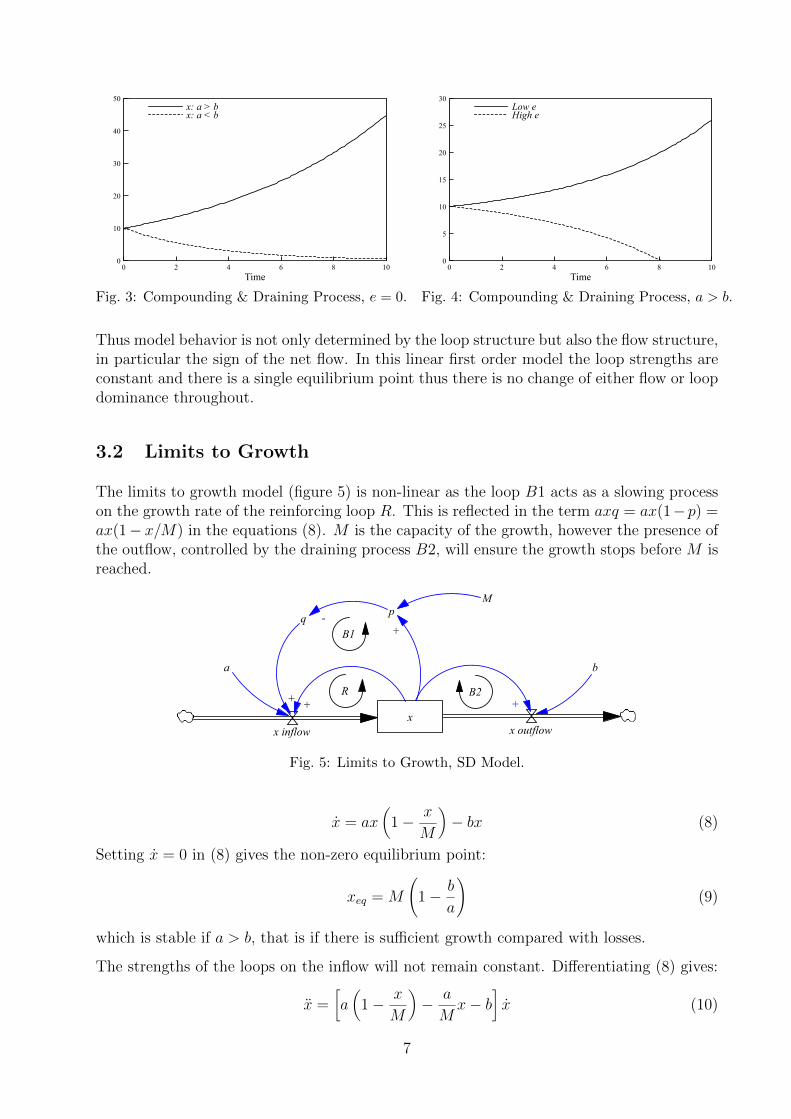
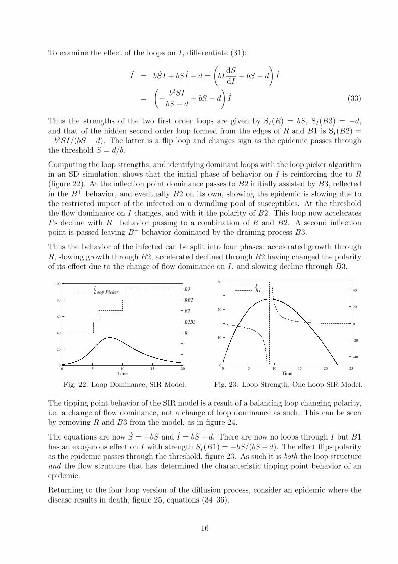
x = ax− bx− e (6)
It is assumed x ≥ 0. The model is linear with a reinforcing loop R and balancing loop B.This model is considered first as the constant loop dominance will be a contrast to the latermore complex models.
Differentiating (6) gives:x = (a− b)x (7)
showing the strengths and polarity of the loops, S(R) = a and S(B) = −b. The strengths areconstant due to the linearity of the system. Thus one loop is always dominant throughout(unless a = b), and the behavior of the system is determined by which loop is the stronger.For example, in figure 3, a > b, e = 0, thus the reinforcing loop dominates |S(R)| > |S(B)|,with R+ behavior. For a < b, e = 0 the balancing loop dominates with B− behavior. Thusincreasing b has not only changed the loop dominance but also the flow dominance of x, fromgrowth to decline. The equilibrium point at xeq = 0 has changed from unstable to stable.
Although the outflow e has no effect on loop dominance its value does effect the flow domi-nance of x. In figure 4 both curves have a > b thus the reinforcing loop is dominant in both.However the dashed curve has a higher value of the constant outflow e and thus the behaviorhas changed from R+ to R−. The equilibrium point xeq = e/(a− b) remains unstable, thusif the initial value x0 > xeq then x > 0 and the behavior is R+, and if x0 < xeq then x < 0and the behavior is R−.
6
0 2 4 6 8 10Time
0
10
20
30
40
50x: a > bx: a < b
Fig. 3: Compounding & Draining Process, e = 0.
0 2 4 6 8 10Time
0
5
10
15
20
25
30Low eHigh e
Fig. 4: Compounding & Draining Process, a > b.
Thus model behavior is not only determined by the loop structure but also the flow structure,in particular the sign of the net flow. In this linear first order model the loop strengths areconstant and there is a single equilibrium point thus there is no change of either flow or loopdominance throughout.
3.2 Limits to Growth
The limits to growth model (figure 5) is non-linear as the loop B1 acts as a slowing processon the growth rate of the reinforcing loop R. This is reflected in the term axq = ax(1−p) =ax(1− x/M) in the equations (8). M is the capacity of the growth, however the presence ofthe outflow, controlled by the draining process B2, will ensure the growth stops before M isreached.
x
x inflow x outflow
a b
+ +
R B2
pq
M
+
-
+
B1
Fig. 5: Limits to Growth, SD Model.
x = ax(
1− x
M
)− bx (8)
Setting x = 0 in (8) gives the non-zero equilibrium point:
xeq = M
(1− b
a
)(9)
which is stable if a > b, that is if there is sufficient growth compared with losses.
The strengths of the loops on the inflow will not remain constant. Differentiating (8) gives:
x =[a(
1− x
M
)− a
Mx− b
]x (10)
7

where the structure of the model has been preserved in the differentiation of the first term.That is the product rule is used on x(1 − x/M) without multiplying out the brackets.Thus (10) identifies the strengths of each loop: S(R) = a(1 − x/M), S(B1) = −ax/Mand S(B2) = −b. Clearly as x increases |S(R)| will decrease and |S(B1)| will increase. Ifthe system starts with R dominant then it will eventually change to the balancing loopsdominating. This is shifting loop dominance, figure 6.
0 5 10 15 20 25Time
0
2
4
6
8
10
12
14 xR | B1B2B1B2 | B1
Fig. 6: Loop Dominance, Limits to Growth.
0 5 10 15 20 25Time
0
0.1
0.2
0.3
0.4RB1 B2B1B2
Fig. 7: Loop Strengths, Limits to Growth.
The absolute loop strengths |S(R)|, |S(B1)| and |S(B2)| can be computed and plotted withinan SD simulation, figure 7. In order to identify the dominant loop or loop combination, thesum of the two balancing loops is also computed. It can be seen that there are three phases.Firstly the reinforcing loop R dominates to the point that it drops below the B1B2 curve.Secondly the sum of the two balancing loops dominates over R until the B1 curve exceedsthe R curve figure 7. In this third phase B1 is strong enough to dominate R on its own.
The three phases can be indicated on the same graph as the plot of x, the vertical linesR|B1B2, B1B2|B1, representing the transitions, figure 6. These lines are constructed usingthe loop picker algorithm on the causal loop strengths (see section 6 and appendix). Thetransition from R to both balancing loops dominating together occurs at the inflection point.
4 Higher Order Models
4.1 Second Order Linear Model
In a second order model it is now possible for a stock to feedback on itself via another stock.Consider the system with one first order balancing loop that attempts to adjust a stock xtoward a target y, with a second order reinforcing loop that causes the target y to increaseas x increases, figure 8 and equations (11–12)
x = a(y − x) (11)
y = cx (12)
Differentiating (11) derives the strength of the two causal loops that affect x:
x = ay − ax =(ay
x− a
)x =
(cx
y − x− a
)x (13)
8

x
x inflow
a
R
B
y
c
gap
-
+
y infow
+
+
Fig. 8: 2nd Order Model.
Thus the reinforcing and balancing loop have strength:
S(R) =cx
y − x(14)
S(B) = −a (15)
where the chain rule has been used to derive the instantaneous effect of the second orderloop on x, called an implicit loop by Mojtahedzadeh & Richardson (1995).
0 5 10 15 20Time
0
0.1
0.2
0.3
0.4
0.5
0.6
0.7
RB
Fig. 9: Loop Strengths, 2nd Order Model.
0 5 10 15 20Time
0
10
20
30
40
50
60
70xyB | R
R+
B+
Fig. 10: Loop Dominance, 2nd Order Model.
The balancing loop is constant as it is a linear first order loop. However the reinforcingloop has a variable effect on x because it is second order and its impact is delayed. Thusthere are scenarios where the constant balancing loop B dominates initially, but is eventuallyovertaken by the growing reinforcing loop, figure 9. Thus the behavior of x is initially B+,followed by R+ as the delayed reinforcing loop dominates, figure 10. The vertical line B|Rmarks the change of dominance. Note that y only has a reinforcing loop and is always R+.
To confirm the above analysis by causal loops, a stability analysis shows that the equilibriumpoint is a saddle instability. The solution for x is of the form x = C1e
−m1t + C2em2t, where
m1,m2 > 0. If m1 � m2 the declining exponential dominates initially, the balancing effect,but the growing exponential always dominates ultimately. The relative values of m1,m2
govern the delay in the second order reinforcing loop.
With y having a similar form to x, y = C3e−m1t +C4e
m2t, then as t increases, the reinforcing
9

loop (15) tends to a constant value:
S(R) =cx
y − x≈ cC2e
m2t
C2em2t − C4em2t=
cC2
C2 − C4
as shown in figure 9. However, although the solution has confirmed the causal loop analysis,the plots of the strengths of the loops, figure 9, are sufficient to explain the behavior, figure10, in terms of structure.
4.2 Dominance of Non Loop Structures
Although computing the second derivative (13) has picked up the effect of the second orderloop on x, strictly speaking the first term is due to the overall effect of y on x regardless ofwhether y is in a loop through x or not. For example, breaking the link from x to the inflowof y and replacing it by a first order reinforcing loop from y gives only one causal loop forx, (figure 11 and equations (16 –17)):
x
x inflow
a
R
B
y
c
gap
-
+
y infow
+
Fig. 11: Second Order Model with a Reinforcing Loop Exogenous to x.
x = a(y − x) (16)
y = cy (17)
Although there is only one loop through x there are still two terms in the curvature of x,x = (cy/(y − x)− a)x as the now exogenous system in y still affects x.
The resulting behavior for x is identical to the endogenous system as the reinforcing loopthrough y only is reflected in x. It needs to be remembered that the causal loops througha variable are not the only structures that determine behavior. In this case the curvatureanalysis has picked up the effect of the exogenous stock/flow structure on the stock x. Thusin this case of exogenous behavior it would be more correct to refer to structural dominanceon x as the second phase is dominated by a reinforcing loop not through x itself, (seeKampmann & Oliva, 2011).
4.3 Oscillating Systems
Endogenous oscillation can occur when the restorative effect of a balancing loop is delayeddue to the presence of extra stocks in the loop. Consider the standard Volterra predator
10

0 5 10 15 20Time
0
10
20
30
40
50
60
70xyB | R
B+
R+
Fig. 12: Structural Dominance in a Second Order Model with a Reinforcing Loop Exogenous to x.
-prey system when x is the prey and y is the predator, figure 13 equations (18–19).
x
x inflow
a
B3
B1
y
c
y infow
x outflow
y outflow
b
d
+
R1
B2 R2
Fig. 13: Predator-Prey System, SD Model.
x = ax− bxy (18)
y = cxy − dy (19)
All the loops are first order except B3 which is second order.To find its instantaneous effecton the stock x, differentiate (18):
x = ax− bxy − byx =
(a− bx
dy
dx− by
)x
=
(a− b
y(cx− d)
(a− by)− by
)x (20)
The first and last terms are the first order loops through the prey x: S(R1) = a, S(B1) = −by.The second order balancing loop has a more complex instantaneous strength
S(B3) = −by(d− cx)
(b− ay)(21)
11

which may take both positive and negative values. Thus although it is a balancing loop theeffect of its higher order is to delay the corrective action and thus induce a succession of B−,R+, B+, R− behavior on x, typical of an oscillation, (the curve in figure 14). The loop B3has a variable polarity in terms of its effect on x, i.e. as an implicit loop (Mojtahedzadeh &Richardson, 1995). Such loops will be referred to as flip loops in this paper as they have thepotential to flip polarity, depending on the flow dominance of x and y.
Using the loop picker algorithm (section 6 and appendix) the regions of loop dominancecan be determined, showing in some regions B3 is having a balancing effect and may becombined with B1, and in other regions B3 is having a reinforcing effect and is sometimescombined with R1. Initially B1 dominates, figure 14, followed by B3, as its effect is negative(figure 15) and the x curve is B−. B3 remains dominant throughout the minimum point.The curve for x becomes R+, as the flow dominance on x switches from negative to positiveand B3 has a positive effect on x (figure 15). The infinity in its strength at the turning pointis because at such a point x = 0, thus with this definition of loop strength, the subsequenteffect of a change in x on its curvature is ill defined as it is momentarily not changing2. Theloop is still balancing as it is still opposing the motion of x but its immediate effect on x isout of phase due to the delay of y and thus its sign changes, as the net flow changes sign.
0 10 20 30 40Time
1
2
3
4
5
6
R1
R1B3
B1
B3
B1B3xLoop Picker
Fig. 14: Loop Dominance, Predator Prey Model.
0 10 20 30 40Time
-1
0
1R1B1B3
Fig. 15: Loop Strengths, Predator Prey Model.
As B3 weakens, R1 becomes dominant. At the inflection point the R+ changes to B− andthus the balancing loops B1 and B3 become dominant. Note that the effect of B3 hasnow gone back to negative, (figure 15). Again B3 is dominant around the maximum point.Indeed, in this model, the turning points are not explained by a change of loop dominance,B3 is dominant in both, but by a change in flow dominance on x and a reversal of thepolarity of the second order loop B3.
It should be noted that there are phases where no single loop through x is dominatingits behavior. The second order loop B3 is sometimes combined with either R1 or B1 fordominance to occur, depending on its polarity. That polarity is partly determined by therelative strengths of R2 and B2 and thus it would be possible to uncover the relative impactof the five loops on the system as a whole, as in Mojtahedzadeh (2009a, figure 5).
2The infinity is normalized to unity in PPM as relative loop strengths are used
12

5 Diffusion and Epidemic Models
5.1 Issues in Diffusion models
The loops of the Bass product diffusion model have caused some discussion as to the number,and nature, of the loops through each stock (Lyneis & Lyneis, 2006; Kampmann & Oliva,2011). Taking the analogy of the spread of a disease let S be the susceptibles, or potentialcustomers and I the infected, or actual customers who spread information about the productby word of mouth. At its simplest the two loop version can be described as in figure 16,equation (22–23).
S
RB1
I
S to I
+ +
b
Fig. 16: Diffusion, SD Model.
S = −bSI (22)
I = bSI (23)
Considering the loops through I, differentiate (23):
I = bSI + bSI =
(bI
dS
dI+ bS
)I = (−bI + bS) I (24)
Thus two loops affect I, the reinforcing loop with strength SI(R) = bS and an effect whichis balancing with absolute strength bI. However it is not clear that this behavior can beidentified with B1, which is first order through S only. There are two ways this can beviewed:
1. There is an exogenous effect of the loop B1 on the inflow of I, rather like the situationin section 4.2.
2. There is second order loop between S and I which is hidden by the system dynamicsnotation of a conserved flow, as suggested by Mojtahedzadeh (2009b, figure 6a).
The second of these two is the preferred explanation, as the Bass model is a special case ofthe second order system where S and I have separate outflows (figure 17, equations 25–26)and b = c.
S = −bSI (25)
I = cSI (26)
The loop B2 is hidden by the conserved flow notation of system dynamics and only appearsin figure 16 as a figure of eight through R1 and B1. Thus for I the loops are SI(R) = bS andSI(B2) = −bI. The result is shifting loop dominance from R to B2 (figure 18), consistent
13

S
R
B1
b
S outflow
II inflow
B2
c
Fig. 17: Second Order Model that Reduces to Diffusion Model if b = c.
0 2 4 6 8 10Time
0
20
40
60
80
100IR | B2
Fig. 18: Diffusion Model, Loop Dominance.
0 2 4 6 8 10Time
0
50
100
150
200SB2 | B1
B-
R-B+
Fig. 19: Diffusion Model, Constant Inflow on S.
with the PPM analysis in Kampmann & Oliva (2011, figure 7). Note the Bass diffusionmodel has a similar explanation to the Limits to Growth model (section 3.2), as expectedbecause the two models reduce to the same differential equation, the logistic equation.
For the variable S the two loops are both balancing, SS(B1) = −bI and SS(B2) = bS.However the effect of B2 on S is reinforcing as S is decreasing, thus B2 is a flip loop. Theaddition of a constant inflow on S, S = a − bSI allows S to increase initially and for B2to behave in the orthodox fashion as B+ before changing to R− when the net flow on Schanges sign. Finally the behavior of S becomes B− as loop dominance changes from B2 toB1 (figure 19).
In the 4 loop version of the diffusion model, figure 20, the loops are defined via an in-termediate fraction or probability, S/N , where N = S + I (e.g. Lyneis & Lyneis, 2006,figure 6; Mojtahedzadeh, 2011, figure 1c), often referred to as the standard incidence model(Hethcote, 1994).The equations now become:
S = −b SNI = −b S
S + II (27)
I = bS
NI = b
S
S + II (28)
14

S
R1B1
I
S to I
+
b
S/N
N+ +
-
+
+
R2 B4
Fig. 20: Four Loop Diffusion, SD Model.
Two extra terms are generated for I:
I =(−b I
N+ b
S
N− b
SI
N2+ b
SI
N2
)I (29)
There are now two additional loops, B4, and R2 (these are shown in a later model, figure 25).Lyneis & Lyneis (2006) describe these extra loops, whose strengths are the last two termsin (29), as dynamically inactive and self canceling, the latter confirmed by the terms beingequal and opposite. Mojtahedzadeh (2011) applies the PPM method to this model using thesoftware Digest, explicitly showing the equal and opposite contributions of the two loops (seeMojtahedzadeh, 2011, table 2, where new reinforcing healthy loop is R2 and infected-healthypathway is B4). Thus these additional loops have no effect on either stock and they canbe effectively excluded in a discussion of loop dominance. This is a direct consequence ofthe flow being conserved, N = 0. The situation where the flow is not conserved will beconsidered under the SIR epidemic model (section 5.2).
5.2 SIR Epidemic Model
The SIR epidemic model is an extension of the diffusion model where the infected (actualcustomers) lose their infection and are no longer open to being infected again. Let S be thesusceptibles, I the infected and R the removed. The model now has an extra balancing loopB3, compared with the diffusion model, figure 21, equations (30–32).
S
RB1
I
S to I
+ +
b
R
I to R
+
B3
d
Fig. 21: SIR Epidemic, SD Model
S = −bSI (30)
I = bSI − dI (31)
R = dI (32)
15
To examine the effect of the loops on I, differentiate (31):
I = bSI + bSI − d =
(bI
dS
dI+ bS − d
)I
=
(− b2SI
bS − d+ bS − d
)I (33)
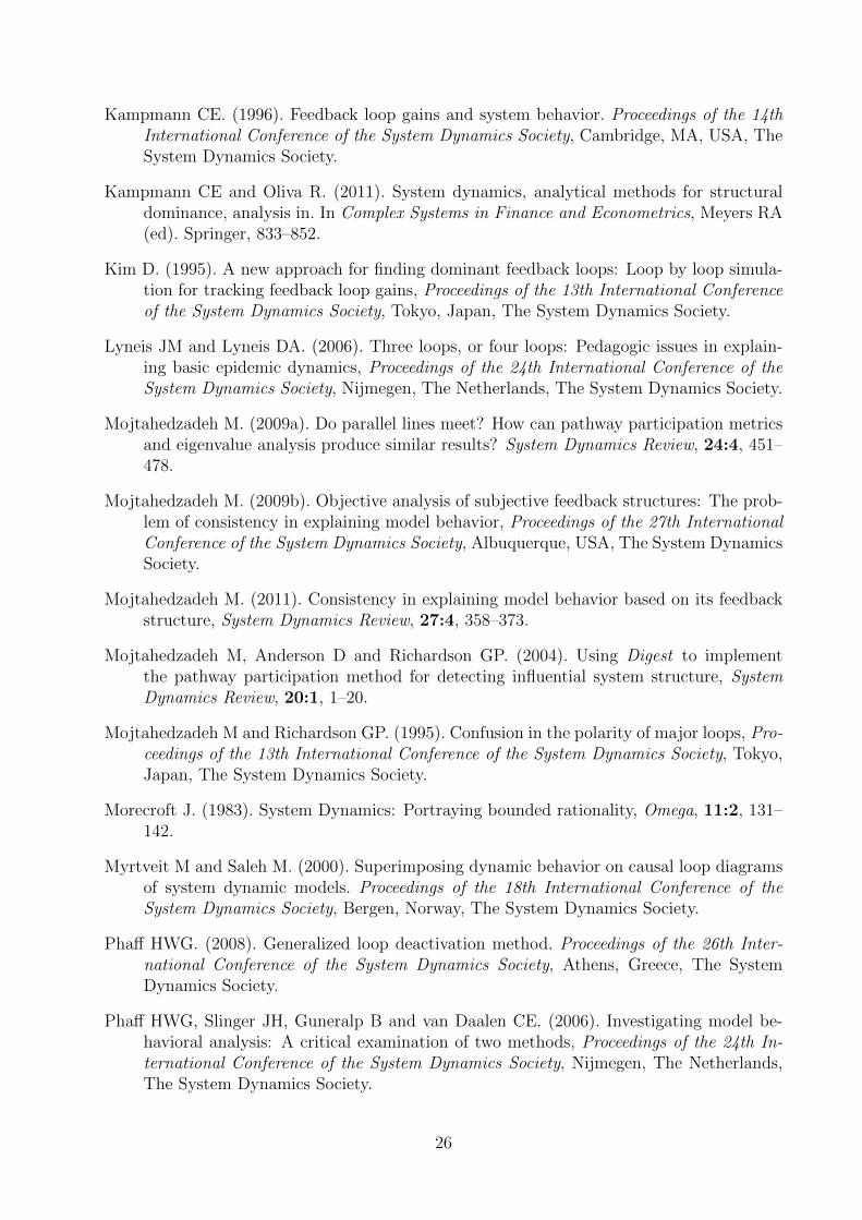
Thus the strengths of the two first order loops are given by SI(R) = bS, SI(B3) = −d,and that of the hidden second order loop formed from the edges of R and B1 is SI(B2) =−b2SI/(bS − d). The latter is a flip loop and changes sign as the epidemic passes throughthe threshold S = d/b.
Computing the loop strengths, and identifying dominant loops with the loop picker algorithmin an SD simulation, shows that the initial phase of behavior on I is reinforcing due to R(figure 22). At the inflection point dominance passes to B2 initially assisted by B3, reflectedin the B+ behavior, and eventually B2 on its own, showing the epidemic is slowing due tothe restricted impact of the infected on a dwindling pool of susceptibles. At the thresholdthe flow dominance on I changes, and with it the polarity of B2. This loop now acceleratesI’s decline with R− behavior passing to a combination of R and B2. A second inflectionpoint is passed leaving B− behavior dominated by the draining process B3.
Thus the behavior of the infected can be split into four phases: accelerated growth throughR, slowing growth through B2, accelerated declined through B2 having changed the polarityof its effect due to the change of flow dominance on I, and slowing decline through B3.
0 5 10 15 20Time
0
20
40
60
80
100
R
B2B3
B2
RB2
B3ILoop Picker
Fig. 22: Loop Dominance, SIR Model.
0 5 10 15 20 25Time
0
10
20
30
-40
-20
0
20
40IB1
Fig. 23: Loop Strength, One Loop SIR Model.
The tipping point behavior of the SIR model is a result of a balancing loop changing polarity,i.e. a change of flow dominance, not a change of loop dominance as such. This can be seenby removing R and B3 from the model, as in figure 24.
The equations are now S = −bS and I = bS − d. There are now no loops through I but B1has an exogenous effect on I with strength SI(B1) = −bS/(bS− d). The effect flips polarityas the epidemic passes through the threshold, figure 23. As such it is both the loop structureand the flow structure that has determined the characteristic tipping point behavior of anepidemic.
Returning to the four loop version of the diffusion process, consider an epidemic where thedisease results in death, figure 25, equations (34–36).
16

S
B1
I
S to I
+
b
R
I to R
d
Fig. 24: Cut down SIR model to Illustrate Tipping Point Behavior.
S
R1B1
I
S to I
+
b
I to R
+
B3
dS/N
N+ +
-
+
+
R2 B4
Fig. 25: SIR Standard Incidence Model with Deaths, N = S + I.
S = −b SNI (34)
I = bS
NI − dI (35)
R = dI (36)
Unlike the four loop Bass diffusion model N = S + I is no longer constant, N 6= 0, and theloops B4 and R2 will no longer be self canceling. Differentiating equation (35), gives, aftersome algebra:
I =
(bS
N− b2SI
bS − dN− d− bSI
n2+
b2S2I
n2(bS − dN)
)I (37)
where the loop strengths of R1, B2, B3, B4 and R2 are given by the consecutive terms inthe brackets of (37)3. By comparing the loop strengths in an SD simulation the differentphases of loop dominance on I can be identified using the loop picker, figure 26 and table 1.Although the many changes of structural dominance look complex, from a behavioral pointof view there are still only four phases:
1. R+, where R1 dominates, latterly assisted by R2;
2. B+, where the second order B2 dominates with negative effect on I, initially assistedby combinations of B3 and B4;
3. R−, where B2 remains dominant, but now with positive effect on I, assisted latterlyby R1;
3Strictly speaking it is not R2 that is through I but a hidden second order loop formed from it, in asimilar way that B2 is formed using edges from R1 and B1.
17

4. B−, where B3 dominates, initially assisted by combinations of the flip loop R2 (whichnow has negative effect) and B4.
4 6 8 10 12Time
0
20
40
60
80
100
R1R1R2B2B3B4B2B3 B2R1B2R2B3B4B3B4 B3
ILoop Picker
Fig. 26: Loop Dominance, Four Loop SIR Model.
Start Time 0.0 4.7 5.5 6.0 6.5 9.8 10.2 10.3 10.5
Loops through I R1 R1R2 B2B3B4 B2B3 B2 R1B2 R2B3B4 B3B4 B3Behavior of I R+ B+ R− B−
Table 1: Change of Loop Dominance, Four Loop SIR Model.
Thus despite the two additional loops, which no longer self cancel, the fundamental expla-nation of the behavior of I in terms of the loops, R1, B2 and B3 is the same as the two loopSIR model as the additional loops are relatively weak.
6 A Practical Method for Stella4 Models
6.1 Outline of Method
Comparing the effects of different loops and structures on a stock is clearly a helpful wayof understanding the behavior of that stock. However the preceding analytical approach,which requires the use of calculus to compute the loop strengths, will place the methodbeyond the reach of many system dynamicists who are more comfortable with stock/flowdiagrams and simulation. Although there are specialist tools for identifying loop strengths(e.g. Mojtahedzadeh et.al., 2004), for the method to be practical it needs to be implementedeasily into standard SD simulation software, similar to those proposed by Kim (1995), Ford(1999) and Myrtveit & Saleh (2000). This section describes such an implementation in Stella,applied to the yeast model (Saleh, 2002) for comparison with previous studies.
The computation of the loop strength requires the derivative of the last element in each loopprior to it entering the flows of the nominated stock. In outline the method is:
4In principle the method should work in any SD simulator that has arrays with pre-defined array func-tions.
18

1. Ensure each loop has a converter prior to its entry to the flow of each stock x. Thisis used to identify the loops whose edges are combined by multiplication. This is the“loop identifier converter” L.
2. Determine the derivative of the stock x with respect to time t, using the differencebetween the inflow and the outflow, dx/dt.
3. Use the loop identifier converter to compute its derivative with respect to t and divideby the t derivative of x from [2], i.e. dL/dx ÷ dx/dt (chain rule of differentiation) togive differentiation of the loop identifier by x. Where two loop identifiers are multipliedL1L2, the loop strength of L1, for example, is the derivative of L1 multiplied by L2
(from the product rule of differentiation).
4. Check a table of loop strengths to determine which loops change the sign of their effecton the stock, i.e. the flip loops.
5. Determine all possible combinations of reinforcing loops, and of balancing loops, bear-ing in mind that flip loops will be in both. Use the information to set the elementnames of an array dimension.
6. Place the loops strengths in an array with the appropriate element name. The looppicker algorithm, described in the appendix, uses a combination of arrays to identifythe loop, or loop combination, which is larger than the sum of all the loops of theopposite polarity. This is the loop/loop combination that is deemed to explain thebehavior of the stock, specifically its change and its curvature.
6.2 The Yeast Model
The yeast model is a simple second order model of overshoot and decline that is one of anumber useful benchmarks for the analysis of loop dominance (Saleh, 2002; Guneralp, 2005;Phaff, 2006; Huang, 2009; Mojtahedzadeh, 2009a). The model is taken from the details givenby Huang (2009). The effect of the loops on the stock Cells, C, are investigated.
1. Construct the model with loop identifier converters prior to entry to the flows of thestock, figure 27, e.g. R_loop. There are four loops: R and B1 are first order, withB2 and B3 second order. The converters normally connected to the flow, e.g. divisiontime, are connected to one of the incoming loop identifiers.
2. Determine the time derivative of the stock as the difference of its inflow and outflow,dC_by_dt in figure 28.
3. Compute the derivative of the loop identifier converter with respect to the stock C bycomputing its time derivative and using the chain rule. For example R_strength =
B2_loop*DERIVN(R_loop,1)/dC_by_dt, figure 28. The multiplication by B2_loop isa result of the product of the two loops. Loop strengths from the outflows require aminus sign to achieve the correct polarity.
4. Check a table of loop strengths to identify which loops flip polarity, table 2. It is notedB2 and B3 both change polarity at the maximum of Cells. As flips loops they will
19

Cells
Alcohol
alcohol generation
cell births cell deaths
alcohol per cell
effect on births
division time
effect on deaths
initial cell deaths
R loop B1 loop
B2 loop B3 loop
Fig. 27: Yeast Model with Converters Added to Identify Loops.
R loopB3 loop
R strength
B1 strength
B2 loop
cell births cell deaths
B2 Strength
B1 loop
dC by dt
dC by dtB3 Strength
dC by dt
Fig. 28: Computing Loop Strengths in the Yeast Model.
need to be combined with R as well as B1, but only when their polarities match. It isnoted that R also changes polarity towards the end of the simulation. This is due toeffect_on_births becoming negative, thus making the inflow negative. However asthe flow is a uniflow this loop does not flip polarity and does not need to be combinedwith B1.
Time Cells R strength B1 strength B2 strength B3 strength
65.40 39.86 9.63e-03 -9.14e-03 -5.70 -7.3365.45 39.86 1.06e-02 -1.04e-02 -16.61 -21.7765.50 39.86 6.95e-03 -7.07e-03 17.81 23.8165.55 39.86 8.05e-03 -8.49e-03 5.75 7.84
Table 2: Change of Polarity of the Effect of B2 and B3 on Cells (in bold).
5. Compute all possible combinations of loops. The reinforcing combinations are: RB2,RB3 and RB2B3, with the balancing ones B1B2, B1B3 and B1B2B3. Thus tendimension element names are required when the four single loops are also considered.The dimension is named cell_loops and, for example, the element where the RB2combination is to be stored is called RB2dimension.
6. Use the loop picker algorithm to identify the dominant loops. The details of the al-gorithm are in the appendix. Most steps are automated, such as the identification of
20

loop type, the sum of reinforcing and balancing loops. The single_loops converterrequires the loop strengths assigned to the appropriate element, with all the combi-nation elements set to zero, figure 35. The loop_combinations converter is set withthe appropriate combinations, conditional on the loops being reinforcing or balancing.The valid_combination_codes converter identifies the number of loops in each com-bination. The converters loop_picker and change_of_dominance contain the detailsof change of the dominant loop/loop combinations.
The results are given in figure 29 and table 3. There are four main phases of loop dominance.Growth starts with R+ behavior due to loop R. The second main phase is B+ dominatedby B2. However at the start of this phase, time 50.85, there is a brief period where it takesB1, B2 and B3 together to dominate over R. This result has been checked by analyticdifferentiation. The period is brief because B1 and B3 are very weak at this stage.
Fig. 29: Loop Dominance, Yeast Model. Fig. 30: B2 B3 Transition, Yeast Model.
Start Time 0.00 50.85 50.90 64.80 65.50 74.75
Loops through Cells R1 B1B2B3 B2 B3 B1Behavior of Cells R+ B+ R− B−
Table 3: Change of Loop Dominance, Yeast Model.
The third main phase is where B3 dominates, time 64.80, table 3. Interestingly this changeof dominance occurs before the peak, the point where the polarity of B2 and B3 change,time 65.50, and the behavior changes to R−, figure 30. As in earlier models this confirmsthat the turning point is not caused by a change of loop dominance but by a change of looppolarity due to the change of flow dominance on Cells. Indeed it only takes the presence ofone of the loops B2 and B3 to produce the behavior of this model (Mojtahedzadeh, 2009a).The effect of B3 is now positive, hence the accelerating decline in this phase.
The final phase is where the behavior is B− and the draining process B1 dominates. Thusthe implementation of the numerical method in Stella has correctly picked up the changesin loop dominance, as measured by the different pathways that explain the changes in thecurvature of the stock Cells in terms of its net flow.
21

6.3 Market Growth Model
For a second illustration of the method consider Forrester’s (1968b) market growth modelwhich demonstrates internal limits to growth due to a firm’s inability to satisfy customerdelivery expectations (Morecroft, 1983). Using the version given in Sterman (2000, Ch.15) there are four major loops through the the stock Backlog, R1 the sales growth, B1 theorder fulfillment, B2 the capacity expansion, and B3 the customers’ response to productavailability affected by delivery delays (figure 31). In order to use the loop picker algorithmon Backlog a fifth loop needs to be considered for the utilization of capacity, R2, as inSterman’s version of the model Capacity determines the shipment rate indirectly throughCapacity Utilization as well as the direct link.
Backlog
Shipment Rate
Revenue
Sales Budget
Sales Force
delivery delay
-
Order Rate
Delivery Delay
Perceived by
Company
pressure to expand
capacity
Capacity
Delivery Delay
Perceived by
MarketSales Growth
Capacity Expansion
Availability
B3
B2
R1
B1
desired production
Capacity Utilization
Order Fulfillment
Utilization of
Capacity-
R2
Sales Effectivness
Fig. 31: Market Growth Model (all links positive unless indicated otherwise).
The model in Stella was taken from the CD that accompanies Sterman’s book; the links toBacklog given in figure 32. As there are five such links, and all bar one belong to higher orderloops and could thus potentially flip, then all 31 combinations of the loops are considered.Sales Force and Sales Effectiveness are multiplied, thus loop identifiers are placed in eachbranch and the product placed in a separate converter, sales and availability multiply, sothat each branch can be identified for the product rule (figure 33).
The outflow of Backlog is more complicated as R2 and B1 combine in Capacity Utilizationprior to being combined with Capacity, and thus share a common edge to Shipment Rate(figure 32). In order to separate the strengths of the two loops, loop identifiers are placedprior to their combination in Capacity Utilization, and a combined loop identifier placed inthe common edge (figure 33). This will enable the chain rule of partial differentiation tocombine the change across the common edge with each change across the individual pathsof both R2 and B1. The combination of the two edges in Capacity Utilization (combinedby division), is separated from the graphical converter, referred to as desired over capacity.Additionally the graphical converter is replaced by a continuous formula, obtained by fitting
22

a cubic spline to the reference points, as the discrete nature of a graphical converter cancause discontinuities in the numerical differentiation.
Sales Force
Order Rate
Backlog
Sales Effectiveness
ShipmentRate
Capacity Utilization~
Desired Production
Capacity
-+
++
+
+
Fig. 32: Backlog, Sterman’s Original Model
Sales Force
Order Rate
Backlog
desired over capacity
Sales Effectiveness
Shipment RateCapacity Utilization
sales and availability multiply
Capacity and Order Fulfillment multiply
Desired Production
R1 Sales loop
B3 Availability Loop
B2 Capacity Expansion
loop
B1 & R2 loop
B1 Order Fulfillment sub
Capacity
R2 Utilization sub
++
+
-
Fig. 33: Backlog, Loop Identifiers Added
The loop strengths for R1, B2 and B3 are computed in a similar way to the Yeast model.For B1 the loop strength requires the change in the common loop identify B1 & R2 loop,with respect to the formula in the common edge, desired over capacity, multiplied by thechange in the identifier for B1, B1 sub, with respect to the backlog (38).
Sbacklog(B1) =∂B1R2 loop
∂formula× ∂B1 sub
∂backlog(38)
The implementation of these rules in Stella is given by:
B1_order fulfillment_strength =
change_on_combined_order_util*(1/R2_Utilisation_sub)
*DERIVN(B1_order__fulfillment_sub,1)/d_backlog_by_dt
change_on_combined_order_util =
-B2_capacity_loop*DERIVN(B1_&_R2_loop,1)
/(DERIVN(desired_over_capacity,1)+very_small)
Again the partial derivatives of the dependent variables have been estimated by comparingtheir time derivatives. Note the 1/R2_Utilisation_sub reflects the quotient in the formulain desired over capacity. The minus sign is because the loop is connected to the outflow.The strength of R2 is handled in a similar fashion.
Applying the loop picker algorithm to the model, with Sterman’s parameter values, identifiesthe loop combinations for Backlog, figure 34. From about 25 months onwards sales R1 drivesthe growth, with availability B3 causing the turn around in the backlog as customers leavein response to long delivery delay times. Eventually the capacity expansion loop B2 takesover the role of reducing the backlog, but it is always too late to prevent customers leaving.
23

Thus capacity expansion only plays a minor role in reducing backlogs and is never the majorreason for the turn around in backlog which is in the hands of the customers, as intended bythe model. Note there is brief period where the order fulfillment loop B1 dominates prior tothe customers returning, with B3 being responsible for the backlog increasing again.
Fig. 34: Loop Dominance for Backlog in Market Growth Model.
Although beyond the scope of this paper, policies can be applied to reduce the period whereproduct availability reduces the backlog and increase the period dominated by capacityexpansion. It can be shown how difficult this is to achieve by changing parameter valuesalone. Thus a knowledge of loop dominance can bring insights into the effect of policychanges in terms of the underlying causes and structure 5.
It should be noted that in the early period, growth in the backlog occurs because of acombination of sales, R1, and capacity reduction, B2, figure 34. This is due to Capacity ’sinitial value being too high for this scenario. Reducing its initial value can remove this phaseand give a more realistic scenario for a new company.
7 Conclusion
This paper has shown that comparing the strengths of the causal loops has given a quan-titative explanation for model behavior in terms of its loop and flow structure. Followingthe pathway participation metric (PPM) method, loop strength is defined in terms of theeffect of a change in net flow (first derivative) on the curvature (second derivative) of a givenstock. For simple systems those loops strengths can be examined analytically and the resultsused to enhance a simulation in order to promote understanding of the behavior in termsof structure. In addition to confirming well known results, such as shifting loop dominance,examining loop strengths has been able to uncover the complex loop interpretation of theSIR model, showing that additional loops have little effect on the solution, and the impor-tance of external loop structures on a system. It is hoped the paper will encourage othersto derive loop strengths of small models in order to provide some additional analysis andunderstanding.
In addition the paper has presented a numerical method for deriving loop strengths in apropriety SD simulator, such as Stella. The algorithm may be copied from the file in the
5The market growth model in Stella with the loop picker algorithm is available on request.
24

supporting materials, and with small modifications be applied to one or more stocks in amodel6. An analysis of the loops of the Yeast Model has matched previous studies. Thenumerical method has been applied to all the models analyzed in the earlier sections andthe results match the analytical computations.
Although much of the loop picker algorithm is automated there is some manual work requiredto apply the method to each stock. If an analysis of the effect of the loops on every stock ina model is required then the method may become too time-consuming to implement if thereare many stocks. Nevertheless if not all stocks are required then model size should not be amajor limitation.
However model complexity is a more serious issue. Because this method uses a specificdefinition of loop strength based on PPM, all the latter’s limitations will apply, such as:difficulty with graphical converters; no natural explanation of delays and the complicatedhandling of oscillations (Kampmann & Oliva, 2011). At present the numerical method hasonly been used on additive, multiplicative, and division flow algebra. Other combinationswill require more rules, or could be handled by breaking converters down into basic algebraicsteps. Finally the method as stated has only been applied to stocks, although some transfor-mations should enable the strength of a loop on an auxiliary to be computed. Further workis needed to determine to what extent model complexity will limit the use of the method inan SD simulator.
It is unlikely that any one method of quantifying structure can be applicable to all types ofmodels or behaviors. However the advantage of the numerical approach, proposed within thispaper, is that it will enable a system dynamicist to gain structural insights into their modelbehavior within an SD simulator, without the need for specialist software or mathematics.As such it is hoped it will widen interest in a quantitative understanding of loop and structurebehavior.
References
Ford DN. (1999). A behavioural approach to feedback loop dominance analysis. SystemDynamics Review, 15:1, 3–36.
Forrester JW. (1968a). Principles of Systems. Peagasus Communications, Waltham MA.
Forrester JW. (1968b). Market growth as influenced by capital investment, Industrial Man-agement Review, 9:2, 83–105.
Guneralp BG. (2005). Progress in eigenvalue elasticity analysis as a coherent loop dominanceanalysis tool. Proceedings of the 23rd International Conference of the System DynamicsSociety, Boston, USA, The System Dynamics Society.
Hethcote HW. (1994). A thousand and one epidemic models. In Frontiers in MathematicalBiology, Levin SA (ed). Berlin: Springer Verlag.
Huang J, Howley E and Duggan J. (2009). The Ford Method: A sensitivity analysis approach.Proceedings of the 27th International Conference of the System Dynamics Society, Al-buquerque, USA, The System Dynamics Society.
6Other models with the loop picker algorithm are available from the author by email
25
Kampmann CE. (1996). Feedback loop gains and system behavior. Proceedings of the 14thInternational Conference of the System Dynamics Society, Cambridge, MA, USA, TheSystem Dynamics Society.
Kampmann CE and Oliva R. (2011). System dynamics, analytical methods for structuraldominance, analysis in. In Complex Systems in Finance and Econometrics, Meyers RA(ed). Springer, 833–852.
Kim D. (1995). A new approach for finding dominant feedback loops: Loop by loop simula-tion for tracking feedback loop gains, Proceedings of the 13th International Conferenceof the System Dynamics Society, Tokyo, Japan, The System Dynamics Society.
Lyneis JM and Lyneis DA. (2006). Three loops, or four loops: Pedagogic issues in explain-ing basic epidemic dynamics, Proceedings of the 24th International Conference of theSystem Dynamics Society, Nijmegen, The Netherlands, The System Dynamics Society.
Mojtahedzadeh M. (2009a). Do parallel lines meet? How can pathway participation metricsand eigenvalue analysis produce similar results? System Dynamics Review, 24:4, 451–478.
Mojtahedzadeh M. (2009b). Objective analysis of subjective feedback structures: The prob-lem of consistency in explaining model behavior, Proceedings of the 27th InternationalConference of the System Dynamics Society, Albuquerque, USA, The System DynamicsSociety.
Mojtahedzadeh M. (2011). Consistency in explaining model behavior based on its feedbackstructure, System Dynamics Review, 27:4, 358–373.
Mojtahedzadeh M, Anderson D and Richardson GP. (2004). Using Digest to implementthe pathway participation method for detecting influential system structure, SystemDynamics Review, 20:1, 1–20.
Mojtahedzadeh M and Richardson GP. (1995). Confusion in the polarity of major loops, Pro-ceedings of the 13th International Conference of the System Dynamics Society, Tokyo,Japan, The System Dynamics Society.
Morecroft J. (1983). System Dynamics: Portraying bounded rationality, Omega, 11:2, 131–142.
Myrtveit M and Saleh M. (2000). Superimposing dynamic behavior on causal loop diagramsof system dynamic models. Proceedings of the 18th International Conference of theSystem Dynamics Society, Bergen, Norway, The System Dynamics Society.
Phaff HWG. (2008). Generalized loop deactivation method. Proceedings of the 26th Inter-national Conference of the System Dynamics Society, Athens, Greece, The SystemDynamics Society.
Phaff HWG, Slinger JH, Guneralp B and van Daalen CE. (2006). Investigating model be-havioral analysis: A critical examination of two methods, Proceedings of the 24th In-ternational Conference of the System Dynamics Society, Nijmegen, The Netherlands,The System Dynamics Society.
26

Richardson GP. (1986) [1976]. Problems with causal loop diagrams, System Dynamics Re-view, 2:2, 158–170.
Richardson GP. (1995)[1984]. Loop polarity, loop dominance, and the concept of dominantpolarity, System Dynamics Review, 11:1, 67–88. First appeared in Proceedings of the2nd International Conference of the System Dynamics Society, Oslo, Norway, The Sys-tem Dynamics Society.
Richardson GP. (1997). Problems in causal loop diagrams revisited, System Dynamics Re-view, 13:3, 247–252.
Richardson GP. (2011). Reflections on the foundations of system dynamics. System DynamicsReview, 27:3, 219–243.
Saleh MM. (2002). The Characterization of Model Behavior and its Causal Foundation. PhDDissertation, University of Bergen, Bergen, Norway.
Saleh MM and Davidsen PI. (2000). An eigenvalue approach to feedback loop dominanceanalysis in non-linear dynamic models. Proceedings of the 18th International Conferenceof the System Dynamics Society, Bergen, Norway, The System Dynamics Society.
Sterman JD. (2000). Business Dynamics: Systems Thinking and Modeling for a ComplexWorld, McGraw Hill.
Appendix - Loop Picker Algorithm
The purpose of the algorithm is to compute the largest loop, or loop combination, strength forthe smallest set of loops, that dominates the total of all the loops of the opposite polarity. Forexample if a system is in reinforcing behavior it is found that R1 together with R2 dominate thealgorithm will exclude the combination R1R2R3 as it is a larger set. It would also exclude R1R3if it is smaller that R1R2, and also exclude the individual loops if they are not sufficient on theirown to dominate. Additionally the algorithm takes into account the possible change of polarityof loops. Although Stella has no iteration (for loops) in its programming, the algorithm can beachieved with arrays and built-in functions alone.
All converters referred to are displayed in figure 35. They are described for a generic stock x.
1. Construct an array dimension for each stock, e.g. x_loops. The array index should belabeled with the name of each loop into the stock, e.g. B2dim, and all viable combinations,taking into account loops that change polarity, e.g. B1B2dim.
2. Place all the loop strengths in an array, matching the strength with the dimension name:single_loops. E.g. single_loops[B2dim]=B2_Strength. Combinations of loops shouldset as zero initially.
3. Construct an array loop_type parallel to single_loops to identify the type of loop, using(S(L)− |S(L)|)/(2S(L)). Reinforcing loops are labeled 1, and balancing loops are labeled 0.This formula will pick up a change of loop polarity, adding a very small number very_smallin the denominator to prevent zero divide
27
loop_type = (single_loops[x_loops] + abs(single_loops[x_loops]))
/ (2*single_loops[x_loops]+very_small)
4. Use the loop type array with the single loops array to have one array of reinforcing loopsonly, and one of balancing loops only.
R loops = loop_type[x_loops]*single_loops[x_loops]
B_loops = single_loops[x_loops]*(1-loop_type[x_loops])
5. Use R_loops and B_loops to create converters for the sum of reinforcing loops, sum_of_R_loops,and all balancing loops sum_of_B_loops. E.g. R_loops = ARRAYSUM(R_loops[*]). Thesum which is the greater will indicate whether the behavior of x is in reinforcing or balancingmode.
6. Construct an array to contain the strengths of all the loops and the loop combinations. Thesingle loops are unchanged from single_loops, but the combinations now contain appropri-ate sums of loops. If a loop can change polarity then the combination should only take placeif the loops are of the same polarity, otherwise it is set zero. Thus the combination will onlybe counted when the loops agree on polarity.
loop_combinations[B2dim] = single_loops[B2dim]
loop_combinations[B1B2dim] =
if (loop_type[B2dim]<0.5)
then (single_loops[B1dim]+single_loops[B2dim])
else (0)
The restriction “< 0.5” represents “= 0”, for balancing loops, but takes into account smallvariations from 0 due to the small number in the numerator of the loop_type formula thatfixed the zero divide. Likewise “= 1” for reinforcing loops needs to be “> 0.5”.
7. The loop_type formula was only valid for single loops. It now must be redefined to includeall loop combinations, again with a very small number to avoid the zero divide:
revised_loop_type
= (loop_combinations[x_loops] + abs( loop_combinations[x_loops]))
/ (2* loop_combinations[x_loops]+very_small)
This formula will identify changes of polarity in a loop/loop combination.
8. Construct an array which subtracts from each loop and loop combination the sum of theloops of opposite polarity. Thus only loops and loop combinations which are greater thanthe total opposing loops are positive. These are dominant, but some may be constrained assubsets of larger combinations. Divide by the sum of all the loops to give a relative number,thus the largest possible value in this array is 1.
dominant_search[x_loops] =
(abs(loop_combinations[x_loops])
-(1-revised_loop_type[x_loops])*sum_of_R_loops
-revised_loop_type[x_loops]*sum_of_B_loops)
/(sum_of_R_loops+sum_of_B_loops+very_small)
Again a correction to prevent zero divide is needed.
28

9. Construct an array combination_code coded to indicate how many loops are in a givencombination, e.g. single loops are coded 1, two loops combined are coded 2, etc. Combinethis with dominant_search to ensure that only codes of dominant loop/loop combinationsremain.
valid_combination_codes[x_loops] =
if(dominant_search[x_loops]>0)
then(combination_code[x_loops])
else (100)
This array will contain the number of loops in the dominant combinations. The non-dominantones are set to a number bigger than the maximum possible of combinations likely to be usedin a model, in this case 100.
10. Compute the minimum combination code ARRAYMIN(valid_combination_codes[*]). Thedominant loop/loop combination will be of this number of loops. Any larger combinations,although dominating, will not be the minimum possible number to exceed the sum of theopposing loops.
11. All dominant loops with a larger combinations of loops than are required are removed bysetting them at a number smaller than 0, e.g. -1.
dominant_loops[x_loops] =
if(minimum_valid_combination_code = valid_combination_codes[x_loops])
then (dominant_search[x_loops])
else (-1)
12. The loop_picker is a converter to select the index of the largest of the remaining dominantloop/loop combinations, using ARRAYMAXIDX(dominant_loops[*]). This can be plotted withx or tabulated to indicate which loop/loop combination is dominant in the behavior of x atany time, e.g. figure 29.
13. Finally the times at which dominance changes can be marked out by comparing the looppicker value with the one at the previous time step and checking for changes.
change_of_dominance =
if (abs(loop_picker-delay(loop_picker,DT)) >small_for_equality )
then (1)
else (0)
Because equality is not well defined for floating point numbers a small number, small_for_equality is needed to test the absolute value of the difference of the two items. DT mayneed to be adjusted to fine-tune this part of the algorithm. The change of dominance canalso be plotted with x, to mark the different phases of dominance, e.g. figure 30.
The full code is available in the supplementary file or will be sent on request.
29

very small
single loops
loop type
R loopsB loops
sum of R loopssum of B loops
single loops
loop combinations
dominant search
sum of B loopssum of R loops
combination code
valid combination
codes
loop picker
revised loop type
dominant loops
minimum valid combination code
change of dominance
small for equality
very small
R strength
B2 Strength B3 Strength
B1 strength
Fig. 35: Loop Picker Algorithm in Stella.
30