Model Evaluation, Model Selection, and AlgorithmSelection in Machine Learning

Sebastian RaschkaMichigan State University

January 2018raschkas@msu.edu

Abstract

The correct use of model evaluation, model selection, and algorithm selectiontechniques is vital in academic machine learning research as well as in manyindustrial settings. This article reviews different techniques that can be used foreach of these three subtasks and discusses the main advantages and disadvantagesof each technique with references to theoretical and empirical studies. Further,recommendations are given to encourage best practices in research and applicationsof machine learning. Common methods such as the holdout method for modelevaluation and selection are covered, which are not recommended when workingwith small datasets. Different flavors of the bootstrap technique are introduced forestimating the uncertainty of performance estimates, as an alternative to confidenceintervals via normal approximation if bootstrapping is computationally feasible. Inthe context of discussing the bias-variance trade-off, leave-one-out cross-validationis compared to k-fold cross-validation, and practical tips for the optimal choice of kare given based on empirical evidence. Different statistical tests for algorithm com-parisons are presented, and strategies for dealing with multiple comparisons suchas omnibus tests and multiple-comparison corrections are discussed. Finally, alter-native methods for algorithm selection, such as 5×2cv cross-validation and nestedcross-validation, are recommended for comparing machine learning algorithmswhen datasets are small.

Contents

1 Introduction: Essential Model Evaluation Terms and Techniques 3

1.1 Performance Estimation: Generalization Performance Vs. Model Selection . . . . 3

1.2 Assumptions and Terminology . . . . . . . . . . . . . . . . . . . . . . . . . . . . 4

1.3 Resubstitution Validation and the Holdout Method . . . . . . . . . . . . . . . . . . 6

1.4 Stratification . . . . . . . . . . . . . . . . . . . . . . . . . . . . . . . . . . . . . . 6

1.5 Holdout Validation . . . . . . . . . . . . . . . . . . . . . . . . . . . . . . . . . . 7

1.6 Pessimistic Bias . . . . . . . . . . . . . . . . . . . . . . . . . . . . . . . . . . . . 8

1.7 Confidence Intervals via Normal Approximation . . . . . . . . . . . . . . . . . . . 9

2 Bootstrapping and Uncertainties 10

2.1 Overview . . . . . . . . . . . . . . . . . . . . . . . . . . . . . . . . . . . . . . . 10

2.2 Resampling . . . . . . . . . . . . . . . . . . . . . . . . . . . . . . . . . . . . . . . 11

2.3 Repeated Holdout Validation . . . . . . . . . . . . . . . . . . . . . . . . . . . . . 13

2.4 The Bootstrap Method and Empirical Confidence Intervals . . . . . . . . . . . . . 14

3 Cross-validation and Hyperparameter Optimization 19

3.1 Overview . . . . . . . . . . . . . . . . . . . . . . . . . . . . . . . . . . . . . . . 19

3.2 About Hyperparameters and Model Selection . . . . . . . . . . . . . . . . . . . . 19

3.3 The Three-Way Holdout Method for Hyperparameter Tuning . . . . . . . . . . . . 20

3.4 Introduction to K-Fold Cross-Validation . . . . . . . . . . . . . . . . . . . . . . . 22

3.5 Special Cases: 2-Fold and Leave-One-Out Cross-Validation . . . . . . . . . . . . . 24

3.6 K-fold Cross-Validation and the Bias-Variance Trade-off . . . . . . . . . . . . . . 27

3.7 Model Selection via K-fold Cross-Validation . . . . . . . . . . . . . . . . . . . . . 29

3.8 A Note About Model Selection and Large Datasets . . . . . . . . . . . . . . . . . 30

3.9 A Note About Feature Selection During Model Selection . . . . . . . . . . . . . . 30

3.10 The Law of Parsimony . . . . . . . . . . . . . . . . . . . . . . . . . . . . . . . . 30

3.11 Summary . . . . . . . . . . . . . . . . . . . . . . . . . . . . . . . . . . . . . . . 32

4 Algorithm Comparison 33

2

1 Introduction: Essential Model Evaluation Terms and Techniques

Machine learning has become a central part of our life – as consumers, customers, and hopefullyas researchers and practitioners. Whether we are applying predictive modeling techniques to ourresearch or business problems, I believe we have one thing in common: We want to make "good"predictions. Fitting a model to our training data is one thing, but how do we know that it generalizeswell to unseen data? How do we know that it does not simply memorize the data we fed it and fails tomake good predictions on future samples, samples that it has not seen before? And how do we selecta good model in the first place? Maybe a different learning algorithm could be better-suited for theproblem at hand?

Model evaluation is certainly not just the end point of our machine learning pipeline. Before wehandle any data, we want to plan ahead and use techniques that are suited for our purposes. In thisarticle, we will go over a selection of these techniques, and we will see how they fit into the biggerpicture, a typical machine learning workflow.

1.1 Performance Estimation: Generalization Performance Vs. Model Selection

Let us consider the obvious question, "How do we estimate the performance of a machine learningmodel?" A typical answer to this question might be as follows: "First, we feed the training datato our learning algorithm to learn a model. Second, we predict the labels of our test set. Third,we count the number of wrong predictions on the test dataset to compute the model’s predictionaccuracy." Depending on our goal, however, estimating the performance of a model is not that trivial,unfortunately. Maybe we should address the previous question from a different angle: "Why do wecare about performance estimates at all?" Ideally, the estimated performance of a model tells howwell it performs on unseen data – making predictions on future data is often the main problem wewant to solve in applications of machine learning or the development of new algorithms. Typically,machine learning involves a lot of experimentation, though – for example, the tuning of the internalknobs of a learning algorithm, the so-called hyperparameters. Running a learning algorithm over atraining dataset with different hyperparameter settings will result in different models. Since we aretypically interested in selecting the best-performing model from this set, we need to find a way toestimate their respective performances in order to rank them against each other.

Going one step beyond mere algorithm fine-tuning, we are usually not only experimenting withthe one single algorithm that we think would be the "best solution" under the given circumstances.More often than not, we want to compare different algorithms to each other, oftentimes in terms ofpredictive and computational performance. Let us summarize the main points why we evaluate thepredictive performance of a model:

1. We want to estimate the generalization performance, the predictive performance of ourmodel on future (unseen) data.

2. We want to increase the predictive performance by tweaking the learning algorithm andselecting the best performing model from a given hypothesis space.

3. We want to identify the machine learning algorithm that is best-suited for the problem athand; thus, we want to compare different algorithms, selecting the best-performing one aswell as the best performing model from the algorithm’s hypothesis space.

Although these three sub-tasks listed above have all in common that we want to estimate theperformance of a model, they all require different approaches. We will discuss some of the differentmethods for tackling these sub-tasks in this article.

Of course, we want to estimate the future performance of a model as accurately as possible. However,if there is one key take-away message from this article, it is that biased performance estimates areperfectly okay in model selection and algorithm selection if the bias affects all models equally. Ifwe rank different models or algorithms against each other in order to select the best-performing one,we only need to know their "relative" performance. For example, if all performance estimates arepessimistically biased, and we underestimate their performances by 10%, it will not affect the rankingorder. More concretely, if we obtaind three models with prediction accuracy estimates such as

M2: 75% > M1: 70% > M3: 65%,

3

we would still rank them the same way if we added a 10% pessimistic bias:

M2: 65% > M1: 60% > M3: 55%.

However, note that if we reported the generalization (future prediction) accuracy of the best rankedmodel (M2) to be 65%, this would obviously be quite inaccurate. Estimating the absolute performanceof a model is probably one of the most challenging tasks in machine learning.

1.2 Assumptions and Terminology

Model evaluation is certainly a complex topic. To make sure that we don?t diverge too much fromthe core message, let us make certain assumptions and go over some of the technical terms that wewill use throughout this article.

i.i.d. We assume that the training examples are i.i.d (independent and identically distributed), whichmeans that all examples have been drawn from the same probability distribution and are statisticallyindependent from each other. A scenario where training examples are not independent would beworking with temporal data or time-series data.

Supervised learning and classification. This article focusses on supervised learning, a subcategoryof machine learning where the target values are known in a given dataset. Although many conceptsalso apply to regression analysis, we will focus on classification, the assignment of categorical targetlabels to the training and test examples.

0-1 loss and prediction accuracy. In the following article, we will focus on the prediction accuracy,which is defined as the number of all correct predictions divided by the number of examples in thedataset. We compute the prediction accuracy as the number of correct predictions divided by thenumber of examples n. Or in more formal terms, we define the prediction accuracy ACC as

ACC = 1− ERR, (1)

where the prediction error, ERR, is computed as the expected value of the 0-1 loss over n examplesin a dataset S:

ERRS =1

n

n∑i=1

L(yi, yi). (2)

The 0-1 loss L(·) is defined as

L(yi, yi) =

0 if yi = yi

1 if yi 6= yi,

(3)

where yi is the ith true class label and yi the ith predicted class label, respectively. Our objective is tolearn a model h that has a good generalization performance. Such a model maximizes the predictionaccuracy or, vice versa, minimizes the probability, C(h), of making a wrong prediction:

C(h) = Pr(x,y)∼D

[h(x) 6= y]. (4)

Here, D is the generating distribution the dataset has been drawn from, x is the feature vector of atraining example with class label y.

Lastly, since this article mostly refers to the prediction accuracy (instead of the error), we defineDirac’s Delta function:

δ(L(yi, yi)

)= 1− L(yi, yi), (5)

4

such that

δ(L(yi, yi)

)= 1 if yi = yi (6)

and

δ(L(yi, yi)

)= 0 if yi 6= yi. (7)

Bias. Throughout this article, the term bias refers to the statistical bias (in contrast to the bias in amachine learning system). In general terms, the bias of an estimator β is the difference between itsexpected value E[β] and the true value of a parameter β being estimated:

Bias = E[β]− β. (8)

Thus, if Bias = E[β]− β = 0, then β is an unbiased estimator of β. More concretely, we computethe prediction bias as the difference between the expected prediction accuracy of a model and itstrue prediction accuracy. For example, if we computed the prediction accuracy on the training set,this would be an optimistically biased estimate of the absolute accuracy of a model since it wouldoverestimate its true accuracy.

Variance. The variance is simply the statistical variance of the estimator β and its expected valueE[β]:

Variance = E[(β − E[β]

)2]. (9)

The variance is a measure of the variability of a model’s predictions if we repeat the learning processmultiple times with small fluctuations in the training set. The more sensitive the model-buildingprocess is towards these fluctuations, the higher the variance.

Finally, let us disambiguate the terms model, hypothesis, classifier, learning algorithms, and parame-ters:

Target function. In predictive modeling, we are typically interested in modeling a particularprocess; we want to learn or approximate a specific, unknown function. The target function f(x) = yis the true function f(·) that we want to model.

Hypothesis. A hypothesis is a certain function that we believe (or hope) is similar to the truefunction, the target function f(·) that we want to model. In context of spam classification, it wouldbe a classification rule we came up with that allows us to separate spam from non-spam emails.

Model. In the machine learning field, the terms hypothesis and model are often used interchangeably.In other sciences, these terms can have different meanings: A hypothesis could be the "educatedguess" by the scientist, and the model would be the manifestation of this guess to test this hypothesis.

Learning algorithm. Again, our goal is to find or approximate the target function, and the learningalgorithm is a set of instructions that tried to model the target function using a training dataset. Alearning algorithm comes with a hypothesis space, the set of possible hypotheses it can explore tomodel the unknown target function by formulating the final hypothesis.

Hyperparameters. Hyperparameters are the tuning parameters of a machine learning algorithm –for example, the regularization strength of an L2 penalty in the loss function of logistic regression, ora value for setting the maximum depth of a decision tree classifier. In contrast, model parametersare the parameters that a learning algorithm fits to the training data – the parameters of the modelitself. For example, the weight coefficients (or slope) of a linear regression line and its bias term(here: y-axis intercept) are model parameters.

5

1.3 Resubstitution Validation and the Holdout Method

The holdout method is inarguably the simplest model evaluation technique; it can be summarized asfollows. First, we take a labeled dataset and split it into two parts: A training and a test set. Then, wefit a model to the training data and predict the labels of the test set. The fraction of correct predictions,which can be computed by comparing the predicted labels to the ground truth labels of the test set,constitutes our estimate of the model’s prediction accuracy. Here, it is important to note that wedo not want to train and evaluate a model on the same training dataset (this is called resubstitutionvalidation or resubstitution evaluation), since it would typically introduce a very optimistic bias dueto overfitting. In other words, we cannot tell whether the model simply memorized the training data,or whether it generalizes well to new, unseen data. (On a side note, we can estimate this so-calledoptimism bias as the difference between the training and test accuracy.)

Typically, the splitting of a dataset into training and test sets is a simple process of random subsam-pling. We assume that all data points have been drawn from the same probability distribution (withrespect to each class). And we randomly choose 2/3 of these samples for the training set and 1/3of the samples for the test set. Note that there are two problems with this approach, which we willdiscuss in the next sections.

1.4 Stratification

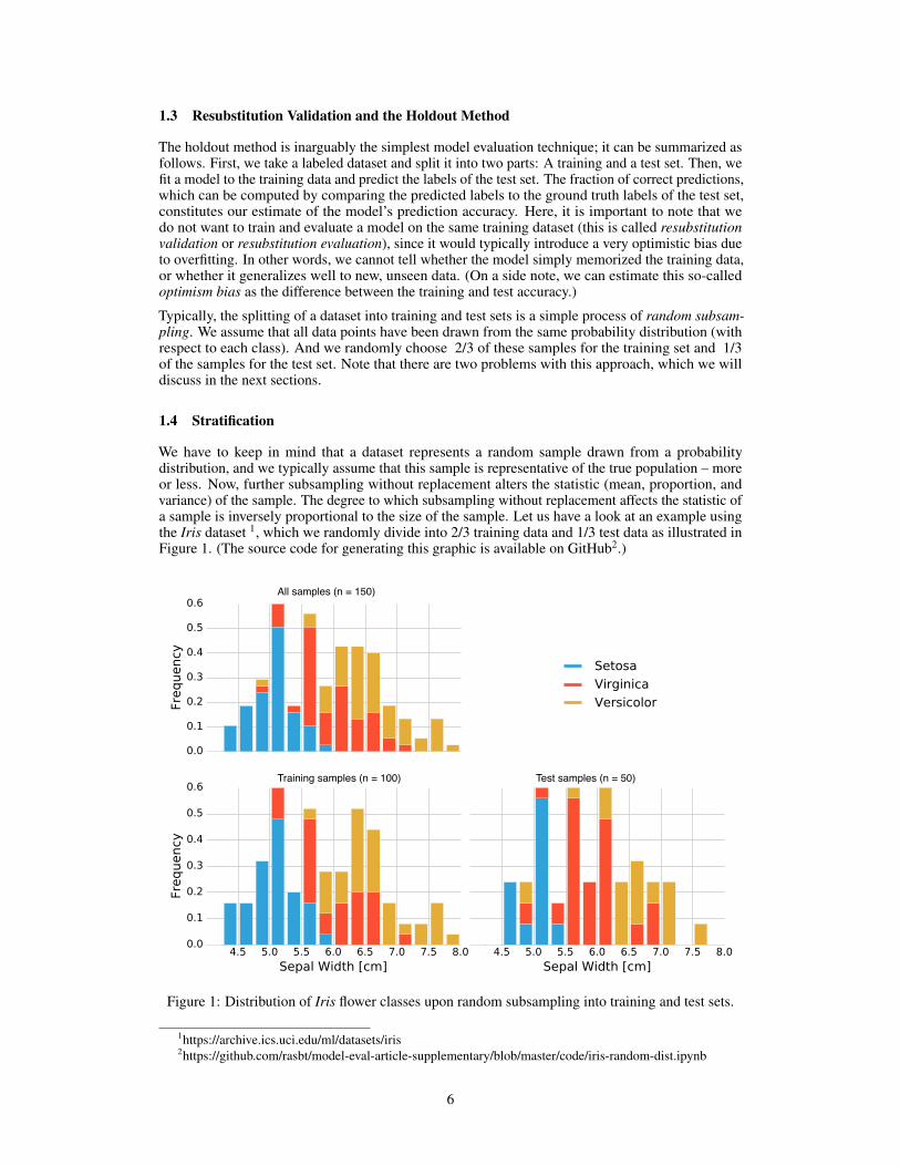
We have to keep in mind that a dataset represents a random sample drawn from a probabilitydistribution, and we typically assume that this sample is representative of the true population – moreor less. Now, further subsampling without replacement alters the statistic (mean, proportion, andvariance) of the sample. The degree to which subsampling without replacement affects the statistic ofa sample is inversely proportional to the size of the sample. Let us have a look at an example usingthe Iris dataset 1, which we randomly divide into 2/3 training data and 1/3 test data as illustrated inFigure 1. (The source code for generating this graphic is available on GitHub2.)

All samples (n = 150)

Training samples (n = 100) Test samples (n = 50)

Figure 1: Distribution of Iris flower classes upon random subsampling into training and test sets.

1https://archive.ics.uci.edu/ml/datasets/iris2https://github.com/rasbt/model-eval-article-supplementary/blob/master/code/iris-random-dist.ipynb

6

When we randomly divide a labeled dataset into training and test sets, we violate the assumptionof statistical independence. The Iris datasets consists of 50 Setosa, 50 Versicolor, and 50 Virginicaflowers; the flower species are distributed uniformly:

• 33.3% Setosa• 33.3% Versicolor• 33.3% Virginica

If a random function assigns 2/3 of the flowers (100) to the training set and 1/3 of the flowers (50) tothe test set, it may yield the following (also shown in Figure 1):

• training set→ 38 × Setosa, 28 × Versicolor, 34 × Virginica• test set→ 12 × Setosa, 22 × Versicolor, 16 × Virginica

Assuming that the Iris dataset is representative of the true population (for instance, assuming thatiris flower species are distributed uniformly in nature), we just created two imbalanced datasets withnon-uniform class distributions. The class ratio that the learning algorithm uses to learn the modelis "38% / 28% / 34%." The test dataset that is used for evaluating the model is imbalanced as well,and even worse, it is balanced in the "opposite" direction: "24% / 44% / 32%." Unless the learningalgorithm is completely insensitive to these perturbations, this is certainly not ideal. The problembecomes even worse if a dataset has a high class imbalance upfront, prior to the random subsampling.In the worst-case scenario, the test set may not contain any instance of a minority class at all. Thus,a recommended practice is to divide the dataset in a stratified fashion. Here, stratification simplymeans that we randomly split a dataset such that each class is correctly represented in the resultingsubsets (the training and the test set) – in other words, stratification is an approach to maintain theoriginal class proportion in resulting subsets.

It shall be noted that random subsampling in non-stratified fashion is usually not a big concern whenworking with relatively large and balanced datasets. However, in my opinion, stratified resampling isusually beneficial in machine learning applications. Moreover, stratified sampling is incredibly easyto implement, and Ron Kohavi provides empirical evidence [Kohavi, 1995] that stratification has apositive effect on the variance and bias of the estimate in k-fold cross-validation, a technique that willbe discussed later in this article.

1.5 Holdout Validation

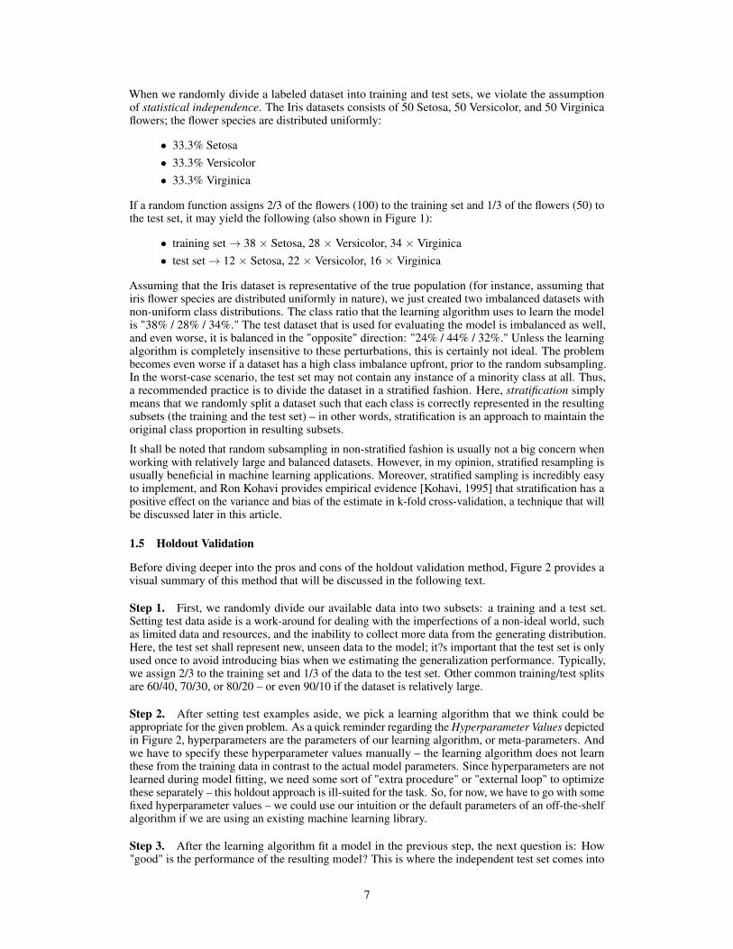
Before diving deeper into the pros and cons of the holdout validation method, Figure 2 provides avisual summary of this method that will be discussed in the following text.

Step 1. First, we randomly divide our available data into two subsets: a training and a test set.Setting test data aside is a work-around for dealing with the imperfections of a non-ideal world, suchas limited data and resources, and the inability to collect more data from the generating distribution.Here, the test set shall represent new, unseen data to the model; it?s important that the test set is onlyused once to avoid introducing bias when we estimating the generalization performance. Typically,we assign 2/3 to the training set and 1/3 of the data to the test set. Other common training/test splitsare 60/40, 70/30, or 80/20 – or even 90/10 if the dataset is relatively large.

Step 2. After setting test examples aside, we pick a learning algorithm that we think could beappropriate for the given problem. As a quick reminder regarding the Hyperparameter Values depictedin Figure 2, hyperparameters are the parameters of our learning algorithm, or meta-parameters. Andwe have to specify these hyperparameter values manually – the learning algorithm does not learnthese from the training data in contrast to the actual model parameters. Since hyperparameters are notlearned during model fitting, we need some sort of "extra procedure" or "external loop" to optimizethese separately – this holdout approach is ill-suited for the task. So, for now, we have to go with somefixed hyperparameter values – we could use our intuition or the default parameters of an off-the-shelfalgorithm if we are using an existing machine learning library.

Step 3. After the learning algorithm fit a model in the previous step, the next question is: How"good" is the performance of the resulting model? This is where the independent test set comes into

7

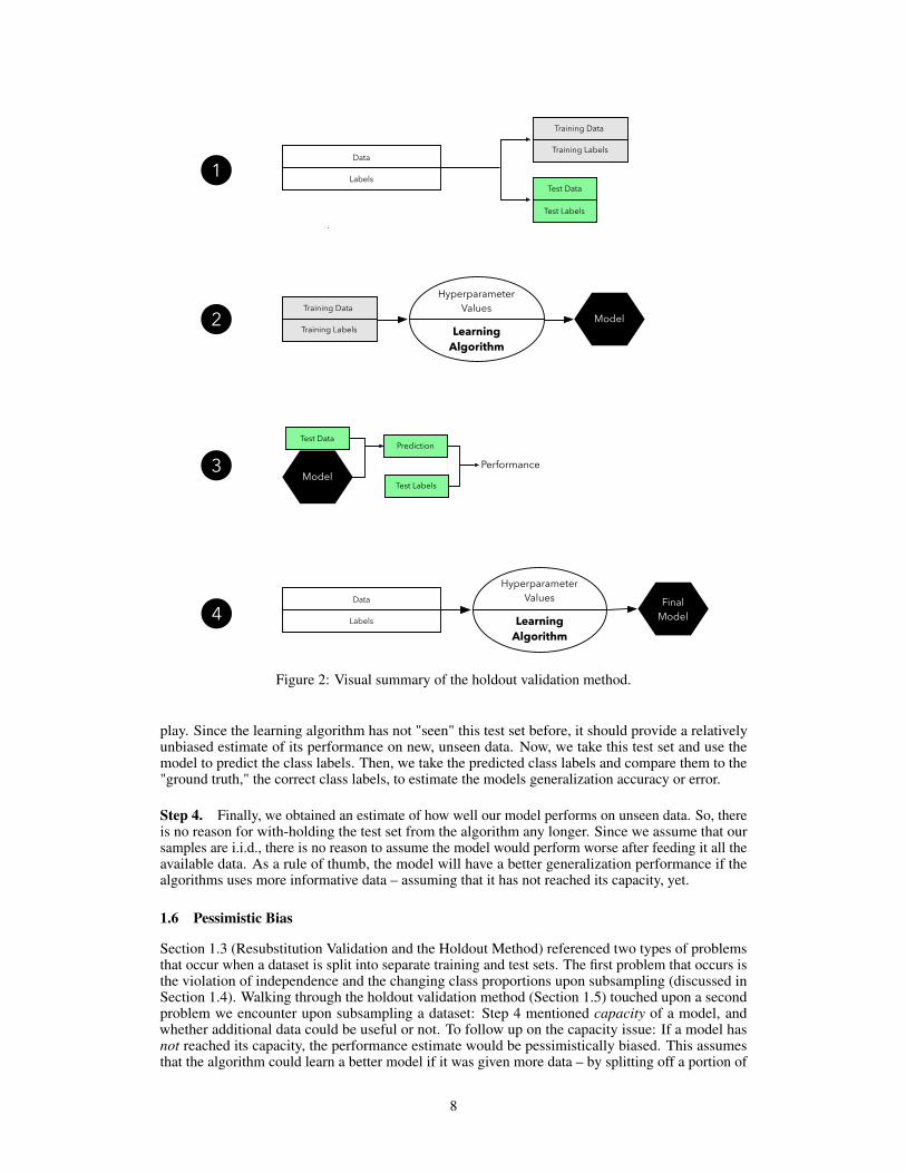
Learning Algorithm

Hyperparameter Values

Model

Prediction

Test Labels

PerformanceModel

Learning Algorithm

Hyperparameter Values Final

Model

2

3

4

1

Test Labels

Test Data

Training Data

Training LabelsData

Labels

Data

Labels

Training Data

Training Labels

Test Data

Figure 2: Visual summary of the holdout validation method.

play. Since the learning algorithm has not "seen" this test set before, it should provide a relativelyunbiased estimate of its performance on new, unseen data. Now, we take this test set and use themodel to predict the class labels. Then, we take the predicted class labels and compare them to the"ground truth," the correct class labels, to estimate the models generalization accuracy or error.

Step 4. Finally, we obtained an estimate of how well our model performs on unseen data. So, thereis no reason for with-holding the test set from the algorithm any longer. Since we assume that oursamples are i.i.d., there is no reason to assume the model would perform worse after feeding it all theavailable data. As a rule of thumb, the model will have a better generalization performance if thealgorithms uses more informative data – assuming that it has not reached its capacity, yet.

1.6 Pessimistic Bias

Section 1.3 (Resubstitution Validation and the Holdout Method) referenced two types of problemsthat occur when a dataset is split into separate training and test sets. The first problem that occurs isthe violation of independence and the changing class proportions upon subsampling (discussed inSection 1.4). Walking through the holdout validation method (Section 1.5) touched upon a secondproblem we encounter upon subsampling a dataset: Step 4 mentioned capacity of a model, andwhether additional data could be useful or not. To follow up on the capacity issue: If a model hasnot reached its capacity, the performance estimate would be pessimistically biased. This assumesthat the algorithm could learn a better model if it was given more data – by splitting off a portion of

8

the dataset for testing, we withhold valuable data for estimating the generalization performance (forinstance, the test dataset). To address this issue, one might fit the model to the whole dataset afterestimating the generalization performance (see Figure 2 step 4). However, using this approach, wecannot estimate its generalization performance of the refit model, since we have now "burned" thetest dataset. It?s a dilemma that we cannot really avoid in real-world application, but we should beaware that our estimate of the generalization performance may be pessimistically biased if only aportion of the dataset, the training dataset, is used for model fitting (this is especially affects modelsfit to relatively small datasets).

1.7 Confidence Intervals via Normal Approximation

Using the holdout method as described in Section 1.5, we computed a point estimate of the gener-alization performance of a model. Certainly, a confidence interval around this estimate would notonly be more informative and desirable in certain applications, but our point estimate could be quitesensitive to the particular training/test split (for instance, suffering from high variance). A simpleapproach for computing confidence intervals of the predictive accuracy or error of a model is via theso-called normal approximation. Here, we assume that the predictions follow a normal distribution,to compute the confidence interval on the mean on a single training-test split under the central limittheorem. The following text illustrates how this works.

As discussed earlier, we compute the prediction accuracy as follows:

ACCS =1

n

n∑i=1

δ(L(yi, yi)), (10)

where L(·) is the 0-1 loss function (Equation 3), and n denotes the number of samples in the testdataset. Further, let yi be the predicted class label and yi be the ground truth class label of the ith testexample, respectively. So, we could now consider each prediction as a Bernoulli trial, and the numberof correct predictions X is following a binomial distribution X ∼ (n, p) with n test examples, ktrials, and the probability of success p, where n ∈ N and p ∈ [0, 1] :

f(k;n, p) = Pr(X = k) =

(n

k

)pk(1− p)n−k, (11)

for k = 0, 1, 2, ..., n, where

(n

k

)=

n!

k!(n− k)!. (12)

(Here, p is the probability of success, and consequently, (1− p) is the probability of failure – a wrongprediction.)

Now, the expected number of successes is computed as µ = np, or more concretely, if the model hasa 50% success rate, we expect 20 out of 40 predictions to be correct. The estimate has a variance of

σ2 = np(1− p) = 10 (13)

and a standard deviation of

σ =√np(1− p) = 3.16. (14)

Since we are interested in the average number of successes, not its absolute value, we compute thevariance of the accuracy estimate as

σ2 =1

nACCS(1−ACCS), (15)

9

and the respective standard deviation as

σ =

√1

nACCS(1−ACCS). (16)

Under the normal approximation, we can then compute the confidence interval as

ACCS ± z√

1

nACCS (1−ACCS), (17)

where α is the error quantile and z is the 1 − α2 quantile of a standard normal distribution. For a

typical confidence interval of 95%, (α = 0.05), we have z = 1.96.

In practice, however, I would rather recommend repeating the training-test split multiple times tocompute the confidence interval on the mean estimate (for instance, averaging the individual runs).In any case, one interesting take-away for now is that having fewer samples in the test set increasesthe variance (see n in the denominator above) and thus widens the confidence interval. Confidenceintervals and estimating uncertainty will be discussed in more detail in the next section, Section 2.

2 Bootstrapping and Uncertainties

2.1 Overview

The previous section (Section 1, Introduction: Essential Model Evaluation Terms and Techniques)introduced the general ideas behind model evaluation in supervised machine learning. We discussedthe holdout method, which helps us to deal with real world limitations such as limited access to new,labeled data for model evaluation. Using the holdout method, we split our dataset into two parts: Atraining and a test set. First, we provide the training data to a supervised learning algorithm. Thelearning algorithm builds a model from the training set of labeled observations. Then, we evaluate thepredictive performance of the model on an independent test set that shall represent new, unseen data.Also, we briefly introduced the normal approximation, which requires us to make certain assumptionsthat allow us to compute confidence intervals for modeling the uncertainty of our performanceestimate based on a single test set, which we have to take with a grain of salt.

This section introduces some of the advanced techniques for model evaluation. We will start bydiscussing techniques for estimating the uncertainty of our estimated model performance as wellas the model’s variance and stability. And after getting these basics under our belt, we will look atcross-validation techniques for model selection in the next article in this series. As we remember fromSection 1, there are three related, yet different tasks or reasons why we care about model evaluation:

1. We want to estimate the generalization accuracy, the predictive performance of a model onfuture (unseen) data.

2. We want to increase the predictive performance by tweaking the learning algorithm andselecting the best-performing model from a given hypothesis space.

3. We want to identify the machine learning algorithm that is best-suited for the problem athand. Hence, we want to compare different algorithms, selecting the best-performing one aswell as the best-performing model from the algorithm’s hypothesis space.

(The code for generating the figures discussed in this section are available on GitHub3.)

3https://github.com/rasbt/model-eval-article-supplementary/blob/master/code/resampling-and-kfold.ipynb

10

2.2 Resampling

The first section of this article introduced the prediction accuracy or error measures of classificationmodels. To compute the classification error or accuracy on a dataset S, we defined the followingequation:

ERRS =1

n

n∑i=1

L(yi, yi

)= 1− ACCS . (18)

Here, L(·) represents the 0-1 loss, which is computed from a predicted class label (yi) and a trueclass label (yi) for i = 1, ..., n in dataset S:

L(yi, yi) =

0 if yi = yi

1 if yi 6= yi.

(19)

In essence, the classification error is simply the count of incorrect predictions divided by the numberof samples in the dataset. Vice versa, we compute the prediction accuracy as the number of correctpredictions divided by the number of samples.

Note that the concepts presented in this section also apply to other types of supervised learning,such as regression analysis. To use the resampling methods presented in the following sections forregression models, we swap the accuracy or error computation by, for example, the mean squarederror (MSE):

MSES =1

n

n∑i=1

(yi − yi)2. (20)

As we learned in Section 1, performance estimates may suffer from bias and variance, and we areinterested in finding a good trade-off. For instance, the resubstitution evaluation (fitting a model toa training set and using the same training set for model evaluation) is heavily optimistically biased.Vice versa, withholding a large portion of the dataset as a test set may lead to pessimistically biasedestimates. While reducing the size of the test set may decrease this pessimistic bias, the variance of aperformance estimates will most likely increase. An intuitive illustration of the relationship betweenbias and variance is given in Figure 3. This section will introduce alternative resampling methods forfinding a good balance between bias and variance for model evaluation and selection.

The reason why a proportionally large test sets increase the pessimistic bias is that the model maynot have reached its full capacity, yet. In other words, the learning algorithm could have formulateda more powerful, more generalizable hypothesis for classification if it had seen more data. Todemonstrate this effect, Figure 4 shows learning curves of a softmax classifiers, which were fitted tosmall subsets of the MNIST4 dataset.

To generate the learning curves shown in Figure 4, 500 random samples of each of the ten classesfrom MNIST – instances of the handwritten digits 0 to 9 – were drawn. The 5000-sample MNISTsubset was then randomly divided into a 3500-sample training subset and a test set containing 1500samples while keeping the class proportions intact via stratification. Finally, even smaller subsetsof the 3500-sample training set were produced via randomized, stratified splits, and these subsetswere used to fit softmax classifiers and the same 1500-sample test set was used to evaluate theirperformances (samples may overlap between these training subsets). Looking at the plot above, wecan see two distinct trends. First, the resubstitution accuracy (training set) declines as the number oftraining samples grows. Second, we observe an improving generalization accuracy (test set) withan increasing training set size. These trends can likely be attributed to a reduction in overfitting. Ifthe training set is small, the algorithm is more likely picking up noise in the training set so that themodel fails to generalize well to data that it has not seen before. This observation also explains thepessimistic bias of the holdout method: A training algorithm may benefit from more training data,

4http://yann.lecun.com/exdb/mnist

11

Low Variance(Precise)

High Variance(Not Precise)

Low

Bia

s(A

ccur

ate)

Hig

h B

ias

(Not

Acc

urat

e)

Figure 3: Illustration of bias and variance.

Figure 4: Learning curves of softmax classifiers fit to MNIST.

data that was withheld for testing. Thus, after we evaluated a model, we may want to run the learningalgorithm once again on the complete dataset before we use it in a real-world application.

Now, that we established the point of pessimistic biases for disproportionally large test sets, wemay ask whether it is a good idea to decrease the size of the test set. Decreasing the size of the testset brings up another problem: It may result in a substantial variance of our model’s performanceestimate. The reason is that it depends on which instances end up in training set, and which particularinstances end up in test set. Keeping in mind that each time we resample a dataset, we alter thestatistics of the distribution of the sample. Most supervised learning algorithms for classificationand regression as well as the performance estimates operate under the assumption that a dataset

12

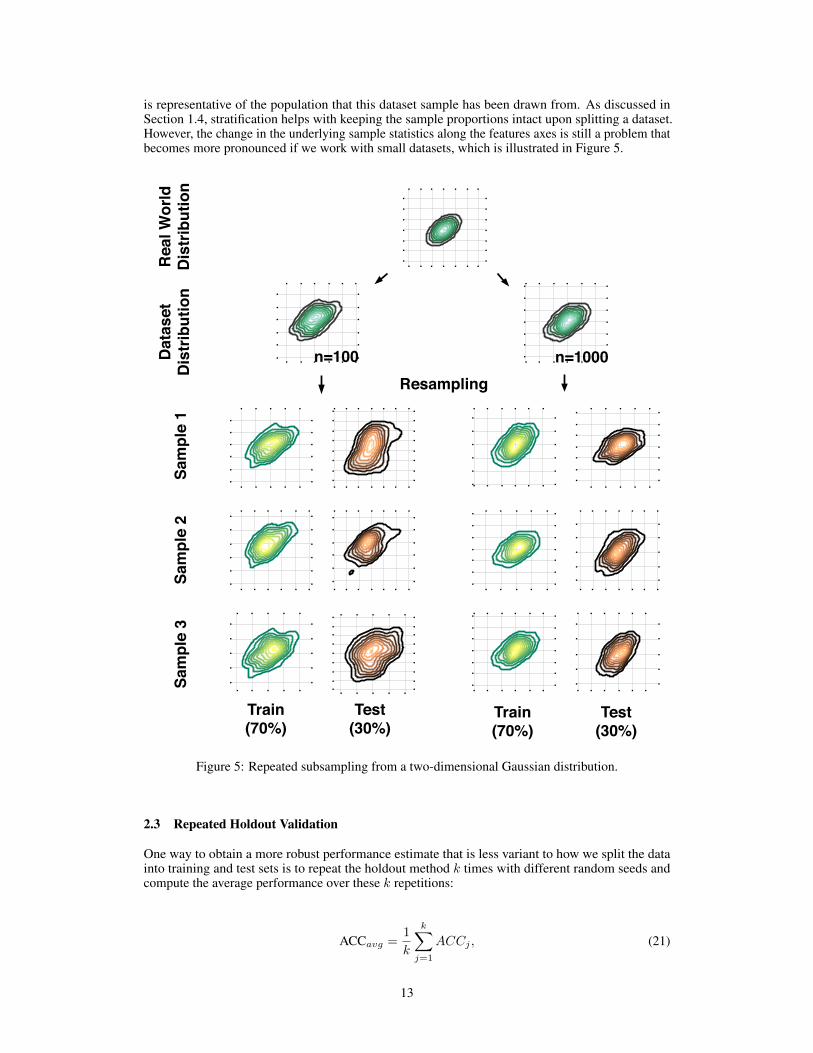
is representative of the population that this dataset sample has been drawn from. As discussed inSection 1.4, stratification helps with keeping the sample proportions intact upon splitting a dataset.However, the change in the underlying sample statistics along the features axes is still a problem thatbecomes more pronounced if we work with small datasets, which is illustrated in Figure 5.

Dat

aset

D

istr

ibut

ion

Sam

ple

1Sa

mpl

e 2

Sam

ple

3

Train(70%)

Test (30%)

Train(70%)

Test (30%)

n=1000n=100

Rea

l Wor

ld

Dis

trib

utio

n

Resampling

Figure 5: Repeated subsampling from a two-dimensional Gaussian distribution.

2.3 Repeated Holdout Validation

One way to obtain a more robust performance estimate that is less variant to how we split the datainto training and test sets is to repeat the holdout method k times with different random seeds andcompute the average performance over these k repetitions:

ACCavg =1

k

k∑j=1

ACCj , (21)

13

where ACCj is the accuracy estimate of the jth test set of size m,

ACCj = 1− 1

m

m∑i=1

L(yi, yi

). (22)

This repeated holdout procedure, sometimes also called Monte Carlo Cross-Validation, provides abetter estimate of how well our model may perform on a random test set, compared to the standardholdout validation method. Also, it provides information about the model’s stability – how the model,produced by a learning algorithm, changes with different training set splits. Figure 6 shall illustratehow repeated holdout validation may look like for different training-test split using the Iris dataset tofit to 3-nearest neighbors classifiers.

50/50 Train-Test Split Avg. Acc. 0.95

90/10 Train-Test Split Avg. Acc. 0.96

Figure 6: Repeated holdout validation with 3-nearest neighbor classifiers fit to the Iris dataset.

The left subplot in Figure 6 was generated by performing 50 stratified training/test splits with 75samples in the test and training set each; a 3-nearest neighbors model was fit to the training set andevaluated on the test set in each repetition. The average accuracy of these 50 50/50 splits was 95%.The same procedure was used to produce the right subplot in Figure 6. Here, the test sets consisted ofonly 15 samples each due to the 90/10 splits, and the average accuracy over these 50 splits was 96%.Figure 6 demonstrates two of the points that were previously discussed. First, we see that the varianceof our estimate increases as the size of the test set decreases. Second, we see a small increase in thepessimistic bias when we decrease the size of the training set – we withhold more training data in the50/50 split, which may be the reason why the average performance over the 50 splits is slightly lowercompared to the 90/10 splits.

The next section introduces an alternative method for evaluating a model?s performance; it willdiscuss about different flavors of the bootstrap method that are commonly used to infer the uncertaintyof a performance estimate.

2.4 The Bootstrap Method and Empirical Confidence Intervals

The previous examples of Monte Carlo Cross-Validation may have convinced us that repeated holdoutvalidation could provide us with a more robust estimate of a model’s performance on random testsets compared to an evaluation based on a single train/test split via holdout validation (Section1.5). In addition, the repeated holdout may give us an idea about the stability of our model. Thissection explores an alternative approach to model evaluation and for estimating uncertainty using thebootstrap method.

Let us assume that we would like to compute a confidence interval around a performance estimateto judge its certainty – or uncertainty. How can we achieve this if our sample has been drawnfrom an unknown distribution? Maybe we could use the sample mean as a point estimate of thepopulation mean, but how would we compute the variance or confidence intervals around the mean ifits distribution is unknown? Sure, we could collect multiple, independent samples; this is a luxury weoften do not have in real world applications, though. Now, the idea behind the bootstrap is to generate

14

"new samples" by sampling from an empirical distribution. As a side note, the term "bootstrap" likelyoriginated from the phrase "to pull oneself up by one’s bootstraps:"

Circa 1900, to pull (oneself) up by (one’s) bootstraps was used figuratively ofan impossible task (Among the "practical questions" at the end of chapter one ofSteele’s "Popular Physics" schoolbook (1888) is "Why can not a man lift himselfby pulling up on his boot-straps?". By 1916 its meaning expanded to include"better oneself by rigorous, unaided effort." The meaning "fixed sequence ofinstructions to load the operating system of a computer" (1953) is from the notionof the first-loaded program pulling itself, and the rest, up by the bootstrap.[Source: Online Etymology Dictionary5]

The bootstrap method is a resampling technique for estimating a sampling distribution, and in thecontext of this article, we are particularly interested in estimating the uncertainty of a performanceestimate – the prediction accuracy or error. The bootstrap method was introduced by Bradley Efronin 1979 [Efron, 1992]. About 15 years later, Bradley Efron and Robert Tibshirani even devoted awhole book to the bootstrap, "An Introduction to the Bootstrap" [Efron and Tibshirani, 1994], whichis a highly recommended read for everyone who is interested in more details on this topic. In brief,the idea of the bootstrap method is to generate new data from a population by repeated sampling fromthe original dataset with replacement – in contrast, the repeated holdout method can be understood assampling without replacement. Walking through it step by step, the bootstrap method works like this:

1. We are given a dataset of size n.2. For b bootstrap rounds:

We draw one single instance from this dataset and assign it to the jth bootstrap sample.We repeat this step until our bootstrap sample has size n – the size of the original dataset.Each time, we draw samples from the same original dataset such that certain examples mayappear more than once in a bootstrap sample and some not at all.

3. We fit a model to each of the b bootstrap samples and compute the resubstitution accuracy.4. We compute the model accuracy as the average over the b accuracy estimates (Equation 23).

ACCboot =1

b

b∑j=1

1

n

n∑i=1

(1− L

(yi, yi

))(23)

As discussed previously, the resubstitution accuracy usually leads to an extremely optimistic bias,since a model can be overly sensible to noise in a dataset. Originally, the bootstrap method aims todetermine the statistical properties of an estimator when the underlying distribution was unknownand additional samples are not available. So, in order to exploit this method for the evaluation ofpredictive models, such as hypotheses for classification and regression, we may prefer a slightlydifferent approach to bootstrapping using the so-called Leave-One-Out Bootstrap (LOOB) technique.Here, we use out-of-bag samples as test sets for evaluation instead of evaluating the model on thetraining data. Out-of-bag samples are the unique sets of instances that are not used for model fittingas shown in Figure 7.

Figure 7 illustrates how three random bootstrap samples drawn from an exemplary ten-sample dataset(x1, x2, ..., x10) and how the out-of-bag sample might look like. In practice, Bradley Efron andRobert Tibshirani recommend drawing 50 to 200 bootstrap samples as being sufficient for producingreliable estimates [Efron and Tibshirani, 1994].

Taking a step back, let us assume that a sample that has been drawn from a normal distribution. Usingbasic concepts from statistics, we use the sample mean x as a point estimate of the population meanµ:

x =1

n

n∑i=1

xi. (24)

5https://www.etymonline.com/word/bootstrap

15

x1

x1

x1

x1 x1x1

x2 x3 x4 x5 x6 x7 x8 x9 x10

x2

x2

x2

x2 x8x8 x10x7x3

x6 x9

x3 x8 x10x7x2x2 x9x6x6 x4x4x5

x10 x8x7x5 x4x3

x4x5x6x8 x9

Training Sets Test Sets

Bootstrap 1

Bootstrap 2

Bootstrap 3

Original Dataset

Figure 7: Illustration of training and test data splits in the Leave-One-Out Bootstrap (LOOB).

Similarly, the variance σ2 is estimated as follows:

VAR =1

n− 1

n∑i=1

(xi − x)2. (25)

Consequently, the standard error (SE) is computed as the standard deviation’s estimate (SD ≈ σ)divided by the square root of the sample size:

SE =SD√n. (26)

Using the standard error we can then compute a 95% confidence interval of the mean according to

x± z × σ√n, (27)

such that

x± t× SE, (28)

with z = 1.96 for the 95 % confidence interval. Since SD is the standard deviation of the population(σ) estimated from the sample, we have to consult a t-table to look up the actual value of t, whichdepends on the size of the sample – or the degreesoffreedom to be precise. For instance, given asample with n = 100, we find that t95 = 1.984.

Similarly, we can compute the 95% confidence interval of the bootstrap estimate starting with themean accuracy,

ACCboot =1

b

b∑i=1

ACCi, (29)

and use it to compute the standard error

SEboot =

√√√√ 1

b− 1

b∑i=1

(ACCi − ACCboot)2. (30)

16

Here, ACCi is the value of the statistic (the estimate ofACC) calculated on the ith bootstrap replicate.And the standard deviation of the values ACC1,ACC1, ...,ACCb is the estimate of the standard errorof ACC [Efron and Tibshirani, 1994].

Finally, we can then compute the confidence interval around the mean estimate as

ACCboot ± t× SEboot. (31)

Although the approach outlined above seems intuitive, what can we do if our samples do not follow anormal distribution? A more robust, yet computationally straight-forward approach is the percentilemethod as described by B. Efron [Efron, 1981]. Here, we pick the lower and upper confidence boundsas follows:

• ACClower = α1th percentile of the ACCboot distribution• ACCupper = α2th percentile of the ACCboot distribution,

where α1 = α and α2 = 1−α, and α is the degree of confidence for computing the 100× (1−2×α)confidence interval. For instance, to compute a 95% confidence interval, we pick α = 0.025 to obtainthe the 2.5th and 97.5th percentiles of the b bootstrap samples distribution as our upper and lowerconfidence bounds.

In practice, if the data is indeed (roughly) following a normal distribution, the "standard" confidenceinterval and percentile method typically agree as illustrated in the Figure 8.

� �

Figure 8: Comparison of the standard and percentile method for computing confidence intervalsfrom leave-one-out bootstrap samples. Subpanel A evaluates 3-nearest neighbors models on Iris, andsublpanel B shows the results of softmax regression models on MNIST.

In 1983, Bradley Efron described the .632 Estimate, a further improvement to address the pessimisticbias of the bootstrap cross-validation approach described above [Efron, 1983]. The pessimistic biasin the "classic" bootstrap method can be attributed to the fact that the bootstrap samples only containapproximately 63.2% of the unique examples from the original dataset. For instance, we can computethe probability that a given example from a dataset of size n is not drawn as a bootstrap sample asfollows:

P (not chosen) =

(1− 1

n

)n, (32)

which is asymptotically equivalent to 1e ≈ 0.368 as n→∞.

Vice versa, we can then compute the probability that a sample is chosen as

P (chosen) = 1−(

1− 1

n

)n≈ 0.632 (33)

for reasonably large datasets, so that we select approximately 0.632×n unique examples as bootstraptraining sets and reserve 0.382 × n out-of-bag examples for testing in each iteration, which isillustrated in Figure 9.

17

Figure 9: Probability of including an example from the dataset in a bootstrap sample for differentdataset sizes n.

Now, to address the bias that is due to this the sampling with replacement, Bradley Efron proposedthe .632 Estimate mentioned earlier, which is computed via the following equation:

ACCboot =1

b

b∑i=1

(0.632 · ACCh,i + 0.368 · ACCr,i

), (34)

where ACCr, i is the resubstitution accuracy, and ACCh, i is the accuracy on the out-of-bag sample.Now, while the .632 Boostrap attempts to address the pessimistic bias of the estimate, an optimisticbias may occur with models that tend to overfit so that Bradley Efron and Robert Tibshirani proposedThe .632+ Bootstrap Method [Efron and Tibshirani, 1997]. Instead of using a fixed weight ω = 0.632in

ACCboot =1

b

b∑i=1

(ω · ACCh,i + (1− ω) · ACCr,i

), (35)

we compute the weight ω as

ω =0.632

1− 0.368×R, (36)

where R is the relative overfitting rate:

R =(−1)× (ACCh,i − ACCr,i)

γ − (1− ACCh,i). (37)

(Since we are plugging ω into Equation 35 for computing ACCboot that we defined above, ACCh,iand ACCr,i still refer to the resubstitution and out-of-bag accuracy estimates in the ith bootstrapround, respectively.)

18

Further, we need to determine the no-information rate γ in order to compute R. For instance, we cancompute γ by fitting a model to a dataset that contains all possible combinations between samples x′iand target class labels yi – we pretend that the observations and class labels are independent:

γ =1

n2

n∑i=1

n∑i′=1

L(yi, f(xi′)). (38)

Alternatively, we can estimate the no-information rate γ as follows:

γ =

K∑k=1

pk(1− qk), (39)

where pk is the proportion of class k examples observed in the dataset, and qk is the proportion ofclass k examples that the classifier predicts in the dataset.

This Section continued the discussion around biases and variances in evaluating machine learningmodels in more detail. Further, it introduced the repeated hold-out method that may provide us withsome further insights into a model’s stability. Then, we looked at the bootstrap method; a techniqueborrowed from the field of statistics. We explored different flavors of this bootstrap method thathelp us estimate the uncertainty of our performance estimates. After covering the basics of modelevaluation in this and the previous section, the next section introduces hyperparameter tuning andmodel selection.

3 Cross-validation and Hyperparameter Optimization

3.1 Overview

Almost every machine learning algorithm comes with a large number of settings that we, themachine learning researchers and practitioners, need to specify. These tuning knobs, the so-calledhyperparameters, help us control the behavior of machine learning algorithms when optimizingfor performance, finding the right balance between bias and variance. Hyperparameter tuning forperformance optimization is an art in itself, and there are no hard-and-fast rules that guarantee bestperformance on a given dataset. The previous sections covered holdout and bootstrap techniques forestimating the generalization performance of a model. The e bias-variance trade-off was introducedas well as methods for computing the uncertainty of performance estimates. This third sectionfocusses on different methods of cross-validation for model evaluation and model selection. It coverscross-validation techniques to rank models from several hyperparameter configurations and estimatehow well these generalize to independent datasets.

(The code for generating the figures discussed in this section are available on GitHub6.)

3.2 About Hyperparameters and Model Selection

Previously, the holdout method and different flavors of the bootstrap were introduced to estimatethe generalization performance of our predictive models. We split the dataset into two parts: atraining and a test dataset. After the machine learning algorithm fit a model to the training set, weevaluated it on the independent test set that we withheld from the machine learning algorithm duringmodel fitting. While we were discussing challenges such as the bias-variance trade-off, we usedfixed hyperparameter settings in our learning algorithms, such as the number of k in the k-nearestneighbors algorithm. We defined hyperparameters as the parameters of the learning algorithm itself,which we have to specify a priori – before model fitting. In contrast, we referred to the parameters ofour resulting model as the model parameters.

So, what are hyperparameters, exactly? Considering the k-nearest neighbors algorithm, one exampleof a hyperparameter is the integer value of k (Figure 10). If we set k=3, the k-nearest neighborsalgorithm will predict a class label based on a majority vote among the 3-nearest neighbors in the

6https://github.com/rasbt/model-eval-article-supplementary/blob/master/code/resampling-and-kfold.ipynb

19

training set. The distance metric for finding these nearest neighbors is yet another hyperparameter ofthis algorithm.

?

k = 5

k = 3

k = 1

feature 1

feat

ure

2

Figure 10: Illustration of the k-nearest neighbors algorithm with different choices for k.

Now, the k-nearest neighbors algorithm may not be an ideal choice for illustrating the differencebetween hyperparameters and model parameters, since it is a azy learner and a nonparametric method.In this context, lazy learning (or instance-based learning) means that there is no training or modelfitting stage: A k-nearest neighbors model literally stores or memorizes the training data and uses itonly at prediction time. Thus, each training instance represents a parameter in the k-nearest neighborsmodel. In short, nonparametric models are models that cannot be described by a fixed number ofparameters that are being adjusted to the training set. The structure of parametric models is notdecided by the training data rather than being set a priori; nonparamtric models do not assume that thedata follows certain probability distributions unlike parametric methods (exceptions of nonparametricmethods that make such assumptions are Bayesian nonparametric methods). Hence, we may say thatnonparametric methods make fewer assumptions about the data than parametric methods.

In contrast to k-nearest neighbors, a simple example of a parametric method is logistic regression,a generalized linear model with a fixed number of model parameters: a weight coefficient for eachfeature variable in the dataset plus a bias (or intercept) unit. These weight coefficients in logisticregression, the model parameters, are updated by maximizing a log-likelihood function or minimizingthe logistic cost. For fitting a model to the training data, a hyperparameter of a logistic regressionalgorithm could be the number of iterations or passes over the training set (epochs) in gradient-basedoptimization. Another example of a hyperparameter would be the value of a regularization parametersuch as the lambda-term in L2-regularized logistic regression (Figure 11).

Changing the hyperparameter values when running a learning algorithm over a training set may resultin different models. The process of finding the best-performing model from a set of models that wereproduced by different hyperparameter settings is called model selection. The next section introducesan extension to the holdout method that is useful when carrying out this selection process.

3.3 The Three-Way Holdout Method for Hyperparameter Tuning

Section 1 provided an explanation why resubstitution validation is a bad approach for estimating ofthe generalization performance. Since we want to know how well our model generalizes to new data,

20

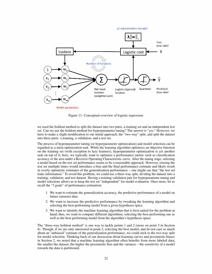
Figure 11: Conceptual overview of logistic regression.

we used the holdout method to split the dataset into two parts, a training set and an independent testset. Can we use the holdout method for hyperparameter tuning? The answer is "yes." However, wehave to make a slight modification to our initial approach, the "two-way" split, and split the datasetinto three parts: a training, a validation, and a test set.

The process of hyperparameter tuning (or hyperparameter optimization) and model selection can beregarded as a meta-optimization task. While the learning algorithm optimizes an objective functionon the training set (with exception to lazy learners), hyperparameter optimization is yet anothertask on top of it; here, we typically want to optimize a performance metric such as classificationaccuracy or the area under a Receiver Operating Characteristic curve. After the tuning stage, selectinga model based on the test set performance seems to be a reasonable approach. However, reusing thetest set multiple times would introduce a bias and the final performance estimate and likely resultin overly optimistic estimates of the generalization performance – one might say that "the test setleaks information." To avoid this problem, we could use a three-way split, dividing the dataset into atraining, validation, and test dataset. Having a training-validation pair for hyperparameter tuning andmodel selections allows us to keep the test set "independent" for model evaluation. Once more, let usrecall the "3 goals" of performance estimation:

1. We want to estimate the generalization accuracy, the predictive performance of a model onfuture (unseen) data.

2. We want to increase the predictive performance by tweaking the learning algorithm andselecting the best-performing model from a given hypothesis space.

3. We want to identify the machine learning algorithm that is best-suited for the problem athand; thus, we want to compare different algorithms, selecting the best-performing one aswell as the best-performing model from the algorithm’s hypothesis space.

The "three-way holdout method" is one way to tackle points 1 and 2 (more on point 3 in Section4). Though, if we are only interested in point 2, selecting the best model, and do not care so muchabout an "unbiased" estimate of the generalization performance, we could stick to the two-way splitfor model selection. Thinking back of our discussion about learning curves and pessimistic biasesin Section 2, we noted that a machine learning algorithm often benefits from more labeled data;the smaller the dataset, the higher the pessimistic bias and the variance – the sensitivity of a modeltowards the data is partitioned.

21

"There ain?t no such thing as a free lunch." The three-way holdout method for hyperparameter tuningand model selection is not the only – and certainly often not the best – way to approach this task. Latersections, will introduce alternative methods and discuss their advantages and trade-offs. However,before we move on to the probably most popular method for model selection, k-fold cross-validation(or sometimes also called "rotation estimation" in older literature), let us have a look at an illustrationof the 3-way split holdout method in Figure 12.

Let us walk through Figure 12 step by step.

Step 1. We start by splitting our dataset into three parts, a training set for model fitting, a validationset for model selection, and a test set for the final evaluation of the selected model.

Step 2. This step illustrates the hyperparameter tuning stage. We use the learning algorithm withdifferent hyperparameter settings (here: three) to fit models to the training data.

Step 3. Next, we evaluate the performance of our models on the validation set. This step illustratesthe model selection stage; after comparing the performance estimates, we choose the hyperparameterssettings associated with the best performance. Note that we often merge steps two and three inpractice: we fit a model and compute its performance before moving on to the next model in order toavoid keeping all fitted models in memory.

Step 4. As discussed earlier, the performance estimates may suffer from pessimistic bias if thetraining set is too small. Thus, we can merge the training and validation set after model selection anduse the best hyperparameter settings from the previous step to fit a model to this larger dataset.

Step 5. Now, we can use the independent test set to estimate the generalization performance ourmodel. Remember that the purpose of the test set is to simulate new data that the model has not seenbefore. Re-using this test set may result in an overoptimistic bias in our estimate of the model?sgeneralization performance.

Step 6. Finally, we can make use of all our data – merging training and test set– and fit a model toall data points for real-world use.

Note that fitting the model on all available data might yield a model that is likely slightly differentfrom the model evaluated in Step 5. However, in theory, using all data (that is, training and testdata) to fit the model should only improve its performance. Under this assumption, the evaluatedperformance from Step 5 might slightly underestimate the performance of the model fitted in Step6. (If we use test data for fitting, we do not have data left to evaluate the model, unless we collectnew data.) In real-world applications, having the "best possible" model is often desired – or in otherwords, we do not mind if we slightly underestimated its performance. In any case, we can regard thissixth step as optional.

3.4 Introduction to K-Fold Cross-Validation

It is about time to introduce the probably most common technique for model evaluation and modelselection in machine learning practice: k-fold cross-validation. The term cross-validation is usedloosely in literature, where practitioners and researchers sometimes refer to the train/test holdoutmethod as a cross-validation technique. However, it might make more sense to think of cross-validation as a crossing over of training and validation stages in successive rounds. Here, the mainidea behind cross-validation is that each sample in our dataset has the opportunity of being tested.K-fold cross-validation is a special case of cross-validation where we iterate over a dataset set k times.In each round, we split the dataset into k parts: one part is used for validation, and the remainingk − 1 parts are merged into a training subset for model evaluation as shown in Figure 13 , whichillustrates the process of 5-fold cross-validation.

Just as in the "two-way" holdout method (Section 1.5), we use a learning algorithm with fixedhyperparameter settings to fit models to the training folds in each iteration when we use the k-foldcross-validation method for model evaluation. In 5-fold cross-validation, this procedure will resultin five different models fitted; these models were fit to distinct yet partly overlapping training sets

22

2

1 Data

Labels

Training Data

Validation Data

Validation Labels

Test Data

Test Labels

Training Labels

PerformanceModel

Validation Data

Validation Labels

Prediction

PerformanceModel

Validation Data

Validation Labels

Prediction

PerformanceModel

Validation Data

Validation Labels

Prediction

Best Model

Learning Algorithm

Hyperparameter values

ModelHyperparameter values

Hyperparameter values

Model

Model

Training Data

Training Labels

Learning Algorithm

Best Hyperparameter

Values Final Model

6 Data

Labels

3

Best Hyperparameter

values

Prediction

Test Labels

PerformanceModel

4

Test Data

Learning Algorithm

Best Hyperparameter

ValuesModel

Training Data

Training Labels

5

Validation Data

Validation Labels

Figure 12: Illustration of the three-way holdout method for hyperparameter tuning.

and evaluated on non-overlapping validation sets. Eventually, we compute the cross-validationperformance as the arithmetic mean over the k performance estimates from the validation sets.

23

1st

2nd

3rd

4th

5th

K Ite

ratio

ns (K

-Fol

ds)

Validation Fold

Training Fold

Learning Algorithm

Hyperparameter Values

Model

Training Fold Data

Training Fold LabelsPrediction

PerformanceModel

Validation Fold Data

Validation Fold Labels

Performance

Performance

Performance

Performance

Performance

1

2

3

4

5

Performance 1 5 ∑

5

i =1Performance i=

A

B C

Figure 13: Illustration of the k-fold cross-validation procedure.

We saw the main difference between the "two-way" holdout method and k-fold cross validation:k-fold cross-validation uses all data for training and testing. The idea behind this approach is to reducethe pessimistic bias by using more training data in contrast to setting aside a relatively large portionof the dataset as test data. And in contrast to the repeated holdout method, which was discussed inSection 2, test folds in k-fold cross-validation are not overlapping. In repeated holdout, the repeateduse of samples for testing results in performance estimates that become dependent between rounds;this dependence can be problematic for statistical comparisons, which we will be discussed in Section4. Also, k-fold cross-validation guarantees that each sample is used for validation in contrast to therepeated holdout-method, where some samples may never be part of the test set.

This section introduced k-fold cross-validation for model evaluation. In practice, however, k-foldcross-validation is more commonly used for model selection or algorithm selection. K-fold cross-validation for model selection is a topic that we will be covered in the next sections, and algorithmselection will be discussed in detail throughout Section 4.

3.5 Special Cases: 2-Fold and Leave-One-Out Cross-Validation

At this point, you may wonder why k = 5 was chosen to illustrate k-fold cross-validation in theprevious section. One reason is that it makes it easier to illustrate k-fold cross-validation compactly.

24

Moreover, k = 5 is also a common choice in practice, since it is computationally less expensivecompared to larger values of k. If k is too small, though, the pessimistic bias of the performanceestimate may increase (since less training data is available for model fitting), and the variance of theestimate may increase as well since the model is more sensitive to how the data was split (in the nextsections, experiments will be discussed that suggest k = 10 as a good choice for k).

In fact, there are two prominent, special cases of k-fold cross validation: k = 2 and k = n. Mostliterature describes 2-fold cross-validation as being equal to the holdout method. However, thisstatement would only be true if we performed the holdout method by rotating the training andvalidation set in two rounds (for instance, using exactly 50% data for training and 50% of theexamples for validation in each round, swapping these sets, repeating the training and evaluationprocedure, and eventually computing the performance estimate as the arithmetic mean of the twoperformance estimates on the validation sets). Given how the holdout method is most commonlyused though, this article describes the holdout method and 2-fold cross-validation as two differentprocesses as illustrated in Figure 14.

1 2 3 4 5 6 7 8 109

1 2 3 4 5 6 7 8 109

1 2 3 4 5 6 7 8 109

1 2 3 4 5 6 7 8 109

1 2 3 4 5 6 7 8 109

...

1 2 3 4 5 6 7 8 109

1 2 3 4 5 6 7 8 109 Holdout Method

2-Fold Cross-Validation

Repeated Holdout

Training Evaluation

Figure 14: Comparison of the holdout method, 2-fold cross-validation, and the repeated holdoutmethod.

Now, if we set k = n, that is, if we set the number of folds as being equal to the number oftraining instances, we refer to the k-fold cross-validation process as Leave-One-Out Cross-Validation(LOOCV), which is illustrated in Figure 15. In each iteration during LOOCV, we fit a model to n− 1samples of the dataset and evaluate it on the single, remaining data point. Although this process iscomputationally expensive, given that we have n iterations, it can be useful for small datasets, caseswhere withholding data from the training set would be too wasteful.

Several studies compared different values of k in k-fold cross-validation, analyzing how the choice ofk affects the variance and the bias of the estimate. Unfortunately, there is no Free Lunch though asshown by Yohsua Bengio and Yves Grandvalet in "No unbiased estimator of the variance of k-foldcross-validation:"

25

1 2 3 4 5 6 7 8 109

1 2 3 4 5 6 7 8 109

1 2 3 4 5 6 7 8 109

1 2 3 4 5 6 7 8 109

1 2 3 4 5 6 7 8 109

1 2 3 4 5 6 7 8 109

1 2 3 4 5 6 7 8 109

1 2 3 4 5 6 7 8 109

1 2 3 4 5 6 7 8 109

1 2 3 4 5 6 7 8 109

Training evaluation

Figure 15: Illustration of leave-one-out cross-validation.

The main theorem shows that there exists no universal (valid under all distributions)unbiased estimator of the variance of K-fold cross-validation.[Bengio and Grandvalet, 2004]

However, we may still be interested in finding a "sweet spot," a value for k that seems to be a goodtrade-off between variance and bias in most cases, and the bias-variance trade-off discussion willbe continued in the next section. For now, let us conclude this section by looking at an interestingresearch project where Hawkins and others compared performance estimates via LOOCV to theholdout method and recommend the LOOCV over the latter – if computationally feasible:

[...] where available sample sizes are modest, holding back compounds for modeltesting is ill-advised. This fragmentation of the sample harms the calibration anddoes not give a trustworthy assessment of fit anyway. It is better to use all datafor the calibration step and check the fit by cross-validation, making sure thatthe cross-validation is carried out correctly. [...] The only motivation to rely onthe holdout sample rather than cross-validation would be if there was reason tothink the cross-validation not trustworthy – biased or highly variable. But neithertheoretical results nor the empiric results sketched here give any reason to disbelievethe cross-validation results.[Hawkins et al., 2003]

The conclusions in the previous quotation are partly based on the experiments carried out in this studyusing a 469-sample dataset, and Table 1 summarizes the findings in a comparison of different RidgeRegression models evaluated by LOOCV and the holdout method [Hawkins et al., 2003]. The firstrow corresponds to an experiment where the researchers used LOOCV to fit regression models to100-example training subsets. The reported "mean" refers to the averaged difference between the truecoefficients of determination (R2) and the coefficients obtained via LOOCV (here called q2) afterrepeating this procedure on different 100-example training sets and averaging the results. In rows2-4, the researchers used the holdout method for fitting models to the 100-example training sets, and

26

Table 1: Summary of the findings from the LOOCV vs. holdout comparison study conducted byHawkins and others [Hawkins et al., 2003]. See text for details.

Experiment Mean Standard deviationTrue R2 — q2 0.010 0.149True R2 — hold 50 0.028 0.184True R2 — hold 20 0.055 0.305True R2 — hold 10 0.123 0.504

they evaluated the performances on holdout sets of sizes 10, 20, and 50 samples. Each experimentwas repeated 75 times, and the mean column shows the average difference between the estimated R2

and the true R2 values. As we can see, the estimates obtained via LOOCV (q2) are the closest to thetrue R2 on average. The estimates obtained from the 50-example test set via the holdout method arealso passable, though. Based on these particular experiments, we may agree with the researchers’conclusion:

Taking the third of these points, if you have 150 or more compounds available,then you can certainly make a random split into 100 for calibration and 50 or morefor testing. However it is hard to see why you would want to do this.[Hawkins et al., 2003]

One reason why we may prefer the holdout method may be concerns about computational efficiency,if the dataset is sufficiently large. As a rule of thumb, we can say that the pessimistic bias and largevariance concerns are less problematic the larger the dataset. Moreover, it is not uncommon to repeatthe k-fold cross-validation procedure with different random seeds in hope to obtain a "more robust"estimate. For instance, if we repeated a 5-fold cross-validation run 100 times, we would computethe performance estimate for 500 test folds report the cross-validation performance as the arithmeticmean of these 500 folds. (Although this is commonly done in practice, we note that the test folds arenow overlapping.) However, there is no point in repeating LOOCV, since LOOCV always producesthe same splits.

3.6 K-fold Cross-Validation and the Bias-Variance Trade-off

Based on the study by Hawkins and others [Hawkins et al., 2003] discussed in Section 3.5 we mayprefer LOOCV over single train/test splits via the holdout method for small and moderately sizeddatasets. In addition, we can think of the LOOCV estimate as being approximately unbiased: thepessimistic bias of LOOCV (k = n) is intuitively lower compared k < n-fold cross-validation, sincealmost all (for instance, n− 1) training samples are available for model fitting.

While LOOCV is almost unbiased, one downside of using LOOCV over k-fold cross-validationwith k < n is the large variance of the LOOCV estimate. First, we have to note that LOOCV isdefect when using a discontinuous loss-function such as the 0-1 loss in classification or even incontinuous loss functions such as the mean-squared-error. It is said that LOOCV "[LOOCV has] highvariance because the test set only contains one sample" [Tan et al., 2005] and "[LOOCV] is highlyvariable, since it is based upon a single observation (x1, y1)" [James et al., 2013]. These statementsare certainly true if we refer to the variance between folds. Remember that if we use the 0-1 lossfunction (the prediction is either correct or not), we could consider each prediction as a Bernoullitrial, and the number of correct predictions X if following a binomial distribution X ≈ B(n, p),where n ∈ N and p ∈ [0, 1]; the variance of a binomial distribution is defined as

σ2 = np(1− p) (40)

We can estimate the variability of a statistic (here: the performance of the model) from the variabilityof that statistic between subsamples. Obviously though, the variance between folds is a poor estimateof the variance of the LOOCV estimate – the variability due to randomness in our training data. Now,when we are talking about the variance of LOOCV, we typically mean the difference in the resultsthat we would get if we repeated the resampling procedure multiple times on different data samplesfrom the underlying distribution. In this context interesting point has been made by Hastie, Tibshirani,and Friedman:

27

With k = n, the cross-validation estimator is approximately unbiased for the true(expected) prediction error, but can have high variance because the n "training sets"are so similar to one another.[Hastie et al., 2009]

Or in other words, we can attribute the high variance to the well-known fact that the mean of highlycorrelated variables has a higher variance than the mean of variables that are not highly correlated.Maybe, this can intuitively be explained by looking at the relationship between covariance (cov) andvariance (σ2):

covX,X = σ2X . (41)

or

covX,X = E[(X − µ)2

]= σ2

X (42)

if we let µ = E(X).

And the relationship between covariance covX,Y and correlation ρX,Y (X and Y are random variables)is defined as

covX,Y = ρX,Y σXσY , (43)

where

covX,Y = E[(X − µX)(Y − µY )] (44)

and

ρX,Y = E[(X − µX)(Y − µY )]/(σXσY ). (45)

The large variance that is often associated with LOOCV has also been observed in empirical studies[Kohavi, 1995].

Now that we established that LOOCV estimates are generally associated with a large variance and asmall bias, how does this method compare to k-fold cross-validation with other choices for k and thebootstrap method? Section 2 discussed the pessimistic bias of the standard bootstrap method, wherethe training set asymptotically (only) contains 0.632 of the samples from the original dataset; 2- or3-fold cross-validation has about the same problem (the .632 bootstrap that was designed to addressthis pessimistic bias issue). However, Kohavi also observed in his experiments [Kohavi, 1995] thatthe bias in bootstrap was still extremely large for certain real-world datasets (now, optimisticallybiased) compared to k-fold cross-validation. Eventually, Kohavi’s experiments on various real-worlddatasets suggest that 10-fold cross-validation offers the best trade-off between bias and variance.Furthermore, other researchers found that repeating k-fold cross-validation can increase the precisionof the estimates while still maintaining a small bias [Molinaro et al., 2005, Kim, 2009].

Before moving on to model selection in the next section, the following points shall summarize thediscussion of the bias-variance trade-off, by listing the general trends when increasing the number offolds or k:

• The bias of the performance estimator decreases (more accurate)

• The variance of the performance estimators increases (more variability)

• The computational cost increases (more iterations, larger training sets during fitting)

• Exception: decreasing the value of k in k-fold cross-validation to small values (for example,2 or 3) also increases the variance on small datasets due to random sampling effects.

28

3.7 Model Selection via K-fold Cross-Validation

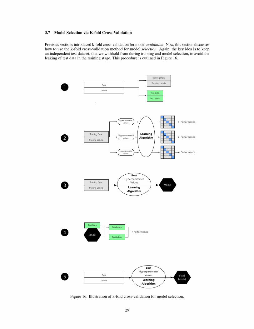
Previous sections introduced k-fold cross-validation for model evaluation. Now, this section discusseshow to use the k-fold cross-validation method for model selection. Again, the key idea is to keepan independent test dataset, that we withhold from during training and model selection, to avoid theleaking of test data in the training stage. This procedure is outlined in Figure 16.

Test Labels

Test Data

Training Data

Training LabelsData

Labels

Learning Algorithm

Hyperparameter values

Hyperparameter values

Hyperparameter values

Training Data

Training Labels

Learning Algorithm

Best Hyperparameter

ValuesModel

Training Data

Training Labels

Prediction

Test Labels

PerformanceModel

Test Data

Learning Algorithm

Best Hyperparameter

Values Final Model

Data

Labels

2

1

3

4

5

Performance

Performance

Performance

Figure 16: Illustration of k-fold cross-validation for model selection.

29

Although Figure 16 might seem complicated at first, the process is quite simple and analogous tothe "three-way holdout" workflow that we discussed at the beginning of this article. The followingparagraphs will discuss Figure 16 step by step.

Step 1. Similar to the holdout method, we split the dataset into two parts, a training and anindependent test set; we tuck away the test set for the final model evaluation step at the end (Step 4).

Step 2. In this second step, we can now experiment with various hyperparameter settings; we coulduse Bayesian optimization, randomized search, or grid search, for example. For each hyperparameterconfiguration, we apply the k-fold cross-validation method on the training set, resulting in multiplemodels and performance estimates.

Step 3. Taking the hyperparameter settings that produced the best results in the k-fold cross-validation procedure, we can then use the complete training set for model fitting with these settings.

Step 4. Now, we use the independent test set that we withheld earlier (Step 1); we use this test setto evaluate the model that we obtained from Step 3.

Step 5. Finally, after we completed the evaluation stage, we can optionally fit a model to all data(training and test datasets combined), which could be the model for (the so-called) deployment.

3.8 A Note About Model Selection and Large Datasets

When we browse the deep learning literature, we often find that that the 3-way holdout method isthe method of choice when it comes to model evaluation; it is also common in older (non-deeplearning literature) as well. As mentioned earlier, the three-way holdout may be preferred over k-foldcross-validation since the former is computationally cheap in comparison. Aside from computationalefficiency concerns, we only use deep learning algorithms when we have relatively large samplesizes anyway, scenarios where we do not have to worry about high variance – the sensitivity of ourestimates towards how we split the dataset for training, validation, and testing – so much. Thus, it isfine to use the holdout method with a training, validation, and test split over the k-fold cross-validationfor model selection if the dataset is relatively large.

3.9 A Note About Feature Selection During Model Selection

Note that if we normalize data or select features, we typically perform these operations inside thek-fold cross-validation loop in contrast to applying these steps to the whole dataset upfront beforesplitting the data into folds. Feature selection inside the cross-validation loop reduces the bias throughoverfitting, since it avoids peaking at the test data information during the training stage. However,feature selection inside the cross-validation loop may lead to an overly pessimistic estimate, sinceless data is available for training. A more detailed discussion on this topic, whether to perform featureselection inside or outside the cross-validation loop, can be found in Refaeilzadeh’s "On comparisonof feature selection algorithms" [Refaeilzadeh et al., 2007].

3.10 The Law of Parsimony

Now that we discussed model selection in the previous section, let us take a moment and consider theLaw of Parsimony, which is also known as Occam’s Razor: "Among competing hypotheses, the onewith the fewest assumptions should be selected." In model selection practice, Occam’s razor can beapplied, for example, by using the one-standard error method [Breiman et al., 1984] as follows:

1. Consider the numerically optimal estimate and its standard error.

2. Select the model whose performance is within one standard error of the value obtained instep 1.

30

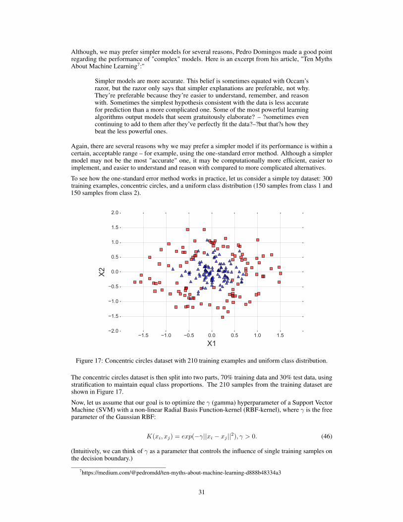
Although, we may prefer simpler models for several reasons, Pedro Domingos made a good pointregarding the performance of "complex" models. Here is an excerpt from his article, "Ten MythsAbout Machine Learning7:"

Simpler models are more accurate. This belief is sometimes equated with Occam’srazor, but the razor only says that simpler explanations are preferable, not why.They’re preferable because they’re easier to understand, remember, and reasonwith. Sometimes the simplest hypothesis consistent with the data is less accuratefor prediction than a more complicated one. Some of the most powerful learningalgorithms output models that seem gratuitously elaborate? – ?sometimes evencontinuing to add to them after they’ve perfectly fit the data?–?but that?s how theybeat the less powerful ones.

Again, there are several reasons why we may prefer a simpler model if its performance is within acertain, acceptable range – for example, using the one-standard error method. Although a simplermodel may not be the most "accurate" one, it may be computationally more efficient, easier toimplement, and easier to understand and reason with compared to more complicated alternatives.

To see how the one-standard error method works in practice, let us consider a simple toy dataset: 300training examples, concentric circles, and a uniform class distribution (150 samples from class 1 and150 samples from class 2).

Figure 17: Concentric circles dataset with 210 training examples and uniform class distribution.

The concentric circles dataset is then split into two parts, 70% training data and 30% test data, usingstratification to maintain equal class proportions. The 210 samples from the training dataset areshown in Figure 17.

Now, let us assume that our goal is to optimize the γ (gamma) hyperparameter of a Support VectorMachine (SVM) with a non-linear Radial Basis Function-kernel (RBF-kernel), where γ is the freeparameter of the Gaussian RBF:

K(xi, xj) = exp(−γ||xi − xj ||2), γ > 0. (46)

(Intuitively, we can think of γ as a parameter that controls the influence of single training samples onthe decision boundary.)

7https://medium.com/@pedromdd/ten-myths-about-machine-learning-d888b48334a3

31

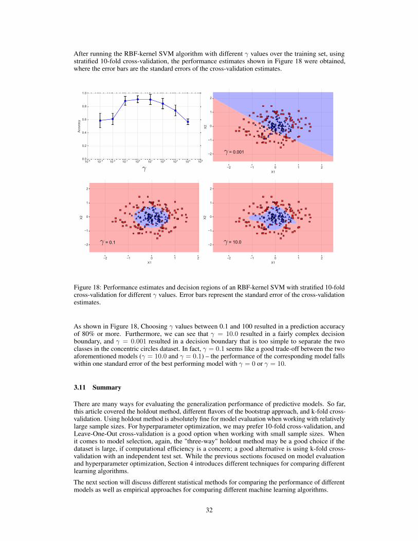
After running the RBF-kernel SVM algorithm with different γ values over the training set, usingstratified 10-fold cross-validation, the performance estimates shown in Figure 18 were obtained,where the error bars are the standard errors of the cross-validation estimates.

= 0.1

= 0.001

= 10.0

Figure 18: Performance estimates and decision regions of an RBF-kernel SVM with stratified 10-foldcross-validation for different γ values. Error bars represent the standard error of the cross-validationestimates.

As shown in Figure 18, Choosing γ values between 0.1 and 100 resulted in a prediction accuracyof 80% or more. Furthermore, we can see that γ = 10.0 resulted in a fairly complex decisionboundary, and γ = 0.001 resulted in a decision boundary that is too simple to separate the twoclasses in the concentric circles dataset. In fact, γ = 0.1 seems like a good trade-off between the twoaforementioned models (γ = 10.0 and γ = 0.1) – the performance of the corresponding model fallswithin one standard error of the best performing model with γ = 0 or γ = 10.

3.11 Summary

There are many ways for evaluating the generalization performance of predictive models. So far,this article covered the holdout method, different flavors of the bootstrap approach, and k-fold cross-validation. Using holdout method is absolutely fine for model evaluation when working with relativelylarge sample sizes. For hyperparameter optimization, we may prefer 10-fold cross-validation, andLeave-One-Out cross-validation is a good option when working with small sample sizes. Whenit comes to model selection, again, the "three-way" holdout method may be a good choice if thedataset is large, if computational efficiency is a concern; a good alternative is using k-fold cross-validation with an independent test set. While the previous sections focused on model evaluationand hyperparameter optimization, Section 4 introduces different techniques for comparing differentlearning algorithms.

The next section will discuss different statistical methods for comparing the performance of differentmodels as well as empirical approaches for comparing different machine learning algorithms.

32

4 Algorithm Comparison

[Work in progress]

References

[Bengio and Grandvalet, 2004] Bengio, Y. and Grandvalet, Y. (2004). No unbiased estimator of thevariance of k-fold cross-validation. Journal of Machine Learning Research, 5(Sep):1089–1105.

[Breiman et al., 1984] Breiman, L., Friedman, J., Stone, C. J., and Olshen, R. A. (1984). Classifica-tion and regression trees. CRC press.

[Efron, 1981] Efron, B. (1981). Nonparametric standard errors and confidence intervals. CanadianJournal of Statistics, 9(2):139–158.

[Efron, 1983] Efron, B. (1983). Estimating the error rate of a prediction rule: improvement oncross-validation. Journal of the American Statistical Association, 78(382):316–331.

[Efron, 1992] Efron, B. (1992). Bootstrap methods: another look at the jackknife. In Breakthroughsin Statistics, pages 569–593. Springer.

[Efron and Tibshirani, 1997] Efron, B. and Tibshirani, R. (1997). Improvements on cross-validation:the .632+ bootstrap method. Journal of the American Statistical Association, 92(438):548–560.

[Efron and Tibshirani, 1994] Efron, B. and Tibshirani, R. J. (1994). An introduction to the bootstrap.CRC press.

[Hastie et al., 2009] Hastie, T., Tibshirani, R., and Friedman, J. H. (2009). In The Elements ofStatistical Learning: Data Mining, Inference, and Prediction. Springer, New York.

[Hawkins et al., 2003] Hawkins, D. M., Basak, S. C., and Mills, D. (2003). Assessing model fit bycross-validation. Journal of Chemical Information and Computer Sciences, 43(2):579–586.

[James et al., 2013] James, G., Witten, D., Hastie, T., and Tibshirani, R. (2013). In An Introductionto Statistical Learning: With Applications in R. Springer, New York.

[Kim, 2009] Kim, J.-H. (2009). Estimating classification error rate: Repeated cross-validation,repeated hold-out and bootstrap. Computational Statistics & Data Analysis, 53(11):3735–3745.

[Kohavi, 1995] Kohavi, R. (1995). A study of cross-validation and bootstrap for accuracy estimationand model selection. International Joint Conference on Artificial Intelligence, 14(12):1137–1143.

[Molinaro et al., 2005] Molinaro, A. M., Simon, R., and Pfeiffer, R. M. (2005). Prediction errorestimation: a comparison of resampling methods. Bioinformatics, 21(15):3301–3307.

[Refaeilzadeh et al., 2007] Refaeilzadeh, P., Tang, L., and Liu, H. (2007). On comparison of featureselection algorithms. In Proceedings of AAAI Workshop on Evaluation Methods for MachineLearning II, pages 34–39.

[Tan et al., 2005] Tan, P.-N., Steinbach, M., and Kumar, V. (2005). In Introduction to Data Mining.Pearson Addison Wesley, Boston.

33