model fitting and methods of response : data analysis for ... · modelpittingandmethodsofresponse...
TRANSCRIPT

MODEL PITTING AND METHODS OF RESPONSEDATA ANALYSIS FOR LIQUID MIXING ON
DISTILLATION TRAYS
by
YIE-SIION WU
B.S., NATIONAL TAIWAN UNIVERSITY, TAIWAN, CHINA, I963
A MASTER'S THESIS
submitted in partial fulfillment of the
requirements for the degree
MASTER OF SCIENCE
DEPARTMENT OF CHEMICAL ENGINEERING
KANSAS STATE UNIVERSITY
Manhattan, Kansas
1968
Approved by
Major Professor

TABLE 0? CONTENTS
PageCHAPTER 1. INTRODUCTION 1
!R 2. PULSE TESTING METHOD 6
CHAPTER 3. GAMMA DISTRIBUTION MODEL 20
. ER 4. METHODS OF RESPONSE DATA ANALYSIS 49
CHAPTER 5. APPLICATION TO LIQUID MIXING ON DISTILLATION TRAYS 84
ACKNOWLEDGMENTS 100
NOTATION 101
LITERATURE CITED 105
APPENDICES - COMPUTER PROGRAMS 107
ABSTRACT

CHAPTER 1
INTRODUCTION
A chemical roaction is always coupled with physical phenomena in
a chemical process. Coupling of the transport phenomena and chemical
reactions makes the chemical process very complex to analyze and design.
Recently, considerable success has been achieved in 'systematizing the
process analysis as shown in Fig. 1-1 (1,2).
The fundamental physical variables such as flow rate, temperature,
pressure, liquid level, weir height, free area, recycle ratio, etc.,
which are directly measurable and thus can be expressed in explicit form,
are treated as the first level variables. In the classical method of
process analysis, these first level variables and chemical kinetics
are jointly analyzed, and an experimental study is carried out to verify
the results of the analysis. Actually, a process design based on such
an analysis is often very tedious, because the analysis provides incom-
plete information. The knowledge of macromixing (l,2,3), i.e. the
residence time distribution function which indicates the length of
stay of various fractions of the fluid in the vessel, should also be
a major item to be determined in the process analysis (specifically
the analysis of flow pattern). This macromixing information is, of
course, implicitly a function of the first level variables and is treated
as the second level variable. Recently, a tracer method has generally
been used to obtain the macromixing information. Today, owing to the
availability of modern high speed computers, either on-line or off-
line analysis of a process is feasible (4). For the process with

KGW
Fundamental Physical Variables L *£T
i-^
—
Flow Rate ^Temperature, Pressures Leva!
Weir .-.eight, Free Area, Rey.ux;etc,
:Variables
lFlow
i . Ul I CI I
J
Informa-
tion
wJ ^ £ — -» r— « * I «- r-v
"J IlitV. ll.Ui ik/li
2 nd1 >
Level
v;
I ( Residence Time Distribution ) jVcricblei n i
vv 3rd
~i
Micromixing Information f Level
( Degree- of Segregation ) ! Variable !
: Control lor
I
r(G<c
Informa-
tion
Chemical Kinetics
(Reaction Rate Mechanisms ')
V /
Final Conversion r
. #Products
•y* Ceneral schematic diagram tor chemise!
process analysis and feed -forward czr.wz.

first-order or decay type of kinetics, the equipment performance can
be predicted solely from the response to tracer excitation (macromixing
information) and known kinetics. For all other cases, further detail
about the fluid mixing is required. Additional information concerning
the point to point action of the fluid is the knowledge of micromixing
(l,2,3), and as may be expected, it requires much more effort to measure
than the macromixing. It is treated as the third level variable.
Though the experimental measurement of micromixing is very difficult
as compared to the measurement of macromixing, it can be shown how
bounds can be put on the micromixing (2,3) > which are the two extremes
of complete segregation and maximum mixedness, without knowing exact
details. These bounds are often narrow enough so that prediction and
design methods based on the macromixing information prove to be practical.
The micromixing is only important for processes accompanying high order,
nonlinear reactions.
In other words, the flow pattern and the kinetics are the essential
information required to predict the performance of process equipment.
The step by step information analysis of the process variables and the
correlation among them give rise to the so—called performance equations
which are required in the design and optimization of the system.
The research described herein is concerned with the first and
second level variables. The investigation emphasizes analysis of the
dynamic characteristics of a system in which fluid mixing takes place.
The general approach is as follows:
1. Select the system to be studied.
2. Select the tracer to be used.

4
3. Carry out the experimental work.
4. Select a physical model or mathematical model (or models)
to describe the flow pattern of the system.
5. Use a suitable method to analyze the response data.
Since the design of a distillation column is very important in
many industries, the understanding of fluid mixing on distillation
trays is essential. An extensive experimental system was carried out
by Johnson (5) to study the characteristics of liquid mixing on distilla-
tion trays. This work emphasizes the selection of methods in analyzing
experimental data for the purpose of fitting a model to the data.
Chapter 2 is devoted to describing the general pulse testing method,
which has been proved to be practical in determining the dynamic behavior
of a system. Various questions such as selection of a tracer, the
pulse height and width, and the detection and recording systems will
also be discussed. The notion of age distribution will be briefly
discussed and methods for the response data reduction in formulating
the transfer function of the experimental system will also be examined.
Chapter 3 is concerned with the general notion of model selection
and the description of the gamma distribution model (6). The gamma
distribution model with bypassing will be fitted to the experimental
data. The characteristics of this model will be revealed by using
several types of response curves.
Chapter 4 presents three methods of response data analysis. Each
method is followed by an example in which the model described in
Chapter 3 is used.
Chapter 5 contains the results obtained by applying the schemes
of response data analysis to the liquid mixing system on distillation
trays. The results verify the reliability of the experimental work
and the proper model selection. It is indicated that the required
computing time and the goodness of the quantitative results are major
factors which must be considered in selecting a method for analyzing
response data.
In summary, this research is concerned with the development of
what appears to be a rapid, reliable, simple procedure for procuring
knowledge of a flow pattern for liquid mixing on distillation trays.
The model selected here and the analysis method used can be applied to
other systems.

CHAPTER 2
PULSE TESTING METHOD
In dotccting tho dynamic characteristics of a system, the genoral
approach i3 to purposely excite the system (introduce a forcing distur-
bance) and to observe and analyze its response. One of the common
methods of exciting a system is the use of the sinusoidal forcing
method. The steady state response to the sinusoidal forcing is termed
the frequency response of the system. This method has many disadvan-
tages. First, the test must be sustained long enough to reach a steady
state. It is thus time consuming. Second, the oscillations may induce
unstable operation and off-specification products when the method is
directly applied to a process plant. Third, it may be difficult to
build and operate the apparatus required to induce the desired sinu-
soidal disturbance. It is thus clear that this direct method has
serious limitations as a means of obtaining dynamic data for many of
the systems in a plant operation or a laboratory study (7)» The impulse
response and the step response methods have also been used widely
(1,24,25).
Recently, the pulse testing method has been devised, which makes
it possible to obtain the needed information about the dynamic charac-
teristics of a system. This method employs a single pulse to excite
the system with all frequencies at once. By employing appropriate
computational techniques, the frequency response information can be
extracted from the resulting response (7)»
In studying mixing of fluid in a flow system, a tracer is injected

into the system in a pulse-manner. The response also appears as a
pulse. Both the input and output signals can be subjected to various
methods of analysis. The mixing characteristics of the system can be
extracted from the response data, which in turn can be used in construc-
ting a model of the system. It appears that the pulse test is a prac-
tical method.
Pulse testing (3)» Now consider that a certain amount of tracer M
is injected into a system containing fluid volume V, through which a
fluid flows at a steady rate of Q. Let C.(t) be the concentration in
the influent stream and C (t) be the concentration in the effluente
stream. If there is no dead space in the system, the tracer injected
will sooner or later come out in the exit stream. Thus a material
balance gives
fc.(t)Qdt = M = Jc (t)Qdt . (2-1)b
1o
e
Dividing this by Q, yields
JC (t)dt = §=,[C (t)dt . (2-2)^
}Je can see that if C.(t) and C (t) are plotted against t, the areas1 6
underneath both curves are the same. This, of course, follows the law
of conservation of mass. Nevertheless, the response, C (t), to that
of C.(t) has a characteristic distribution which depends only on the
flow pattern of the system. We can thus obtain considerable information
about the flow pattern in the system from the characteristic features
8
of C (t).e
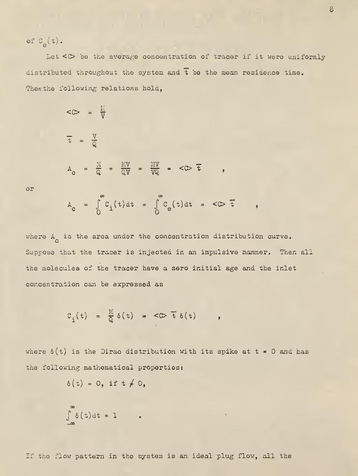
Let <0 be the average concentration of tracer if it were uniformly
distributed throughout the system and t be the mean residence time.
Then the following relations hold,
<o .. f
*- I
M MV MV ^^ r
or
c Q QV VQ
C. (t)dt =f
C (t)dt = <0 tX e
where A is the area under the concentration distribution curve.c
Suppose that the tracer is injected in an impulsive manner. Then all
the molecules of the tracer have a zero initial age and the inlet
concentration can be expressed as
Ci(t) = | 6(t) = <0 t 6(t)
where 6(t) is the Dirac distribution with its spike at t = and has
the following mathematical properties:
6(t) =0, if t / 0,
j 6(t)dt = 1
If the flow pattern in the system is an ideal plug flow, all the

molecules of the tracer spend the same period of time (mean residence
time) in the system. The exit concentration distribution is thus
given by
C (t) = $ 6(t - T) = <0 t 6(t - t) , (2-3)e m.
where 6(t - t) is the Dirac distribution with its 3pike at t = t.
If the fluid in the system is completely mixod, all the molecules of
the tracer in the system are also completely mixed throughout the system
at any instant. This in turn means that all the molecules of the tracer
in the system have an equal probability of exiting from the system. The
exi"D concentration distribution thus has the form of the exponential
decay expressed as
C (t) = <0 e"*/t
. (2-4)e
These are the ideal cases, as shown in Pig. 2-1-a. These ideal cases,
of course, seldom occur in reality. The tracer injected is usually in
an arbitrary shape and the response is also in an arbitrary shape with
a certain degree of spread, as shown in Pig. 2-1-b. The degree of
spread of the exit signal, C (t), in relation to the spread of the inlet6
signal reveals the behavior of mixing in the system (l4)»
Data normalization. In order to carry out a statistical treatment
of response data, the concentration distribution is transformed into a
probability distribution by dividing equation (2-2) by M/Q. This yields

10
C(t]
c ; Celt) Izr plug t.e.;
b: Celt) 'for compi&ts mixinglip
R.g. 2-l-a. response of en ideal system to en
impulse Uocer injection
.
Ci(t)
Mean
Time
Ce(t)
1
Decd Time
Fig. 2-1- b. Response of a nonidea! system
to en . arbitrary trace injection

11
c.(t) °° c (t)
"W dt 1 -I "W dt
•<«>
'v "
Letc At) . c (t)
x^ - -w --=-*
—
CO
and
C. (t)dt.1 x
C (t) C (t)
Y(t) - -4^T- - -=-* • (2-7)M/Qr c (t)dto
e
Then
fX(t)dt = 1 = j Y(t)dt . (2-8)
The functions, X(t) and Y(t), so obtained are the probability density
functions associated with the inlet stream and the exit stream respec-
tively. X(t)dt is the fraction of tracer in the inlet stream which
enters the system between time t and t+dt, while Y(t)dt is the fraction
of the tracer in the outlet stream which leaves the system between time
v and t+dt. Response data are usually analyzed by using the probability
distribution instead of using the concentration distribution, because
of its convenience. If Y(t) is the impulse response, it corresponds
to the so-called residence time distribution (RTD) which characterizes
the macromixing in the system. The exit age distribution is a different
name for the same function as RTD (2,3).
The scheme for measuring signals for an experimental system is
shown in Fig. 2-2-a. Both the inlet and outlet concentration signals

12
are transformed into the electrical signals in the final recording.
To assure the identity of the information of RTD, the final recording
must hold a linear relationship with respect to the concentration
throughout the detecting range. Otherwise, difficulties arise out of
the final data correction. Let X. be the proportionality factor for
the input signal recording, R. ( t) , and X be the proportionality factor
for the output signal recording, R (t). Then
R.(t) = X.C.(t)
and
R (t) = X C (t)e y e e
The block diagrams for both input and output signal transformations
are shown in Fig. 2-2-b and Pig. 2-2-c respectively. Generally, X.
and X are nearly the same but it is not always so. Frequently the
output pulse decays very slowly. It is thus better to amplify X a6
little higher than X. in order to reduce the noise effect. The area° i
under R.'(t) is now equal to
X . M <» °°
-4- =.)
R.(t)dt = J X C (t)dt , (2-9)<*
while the area under R (t) is equal to
K M • °°
-|- = P R (t)dt = P X C (t)dt . (2-10)
Dividing equation (2-9) by K.M/Q yields

13
»w
Detector *H Transducer
C (f)>< Detector
i H Transducer
L
-><
* R;Ct)
2 -Chen:-;..
r kocorucr
Fun
Fig. 2-2-a. General scheme -of instrumenvc/icri
.
R,lt)
ig. 2-2-b.,Block diagram for input signal
ce (t)K,
Re Ct)
Fig.2-2-c. Block diagram for output signal.
14
i.e.
« R. (t) » C. (t)
= P Tr^rrr^ dt = F2
. in dt
R (t) R (t)
x^ - Oi7q "•
(2-n)1
J R. (t)dt
Dividing equation (2-10) "by K M/Q yields
« R (t) » C (t)
1" ! FM75 dt
"I,
-Wft-dt
i.e.R (t) R (t)
Y^ rm --=-*— •
(2~12)e
J R (t)dte
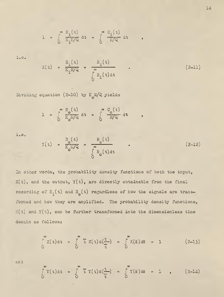
In other words, the probability density functions of both the input,
X(t), and the output, Y(t), are directly obtainable from the final
recording of R.(t) and R (t) regardless of how the signals are trans-
formed and how they are amplified. The probability density functions,
X(t) and Y(t), can be further transformed into the dimensionless time
domain as follows:
' X(t)dt =f t X(t)d(~) = J X(8)d9 = 1 (2-13)
o b toand
' Y(t)dt = f t Y(t)d(^-) = J Y(e)d6 = 1 , (2-14)*6 b t b

15
where
4-
8 = —^- = dimensionless time;
t
x(e) = tx(t) j y(e) = tY(t)
These notations will he used consistently throughout this -writing.
Mathematical treatmont. Once the probability density functions of
X(t) and Y(t) have been obtained, they can be treated further mathe-
matically.
The kth moment of the exit age distribution, Y(t), is defined
as (15)
mtyk
= I A(t)dt , k = 1,2,3 . . . (2-15)
where the subscript tyk in m . refers to the kth moment of Y(t) in
the time domain. When k = 1, the resulting expression gives the mean
of Y(t) or the first moment of Y(t), i.e.
^ty= m
tyl=
J"tY^) dt
' • ( 2-16 )
The second moment about the mean, jj, , commonly called the variance,
2o\ , is defined asty'
aty
"{(t-^yJ^t)^
raty2 " »ty (2"17)
where
mty2
=I t^(t)dt

16
Likevrice, the third moment about the mean, p, , commonly called the
skewness, a. , is defined asty'
oi =f (t - ^ + )
3 Y(t)dtty £ ^ty'
«m ~ **"% - *\, '(2"18)
where00
mty3
-.,A ( t)dt
3y the same method, the kth moment of the inlet age distribution,
X(t), is defined as
mtxk
=J"
tkX(t)dt , k = 1,2,3 . . . (2-19)
The mean of X(t) is defined as
tx-
»txl' - {«<*>" • (2-20)
The variance of X( t) is defined as
2 f /. n2„tx " I (*-**,) X^ dt
where
"tx2 ' J
Q* X < t)dt

17
The skewness of X(t) is defined as
ffj, - J (t - p. +Y )
3x(t)dto "
tx'
.2 ..3= ffitx3-^txatx-^tx' '
t 2-22 ^
wnere
m, , = f t3X(t)dt
tx3 £
The difference between the means is defined as
a^tyx **-"*, '
( 2"23 >
:he difference between the variances as
Ac? = a2 - a
2, (2-24)
tyx ty tx ' \ -r/
and the difference between the skewnesses as
Lo] = o\ - cj . (2-25)tyx ty tx v "
2 3Values of Au,^ , Ac, and Ac, are dependent on the structure
tyx 7 tyx tyx
and operating condition of the system. If they are correlated to the
model parameters of the system, this gives rise to the so-called moments
method of analysis. In general, the information of n+1 moments are
required for fitting of an n-parameter model to experimental data.
In another method of correlating response data to the model para-
meters, the Laplace transform is applied to both Y(t) and X( t) . By
taking the ratio of the transformed response gives

13
00
-StJ e"
StY(t)dt
H(s) = V- , (2-26)
fe~
StX(t)dt
which is the system transfer function in the s-domain. The s-plane
analysis fits this experimental transfer function to that of the model.
If a Fourier transformation is applied to both Y(t) and X(t), the
transfer function in the frequency domain,
J.-*»* Y(t)d1i
H(jco) = 2-, (2-27)
fe"* * X(t)dt
can be obtained. Since both Y(t) and X(t) are continuous functions
of a bounded variation which return to their initial values after a
finite time and remain so as time progresses, the integrals exist and
they may be evaluated for each value of uu. We then obtain the amplitude
ratio and phase angle from H(jou). Theoretically, they are identical
to those obtained by directly analyzing the response to the sinusoidal
forcing signal of the tracer. In other words, fitting this experimental
transfer function to that of the model is equivalent to the frequency
response analysis.
Tracer injection. Tracors such as radioisotopes, dyostuffc and
salt solutions are generally used. A tracer which is harmful to the
human body is of course not suitable for use in the food industry.
Some chemical processes may be conducted at high temperatures and high
pressures. A tracer which is evaporated or destroyed during testing
ic of coutlio not adopted; otherwise, the exit age distribution will

19
be meaningless. The general requirements for the tracer are that it
should be stable (does not react with the main stream) and easily be
detected. The moat interesting question is the optimum pulse shape
for the input. Ideally, it appears that the smaller the magnitude of
the input pulse the better. Ho -
.. over, the presence of noise necessitates
producing a response which is discernible from the interference. To
reduce the uncertainty, an increase in the pulse height is suggested
(but not exceeding the response capacity of the system). If the width
of the input is long compared with the response, the dynamics of the
system are only moderately excited; hence, high frequency responses
are suppressed, obscured, or non-existent (7). In practice, an impulse
injection function is a physical impossibility. However, the injection
time should not last too long; otherwise the high frequency response
information can not be recovered from the response data. A nearly
exact impulse injection was carried out by Williams by the arrangement
of solenoid valves and a timer (9)» Pitting of the model with experi-
mental data is then based solely on the exit response which corresponds
to the exit age distribution.

20
CHAPTER 3
GAMMA DISTRIBUTION MODEL
Constructing a model to describe mixing characteristics of a flow
system is similar to deriving a rate expression for a chemical reaction.
Although construction of a model for a flow system is tedious work, it
is essential to designing reactors for new processes and improving
performances of existing reactors. It is desirable to establish a
fairly general model which is applicable to a variety of systems rather
than to derive specific models for individual systems separately.
Elements such as plug flow, backmix flow, dead space, bypass flow,
recycle flow, cross flow, etc. are taken into consideration for con-
structing a general model. The general model then contains a number
of parameters which make it flexible in fitting it to a wide variety
of situations. However, the complexity of the accompanying mathematics
may give rise to difficulties in the fitting procedure. Furthermore,
it is possible that more than one set of parameters fit the experimental
data equally well.' This may make the model very unrealistic and unable
to represent reality. To obtain the best flexibility, simplicity and
reliability, we should construct the simplest model which closely
represents reality and whose various flow regions resemble those of
the real system (19).
An optimum way may be to subgroup the similar systems and describe
these subgroups by suitable individual models. This way, a model will
have a simple form and yet it ca.n describe the mixing characteristics
of a certain number of similar systems.

21
To construct a raodol, two approaches are adopted, namely, the
model-prescribed method and the response-analysis method. In the
model-prescribed method, a model is constructed from an imaginary
physical picture of the system. It may simply be a mathematical one.
In the response-analysis method, the response of a system is examined
before any model is specified with the hope that the analysis of the
response will shed some light on the proper choice of a model. In
theory, the response-analysis approach is more reasonable than the
model-prescribed approach because the former involves less bias in the
choice of the model than the latter. Nevertheless, owing to the rather
unsatisfactory methods of analysis available at the present time, the
response-analysis approach has not been widely accepted. Cha (6) has
discussed this approach but its practical usage has 'not been established.
}amma distribution model (GDVi) . The gamma distribution model is
essentially a mathematical model. Mathematically it corresponds to
the following probability density function (6,10).
f(t) - —i— (t - D)*-1
e- (t-D>/v
( 3_1}vp r( P )
P - 1, » > t > D - 0, v>0,
where t is a continuous variable in the time domain, p, v and D are
parameters, and T denotes the gamma function defined as
CO
P-1 -Xr(p) =
IX*-
1e~
xdx

22
wovor, the paramo Lor D nay be considered tho doad (or delay) time
of the system while p may be considered as the parameter related to
the extent of fluid mixing in the direction of flow. From appearance
curves of f(t), we can see that the exit age distributions, E(t),of
some flow systems can be represented by the typical unimodal T-distri-
bution curves. For example, by letting
p - 1, D - 0,
equation (3-1) is reduced to
f(t ) . i e-Vvv
which has the same form as the exit age distribution of the completely
mixed system, i.e.
;(t) . J_ e-V *
Note that E(t) has a dimension of time . Comparing these two forms,
we can interpret v as the mean residence time of the system. As the
value of p is further increased beyond one, as shown later, the peak
of the F-distribution gradually moves from the left to the right.
Physically this means that the flow pattern gradually deviates from the
completely mixed type. In general, various physical interpretations
can be imposed on the parameters of the T-distribution model, although
it is essentially a pure mathematical model.
If the exit age distribution of a flow system is approximated by
the f-distribution as represented by equation (3-1), f(t) is equivalent

23
to the response at the exit of the system to the impulse tracer excitation
at the inlet, i.e.
f(t) = E(t) = Y(t).
The system transfer function is equivalent to the Laplace transformation
of f(t), i.e.
H (s) -f[fj-
- Y(s) « E(s) = f(s)
because X(s) = 1 for the (unit) impulse input.
The mean of f(t) can be shown to be (6)
H t= vp + D . (3-2)
If consideration is restricted to closed systems, the mean of the exit
age distribution is equal to the mean residence-time, t (2), i.e.
H t- t = I , (3-3)
and, therefore,
v"*t
" Lt - D
(3-4)
Substituting equation (3-4) into equation (3-1) and noting that the
exit age distribution of a flow system is represented by the gamma
distribution, we have
E(t) - _?*
(t - D)^1e-p(r: }
• (3-5)(t - d) p r( P )
t-D

24
If the normalized ago is used, the normalized exit age distribution of
such a system is
where
E(8) = E(t)t = *— (e-T)*-x ex-
, (3-6)(1 -t) p r( P )
t = dimensionless time,
t
t = = dimensionless dead time.
Note that E(8) is dimensionless. Taking the Laplace transform of equation
(3-6) yields the transfer function of the gamma distribution model, i.e.
H(s) = E(s) = jVi T2
1 e~TS
. (3-7)^ y v/ L(1-t)s + pj \-> i /
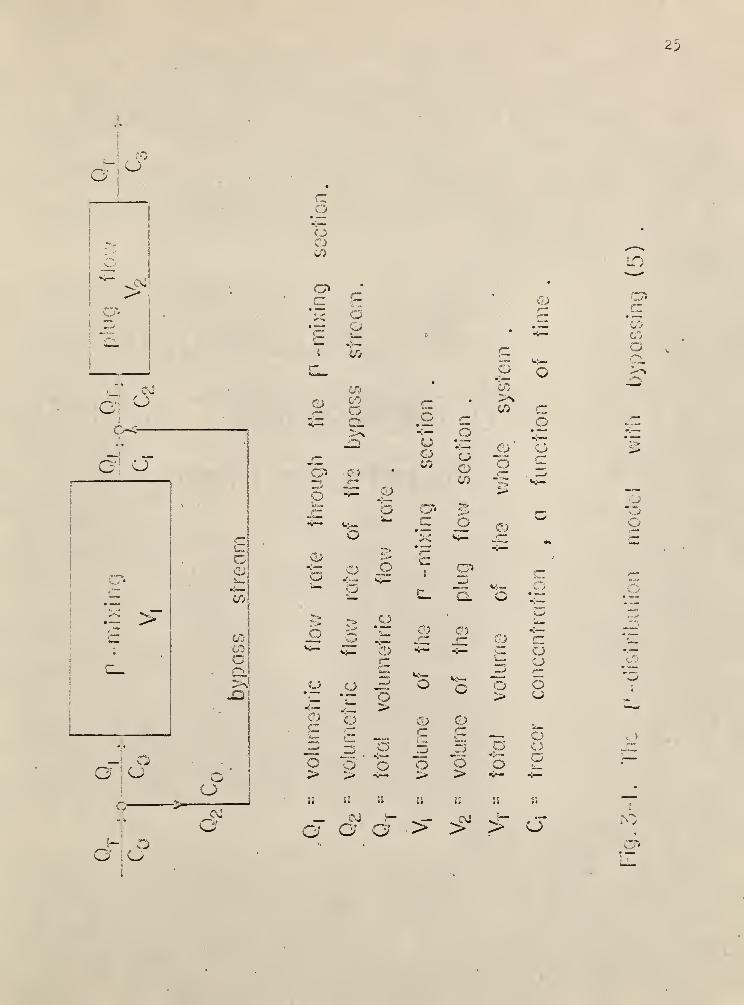
Gamma distribution model with bypassing (GDMVIB)
.
This model is a
structural modification of the original F-distribution. It is depicted
in Fig. 3-1 (5)» I"t consists of a gamma mixing section (or unit) in
series with a plug flow section. However, a portion of the inlet stream
bypasses the r-mixing unit and the by-pass stream goes directly from
the iniex of the system to the inlet pulg flow unit.
The exit age distribution, E(t)„, of the r-mixing section of the
model is then given by
E(t) r - —i—t^e-^ , (3-8)Tvp r( P )
25
O<Js
!
|
O*o—
>'
O~^
c uO
o\ u
1
.
-~N. >~I-*
1
___— o
a o
t/5
00
o
131
O
c•!—
OQiCO
<T7.•
C a<»-»
*<~ £2J
c •C'—
1 COt—**—
(/)
CO
*— CI
JQ
a
o
o o
^ > y6 V
.
—
~ "i—
O o -3'C T O
c
o
CiV
O o
11 SI SI
_ CVJ HC? w O
o
J
o
COc
o
of— cu uO* (! >
•to a
—"5
r— co
O 4— <L)
O C7>5»
o &
C- Q.
C?)
O
o
o>
*4—
o
o>
o
Cv
K—CO
CO c.2
0'
b
0*^
.2
3
Oo
ooo
^ >
LO
CI
'co-
coa
:
O
26
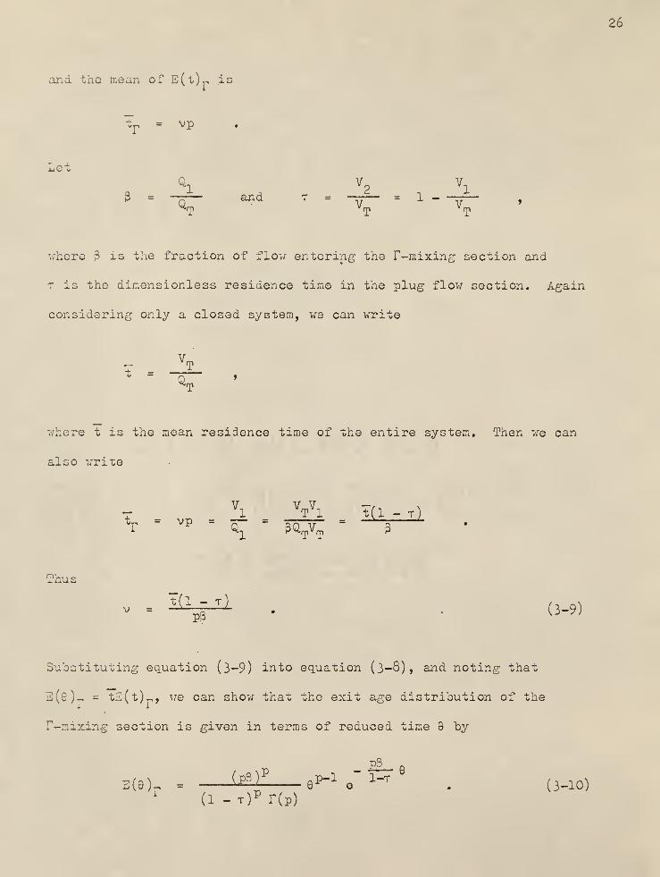
and the mean of E(t) r is
tr
= vp
LotQl
V2
Vl— and t = -y- - 1 - —
-
>
where 3 is the fraction of flow entering the T-mixing section and
t is the dimensionless residence time in the plug flow section. Again
considering only a closed system, we can write
where t is the mean residence time of the entire system. Then we can
also write
°r= vp =
qx
3QTvT
\ _Vl t(l - T )
t(l - t)V =
P3(3-9)
Substituting equation (3-9) into equation (3—8), and noting that
E(8) r = tE(t) r , we can show that the exit age distribution of the
T-mixing section is given in terms of reduced time 9 by
p pL_ e
B(e) . U&l bp-i. ^
. ( 3_10 )
(i-r) p r(p)

27
Taking the Laplaco transform of equation (3-10) gives the transfer
function for the F-mixing section, i.e.
C,(s)3
.-p
K(*k- E^r\-^r - L ( l- T )s,pp J• f««
The transfer function for the plug flow section is
9H < B>p - c^T •""
•
The material balance at the point where the bypass stream joins the
outlet stream of the r-mixing section is
C2QT
= Ql°l
+ Q2C
Dividing ^oy Q^ gives
C2
= 3CX
+ (1 - S)CQ
.
Taking the Laplace transform yields
C2(s) - 30
1(b) + (1 - &)C
q(b) . (3-13)
3y combining equations (3-11) through (3-13), it can be shown that the
transfer function of the entire system is given by
^ - ^T - V> LU-^+pg J
P
- (1 - 3)} e"TS
, (3-14)
where p, p, and t are the three parameters to be determined experimentally.
In case there is no bypassing, i.e. 3 = 1, equation (3-14) reduces to
28
equation (3-7), which is the transfer function of the T-diotribution
model. By lotting
3 = 1, p = 1, t = 0,
equation (3-14) is reduced to
H(s) =+ 1
which corresponds to the transfer function of the completely mixed
system. If
3 = o, t = l,
equation (3-14) reduces to
H(s) = e~S
which corresponds to the transfer function of the plug flow system.
Physically this means that an increase in the value of 9 tends
to emphasize the effect of mixing (F-mixing) . An increase in the value
of p tends to increase the order of the transfer function of the
r—mixing section or to reduce the effect of mixing in the axial direc-
tion. Recall that the F—mixing section is similar to a sequence of
completely mixed tanks in series but the value of p is not restricted
to an integer number (5)» An increase in the value of t tends to empahsize
the effect oz plug flow.
In summary, the three parameters play the major roles in describing
the flow pattern which generally falls between the two ideal extremes of
complete mixing and plug flow. This modified model appears to be
flexible as useful and will be used to fit Johnson's experimental data
(5). The characteristics of this model will further be revealed by

29
considering; throe typos of transient responses of the model.
. :. also response. The impulse response is the response to the
input in form of the unit impulse response,
x(e) = 6(0)
The Laplace transform of the input is
X(s) = 1
The Laplace transform of the output signal is then equal to
#Y(s) = X(s)H(s) = H(s) = E(s)
This implies that the impulse response, Y(G), of GDUWB in dimensionless
form is identical to the dimensionless exit age distribution of the
model, which can be obtained by taking the inverse transform of equation
(3-14), i.e.
Y(9) . E(6)
. P(p3)P
.
(9 . T) P-1 /^~T)
+ (1 . 3)6(e . T) ,
(i -t) p t( p )
(3-15)
The impulse responses of two typical systems, one without bypassing and
one with bypassing, are illustrated in Figs. 3-2 and 3-3.
Equation (3-15) can be reduced to that for the response of well-
known or idealized systems. For example, by letting
& = 1, t = and p = a positive integer,
equation (3-15) reduces to
Y(8) " (pfi); 91"1 °~*
. (3-16)
which corresponds to the impulse response of p - completely stirred

0.1 0.2 C.4 0.6
Fig. 3-2. Impulsi response of the. p -dl!
without bypossing.
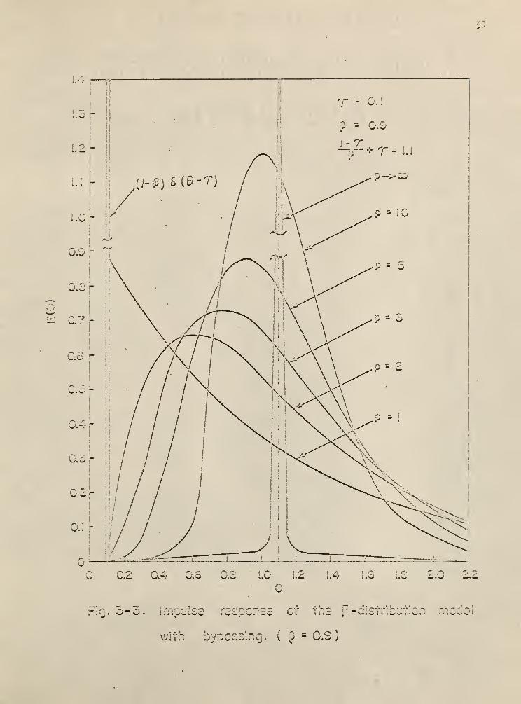
51
,2r
1.0- r
,(j-ej sie-T)
Imnul ^.'»» —
,
I a — ,."' ~..".-»" '-, . ..'.* ~ «,
i I iU\*li\Ji
witr. bypassing. ( 5 = 0.9)

32
tanks in series (p-CSTR). Equation (3-16) is identical to the C curve
for the tanks-in-series model given by (19)
c(e) = >. l\ ):e^1 e^ 6
. (3-17)
Comparing equation (3-16) with equation (3-17) > we can see that
j = p = no. of completely mixed tanks in series.
If
P - 1
equation (3-16) reduces to
Y(6) = e"8
which corresponds to the impulse response of the completely mixed system,
If
3 = 0, t = 1 ,
equation (3-15) reduces to
Y(9) = 6(9 - 1)
which corresponds to the impulse response of the plug flow system.
Step response. A step response means that the input is
X(0) = U(Q ) = unit step function.
The Laplace transform of this input function is
X(s) = |
Hence the Laplace transform of the output signal is
I(.) - X(s)H(s) - {»(&)' ^ & } o— . (3-18)
s 1-t'

33
Lc-
P3K = 0(r—^- ) and A =1 - T
Equation (3-lS) can then be written as
Y(s) {k 1 + L^} e-Ts
Ls(s + A)
P S J(3-19)
Letting
Y,(s) = K 1 + i-ZlJ.1 / . .\P s
s(s +A) P
and writing its inverse Laplace transform as
-1
•CTi<«)
= Yi(G)
the inverse Laplace transform of Y(s) can be expressed as
/-1Y(a) = 1^9 - t)
Y1(S ) can be obtained by means of the Heaviside partial fractions
theorem and the expression can be shown to be (ll)
Y1(6) = K [-^ +
p-1 p-l-v!1 ^ CD
*A* v=0(p-l-^y)i y
^•8^ e"Ae
} (1-3)U(9)
wnere
cp(s)
and
9P-1-Y (-A)
s = -A
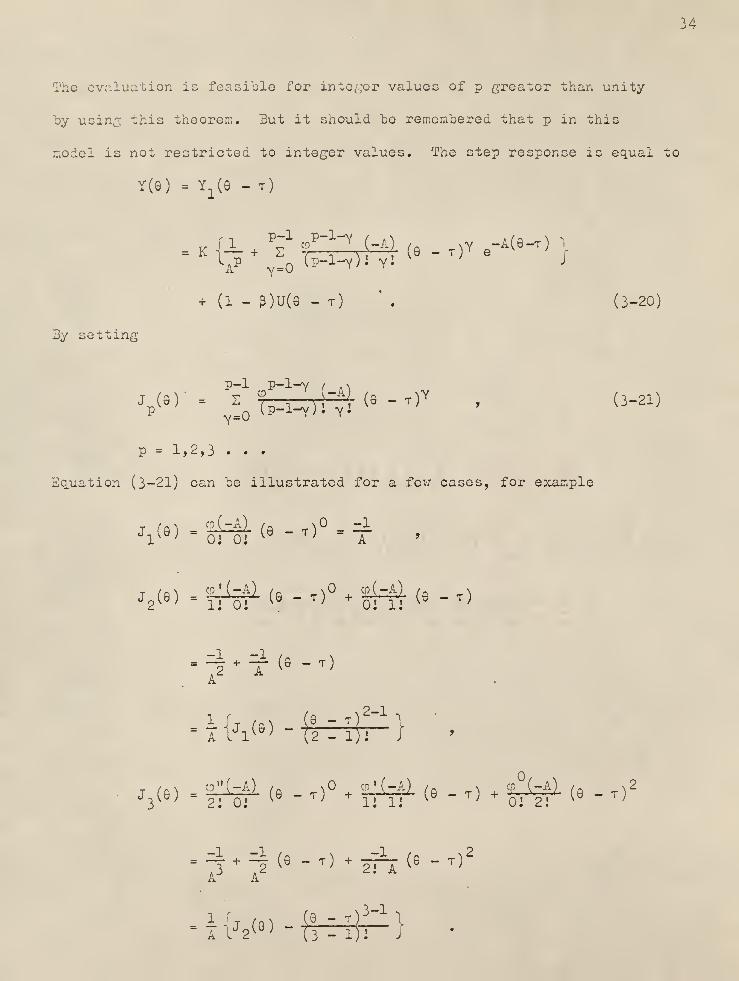
34
3 evaluation is feasible for integer values of p greater than unity
ay using this theorem. But it should be remembered that p in this
model is not restricted to integer values. The step response is equal to
Y(e) = Y1(e - t)
= K |X + ^^(^ (e. T )Y e-A(e-.)-.
LflP „_n (p-I-y)J Y« j
p-1 p-1-y
*A^ v=0
+ (1 - 3)U(9 - t)'
. (3-20)
3y setting
V 9) - %
l
CZ)>~y\ (6 - T)Y'
(3"21)
P = 1,2,3 . . .
Iquation (3-21) can be illustrated for a few cases, for example
j.<e) -*^(e -.t)V ' 0! 0!
V9)' ff^ » ^)° + sHl-
»- t)
AA
iih^-mk-)2-1
^e.)-^#(e- T ) + f^#(e- T ) + fe(e- T )2
AJ A
3 - T)^-1
1
- 1 ! J-HJ2«»-{y^

35
and so on. Wo thus obtain the recurrence relation as
j (e) . 1{j (e) - |» ~ ir1
} •
pv ' A l p-1 (. p - 1 ) J J
Once the value of p is selected, J (9) can be calculated by using this
relation.
Unfortunately, the computational scheme based on this recurrence
relation easily induces an error due to the loss of significant digits
by the digital computer at a low value of . The calculated step
response, Y(G), often fails to show its monotone increasing characteristic
at the initial stage as it should throughout the interval of 9 from a
mathematical viewpoint. The reason is briefly explained below by a
specific example.
For example, at p = 2, the numerical value based on the recurrence
relation is
J2{Q) - ALA " 1J J
which differs slightly from that calculated by the original relation
'2«) " S*'*%^A
The step response is computed by another approach in the present
work. Recalling that the integration of the impulse response is equi-
valent to the step response, we can obtain the step response or the
so-called F-curve by
36
Y(e) = p(e) =fE(e)dG
Hence, integrating equation (3-15) yields the step response
"03
(6-t)
Y(e) = fil&l (e - r)*-1 ." ^ de
o (i-r) pr( P )
+ (1 - P)U(9 - t) (3-22)
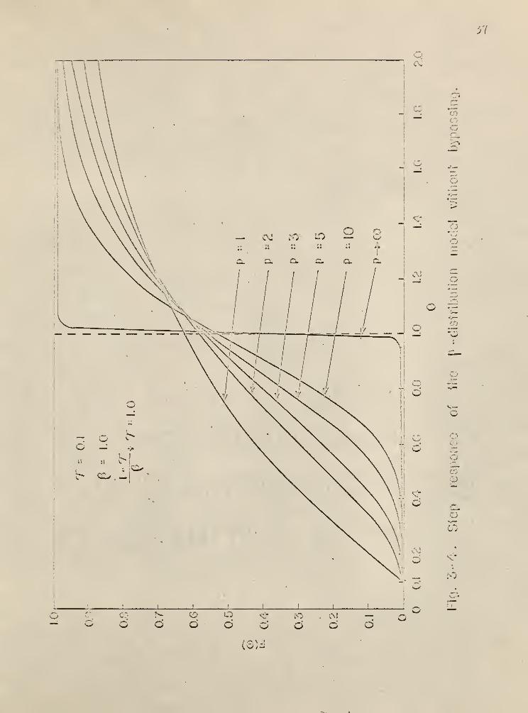
which can be evaluated by a straightforward numerical integration. The
step response curves of two typical s,y stems are shown in Pigs. 3-4
and 3-5*
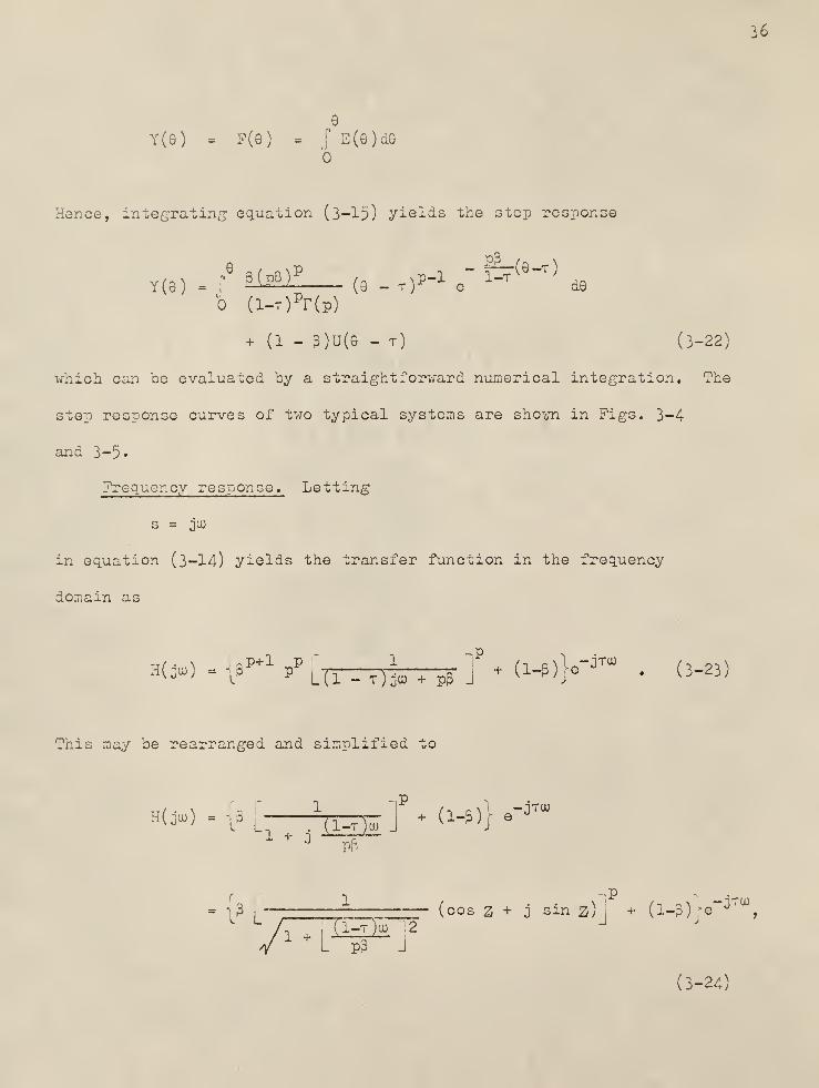
Prequency response. Letting
s = JU3
in equation (3-14) yields the transfer function in the frequency
domain as
H(:.):-L^ 1
p\ (l . T^, pg ]
P.(l-g )}e-^ . (3-23)
This may be rearranged and simplified to
, _ ..p
= "l3 I
' (cos Z + 3 sin z) i+ (1-3) ;e J
,
Y L pp J
(3-24)
57
d d dv."
dc\j
o -
C0)d

}a
"T
J »
__ CO ro if)G
li II 11 11 ;i
-
Q.«
c Q,
o ^_
o o« II
>;^ o
'
-
CO
a
- -
•
v. -•
j
" r
o" lO. — .'.
Is-
6 dv.* TO
dCO
do —

39
where
—1 1—
T
Z = tan (- -a— to)
PP
u) = frequency, rad. /unit dimensionless time.
Applying the Suler formula, i.o.
/ j9\n n in9 n,rt
. r \(ye ) = y e = y (cos n9 + j sin n Sj ,
equation (3-24) is further simplified to
H(*) - « {l (i^tSL f }~ ? o^Z-™>* (l-S)e-J™. (3-25)
Recalling that
e = cos(pZ-tuj) + j sin(pZ-Tao)
and
-1T(J0e = cos too — j sin Ttu ,
equation (3-25) » by expansion and rearranging, is reduced to a standard
form for a complex variable, i.e.
H(jio) = R(co) + jl(u>), (3-26)
where the real part is
2 - £.
R(a>) - {l + 1-^—^- }2
cos(pZ-Tcu) + (1-3) cos tw
and the imaginary part is
2 _ 2.
I(uj) o 3 {l + ^'
~q}
sin(pZ--ruo) - (1-5) sin too
40
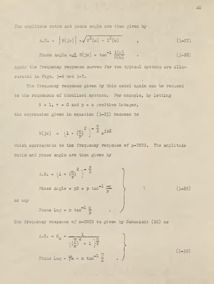
. amplitude ratio and phase angle are then given by
f~2—»
2A.R. = H(jcu) =yR M + I (cu)
Phase Angle =z£. H(jcu) = tan =4—
(3-27)
(3-28)
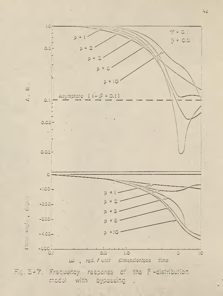
.. ain the frequency response curves for two typical systems are illu-
strated in Figs. 3-6 and 3-7.
The frequency response given by this model again can be reduced
to the responses of idealized systems. For example, by letting
3 = 1, t = and p = a positive integer,
the expression given in equation (3-25) reduces to
2 ,-£TT / • \ -1 fU>\ 2 jpZKu~) = U + (-)
fe^
1. p J
which corresponds to the frequency response of p-CSTR. The amplitude
ratio and phase angle are then given by
i.h..{i + © 2PPhase Angle = pZ = p tan —
or say
Phase Lag = r> tan —P
(3-29)
• J
The frequency response of m-CSTR is given by Nakanishi (22) as
A.R. = G ^m
Phase Lag =
— 2 ,m
jm = m tan —' m .
;
(3-30)

kl
0Ju
5
o
..urrL
0.5-
o.: -r
r
0.05-
-6. F.'cc^^r.cy response of the p - distr: bu:?;cr;
mode! without bypassing .
k2
..^
<
? 5
0.5h Ps 2
0.1
0.05-
0.02-
- <u.\ )
'/
— -ouu
uJ , reel. / unit uirr.cr.c'c
7. Frequency r£zz~.:.zz of
mods! with bvoassino
the P -distribution

43
Comparing equation (3-29) with equation (3-30), it is obvious that
p = i-n = no. of completely mixed tanks in scries
cu = F = frequency.
Thus the expression in oquation (3-29) is identical with that in
equation (3-30).
?.,orients of the impulse response curve for GC1-1';12. Let Y(S) denote
the impulse response of GDMWB in the dimensionless time domain G. The
kth moment of Y(G) is then defined as
m =\ G
1Ci(Q)dQ , k = 1, 2, 3, .
where the subscript Qyk in m . refers to the kth moment of Y(g) indyK
the 8—domain. The Laplace transform of Y(G) is given by
Y(s) = r e"s9Y(G)dQ
which oy successive differentiation with respect to s and taking the
limit as s approaches zero yields (8,23)
dYk(s) '. d:-I
k(s) ,
nxk r" k v / Q \,QIxm —£*—L = lim —r-^
—
L = (-1)__
9 Y(G)a9s -> ds
Ks —> ds"
or
( i \k i dH"~(s) / . . _ >= (-1) lim —r^—<- . (3-3J-;Gyk
s -> ds
This means that the moments of Y(g) can be generated from the derivatives
of H(s) oy taking the limit as s approaches zero. Using the expression
of K(s) given in equation (3-14), it can be shown that

44
lim —-*
—
L = -1s—-^0
o
lim Okl . _ t2
+ 2T + (l-T)2(p+ l)(pp)"
1
s—>0 ds
lin dH(8l m 2t3 _ 3T
2 _ 3T(l_T)2(p+l)(p3)
-l
c—>0 ds^
-.(l-T)3(p+ 2)(p+ l)(p3)-
2
The first three moments of Y(8) are thus given by
.. dK(s)m_ , = u,c = - lim -r—i—<- = 1ayi ^y ^ ds
2
mflv?
= lim £-§LSl = - t2
+ 2t + (l-r)2(p+ l) (pp)"
1
oy2s->0 ds
2
nu ,' - - limd ^ = - 2t
3+ 3t
2+ 3t(1-t)
2( P+1) (pS)"
1
° y3 s->0 ds3
+ (1-t)3
( P+ 2)( P+1)(pP)-2
With these first three moments in hand, we can obtain the (relative)
variance and skewness of the impulse response Y(s ) which is equivalent
to the dimensionless exit age distribution 2(9) as follows:
cr? = f (9 - M- Q )
2Y(9)d9
6y -qp9y'
2
"9y2 ^0y
^ ^ ^ , 2 ds J
s—>0 ds
. -(1-r)2
•»• (1-t)2
( P+ 1)(p3)-1
(3-32)

45
and
a} = f (e - p. )
3 Y(9)d0
= mey3 " 3M,e/ey " »*ey
s->0Lds
3 dsds
2 aS j
= (l-r) 3
L2 - 3(p+l)(p0r
1+ (P+2)( P+ I)(p3)"
2
j . (3-33)
If
p = 1, t = 0, p=a positive integer,
equations (3-32) and (3-33) reduce to
2 p + 1 1o^ = -1 + * = —3y p p
a3 _ 2 _ 3(p + 1? + (p + 2)(p + 1) _ _2_8 ^ P
p2
P2
(3-34)
These are the (relative) variance and skewness of the impulse response
curve (the dimensionless exit age distribution) for p completely stirred
tanks in series. They are identical to the values given for cell
model by Ann (15)
2 1.(3-35)
9y n
„3 2a9y
= ~2n
Comparing equation (3-34) with equation (3-35) > we can again see that
p = n = no. of completely mixed tanks, in series.
Moreover, the (relative) variance given in equation (3-34) is identical
zo the value given for the C curve of j stirred tanks-in-series model
oy Levenspiel and Bischoff (19)
2 IcGy
=j

46
If Y(9) is referred to the pulse response to the input pulse,
) , for GDMWB, the difference between the variances of output and
input curves and the difference between the skewnesses of output and
input curves are defined as
,2 2 2&a„ = cr - a n ,Gyx 9y 8x '
Syx oy 3x
The r.h.s. of equations (3-32) and (3-33) are, indeed, representing
2 , * 3and Lc„>yx oyx
the r.h.s. of equations (3-32) and (3-33) for GDMW33 will be further
t±o r and Lei respectively. More general meanings contained in6yx 9yx u J
clarified in Chapter 4.
Gamma distribution model with overall-cross bypassing. This
represents another modification of the original gamma distribution
model and is depicted in Fig. 3-8. • It differs from the previous one
(Fig. 3-1) only in that the bypass stream is now across the whole system
and joins the outlet stream of the plug flow section. To formulate
the transfer function for this model, the procedure used for the pro-
ceeding model (GDMWB) can be employed. The transfer function for the
F—mixing section is the same as equation (3-11), i.e.
:^r S " Lxr-ffrir]P
•(« 6)
where
-1 V2
3 = -p— and t = —
i transfer function for the plug flow section is

^7
w U -
CJ
! _
-
c o
I
- o
•->-
- o3 O
CO
I..'
-Ha:
CO
ct>
o
<—
o>
O
GJ>s»
-
i•.—
•
• • _.
«5 •. tfl
.—<_ .»-*
^*. oSJ o W~_ 05 <— •.— o•w— o a ~
S3 cy ilj ^-. 3..— Q. • C3 ifi
<.•,> **-
C3 >» ©'"- ».
—
-^
O S3 03 £* &» o<• S O<r^ O
r-•™
*v—
• S)</*
O E JZ. —a :j «a-
C7i -*—
oC/
r— —
>
-;_
o
3
o
-— t J
Ci
"*». *** 1 **li
o
o<£_ «*- —
-
v_;
o o>
>—
'
o Oo
3 3 a ur'i 7~i
*-.—- ou i_
>
I. .

C (s)
P c^R-TS
b)„ = T^rrv = e— . (3-37)
:
2':.c material balance at the point where the bypass stream joins the
outlet stream of the plug flow section is
ofy - ^c2
q2c
Dividing by QT
gives
C3
= 3C2
+ (1 - 3)CQ
I king the Laplace transform of the both sides of the equation yields
C3(s) = 3C
2(s) + (1 - 5)C (s) . (3-38)
3y combining equations (3-36) through (3-38), it can be shown that the
transfer function for the entire system is given by
H < s > ffiy- e
l (i-t) s + P3 J"e_TS + (1 - 3)
'(3"39)
where p, 3> and r are the parameters and have the same physical signi-
ficance described previously. In case there is no bypassing, i.e. when
3=1, equation (3-39) reduces to equation (3-7) > which is the transfer
function of the original T-distribution model.
48

49
CHAPTER 4
METHODS OP RESPONSE
DATA ANALYSIS
Three methods for analyzing response data will be discussed in
this chapter. The major purpose is to fit a model to the experimental
data in-order to determine its parameters. Although the curve fitting
can be accomplished in the time domain, this is not always feasible due
to the practical limitations imposed. In practice, the data are often
transformed into other domains for analysis. Three methods for mathe-
matically analyzing the response data have been briefly introduced in
Chapter 2. The methods will be treated in detail in this chapter.
Each method will be illustrated by an example in which the gamma distri-
bution model with bypassing, described previously, will be used. The
general flow chart of the data processing involved in the three methods
is shown in Pig. 4—1«
Adjustment of the raw normalized data. It is generally recognized
that the response of the pulse testing exhibits a slow decay, especially
in industrial processes. In such cases data reduction becomes time
consuming. Furthermore, the data in the tail part of the response
curve may not be sufficiently reliable due to the error introduced in
detecting and recording low tracer concentration. A general approach
is to truncate the output at a certain finite value (9) and to approxi-
mate the tail from that point on by an exponential decay (12). In this
work (5)5 another method as suggested and tested by Rooze (13) is used.
This is to assume the input, X(o ) , is fairly correct, while the output,

50
Raw data
\(t), Re(t)
Normalize to
X(t), Y(t); X(9), Y(9)
1Adjus-t to
x(t), v*>» x(e), i (e)
j
/ Base d on the criterion A
" -Sx= r0yx
1
Calculate the moments
ana their differences
^ey' ^Gx' 3yx2 2
ay' 9x', 2AaGyx
V aSx'
^o_8yx
v
Calculate the Lapl ace
transform X(s) , Y( s)
and the observed
system transfer
function in s—domain,
i.e. H (s)o v '
__i
Calculate the Fourier
transform X(jou), Y(juj)
and the observed
system transfer
function in w—domain,
i.e. H (ju>)
f
Correlating wi th the
derivatives of model
transfer funct ion
r
Fitting with the
predicted model
transfer function
H (s) <--> H (s)o P
Pitting with the
predicted model
transfer funct
i
on
H (jcu) <- —
>
O >)
i t •i
i Results of the Results of the Results of the
1 moments method of s-plane analysis frequency response
analysis\
analysis
Fig. 4-1. Flow chart of the data processing involved in
the three methods of response data analysis.

51
Y(8), is corrected with an empirical correction formula as follows:
y (e) = py(9)(i - Q9) , (4-1)c
where 9 = dimensionlcss time domain, Y (8) represents the adjustedc
data, and P and Q are the correction factors. If the data are good,
the values of P and Q should be close to one and zero respectively.
P and Q can be computed by noting two properties of pulse testing data,
The first property as shown by equations (2-13) and (2-14) is:
f X(8)d9 =fY(8)d9 = 1 . (4-2)
The second property is that for a closed system the mean of
Y(c), (i,„ , minus the mean of X(8), p,ft
, is equal to unity (normalized
mean residence time), which has been shown by Zwietering (2), i.e.
-By ~ ^8x = ^eyx= 1
'U~ 3)
?rom equations (4-1) and (4-2), we have
fY (8)dG = P
fY(9)d9 - PQ J 8 Y(8)d8 = 1 . (4-4)
o °• b b
5rom equations (4-l) and (4-3) > we have
.!6 y (e)de - f e x(e)de
oc
o
CO
2,= P r 8Y(8)d8 - PQ [ 6 Y(8)d9 - j" 8X(G)d8 = 1 . (4-5)
b

52
If we let
= [ aY(G)d9 ; B =f9X(e)de ; M = [ G
2Y(9)d3 ,
o b b
the solution of equations (4-4) and (4-5) for P and Q, is given
respectively by
„ (1 + B) - I.I r 1 + Br = ' ^ , ^ = - A
2 v ' * " a(i + 3) - :.:
foments method of analysis (8,26). Let Y(w) be the adjusted exit
probability density function in the dimensionless time domain (here the
subscript c is omitted) . Then its kth moment is defined as
m0yk
=«f
Q1CY(8) d9 »
k = 1, 2, . . . (4-6)
and its Laplace transform is given by
00
Y(s) = re"S9
Y ( 6 ) d9 • U-7)
By differentiating equation (4-7) successively with respect to s anc
taking the limit as s approaches zero, it can be shown that
lind" Y
(a
) = (-l)k
m , k = 1, 2, . . . (4-5)s->0 ds
k 9yk
. le mean of Y(9 ) is then equal to
1
9Y(9)d6 = m = - lim gifil, (4-9)
9y.
9yls->0

its variance is
a? = ' (3 - y,a )
2Y(6)dG
oy - ^9y'
^3
= m9y2 ~ ^Oy
lirad2Yl
)
Lds
2 ^-(f^)2
j(4-10)
and its skewness is
CO
?} = r (9 - n„ )
3 Y(3)d9oy
ctoy
2 3
9y3 6y 9y 9y
, _ lia :l^i_3Msi^M, 2(41^- )
3
] .
)
Lds3
as . 2a:
Similarly, it can be shown that the mean of X(9) is
Hid2i
• dX(s)- lim -z
—>
—
L
s—>0
(4-11)
(4-12)
its variance is
dxrd
2x(sl
lira|
—p
s /
s->0 dsMs ; (4-13)
ana its s.-cevness is
3 - - lim,3Y ,2... .> 3
'Qx )Lds 3
xLsl. , dX(s) d X(s) , dX(s) x
^ ds , 2A ds j
J »
ds
(4-14)
54
^reCO
x(s) - \ o"°a
x(e)de . (4-15)
I'.o:: consider the system transfer function, which is given by
H(a) = U4 . (4-I6)
As shown oy Otto (8), successive differentiation of equation (4—16)
yields
Wsi = ^lsl_XV(sl( jH(s) Y(s) X(s) ^ x/;
iWsl _ H'2(s) _ I jHsi _ Y'
2(s) 1 _ ;x^i __
X'2(s) I , ,^ H
2(s)
LYTtTY2(s)
J LxTsTx2(s)
J " ^
H"'(s) _ 3 H"(s)H'(s)x 2
K'3(s)
rl(sJ H
2(s) H3 (s)
r Y:
M(a ) * Y"(s)Y'(s) Y'
3(s) "I
~Lf^ Y
2(s) Y
3(s)
J
.3,
-ff- ^n
'f'B
' t 2^M' . (4-19)LMsjX2(s) X3 (s)
-
Prom the properties of the probability density functions, X(0) and
Y(o), we can show that
lim X(s) = lim J eGa
X(e)d8 = \ X(e)dG = 1 (4-20)s—>0 s—>o b
lim Y(s) = lim j es9
Y(e)d3 = [ Y(e)d9 = 1 . (4-21)s->o c—>o b b

55
Hence
lira H(s) = linn S^f = 1 • (4-22)s->0 s->0 M ° j
3y taking the limit of equations (4-1?) through (4-19) as s approaches
sero and by making use of the relations derived in equations (4-9)
xhrough (4-14) and equations (4-20) through (4-22), it can "be shown tha -
lim f^3
' - -(u- Q - |AQ ) = - A|J,_ = - 1 , (4-23)^„ ds Qy 0x' 9yx '
v '
s—>U
!"'i2^(s) /dH(s) n
22 2 „ 2 /. .,,lim —^—^ -
( ,N '•
) I= cr„ - a c = Aa_ , (4-24;
,- L , 2 Ms ' j 6y 6x 8yx '
s—>0 ds
im r ^H( S ) _ dE(s) d H(s)2
/ dH(s) /^ x* L, 33
els . 2+ ^ds j
Js—>0 as ds
= _( a^ - a\ ) = - AcrJ . (4-25)v 9y 8x' 0yx n "
'These equations, equations (4-23) through (4-25), are the relationships
required in fitting a 2-parameter model to experimental data. Equation
(4-23)? however, is an invariant for a closed flow system and is inde-
pendent of the variation of model parameters and only equations (4-24)
and (4—25) are actually used. The far right hand sides of equations
(4-24) and (4-25) are evaluated from experimental data, while the far
left hand sides are derived from the transfer function of the model
which contains two parameters. In general, n + 1 moments are required
for an n-parameter model.
The moments method described above seems to provide a simple means
of fitting models to the experimental data since this method generally
requires less computational time than other methods. However, a serious

56
fault of this method is that too much weight is placed on the tail
part of Y(6) corresponding to large values ox 9. As has been stated,
. tall of Y(q) may not be reliable due to the difficulties of measuring
tracer concentration accurately at low concentrations. In case it
becomes necessary to use higher moments for fitting a model, this method
tends to become less reliable. Another disadvantage is that the results
of analysis provide no information on how well a particular model fits
the data, unless we choose to compare the response of the model with
the experimental response in the time domain after the parameters have
been computed.
An illustration using G j". .v5
.
The transfer function of the model
as given in equation (3-14) is
By differentiating this equation successively with respect to s and
taking the limits of the derivatives as s approaches zero, it can be
snown that
11- f^" - - 1 , (4-27)s->0
9
limd^ s
)- = - t
2+ 2t + (1-T)
2(p+I)(p3)-
1, (4-28)
s—>0 as
lims—>0 ds^
LJ^l . 2T3 - 3t
2- 3t(1-t)
2( P+ 1)( ?3)-
1
-( P+ 2)( P+ 1)(1-t)3 (p3)"
2. (4-29)
Note that equation (4-27) verifies an invariant of a closed flow system
.•sviously (2). If equations (4-27) through (4-29) are
substituted into equations (4-24) and (4-25), it can be shown that

57
"/_.,w a \-l !
(l-r)-L-l + (pfl)(pP) j = Ac
Gyx (4-30)
(1-t) 3
l2 - 3(p+D(p3)
1+ (p+2)(p+l)(p3)
2
_j= Acr|
yx , (4-31)
2 3where t is the dimensionlcss dead xime and Aa„ and Ao are
0yx Gyx
evaluated from the experimental data.
If the experimentally observed t is used, the model parameters,
p and 3, can he determined by solving simultaneously equations (4-30)
and (4-3l)j which are obviously non-linear. Linearization of the
equations over a limited range by using the Taylor series expansion
and truncating all but the linear terms will be used to solve this
problem. 3y rearranging equations (4-30) and (4-3l) and setting
(4-32)F(p,|3.) = (1-t)2
-1 + (p-i-l)(p3)""1
!
- Act2
= ,
G(p,3) - (1-t) 3
l2 - 3(p+l)(p3)
1
8yx
(p+2)(p+l)(p3)~2
'.
-Act;' =0Gyx (4-33)
the Taylor series expansion around the initial guess p , 5 gives
F(p +Ap,3 +Ap) = F(p ,p ) + Ap ~v± o " o o-' o y ^ Spp ,3* o' o
- o,
po'?o
G(p +Ap,3 +A3) = G(p ,3 ) + Ap ~w o ' o 'VJ^o' o' * dp
P jPo o
+ AB 22. I
+ up -r^r ,
P >Pro' o
where the higher order terms in Ap = p-p and A3 = 3-3 are neglected,
Tag solution for Ap and A3 are then given ""ay
Ap =G(P ,3 ) ~v o' o J
?p P ,3 " P(po'
3o )
o' od3 T) ,3
o 7 o
6P P »Po' o
£Gop
(4-34)
P ,3* o' o
or
o3 P ,3 Qop p~>po o

53
v o' o' Sp--
P^>PO' o
- G(p ,3 )~
v o' o' op 1 o' o
apSG
P ,3 33 P ,P1 o' ocp V 3
o*» o" o
. (4-35)
...se arc used to determine magnitudes for increments to obtain improved
values of the parameters, p and 3. The computing procedure is as
follows (20,21).
1. Guess initial values of parameters as p and 3 .
2. Calculate the increments of p and 3 by using equations (4.-34)
and (4-35).
3. Obtain the new values of the parameters as
i+1p
1 A 1= p + ap
3i+1
= 31
+ A31
4. Repeat 2 and 3 until no further significant improvement is
achieved.
For practical purposes, the correction is initiated by taking Ap and
a3 as one fifth of the step sizes given in equations (4-34) and (4-35)
in order to assure the success of convergence.
The partial differential terms required for computation in equa-
tions (4-34) and (4-35) are given below.
22lS3
- 1 -
^ P
L_ _ -(1 - Tp (p + 1)
apP3
2£_ /i . 7 )3 3p(S - 1) - 4
op' ^ r")
32
p3

59
W /, „.x3 3p3(p »• 1) - 2(p -t- 2)( P + 1)
*F= (1 " T)
33
p2
2 3The values of Aa A and Ac;: can be obtained from the experimental
9yx syx
data as follows:
,2 2 2Aa
0yx= a
9y " a8x
Aa_ = o\ - o% ,9yx 9y 9x '
where
Clj
= m9y2 ' *9y =
ra
9y2 " m9yl
2 2 2
9x 6x2 ox 9x2 9x1 7
9y 9y3 9yl oy 9yl '
3 ,239x 9x3 9x1 9 x 9x1
2it can be seen that the quantities required for evaluation of Ac, and
9yx
Ac;: are essentially the moments of both Y(9) and X(9). In the present9yx a \ / \ / j.
case, the first through the third moment must be found. The moments for
both Y(9) and X(G) are numerically evaluated by'
» - N ,
m. . = '9 Y(8)d9 = S 6 !(6.)A8.9yk £ i=1
i i ; i
wnere
°° k M kn9xk
= J 6K
X(9)d9 = E 9* X(9.)A9.i=l
k -1,2,3
5
?

60
2 1Another method for evaluating ^o~ and Aaf is by
Gyx uyx
ia2
.
9yx
2 2c
4- a.
ty tx" i 2
8yxty tx
i 3
wnere
t = mean residence time,
2 2 3 3 • / \and a, ,c. -, o\ and a, are the variances and skewnesses of Y(^)
ty' tx' ty tx v '
2 3 2and X(t) respectively in the (real) tine domain, a. , c
. , c and
aj can he evaluated by equations (2-17), (2-18), (2-21) and (2-22),
which in turn can he obtained from the few fundamental moments of both
Y(t) and X(t). Recalling that
r Y(t)dt = i ,
we can write the kth moment of Y(t)
ftk Y(t)dt
Y(t)dt
mtyk ^~
Actually, this is true even if Y(t) is not normalized. if values
Y(t) are read at N equidistant points on the time axis, nx . can be
numerically computed as
61
N ks t?y(0i=l
m, , =tyk
S Y(t )
i=l
k = 1, 2, 3
2 3a ± and a, are then obtained byty "cy
2 2 2
ty ty2 tyl ty2 ty »
3 ,23a, = m, ., — 3^, n o*j. - m
a. Tty xy3 tyl ty tyl
2 3 —c x and .ct. are obtained similarly. The mean residence time, t,«x tx
can be measured from the experimental condition as
- Vx =
5
where
V = total fluid volume of the system,
Q, = steady flow rate.
s-plar.e analysis (9,27). This method in essence consists of
fitting the model to the experimental data in the Laplace (s) domain.
The Laplace transform of Y(9), by definition, is
Y(s) =] e"
soY(3)d9 (4-36)
and the Laolace transform of X(Q ) i:
cx>
X(s) = f e"s0
X(G)dG (4-37)6
wnere

62
s = real and positive values.
rical calculation of Y(c), a^ given by Johnson (5), is to
approximate it by a staircase integration, i.e.
.
Y(s) = T, Y(b)n=l
n Y(e) . + Y(e) e
__ T (
r-1 ^n}
rn
e-so ^
n=1 ViN t r -, -s9 -so
n
== 2 ~|Y(e) . + Y(6) (en
- en"X
), 2s L n-1 s 'n J
'
, -s9 n II-l -sS
n=l
-(Y(6)N-1
+ Y(9)N)e"
N} . (4-38)
The numerical calculation of X(s) is carried out similarly. The observed
transfer function of the system is then given by
H (s) -|[f} . (4-35)
the model selected is good enough to describe the system, there
must be a set of parameter values in the (predicted) transfer function
of the model, H (s), such thatP
H (s.) ~ H (s.) , for i » 1, 2, . . . , N •
p 10 1
The criterion for selecting such a set of parameter values is that
the (squared) error function, o, is a minimum, i.e.
N . , - 2
m « S I H (s.) - H (s.) = minimum, (4-40). . L p l o i J ' v ;
re cp is the sum of the squared deviations betv/een the data points

63
"transform equations (4—36) and (4-37) ?where the term e ° acts as
and the corresponding points predicted by the model. The goodness
of fit is expressed by the value of o. Theoretically, it is cost to
fit the data over the entire range of s domain, i.e. 0<_s< co. In
practice, the use of integer values of s ranging from 1 to 10 may lead
to acceptable results. This can be visualized through the Laplace
a
weighting function for both Y(q) and X(o). Generally, the response,
Y(s), has the properties of small amplitude, wide dispersion and slow
decay as compared to the input, X(d). The numerical value of H (s)
becomes smaller as s becomes larger. On the other hand, the transfer
function predicted from the model, H (s), such as given by equation
(4-26), also approaches zero as s becomes larger. This is to say that
a large value of s tends to reduce the effect of- variation of the
parameters of the model. Since fitting the model with too large a
value of s gives no sensible results, it is desirable to select s = 10
as an upper bound to replace s = °°. On the other hand, it is true that
CO CO
J e~s6
Y(8)deJ"
Y(9)d3
lim H (s) = lim - = 1o °° °°
s—>0 s—>0 f -sS v fn \ J3a r» Wo\^e X(u)d8 X(9)d9o b
and
lim H (s) = 15->0 P
This means that small values of s also tend to reduce the effect of
variation of the parameters in the model. This is why s = 1 is selected
as a lower bound of fit instead of starting from s = 0.
By using the same argument, it can be seen from equation (4-36)

64
I
• ;e value of G, the term o '
, acting ao aweightin r^on
for Y(g), becomes very small as 6 becomes large. This is ;.rhv numerically
transforming the Y(g) data into the s-domain tends to reduce the errors
in the tail portion of the response curve (y) • Response curves of the
model can bo compared v.rith experimental curves in the H(s) vs. s plane
and -.he goodness of fit can be expressou in terms of the error function,
z. Tr.aee are the advantages associated with the s-piane analysis. Che
aisa^vanta^e is that the fit obtained does not guarantee the best in
the least squares sense in the time domain.
-. illustration usin,^ C:Xh.3. In this case the predicted transfer
function of the model as given oy equation (3-14) is
V s) 1& L U-t)s
3
+p3 j
?+ (^)}°-7S •
(4-41)
criterion of fitting the model to the experimental data is then
to minimize
- " 12
By using the observed dimensionless dead time t and evaluating H (s.)o 1
from the experimental data by means of equation (4-39)> the two para-
meters, p and 3, can be determined from equation (4-44).
The Taylor series expansion of cp in the neighborhood of first
.. ss, p and p , and truncating all but the linear terms yields* O O sn / \
H (sj = H (s,)| + (Ap)^-P l P l '
fl^'op
P«»P p ?po'' o o o
5H (s.)+ (A3) «JB_i
po»3(
i = 1, 2, . . , K
(4-43)
whoro
A P = P - Pq , £& =* .0 - 3
C>
Let
H (s.)TO l'
^o' o
- H (s.) = Q.o v
i' 1
an (s.)p i
opp »po' o
-, P - (1-t)s.
(l-r)oi
+ p;3;
L ( I-t ) s.^ + p3
-i / PP \1 -ts.1= A.
P ,3
oH (s.)p i
6? V3o
- o1^
(1-t)s. + pg) «±- (1-f )s
±+ p3
"i
- 1 e i f = B.J ^ ,3- o' o
then we have the error function as
co = (Q±
+ A±Ap + B Ap)
The method of least squares states that we should seek an unrestricted
minimum of cp« This requires that
or
r ' r?> Bo
B(Ap) dp= ,
Sep
B3,
Y, (Q. + A. Ap + 3. A3)A. =
i=l(4-44)
::
7 (Q. + A. Ap + 3. A3)B. -- i l 11
i=l(4-45)
Solving simultaneously equations (4-44) and (4-45) gives the magnitudes
of increments for obtaining improved values of p and p as

66
N N IT N2 B.Q. 2 A.B. - 2 A.Q. 2 3
. . i l ... i l . . l l . . l. 1=1 1 = 1 1 = 1 1 = 1 ,. .,s^ ' ;;,:;„ 1
;' u'46 '
1=1 1=1 1=1
-
2 A.Q. 2 A.B. - 2 B.Q. 2 A.,11. ..11 . . 1 i . . lAA i-l i-l i-l i=l („ /7 \A3 = -T3 f— h ' (4-47;
i. _ JN p .. p
2 A 2 B7 - ( 2 A.B.). . l . . l . _ i i
y
1=1 i=l 1=1
The computing logic is the sane as that used previously in the
moments method. An iterative computation is performed until the values
of increments converge to the desired tolerance.
?recuency response analysis (16,17,26). In this method T.-:e try
to fit the model in the frequency (w) domain. The first step is to
calculate the observed transfer function of the system in the uo—domain
from the experimental response data. This is done by applying zhe
Fourier trailsformat ions to both Y(G) and X(o) and taking their ratio
as follows:
r e~^eY(8)dG
rV*06x(e)d9
>H (*») - ^ , (4-43)
or
H (ju)) =
|
Y(9)cosuj3d9 - j [ Y(8)sin u)9dfl
b o'o
KkJ' » »
f (4-49)" X(8)cos U)6d6 - j f
X(6)sin w9d9

67
sre
Let
3 = /=!
cu = frequency, rad./unit dimensionless time,
= dimensionless time.
Y(e)cos w9d8
(4-50)
B =fY(e)sin w8d9
C = ' X(9)cos oo9d9
D = P X(9)sin co0d9
then we can simplify equation (4-49) into a standard form of complex
variable as
H (jco) =A -
ti3
C - 3DAC + 3D . AD - B<
n 2 ^2C + D+
2 2C + D
?he real part of H (jcu) is theno
R (co)o
AC + 3D
,2 ^2C + D
and the imaginary part is
(4-51)
(4-52)
I>) AD - DC
~2 ^ .,2l. + D
The amplitude ratio and phase angle are then given by
A.R. = H (j»)
2 .2 &(
A + B)v o o /2 2
C + D
(4-53)
(4-54)

66
:le =^ Ho<3u>) = tan Vg +
- • (4-55]
can be coon that A, B, C and D are the essential terms needed
for evaluating; equations (4-51) through (4-55) • Since analytical
cessions for X(0) and y(g) are not known, these terms must be evaluated
ly. In order to illustrate the numerical technique which has
. en usod in this investigation, consider the integral A of equation
[4-50) • As suggested by Huos and Donegan (16), Y(g) is approximated
by a staircase type function having equal diraensionless time intervals
and of sue:; height that the area under each step of the staircase
function equals the area under that portion of the Y(8) curve within
the interval. Thus A can he expressed as
n ^e
A = E Y(9) Pn
cos ooGdQ , U-56)n=l
nG nn-1
"..'here Y(G) is the amplitude of the staircase approximation in then
interval between G , and G . Y(q) can be obtained by a parabolicn-1 n n
approximation as (5)
Y(e)n
. i {5?(en_x ) + ar(e
n ) - y(an+1 ) } , (4-57)
or simply ~sj a straight line approximation as
^ 6>n - HY < SVl + Y < S >n }
• (4-58)
mensionless time intervu-, 1G = G - 9 - , is taken small' n n n-1 7
enoug] , t a proximation given by equation (4-58) is satisfactory.
If the e: 'imental data are read with fairly large intervals, approxi-
iion by equation (4-57) is preferred.

Now consider the right hand side of equation (4-56), which, upon
completion of integration, can be further simplified to
69
NA = £ Y(e) t (sin w
n=ln co
G - sin co9 . )n n-1'
CO (JU
N - pE Y(9) - sin ^ (9 - 9 - ) cos £ (9 +9 -
)
- n co 2 ^ n n-1 2 n n-1'n=l
If the dimensionless time interval is fixed at a constant value of
A 9 we havey
9 - 9 . = A9n n-1 y
ana
9 +9 . = (2n - 1)A9n n-1 j
Thus, we finally obtain
y
A = S Y(9) - sin(^ A9 ) cosj
SjL (2n-l) A9,
v 'n co ^2 y' L2 v ' y Jn=l
(4-59)
In a similar manner, we can obtain the expressions for B, C, and D
as follows:
B = n(B) - sin(^ A9 ) sin ' ~ (2n-l) A9 I , (4-60)_, 'n co
v2 y L2 x 7 J
.
'
P
C = 2^(G)m-sin(|A9
x ) cosif (2m-l) ^ j ,
m=l
M~/~n 2 . /Co (•
D = Z X(9) - sin(^ A9 ) sin; ^ (2m-l) A9
, 'm cox 2 x L2 ^ x j
m=l
(4-61)
(4-62)
whore A3 is the equal d'imensionless time interval of the ini^ux data,X vi

70
. the number of steps in the staircase approxii ; the
ta. In general, A3 is not necessarily equal to A0 , ar 1x y
-ore s1 ire required to approximate the output, Y(9), than the
in ut, X(o), i.e., usually
: > ::
Consider now the transfer function of the model, which is expressed
in the frequency domain as
Hp(jw) = E
p((o) + 3 I
p(uj)
, (4-63)
where E (cu) is the real part and I (id) is the imaginary part. If the
model selected is good enough to describe the flow pattern, there must
be a corresponding set of parameters contained in K (joo) such thatP
HpC^) = E ^^i) 'for i - 1, 2, . . . ,J
Again, the criterion of fit is to select a set of parameters such that
the (squared) error function, cp, is a minimum, i.e.
J -
o - £ | Tb (uk) - B (u).)]2
+ l~I (<».) - I ("J.)l2
} (4-64)
= Minimum,
"o^c that J is the total number of frequencies selected for fitting,
.o':z is not related to IT in equation (4-59) °r M in equation (4-6l).
A careful consideration must be given to the range of the value
of tu to be adopted for fitting the model. According to Schnelle (17)»
3 reliability of the real and imaginary part of H (jou) and also t]
amplitude ratio and phase angle decreases as w is increased. 'This can
. ;h the numerical calculation of A, 3, and D.
.• all become very small at high frequency, which in turn gives the
71
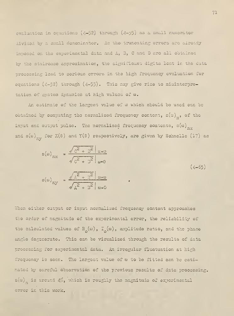
evaluation in equations (4-52) through (4-55) as a small numerator
divided by a small denominator. As the truncating errors arc already
imposed on the experimental data and A, 3, G and D aro all obtained
by the staircase approximation, the significant digits lost in the data
processing lead to serious errors in the high frequency evaluation for
equations (4-52) through (4-55) • This may give rise to misinterpre-
tation of system dynamics at high values of go.
An estimate of the largest value of co which should be used can be
obtained by computing the normalized frequency content, s(cu) , of the
input and out "out pulse. The normalized freemency contents, s(co)
amd s(uq) for X(G) and Y(s) respectively, are given by Schnelle (l?) asny
/ 2 2/ % V C + D I oo=gj
s(w) = —nx
/ 2 2V C + 3 I w=(
(4-65)
(id)sic/TTb* G0=U0
ny /2YA + 3 I uj=0
When either output or input normalized frequency content approaches
trie order of magnitude of the experimental error, the reliability of
the calculated values of R (co) , I (go) , amplitude ratio, and the phase
angle degenerate. This can be visualized through the results of data
processing for experimental data. An irregular fluctuation at high
frequency is seen. ^he largest value of go to be fitted can be esti-
mated by careful observation of the previous results of data processing.
s((u) is around 4$» which is roughly the magnitude of experimental
error in this work.

72
uency response analysis actually fits the model ale
;inary axis, joj, instead of the real positive axis, s,
as ui Ln the --plane analysis. The criterion of fit is the same ac
that used in the s-plane analysis. The advantage of this method ie
as follows, Parseval * s theorem ( 18,28),
Y (t) - Y (t)j2dt = if IyJju>) - Y(j») 2
nb
duo (4-66)
implies that a minimization of response deviations in the frequency
aoir.ain also leads to a minimisation of response deviations in the time
domain. The r.h.s. of equation (4-66) can be rewritten as
^i 2^„ - I r i-,
£ J |
Y ( ja>) -T (jffl)pd» = ±J |x(ju>) H^(jco) - Ho(jco) 'do
This means that the minimisation of the deviations between the predicted
and observed transfer functions in the frequency domain with respect to
a given pulse input gives rise to the minimization of the deviations
of response in the time domain. The disadvantages arise from the fact
that the expression for H (jw) must be obtained by substituting jcu for
s in H (s) and separating it into the real and imaginary parts. This
in itself is a formidable task for a complicated expression representing
the model transfer function. Moreover, the least squares error criterior
requires the consideration of both the real and imaginary parts for each
to, which, of course, leads to more computational time as compare H +.<
he s—plane analysis,
illustration using GDMWB. In this case the predicted transfer

73
function of the model, expressed in the frequency domain, is given by
aquation (3-26) as
H (ju>) = R (ca) + j I (u>),
P &(4-67)
where the real part is
R((jo)=0il +p
v 'I L
and the imaginary part is
(I-t)ucu
Ph
2.-$
j -»
cos(pZ-Tw) + ( 1-3) COS T cu
Lrta
o ii
T / x Q U r (l-r)o; ""H 2IP
(u)) = n1 +L^-pj""
;in(pZ-TO>) - ( 1-3) sin "CJ
cjq = frequency, rad./unit dimensioniess time,
-1 I 1-T v
Z = xan (- —s— w)PP
A iin the criterion of fitting the model to the experimental data is
then to minimize
where
p = Sj
H (jcj.) - H (ja>.) j'
i=I
= £ { ,R (cu.) - R (co.)
|
2+
j
I (u>.) - I (u>.)2
. I L p i ov
iyj L p i o v
i _i=l
= cd(p,3) ,
J(4-68)
IT = number of co values fitted.
As t is the observed dimensioniess dead time and H (,iu.) are obtainedow ±'
from the experimental data by using equation (4-51) » P and 3 are the

74
bwo bers bo be determined from equation (4-66) . Again we should
seek an unrestricted minimum of trie error function, cp. This requires
' ^ = f2. =ap » op
orN -. SR (iu.) ... -, ol (w.) >
,1 L pv 1' o^ i'J 3p L p^ 1' o v i y
j op J
- (4-69)
oR (u).) - -, BI ((D.) ^
E { R(a>.) - H (a>.)| ^ p X+ Fl (co.) - I (u>.) .-?
1r,1 L p
v 1' o v i'J op L p 1 o^ iy
_, op
= . (4-70)II
If the l.h.s, of equation (4-69) is represented by 2 G.(p,{3) and theN i=l
a'
l.h.s. of equation (4-70) is represented oy £ F. (p,S), we have twoi=l
Z
simultaneous equations given as
and
Z G (p,3) = , (4-71)i=l
..
2 P.(p,3) = . (4-72)i=l
thus again face the problem of solving two simultaneous non—linear
algebraic equations. As in the previous two methods, a relaxation
procedure using only the first order xerms of Taylor series expansion
smployed. Expanding equations (4-71) and (4-72) in the Taylor
series around the initial,
[:uess, p and 3 , and truncating all but
the linear terms yields

75
N£ G (p,p)i-1
NE F (p,p)i=l
N &G.
EG,(p ,|3 ) + ApE r-i-1^0' o' , n dpi-1 i-1
N at dF.
E P.(p ,P ) + Ap E r—
^
i-11 ° ° i-1 SP
=
.: 5G.+ A3. 7 , J3
P ,3 -, 00 P ,P1o' O 1-1 '
l o" o
(4-73)
+ A3 S Tq^p )P . , o p "0
, p*o' o 1=1 i -o"o
(4-74)
where
Ap = p - p and AS = 3 - 3
Solving equations (4-73) and (4-74) gives increments Ap and A3
improving initial guesses as follows:
zor
•'
jsr N N SG
Ap =
S G. E ^i-1
Xi-1
op- E P. £
i-1- -1 o,3i=l
I, di\ i^J 6G
i=l**~
i-1^~ - £
i-1
dF,1
NEi-1
op P >31 o' o
(4-75)
N N SG . 1
F. E
A3 =
1 • -, bv1=1 1=1
N oF.
EG. J] tr-i-1 • -, op1=1 1=1
a.1
'
i-1op
JM
>:
i-1
w
OP- £
i-1 i-1op P >3* o 7 o
(4-76)
Again the computing logic is the same as the previous methods.
An iterative computation is performed until no further significant
improvement is achieved. The fitted parameters, p and 3, are then used
zo evaluate the frequency response information predicted from the model
by using equations (3-23) through (3—25). The predicted frequency
responses are compared with those computed from the experimental daea
'o-j using the Bode diagram, which indicates the goodness of fit.

76
>re, the goodness of fit also quantitatively a s 1/. t
value of bhe error function, 9, corresponding to oac;. pair of
tted p; ters, p and £
.
CJovi a Lfficulty arises in that many terms are required in the
. .3. of equations (4-75) and (4-76) for the calculation of Lp and
Aj3 . Deriving the;:; is a tedious task. For convenience in the final
computer programming, additional notations are introduced xo represent
terms which appear frequently as groups. All of them will be derived
in order and given as follows:
Let
1 — TH = :2—r—- o .
P0 '
Y = 1 + H2
,
_ P _ 2X - Y
2= (1 + Ii
2)
2
zr.or. we have
Z = tan1
(-H)
U = cos(pZ - tcu),
V = sin(pZ — too ) ,
we obtain
R = 3XU + (l — p) cos tco,
P
I = 3Xu - (l - p) sin tuoP
partial differentiation of H with respect to p and 5 are
JH -(1 - t)u Hop " 2a " p
p p

77
-(?.. - t)u)
PP
' rentiation of Y with respect to p and 3 are
2?Y -, dHSp oP P
2H --- -—cp op |3
rhe first and second order partial differentiation of Z with respec
•^o p and 3 are
dZ —. aH
ap=
H
OP1 + H
2 Yp
az SH*> -ap
=H
"N _cp1 +
2 Yp
2-s—
'7Yp
ap- H(P-^ + Y)
ap
SP2 "
Y2 2
p
S22
cpc?
_ Y5p
25Y
SYap
>
a2z
YpaHas
- H (3 •
n u
332 "
Y2
3
The partial differentiation of X with respect to p and 3 are
2n. a l v n v— = — - * X InY
2ax t>:-i ;
V " 3Y
partial differentiation of U arid V with respect to p and p* are
._ = _ V (Z + pP)p ap ' '
au. v ^
C-J

76
dp '
T
. ^o:~iJ. order partial differentiation of X, U and. V with respec
to p and 3 are
9 Y / 9TTYdH 2 9Xx „2Y BY BY
2JL ^ a?. 2 _ i(M inY +--
}
ap^ xd op *
.2., Y(H2X + 2pHX fS + pK
2 |S + PH2 P) - p?;
2X fl
- -. dp t-;p dp' -^ E'c
{(2Hxf + H2
f)gT - ^(Y + P f);2 2 2
d? p Y
a2u av/_ szx ../ oz
2z v—= = - t-HZ + p — - V(2 ^r + p —5"
)-^- op op op > d.
o p o p
?2U / dV dZ „ ?Z „ ?-
2Z N—-rr = -(p — rrr- + V^-+ pV ^ >0 ;cpop dp S3 o3 dpdp
S2U /dZ ?V Tr d
2Z x
do o3
>2V dU /„ dZv TT/o 3Z ?
dZ n—^S?^^^ +U(2 ^ +P ~2 }
op
2- -,- -, 2? '/ BU dZ TT dZ TT d Z
dp; . - op - ?.3 * dpo3 '
2 2,dU dZ TT SZ N
S3^ Spdp
2
With all of the above equations ready, ~.'e can now carry out the first
sond order of partial differentiation of H and I with res-oectP P
to p and 3 as follows:
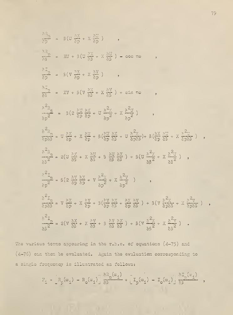
79
• - 5 { J r— -l- X v— ) ,
ep cp op
— = XU + 3(u|f + x|2) . costcbP O fJ
3(v^ + xH)-TO
dp " N' dp " b~o
dlp ,rTr _ /„ dX v dV \r^— = XV+P(V^r-+X^r-) + sin tgj ,
op O P OP
2
P _/_ r-U ijA TT O -- v O U \
7T- = 3(2Ii:s7
+ J— +/-— ;
op ap Bp
-V '-TD O OT> tt OA „ o/OU OX -, A. \ /OA dU v J \
opop Sp dp dp d|3 Bpcp ^Bp d$ cpop
2.
JP / TT dX Y oila dU dX x /
TTr2X T o
2U v—5*- = 2^U ~ + X —- + P ^T ~ ) + 3(u —p + X —5-
; ,.„<: dp op op op ^ n ^ ^ Q ^dp op op
a I 2 2• d w, ov ex „ ax v a v n——- = p ( 2 — — + V —5 + X —-5-
,-^ °? op a d ^ ddp op dp
2.5 -^ „ ax v dV Q /dV ax :
:: dV N Q/Tr a2x
cpop op op op dp op op opoP opop
.2v
- 2-r
j3 / Tr SX _ BV Q dV dX v D ,.r
d2X _ c
2V v
5— = 2(V —-+XT-^-+p^-r-^r) +p(V 5- + a 5- )
-^2 cp op dp op ^ Q 2 -so 2op cpop
The various terr.s appearing in the r.h.s. of equations (4-75) and
(4-76) can then be evaluated. Again the evaluation corresponding to
-. dR (u>.) -
'
., ol (00.)
P. = R (u>.) - R («.)I
.~P 2
+i
I (».) - I (cd.), ^ 1
1 L pv
oh o v id S? L p 1 O v ij op
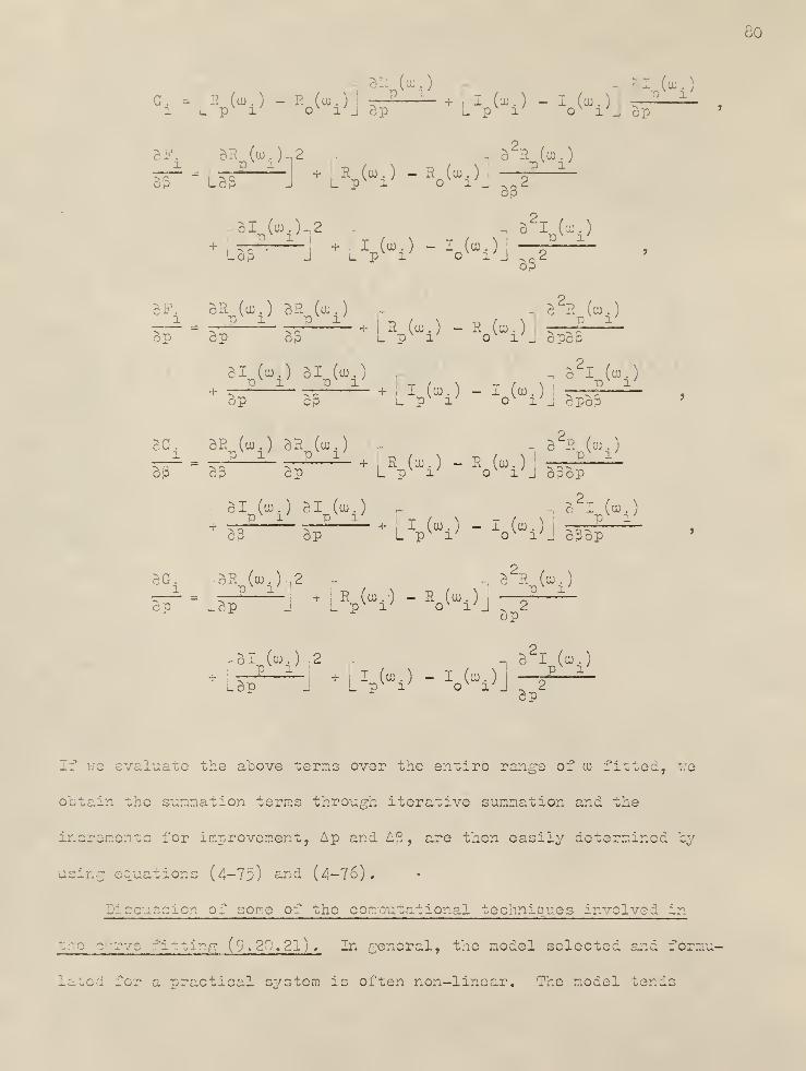
60
-, oR (cu.) • n hi (cu.)
G. -jH (cu.) - R (cu.) + , I (cu.) - I (cu.) ——i-
c. ,-,2 .. B^R (u).)^ = ^P ~ ' + R (cu
.) - R (cu . ) . jr2 —
op LB3 j l_ ^ov
iJ o
vi y
J _ Q 2op
si fa )_2 a2*„K)
Lo5 ' J L p i o i J -, c 2op
BF. BR (cu.) BR (cu.) - _ B2R (cu.)
+ R (id.) - R«(uj.) -Bp Bp op i_ p i o v i'J cpB&
BI (cu.) BI (cu.) .- B2I (cu.)
+ t TTr + r>J - i (u)jap c0 l p i cr i'_ apap
3G. BR (cu.) BR (cu.) - B2R (cu.)
•^— = — T—
"
+ R (.OU - J - R (lU . ) r^rr;o? op op L p i o
vl j BoBp
BI (cu.) BI (cu.) - - B2I (cu.)PI P 1 It I \ r / \1 P 1
cp Bp L p i o v i'J B3Bp
^G BR (cu ) ,2 - ^-\>Jr-i - ,
? Xj
+j
R (cu.-) - R (cu.) ,?
x
Bp lBp J |_ "ov i' o^ i/J _ 2
op
-BI (cu.)-,2 - B2I (cu.)
+ ap X
1 + ,I (cu.) - I (cu.) i
P x
LBp J L p 1 o v i'J - 2Bp
>
- evaluate the above terms over the entire range of cu fitted, we
obtain the summation terms through iterative summation and the
increments for improvement, Ap and £3, are then easily determined by
using equations (4-75) and (4-76).
)iscusr;icn of some of the cor.voutational techniques involve:! in
- -i -'i.-.'/. :• (9 . 20. 21) . In general, the model selected and form;
2 . for a practical system is often non-linear. The model tends

61
to increase its complexity with the increase of the number of ster
con* d in it. ,.c thus face the problem of non—linear regression.
Consider now a general case, that of a model containing n parameters.
Using the moments method gives rise to n simultaneous non-1 3ar
tl ebraic equations to be solved. Linearization of the equations by
using the Taylor series expansion and truncating all but the linear
terms yields, in general, the following matrix representation:
J3Ac/ = _b_
,
where
Z = an n x n matrix
Ac = an n x 1 matrix, step sizes of improvement for n
parameters
b = an n x 1 matrix.
Phe step sizes of improvement for n parameters are then given by
^ = £} ±~ » (4-77)
• Hw — ~~>
Z = the inverse matrix of __Z_ .
'lie improved values of the parameters are thus given by the recurrence
relation of the following form.
ia1" 1
= JL+ %L > (4-73)
.re
_cx_ = vector of parameter values at the ith step,
Aa = step sizes vector for correction at the ith step,
i+1 • j - n ., / . , \ .,c^ = improved vector oi parameter values at tae ^l+ljth
step.

62
Lon procedure is as follows:
1. n initial vector of parameter values as a*.
— ] i i2. Calculate (Z ) , b and then obtain La by using equation
(4-77).
3. .. the improved vector of parameter values, a , by
using equation (4-78)
•
4. >eat 2 and 3 until no further significant improvement is
achieved.
In using the s-plane or frequency response analysis, a criterion
for evaluating the values of node! parameter is to minimize an error
function, cp, i.e.
cp = o(c0 = minimum,
..re
a = vector of parameter values.
The necessary conditions for an unrestricted minimum require that
T77~ - , j = 1, 2, . . . , n
:
This again is a problem of solving n simultaneous non—linear equations.
In a similar manner, the previous relaxation procedure may be applied.
use of the Taylor series expansion for linearisation yields extremely
- convergence' once' it converges. Nevertheless, this method has its
prac - Imitations when the number of parameters contained in the
somes larger. The evaluation of the inverse matrix of _Z_ becomes
.,' cumbersome. The so-called gradient technique may also be used (30)
.
- terative algorithm for this technique can be written as
i-rl i . i- _ ia = a + k V;p

83
wnere
ct - vector of parameter values at the ith step in the search,
k - step sise factor at the ith stop, a negative value for
searching the minimum,
Vo = gradient vector of the error function at the ith ~tep
in the search.
'The number of iterations required for converging towards the minimum
is, in general, more than the preceding method.
In case the calculation of derivatives involved in the above methods
becomes very tedious, the direct search techniques currently developed
may be applied. However, it is expected that a much greater number of
iterations are required than the two methods described above.
The curve fitting procedure is, in general, carried out by the
digital computer. The analog computer' may help with part of the data
processing from an on-line viewpoint (4) but has its practical limita-
tions in the final curve fitting. In case the parameters contained
in the model are more than two, a direct search on the analog computer
by adjusting the potentiometer setting is a formidable task. It is
especially true in this work in which the fitting is not restricted to
boundary point fitting. Moreover, difficulties arise in scaling and
programming when the model is highly non-linear.

o4
5
A [OK PC LIQUID MIX
ON DIST3XLA I lYS
sri mtal work was carried out by Johnson Tor studyin
characteristics of liquid nixing on distillation trays (5)» I- his
investigation, the air-water system and sieve plates with circular
down-pipes were employed. Radioactive phosphorus, P , was used as
the tracer. The investigation included the effect of five variables.
. sy -..'ere the liquid flow rate (L) , the air velocity (V), the weir
height (H) , the number of holes (N) , and the hole diameter (D). face
variable was allowed to take or. two different values, i.e. level 1
(lower value) and level 2 (higher value) . Data were then taken for
eacn possible combination of the five variables at both levels (values,
,
; is, for 32 different combinations. Two replicate runs (2.) were
made for each combination, giving a total of 64 experimental runs.
The (LV] - )notations used to indicate the experimental conditions
are explained in fable 5-1 • For example, the experimental condition
denoted by 112111 means
liquid flow rate (L) 3.29 gpm.
air velocity (V) 21. 7o ft. /sec.
:.oir height (H) 2.25 inches
number of holes (K) one
hole diameter (d) 3/lo inches
re >licate (R) first
a distribution model with bypassin.(
iV3) described in
iter 3 was selected to fit the experimental data according to tee

5-1. ] : of the experimental condition,
B5
Level Level
flow rate (L)
air vticciiy (V)
b ( H )
cor of holes (l\)
hole diameter (d)
replicate (R)
3.29 gpm.
21.76 ft ./sec.
1.51 inches
1
3/l6 inches
first
8 o C0 gpm.
2.2^ inches
S
l/L inches
second

66
i son (5)« In this work, two other . 3ds of
>nse da to his c:-: jntal data oy using
ame model . The results of fitting the model by u
moments method of rsis arc presente _e 5-2. The requite of
Fit the model by using the s-planc analysis by Johnson (5) are
reproduced in Table 5-3« The results of fitting the model by using
the frequency response analysis are presented in Table 5-4.
In order to illustrate tnc goodness of curve fitting ~sj using the
frequency response analysis, the data and results of analysis for run
31 are plotted in the form of a Bode diagram as shovm in Fig. 5--
•
Since each method of analysis was based on the same 64 runs of
rimental data, the characteristics of the analysis can be visua-
lize! through the distributions of the fitted parameters, p and 5,
resulting from the use of each method. For the purposes of comparing
the distribution of the fitted parameters by the three methods of
oresponse lata analysis, the mean ((J.), variance (o ) and standard
deviation (a) of the fitted model parameters from each method are
calculated as follows (29):
_: ::
n. s p.1=1 1=1
i
^ " N "p ":. >
:; n
S (B, - nJ2
2 (P, - l*J2
1 P 2 i=lx ?
__ a _o
ag - V C
3 '
CT
P
-. - .eta! number of aata sampled.
' - 3d in Table 9-5.
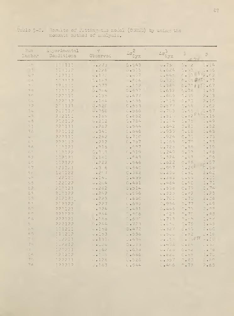
of i >&el (G
momen bs n .or' aj ial;y si: .
L
Conditions Observed~cr.
0yxAc
6yx P p
• • 1 • J. H
. . . 6
0.0.' f . 38 #* . "
•
. 70/ ! . 6 7
c .6
'
.
.40 2.
2.;. .577 2.
—, , ,
1.51.55 1.5.82° 1.1
: .
:
0. ] .49J .642 3.32 1.52D . 9 3 5 1.4 3
0.92 4 0.71 1.721 . 1 0.7 1.3 3
j. 728 '. 1 .
. : .'-
. ?2A n.
C .622 0.
1 .29^jL . 5 7
C . 9 . . ^ w
• 2 5 a . 30 2.420.383 0.94 2.01.. .48 4 0. 1.71- . 3 3 c c. 1.74C . i 0.82 1.2 5
0.76 . 2 .
3.77 ] .491 ."
. 5 2 3 V
C . 7 ] 3 0. 1.58.
: .
. .
.
• 4 . ....
- |.
0.826 . 5 5 . :
. .-
- .
' ,4i ? . 6 5
I Q
-3
4 5
5 7
i
6 2
6 3
-
c; '-
-/ a
1 .1 ]
]
11211]
- -
j
i 2 ?
211111: 12
2121' .
212112221111; .
22211 :
? ? 2"
11112]177
1121 2
]
11212 2
1 2 ] 17. ]
12 : 1221221211221273 1
"
2111221 21
v -
2 1 2 7
7? 1
117 7
7 7 7] 7
]
• 1 2 7
211
1 7 1212i 22;
3 2 2 217
. . i
V.
-
. 3 7 7
.' . 3 4
( -
; .
-
U .
u -
• > .212. 7 8 2
j .34 1
. 7. 4 ?
.71 7'
.3163 .'
. ] r ".
.722/
.2' 7
^ . 141•^ . 2 04w .2 82.. .232, ., .
.7717
.324
. 3 '• 4
. " ' ~
.244-
\J . 153.
.
.
j .
.
.16:
. . " :
:
-
.
.. .
. . '
. 4 7 /
'» .
r.
.366: .852-
o .7 64.
!
: ..
i
w .7 13'
.757
-
„ .543.
_ . 5 4
c .3c2J • 439.481
L .514V .596.60
( .693r~
.
.5 06'
.
'
3 .
..
[
3' -
-
. 6 3 8
.
.
3 . v 4 4

-. .
o6
;al
Conditio-
.
T
9yx yx p
. . . ' . '1 .70
. • c .
. . .
. .'
. " •
• .'. . . •
7 2 1 2 : ? . . . •
- . . .
-22, . . --7 r/ 1.411 1 . - - c . .
- 11122 2 . . . •
-
22] . c. .
- 12 22 2 . ] - • . 0.- - • -) n # 6 2 c 0.
'
?.26- ' - ~
: („••
.
p -> . .
. " 0.'.''
->p 2 7 . 1 : .5 47
. 2 7. \.- :
.'
17. . ; . . : .
} .:
? -
'
; ?
:
.121 . . .9 '
. ] . . . -'- • -•
2 212 2 2 - . 2- .-
:
i.<
2'
.'
i:• . 4 i 7
? 2 ? 2 ? 2 . 1 51 : .^b° ?. ? . 8 7

Table 5-3. Results of fitl models-plane analysis.
by ;ne
Run mtal T3 P
• .-or
106Nu ber Conditions Observed id .'.
7 :l i I 1 l 1 . ? ] . ? r
1 1 "! "5. 2, . .
' --
1 1 ?1 ]
1
." 1.29 .
n?: ] . • : .. '
.
i ] .3 c. 2.12111? . i . :.. -
. ] ] . 4 :
. 1.2] 3.3;'; p .3; 2 . 1 2 5 2 . ( r
- - i 7 .
-
2 . ?~v 13.4 ?
"3
? T ? 1 1 ] • C.89 • • n.74-) - 7 1 1 ?
.
,o? PCo 1.0°
7 7 ] 1 1 '
. ?3? O £• 1 ,'2 ? . 2
-'
-. ^ ? 2 1 1 1 ?" .341 - 1 .74 :
" ..
"'C . 7 7 1 . ? 7
] ? : .2 .66'.
.. . I
•
.25'
1.02 : .• " .429 1 .is: C . i . 1 1 2.
•,
];;
7 .222 :
.
1.46-
* _
^ -7
; ? ] .•- •'-
]
.
. 8 4 '.'-'- S
} 17? :• ?' 7 ( .c 5 ".
. ? 8 2 ." '-'
121 C.< : .74 6.~-1 7 ? i 7 ? ).2 - 0.287 1117] . 7 p 7 r, on 1.2-0 0.4]
112 2 .2 92 1 .- 3.71' ~
1
1 .2 0. 1.2 1 : .
2 21.121 .324 .<
'
] ? / . 3 4 4 ( .72 1.8 4 4.0?? 2 2 1 2 1 C .96 :
.
.
? ? ?1 2 2 . * ]
.
0.34£ r T
-J -J 7 t -j . 1 * 6 1 CO•
111'?!?' "? .(
7 ?1 1 7 ? 1 1 .
''
- .r
1 1 . q 9 •
• 171? .17 6 '
. 9 6 • 7 . 2 n*
' t - - -
2 i ] .162 . 9 1 .. :
.
' '- 1 ? i ? : ? 1.161 ? ? 2 1 ] . 3
- 0.9 1.7? . 64' ' /
] '.16:. . ' i. 2.14
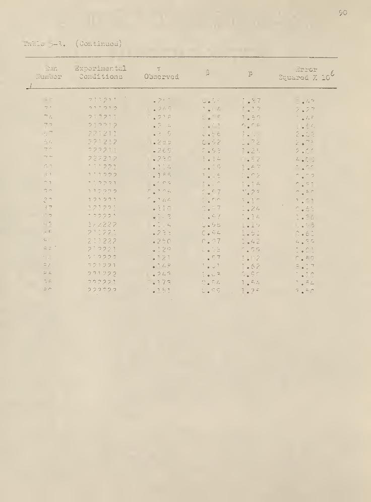
i
r
U.
fcal
Conditio Observed•or-
.10"
. u • .
?n;.
•
• -
. - 9 -, -
•
; •r
i -
, . . .
L 2 1
2
. ). .7!-
]".
..
. . .
tit; )• •
i
-
] ?2? .
--->--.!. r
.
2 2 . r.zi- - - -, - ,
-- • .
-
0. ', 2 A .------
. ] .
"
- § I J H i • 1
9
.
;• 7-
J. 5 C.94:.2 . :
.
4.2
"
? 2 2 1 . ] .
' " ? 2 2 2 .97 C#5 q
? ? i 1. -
"
122 2 • '••'"•'
. 9'
] .K2 2 2 2 2] .17^ '
! .n A • —
•)?)??')w • V 1 .
1- ^ ^

5-4. model (G . theency response analysis.
Sun erimentalConditions Observed
-•or
Squared X 10
3 2
:
-
7 D
7 .-
"' -
inn .1
. ;. 5 0.' 3.14
. 1
'
] . ] . '- 7
1 l 2 1 t 2 ] . ( 1 . 2 3
C . .
] 2 ".
! . c. L.3 .
1 2 2 I
.
':
. .!1 2 2 1
.
• .' -'
•
] j . 3 7 C . 9 2 1.06 2 . 3 6] p
".- 4.71? ? ? 1 -1 1 • ^.7 9
7 12112 •
. ? 1 7 7 . P P^i"i .2ft 2 ^ 9 r , 4?? p 1 1 1 2 .34] 0.79 • 1
722 .242 :;.64 1.' 2.63222: ' .212 C.95 6.J. 1112] 0. (
.",•:' 2 .
"-72 . 3 C 3 2.26 C . : 6
1 12: : C .
'
l.C .;-
-
1.12122 .722 0.'
121] r
;.3::6 1 . c 1 • ... -^ . 7 8
12112 2 .2 C . 9 7 1.11 1 .531 7?i 71 r .141 i . .
1
1 .67 1 .07- -, -,
i •> 9 • .2 04 1.00 ] .27 0.71117] ; . 2 R 2 1 . 1.0! ~.? n 1 ; ? n .792 .Q] 1
.-. 7 "
71712] .223 : . a 6 C .7
'
212122 .227 0. 0.12] . 3 2 4 0.
-
. . - -
2 2112 2 . 3 4 4 c . 1 . -
7 2 2 ] ..." - S 1 .1 0.222] 72 . ".' ."
.
11] 1 ] . 9 6 1 . 4 6
111717 "
. 1c ? 1 ,< r
• *i -
c
117 211 :' .1^1* 3.2~
1 1 ? 7 1 7 ' .12 6 ! .Q9 1.28 2 .
D . 1 6 2 C • 9 6 . 161212J 0.1 • 1.C0 - .
' 1n
: . ? f- 1.2?17 7 212 . . i '- -3 1
. ] .c 1 1.76
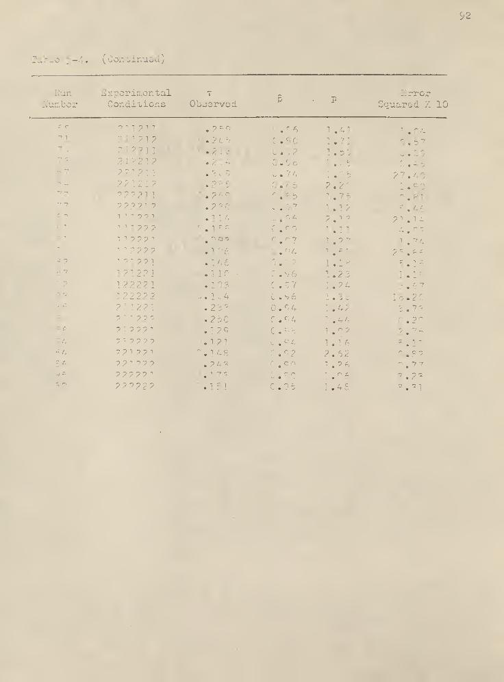
92
- .
un sntal Tp P
ror... Condi aor.c . Squared X 10
- i 1 -;. 1 -
• 1 J
•
. -1
3.
:.
.
.', o -
.
c
.
2., ".
-
9 p " p 1 1 '
. 'f DC
• : . '
"' "7;
i-
•
. 2 3Ci 2 p ] . ] 1 /« -. ?.!
:
?i .:-
-i i p p p . i .] ] 4.09
i i p p
;
C.9 71
1 7 72. ?-
.
-
? P j .146 • *
1 2 . "...
"
i 0.97 1.242222 - . ] C «. 9 6 .!. a ^ _ .
::.2 .r - : . < ; . 7
-] . 2 ! r
.
c k" -
]
~2 7. 1 0.12 9 C.
'
2.7^? 1 p p ? p . i /
ni .
c - -
• I
. ? p 1 p p 1 - 2. r,m g ?
'
? p i p p p '
. 1.2 6• 979791
:• . 1 ? 3 . . 1.9 6 ".z-h n pppp . ]
r q c] .• .3]

i.O
0.5
0.1:
L * I~.;. j::;J. values
GDMWB
T * % 2 8 Z
0.874
cj
ou , rcc. /sec
Fig. 5-1. Curve fitting to the experimental dc4*a from
Run 31 by me frequency response andysis.
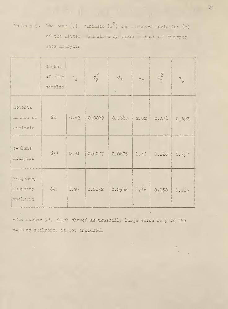
-5- The ...: rice (a", •. devj ion (cr)
ir< 's by three lods of res
. is
ber
or data
sampled
or. a3
f"
.-"-
ts
method of 6:;
i— >—— ,, ~—
—
0.82 0.0079 0.06 2.02i0.478 3.692
s—pi
analysis63* 0.91 O.C077 1.0875 1.40 0.128 C.357
j'rscuc
ponse
anal; r ci_
64 0.97 0.0032 0.0566 1.16 0.050 0.225
Lumber 32, which showed cr. unusually large value of p
- - ne analysis, is not included.

95
1, Using the moments method of analysis, all cases except run 57
e values of p greater than unity and values of 3 lose than unity.
. 37 gives (see fable 5-2)
t = 0.30o , Act? = 0.540 , AoJ = 0.997oyx t/yx
and the fitted parameters
3 = 1.29 > 1 , p - O.58 < 1
: unusually large value of Acu, (high skewness to right) with respectyyx
2zo giver, t (fraction of plug flow) and Acr _ (degree of spread or disper-
sion) means a very clow decay in the response curve. This is why the
computed parameters show a value of 3 greater than unity (correspondin
to the effect of recycle) and a value of p less than unity (the order
of the transfer function is less than one which is the limit case of
completely mixed system). In general, curve fitting by the moments
h - - yes rise to results indicating a higher degree of bypassing
a lesser degree of mixing. In other words, this method leads to
;her values of (l—3) and p as compared to the values given ~oy two
other methods of analysis. The mean values of (1—3) and p for the
moments method of analysis are given in Table 5-5 as
|i, D= 1 — \i a
= 1 — 0.32 = 0.18 = 18$l—p p
|jb - 2.02P
3 can be interpreted as the introduction of truncating error, which
ns the res lonse curves were read prematurely. In other words, we
.ected the effect of clow decay (the tail part). We thus-.23--'- ••' --- ^a
Qyxand
- ^aevx'
v-"- c - : in Tarn leads to the higher values

of (l—p) an 3d to obtain : s-plane aj
or tho frequency res Le 5-5)
•
s (5)> values of p greater ti
..uoo oT P less than uni;;y are obtained in almost all cas
.. a few runs (fable 5-3) • Inte er values of s r from I to
tted. The least squares errors are aro ., >rder )f 1C .
is omitted in computation for constructing Table 5- 'es
- 5-3)
, p = 20.36
le the corresponding replicate run 34 (under the sa^.e condition
of operation) gives
- 3.62 , p = 2.23
The unusually nigh ^evia^ion of the p value in run 32 fro 3 p value
. be attributed partly to random experimental error -..
partly to the inherent error in the data processing procedure (5)« --'-
curve fitting by the s—plane analysis gives rise xo results
Le --ree oz mixii
. ou -.o the values given by the moments method of analysis. The
mean values of (l—3) and p for the s—plane analysis are given in
laoxe p—
5
rn = 1 - ut = 1 - 0.91 = 0.09 = 9% ,
|i = 1.40P
3. Using the frequency response analysis, values of p greater
than unity and values of 3 less than unity are also obtained in almost
-.11 cases except a few run. 1 5-4) • The range of the frequency

97
Lepends on the jxperimental error in oacn run,
Lch car. be visi i through the calculation of S(u)) ( coo 3r
4). In this work, a maximum of 22 points, ran - from cu = 0.01 rad./
sec. to u> = 10 rad. /sec, were fitted and. a minimum of 17 points,
r . -- - from j = 0.01 rad.. /sec. "00 uj = 5 rad./sec. , were fitted.
The range of frequency fitted differed from run to run, re from
17 points to 22 points. The least squares errors given in Table 5—4
are around the order of 10 , "which is higher than that of the s-plane
analysis. This does not r.san that the accuracy of curve fitting
the frequency response analysis is poorer than that of the s—plane
analysis. Ol-.o comparison can become meaningful only if we return to
time domain. In general, results of the curve fitting by the fre-
quency response analysis shows the least bypassing (1—3) but the highes*
ree of nixing as compared xo those ~oy the other two methods.
mean values of (i-3) and p for the frequency response analysis are give:
in Table 5-5 as
\xlmJp
= 1 - |A . = 1 - 0.97 = 0.03 = 3$ ,
|i = 1.16P
Comoarison
.
21. The mean (u), variance (o"") and standard deviation (o) o:
he fi ar .. 3ters given by each method as shown in Table 5-5
eveals th .
) - C.62 < GO = 0.91 < GO- = 0.97m p s pi
(a|V = 0.0079 > (or?)a = 0.0077 > (a?).. = 0.0032
p Hi p •-> pa.
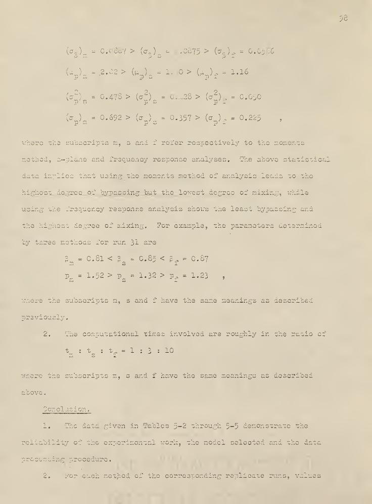
- O.C887 > (aQ ) - .0875 > (Ox. = O.0566j s
...- -' -
> fcp>s " x c > kp)f = 1 ' 16
(c^) = 0.478 > (c-;)f
= !8 > (a^) , - 0.050p s pi
(a ) = 0.692 > (cr ) = 0.357 > (a ) = 3.p ... p o p -
. cripts m, s and f refer respectively to its
method, . - frequency response analyses. The above statistica
the ne_] bs method of analysis leads to. the
ire_e of bypassing but the lowest acuros of mixin . w -le
using the frequency responds analysis shows the least bypuscin;; and
the i Dst degree of mixing. ?cr example, the parameters determined
by three methods for run 31 are
i = c.61 < 3 = c.85 < a . = 0.87r.. s t
p = 1.52 > p * 1.32 > p„ = 1.23 ,m s 1
3 subscripts m, s ana f nave the sane meanin ;s as clescrifc
previously.
2. The computational times involved are roughly in the ratio of
t : t : t „ = 1 : 3 : 10s i
where the subscripts m, s and f have the same meanings as described
above.
1. 2 iata given in Tables 5-2 through $-5 demonstrate the
of the experimental work, the model selected - id ;he data
z.
2. For . jthod of the ccrr: re licate nuns, values
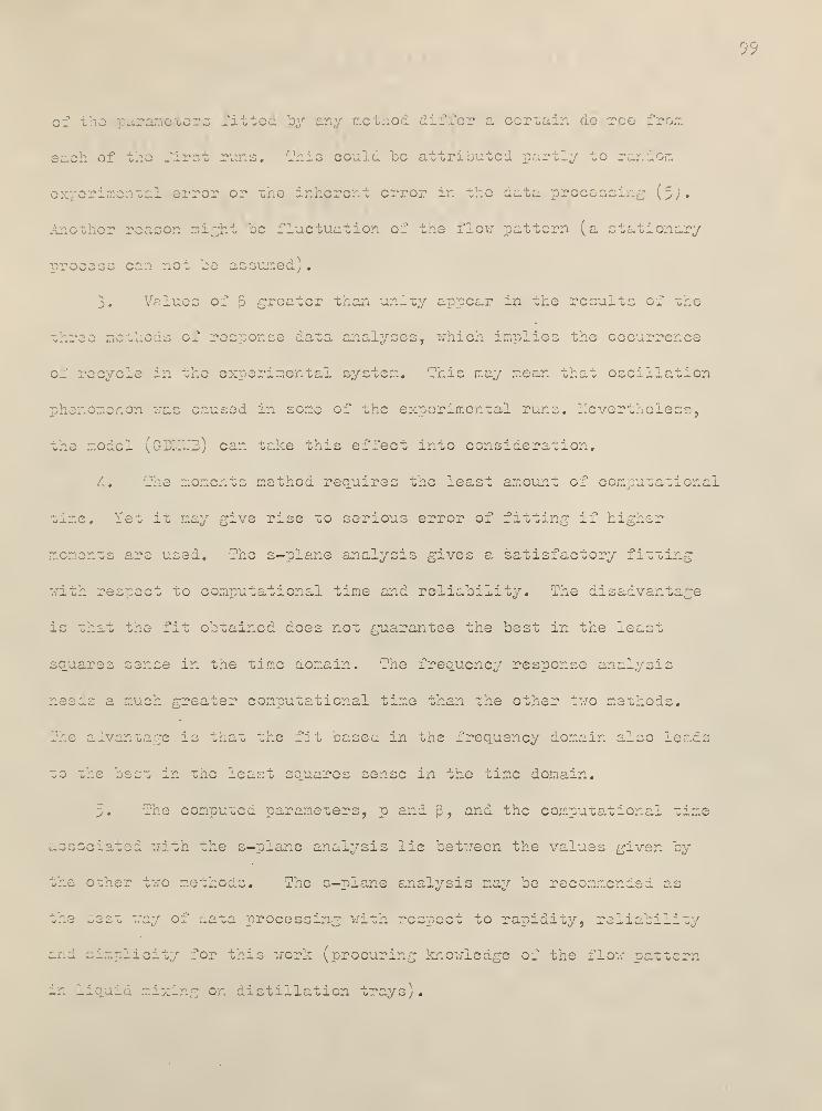
.'or a cer ••>::.
of tho 'ir it runs. This could be attributed ] ri: ;o :: ... 10m
_ error or the inherent error in the data proce ; (5).
Another reason might be fluctuation ow pattern (a stationary
process c; ot be assumed).
3. '.' lues of |3 greater than unity appear in the results of
three methods of response data analyses, which implies the occurrence
of recycle in the experimental system. This nay mean that oscillation
phenomenon "as caused in some of the experimental rune. Nevertheless,
can take this effect into consideration.
The moments method requires the least amount of computational
time. Yes it may give rice to serious error of fitting if higher
moments are used. The s—plane analysis gives a satisfactory fittin ;
with respect to computational time and reliability. The disadvantage
is -fax tho fit obtained does not guarantee the best in the least
squares sense in the time aomain. The frequency response analysis
needs a much greater computational time than the other two methods.
;e is that the fit based in the frequency domain also leads
to the best in the least squares sense in the time domain.
5. He computed parameters, p and 5, and the computational time
associated with the s—plane analysis lie between the values given 'c-j
the other two methods. The s—plane analysis may be recommended as
the ^zzz ray of aata processing "ish respect to rapidity, reliability
and for this ~..rork (procuring knowledge of the flow
mixi . tillation trays).
u a - v _._'.
.

100
ACKNOWLEDGMENTS
The author wishes to express his sincere gratitude to:
Dr. Liang-tsong Fan, his advisor, for his interest and helpful
suggestions on this work, his patience and constant help in correcting
the manuscript;
Dr. J.L. Johnson, for his suggestions and help on this work;
the Computing Center of Kansas State University whose staff
always found time to be of assistance;
the National Science Foundation for its financial support under
NSF Grant GX67.

101
NOTATION
Independent Variablos.
t Time
9 Dimensionless time
s Laplace variable
ou Frequency variable
i, 3, k, m, n Dummy variable
Functions.
C.(t), C (t) Tracer concentrations in the inlet and exit streams
respectively
C(6
)
C-curve, impulse response
6(t), 6(9) Delta functions in the real time domain and dimension-
less time domain respectively
E(t), E(9) Dimensional and dimensionless exit age distributions
E(s) Laplace transform of E(9)
f(t) Probability density function of the gamma distribution
model in the real time domain
F(9) F-curve, step response
ll(s) Transfer function in the Laplace s-domain
H ( s) Observed transfer function from the experimental data
H (s) Predicted transfer function from the modelP
H(jou) Transfer function in the frequency cu-domain
H ( jou) Observed transfer function
H (jcu) Predicted transfer functionp
R(cu), l(co) Real and Imaginary parts of H(jco)
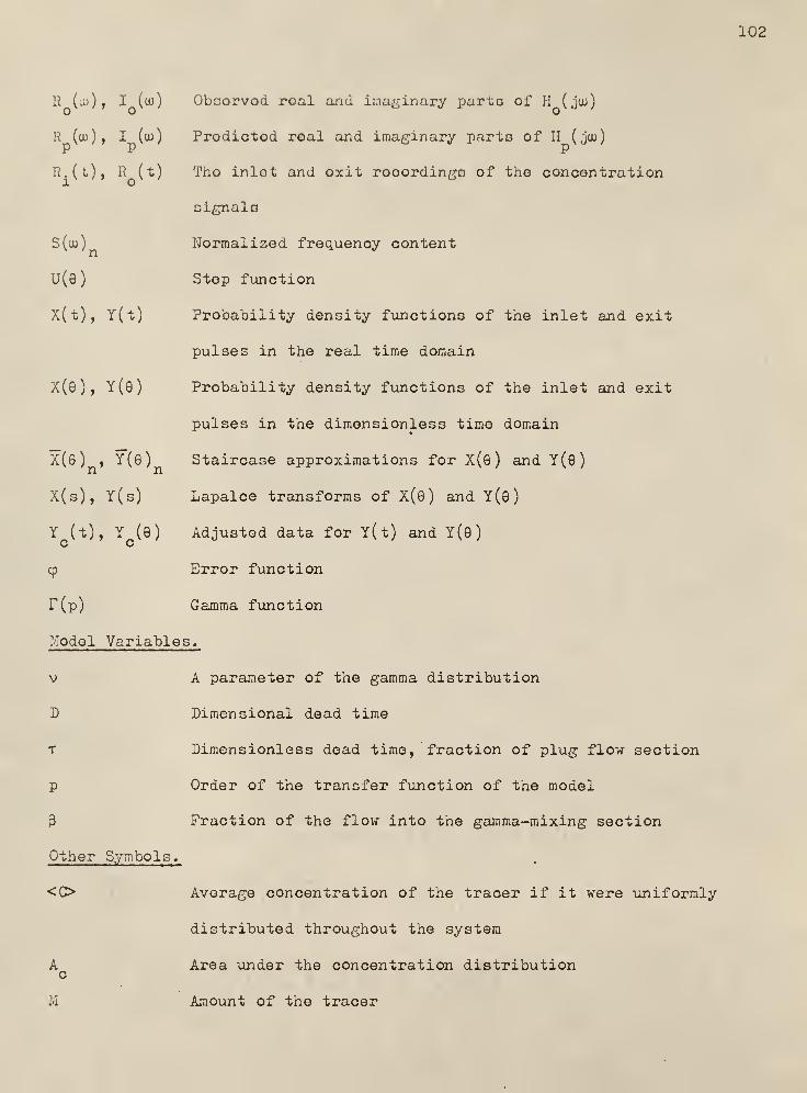
102
R (m) , I (to) Obsorvod roal arid imaginary parts of PI ( ju>)
R (uu), I (uo) Prodictod real and imaginary parts of II (juo)
R.(t), R (t) Tho inlot and exit rooordings of the concentration
signals
S(to) Normalized frequency content
U(e) Step function
X(t), Y(t) Probability density functions of the inlet and exit
pulses in the real time domain
X(8), Y(9) Probability density functions of the inlet and exit
pulses in the dimensionless time domain
X(e) , Y(q) Staircase approximations for X(9) and Y(B)
X(s), Y(s) Lapalce transforms of X(9) and Y(s)
Y (t), Y (9) Adjusted data for Y(t) and Y(e)c c
cp Error function
r(p) Gamma function
Model Variables.
v A parameter of the gamma distribution
D Dimensional dead time
t Dimensionless dead time, fraction of plug flow section
p Order of the transfer function of the model
3 Fraction of the flow into the gamma-mixing section
Other Symbols.
<0 Average concentration of the tracer if it were uniformly
distributed throughout the system
A Area under the concentration distributionc
M Amount of the tracer

103
V Fluid volumo containod »in tho systom
Q S toady flow rate
t, p, Mean residence timeX
K., K Proportionality factors in the inlet and exiti' e
concentration recordings
The kth moments of X(t) and Y(t)
The kth moments of X(9) and Y(g)
The means or the first moments of X(t) and Y(t)
The variances of X(t) and Y(t)
The skewnesses of X(t) and Y(t)
Difference between the means of Y(t) and X(t)
Difference between the variances of Y(t) and X(t)
Difference between the skewnesses of Y(t) and X(t)
The means or the first moments of X(6) and Y(q)
The variances of X(e) and Y(9)
The skewnessos of X(e) and Y(e)
Difference between the means of Y(Q) and X(Q )
Difference between the variances of Y(G) and X(9
)
Difference between the skewnesses of Y(9) and X(Q)
Correction factors
Some constants
Mean, variance and standard deviation of the distribution
of 3 in each method of response data analysis
mtxk'
m , ,
tyk
m9xk' 9yk
^tx' »ty
2 2atx'
aty
tx' ty
^ ty=c
Aa?tyx
tyx
^9x' ^Gy
2 2aGx'
aGy
a6x'
C'I,
A^9yx
ACT9
2
yx
**29yx
P, Q
.:, N, J
V V a3

104
u . cr . a Moan, varianco and standard deviation of tho distributionP P P
of p in oach method of response data analysis
Subscripts.
k kth
t Real time domain
9 Limensionless time domain
T Gamma-mixing property,
p Plug flow property, predicted property
o Observed property
T Total property
m By moments method of analysis
s
,
By s-plane analysis
f By frequency response analysis
x Inlet property
y Exit property

105
LITERATURE CITED
1. Danckwerts, P.V., Chem. Eng. Sci., 1_, 1 (1953).
2. Zwietering, Th.N., Chem. Eng. Soi., 11, 1 (1959).
3. Bischoff, K.B. and McCracken, E.A. , I&EC, ^8, ]_ (1966).
4. Hyman, D. and Corson, W.B., CEP, 61, _6 (1965).
5. Johnson, J.L., Ph.D. Dissertation, Kansas State University (1966).
6. Cha, L.C., Ph.D. Dissertation, Kansas State University (1965).
7. Hougen, J.O. and Walsh, R.A. , CEP Symp. Series, Proc. Dyn. andControl, 36, £7 (1961).
8. Otto, R.E. and Stout, L.E., JR., CEP Symp. Series, Proc. Dyn. andControl, 3ji, £7 (1961).
9. Williams, J. A., Bulletin SRC 60-C-64-22, Systems Research Center,Case Inst, of Tech. (1967).
10. Kendall, M.G., "The Advanced Theory of Statistics" Vol. I & II,
Griffin & Co., London (1947).
11. Churchill, R.V., "Operational Mathematics," McGraw-Hill BookCompany, Inc., New York (1958).
12. Stater, V.E., Ph. D. Dissertation, Illi. Inst, of Tech. (1963).
13. Rooze, J.W., Bulletin SRC 20-C-62-6, Systems Research Center,
-
Case, Inst, of Tech. (1962).
14. Aris, R., "Intracellular Transport," Academic Press Inc., NewYork (1966).
15. Ann, Y.K. , Ph.D. Dissertation, Kansas State University (1966).
16. Huss, C.R., and Donegan, J.J., MCA Tech. Note 3598 (1956).
17. Schnelle, K.B. and Clements, tf.C, Jr., "Pulse Testing for DynamicAnalysis," Vanderbilt University (1963).
18. Newton, G.C., Jr., Gould, L.A. and Kaiser, J.F., "AnalyticalDesign of Linear. Feedback Controls," John Wiley and Sons, Inc.,New York (1961).
19. Levenspiel, 0. and Bischoff, K.B., "Advances in Chemical Engineer-ing," Vol. 4 (1963).

106
20. Lav;, V.J. and Bailoy, R.V., Chom. Eng. Sci., 18, 189 (I963).
21. Fine, P. A. and Bankoff, S.G., I&EC, May (l%7).
22. Nakanishi, K., "Chemical Engineering Study of the Fluid Mixingin the Reactors," Japan (1967).
23. van der Laan, E.T., Chem. Eng. Sci., 2> i87 (1958).
24. Coughanowr, D.R. and Koppel, L.B., "Process Systems Analysis andControl," McGraw-Hill Book Company, Inc., New York (1965).
25. Shinsky, E.G., "Process Control Systems," McGraw-Hill BookCompany, Inc., New York (1967).
26. Roemer, M.H. and Durbin, L.D., I&EC Fundamentals, 6_, 1 (1967).
27. Adler, R.J., "Finite Stage Modeling," 4th National Chem. & Petro.Syrap. of the Inst. Soc. of America, April 9-10 (1962).
28. Hays, J.R., Clements, W.C., Jr. and Harris, T.R., A.I.Ch.E.Journal, March (1967).
29. Johnson, N.L. and Leone, F.C., "Statistics and ExperimentalDesign" Vol. 1, John Wiley & Sons, Inc., New York (1964).
30. Fan, L.T., "The Continuous Maximum Principle," John Wiley & Sons,Inc., New York (1966).

107
APPENDICES
COMPUTER PROGRAMS
( IBM 1410 )

108
TAPLF A-i FORTRAN PROGRAM FOR COMPUTING IMPULSE RESPONSE OFGDMWB.
IMPULSE RESPONSE OF GAMMA MIXER WITH BYPASSING BY Y S WU1 FORMAT ( I 3
)
2 F0RMATOF6.2 )
3 FCRN!AT(5H1TAU=»F4.2»5X,2HB=»F5.2»5X»2HP=»F6.2 )
4 FORMAT ( 14HL Z Y (Z )
)
5 F0RMAT(F6.2tF8.3)RFADU »1>Lnc iro m=i ,l& C AD( 1 ,?) T,R,PWRITE(3»3)T»BfPFP=1.NP = P
CO 10 J=l ,NPFJ = J
1C FP=FP*FJC= (B*P)** (P+l. ) /( l.-T )**P/FPA=P*B/ (l.-T)Z = T
V'RITF(3,4 )
DO 20 1=1 ,30ZT=Z-TY=C*ZT**(P-1. )*EXP(-A*ZT)WRITE(.3»5)Z»Y
20 Z=Z+0.100 CONTINUE
STOPEND

109
TABLE A-l-1. LIST OF IMPORTANT PROGRAM VARIABLES OF TABLE A-l.
Computer Designation.
L
T
B
P
FP
Z
ZT
Y
Comment: -> •
Number of runs to be processed
T
3
P
PJ
(3F)P+]
(1-t) P Pi
spl-T
G
e - t
Y(e), e:(e)

110
TAP! c A-2 FORTRANGDMWB.
PROGRAM FOR COMPUTING STFP PFSPONSF OF
1
15
16
1 °>
1 9
?0
STFP RESPONSE OF GDMWB BY NUMERICAL INTEGRATIONDIMFN5ICN F ( 30
)
FORMAT! 13
)
FORMAT (3E6.2 )
FCRMAT(bHlTAU=,E4.2,5X,2HB=,F5.2,5X,2HP=,F6.2)FORMAT ( 14HL Z Y(Z )
)
F0RM/\T(F6.2,F8.3)RFAD( 1 ,1 )
L
00 100 m=i ,l
PFAD( 1,2)T»B,PWPITF< 3»3)T»B»PA=P*p/ ( 1 .-T)D=R**(P+l.)*P**P/< l.-T)**PBl=l.-BZ=TNP=P-1
.
DZ=0.1FP=1.F(1.)=0-y -mIF(MP)15»15»9^0 1^ I=1,NPFI*IFP=FP*FIC=D*DZ/FPWRITE (3, 4 )
DO 20 J=2,26ZT=Z-TIF(NP) 18,18,16F( J)=ZT**(P-1- )*EXP(-A*ZT)AF=.5*(E( J)+F( J-l )
)
Y=Y+AF*CGO TO 19Y=n*(l./A-1./A*FXP(-A*ZT))+BlW*ITE(3»5 )Z,Yz=z+n.iCONTINUESTOPEND

Ill
TABLE A-2-1. LIST OV IMPORTANT PROGRAM VARIABLES OP TABLE A-2.
Comrutcr Desi/rnation. Comments.
L, T, B, P, A, Z, ZT See TABLE A-l-1.
D E 2_
(1-t) P
31 1-0
pp (p - i):
Y Y(9), F(0)

>-
CC<—I
<
X
112
coXo
C) *
a O _)
00 z <UJ M UJcc CO
CO CM X>- < • <t
u a NO *•
z > u_ XUJ CC * in10 II
•v
o X Q. OLU — X h-H
cc •—
.
CNJ t—
a. IS><<
O or ^Z UJ •* o>-< X CM <h- 1—
1
• 1^3 i. in X —
•
d U_ o o C^_ <; ^ •* UJ INI
O 5'II X o — -~ r-
u<
CDX
IT.
l_L^ , —
i
a O CNJ o _l ^ ^- #*
O UJ o 2 ^ ^~
u_(5
Xin
CCu_ < ^.
*t-
Ql
:f U_ » X V ^- «— in or< C\| 1 o r o~. z • 0.fy L_ • r» •» ^-. C) i
—
* w>
b C0 <f •—i X II CO — ^~ ^ i/ # 2O Z u_ o m 1—
(
\ *— —» V * — <or O •» »» e Q. Q. •—
•
>— «~ — —
i
»
a. CLCO C\J _^ _ II
< v£> _ • * cCN,
~yi s 1
c1
a* Cl _
z UJ ex (Nj ro < a • _j — o CL » >—
1
*— * * • • •—
•
a CC ^>-
< • Cr — »» • • t— _j <r •• j»! f—t • (— »— a 1— V- —
i
t—
(
c_ ^ rsl 3sc. rn 3 c-
vO r- 1—
1
X UJ .—
i
V ^ * _J 1— — •«-~ 2 —
-
>i< 1 1 w ~- + •—
•
* <—
h- 2 > ->»—
'
u_ u_ X o- _i Ul -~ — V ~ •> — <r 00 i^ * X m M rsj + 1 Cl a vO oCC s. ^ O CNJ c<- vO in l—l o v0 i—
<
c~ # »— r— fv » w #^ —1 X • * * X3 > a. «— o »> LL.
O Q Z >—
i
—« — <-~ -~ —
-
if «— •> «v r-H — II r t^ C^ c11— w. * l CL a * * * Zl. r\j r<^ X
U_ O u_, i/'. h- t— - t— »— < »- «—
i
I—
1
II i "J r— w* ^^ II 1 z. X — w •— X X c^ << — z~ 2 < < < < < X < — ^» t—
i
ii c — u_ Li_ 1— • < + >^ l/~. 7L * * a. 1- p- UJ •—
1
C LL 2 Z :> Z 2. 0" S. Q C o —
~
PSI c »- 1— O ^H I— • * () *— CC CO •— < in 1— I— a0" u -r- £K C£ 0: cc cr r- CC <- < f—
l
•—
•
< .— »~i ro —
'
< r—i >- u V) II II ii II ii—-
1
z: o c1 or »-i o CJ C, O O X O UJ LL a — C) U Ct CL C) II II V ii II II Cl <—
1
2 a o q: c> 1- 7.
«i u. C u. u. ll ll u_ m LL Q or c s c CL 2: 3- Q X rxi > X X) > a Cl <t N N ^; o CO u
U_ «—
1
CM (^ «d- co a* c o 3_i r— c^ t\
u

113
TABLE A-3-1. LIST OF IMPORTANT PROGRAM VARIABLES OF TABLE A-3.
Computer Desi^iation. .Comments.
L, T, B, P See TABLE A-l-1
K Number of frequencies to be usod
W(l) ith value of the frequency, tu.
, read in
rad./cec. but transformed to rad./unit
dimensionless time
PR Real part of H(juj) in equation (3-26)
PI Imaginary part of H(juj) in equation (3-26)
AM Amplitude ratio, given by equation (3-27)
ZR Phase angle in radians, given by equation (3-28)
ZB Phase angle in degrees

114
<
co
l— <lT. O0:—
.
0u_ V
>—
<
j} t—
z cOr—1 LU1— H-
Da. UJ:> l/.
C3 _J
u Da.
o:
5:U.
Q£T UL<-'
cOZ, I—O zCt OJQ iO
Z 2<Ct C*— Qia: •—
T
1
<
LU
COLU> <(X h-
D <U Q1— LUD cOQ. ZH- C)d aO cO
LU
OLJa:LU
— OC£
S >-u
OCt UJu_ ct<
cOh- 5:'*£. 5:LU
o z5T <C 2:ct z
t— ctLU
Z I
zu II
LU ~S
1/;
cO ZCt z—
• II
I—
I
Lu
z zLU LU2l ^O C)
>-
ozoLUCO
<N
OC)uLUCO
C\J
o
o-
vOON —i—
1
GO
r. c^
Ct ~cu CfD OO r\i
LU -Z II
O5 II
C) •— O>— cO •—
CO z cOz LU zLU 21 LU£ .— ^•—
1
O 1—
<
a
oCO
CO
zLU
o
LL — U_ — CO* <3" * <i" crn • 11 • —
.
C O Lu
Ll
TO0~>
oO <-!
rH LuU. *•
•> II
II
cO
LU
b^>_
QZOLUcO
>- Lu X
C)I/,
ct
COCt
O •—>-•-• X —Ct Lu
Ccr
U Xo zO
o ~LU CC. 2;H-. U> 5
vX
Z fVj ^ X<\J
o
Xom
11
cO
h-
LU
o->.
Cu
LU -^
»- w o-
z z •
Lu LU OZ Ct f-H
O UJ Lu
jj <ru •
2: oCT Lu
LU *Lu II
LU II Lu
Q LU
CtV LUX Lu X
U_ lTi —1
Z Ct C Lu
Xc
X
<r o <• Lu • Lu
< toi£ COCt LUf) .1
Z'
C/CT,
LU
C)
H UJ O
>— LU
zO LU
zLU —Ct (\j
y Ll1 •
X Lu O<T Lu Lu^ —> ^O •— r<"
a _jU. T•
9
II cf>
>—
LU' •^
1—< 11
cnu.
cr LUt— _l
< C^X X
1—
1
1—
«
LUr- a<r
• noc zLu X> <j-
1—
(
II#*
<r
LU •
1— v0
< LUCl m
e II
_^ <X —
c
1—
1
LU4- —I
— • O<r oc x• Lu x
CO •> 1—
1
r<
— <rc~. •
• vDCO LuLu »
11 •>
LU •
~i 00
C II
Lu' -*
Cr I— <rV X •
X 00<\j cr Lu
a.LU
LU C)5: X1—
1
r.
»- <ct: —• o
f\j •>
_l CuLU •—
•
O LU
_J C\J
LU LUQ 1-* <5: Ct
Z —
I
•> LUZ H-
_l z> <
a.LU
1
a
Lu_J
c>
QCt
UJI—
<cr
<Cr:
3 Ct
» r- n 00 o• — — u,
II ,-H 1— ^-. r-< w. ^<i U <a
5r" CO ~2
cr Ui ctO _l c>Lu Z Lu
> J:
Cr CtO C>Lu U.
<l X101-tt HiC) *Lu <f C
O O Q OUj C) LU Lu
cr d cr cr
Lu Ll
ct cr
«— rv r^ lf\ r-. \0 r^ cc c> c
<u u u

115
en**
J
co *
«— -^ • ue 2; CM *c #* # o
i—
i
I—
1
* •
II II u en•— 3 «~«
1 l
t r •—i *-» •—
•
-~ — — CO en»-i ~i < cc cr > (Tl >- >-
w Z •—
I
+ + + + > 5 S ;ri— >- X ^ to ~ i—i r\i <r CO 2 3 3 2.• — ~-- 9* * i— >- >- >- >- 3 tO to **
»- — .— o c O c c c c c r—
(
I—i — 2 5T 5 2 10 ^v V <—
<
^. vO sD II _J >- < CD 3 3 3 3 LU "V CNJ <r ii
c> #• •>_/ ..> i > o o c c c_ i—i LiJ # * * to CO tr u. 3 r-H >- >- 3
^ i—
i
.— ii II II II II II II II i—i l-H Q UJ U-i u. II II II n z > 2 5; <—
i
»•» »— ^- i—i (N. CO <r ^-< (X c <J~ 1 o 1 H :e 5 2 r-H CV c c<~ >—
1
2 Z> 1 Oo O > > > > X X X X z LO 1— UJ — —
i
*—
«
>- >- >- > h- 3 <J: tO 5. vO
<r < <; ^ |g >_ £ 51 2 5f *> II II 21 h- 1— h- 5. 2 5 s: i: 10 «— — II
l Ll. Lu _- 3 3 7s 2 3 * * 3 2 O —
1
— ii II II 3 _, 3 3 O II II II 5. C)< (T cr CO 00 i/) to 10 U~) to to 2; c 10 I— < cr: a tO lO lO tO O u a tO S. aU. c_i locr«r
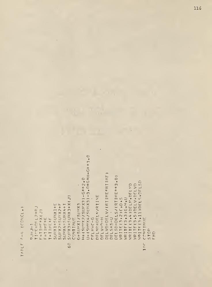
116
CO**
1
Li_ —O # ^: O• O •— • O
. CNJ * h- cn 10
* c a: * i. > _j
4 • * * _. u_O en LU LU lu u. Q—
.
1 1 LU 5: *> a •>
~) — -— ' 2i •—
1
—* l/) D »• • 1/
— Cn en .—
.
H- 1— •* » 2 > _lUJ u_ h- X CO. X X 1— q: CV Q X _j _i Lu
— -> + + + + X 5. cr — »— * *• Lu LU c• Ct — 1—
1
CNJ <f CO 5l _' ZI> X X X O O C; C —_J * —) X X X X _, L^ 1/. 2 > ' CO •— <-» »~ — 1—
1
u ex. —* T 5" 21 :> 1/ X V _' _l _l t\ 0-1 <f m t—
1
-<?i X LU u_ D D D id- Ll.' X CV <r O LU I Ll; 3 LU * *i »* e #> LU
c; LL * * # i/, i/) i/; la 1/ r—
1
X X 1 O 1 1 O CO, en CO en CO—
•
^ »— C u. LU LU n li ii ii *L X 5 5 L/ II <_" II *L~1 ii 2> Zz. ^> ^ Ox <t CO t—
1
:> ^_,""•,
11 C II II c Ll: L_ Lw, U. LL >—
>
—> Ll; >— — — X X X X 1— _ ,.- 1/ </ 2: 5T > > to 1/; (— 1— 1— \- »— h~ a*C~ II \ h- h- H— s. k. 5 "i^ z to «-. — _j _J _J _1 _J _j •—
•
•—
*
•—
•
»—
<
•—. 2i
~
)
*~> II II II 3 D _) 3-111 II 11 u. Ll. Ll. LU Lu Lu ex. a a CL Or C >- 2.
<r Cr I— Lu u. 1— lo «/) u" Co VJ O I 3 c O O O C. O JS. IS""-?
3» - O (/) Uj
LL c_J vO c.
<

117
TABLE A-4-1. LIST 0? IMPORTANT PROGRAM VARIABLES OF TABLE A-4.
Computer Designation.
L
kun
N
M
DELI
DSL 2
RTIME
RATE1
RATE2
WEIR
DIA
HOLES
DEPT
Y(D
X(I)
TIME
SUMY1
SUM2
SUMT4
SUMY3
C
B
S
Comments.
Number of runs to be processed
Run number
Number of values of the output pulse, Y(t)
Number of values of the input pulse, X(t)
Time increment used to read Y(t)
Time increment used to read X(t)
The mean residence time
Liquid flow rate
Vapor flow rate
Weir height
Hole diameter
Number of holes on tray
Measured liquid depth
ith value of output pulse, Y(t)
ith value of input pulse, X(t)
Time, t, sec.
EtY(t)
Et^t)
St 3Y(t)
SY(t)
Mean of Y(t), (j,
ty
Variance of Y(t), aty
Skewness of Y(t), a\" ty

118
TABLE A-4-1. (CCKT.)
Com^i tcr Designation
.
SUMX1
SUMX2
SUMX4
su:.:x3
G
H
U
del::
belmd
delv
DELVD
DELS
DELSD
Commentc.
stx(t)
Et2x(t)
Ft 3X(t)
EX(t)
Mean of X(t), m< tx
Variance of X(t), a
Skewness of X(t), o
tx
tx
^ty " ^tx
Ap,eyx
La
ty
2
tx
9yx
a, — o,ty tx
Aa9yx

119
\r> a.Q Q *O •~>
1 Q.X »— — * •
I— i/) — COu UJ CC #3
ICD*
> h- <r * CDc 7?
LU X ^^a
VCO ? c <r a —z< C) i—
<
• — •
ZF. 51 •* c \ «—
i
Q Z) i—
i
-~ +o >-
CO<1-
•
i—i
aLi. X X + *C) o co o_
Cl •
al/)
Xo
co•
*CL +
c (/; 1—
1
r- • * a^r" < ^ Li_ (Xi 0-< a 0_
X+a CO
*•
cr
cc
t—
(
*•
>+ CD
C\J
1
o X r*"i 1«— ^ —
z ^r c • <-* CD ^ CDi—
i
t— 1—
I
h- -^ V -— *k— i—
i
#> u_ Clj a —
»
• CD»— • 3e CD ^ * «— CO <r #—
• to •— I X a \ * l CLLi. — or CM -~ i—
i
<r w ^-~ CO *-» ~-
00 LU • CO • ** \ • * • V,CE >- X in •— X co D_ -• c—1 Q_ iH — —C _j •— Li_
#* o • •^ • + w-1 • a o
u. < 21 r\j 1—
t
p— CC r-i a «~ \ CO 1—
1
\ t- 1—1
^ > fy e- u_ «t + — Q. *- — + a o" •*
5 < < <r LU O #* U) a * * • * o_ a LL o< 5 • CO z X c *- • Q. 1—
1
c. — — 1— Vj
C C 5 O 5. <r »^ + CO * + * * i/ r •
o c; < IL D _l •v > • 1 CD 0. • • tr H- cC3 I a C\j -2 < CO o r-1 • •— ^* CO CO C Q < v< <r0: t- *• •—
•
•— »»1 c\ •^ * ^» «— •v \ + a o —*
Q. U. u. CO 2L" cr: #» 1— — -^ • • * * — — •— #• o^ i—i
*> O • D i— X #<: # * f\J C\J • • a. cc. a a CC # o
Z' m C£ vO 2! Z) • • * * CO CO o o li. "s. r o o< H- a u_ •—
i
_j #* Z) V C\j c^ * * * >l< * * * CD V Cxj o1l 2 «* «-» * X X _J _j V »— — * * — —
»
* * CL, Ll_ c C —
>
« •
1- LU CD CO en C\J '- .' X —
.
_J -~ CO vf * # 1— 1— <— ~ LL 1 i— in O c
q: 5. •— —
1
i
—
i
.—1 1—
<
i—
t
•< rsj t •* — <-«1 1 t— t— 1 CD CL i/; r (\i • •
1 LUC) o LD #* r—
I
> CO c~- H 1— • »1 1 CD li. o c CO ^> <j <} 1— _/
U- 5 Z h- t— h- h- h- .
—
II t— «— w1 1 i—
i
T-t • • O * * <: •— CO \ v. CD Q. I/: 2>— <L' < < < < •— >—
i
-* Li_ Lx • • w *— r-( f—
1
* c u. li U_ 1 c a D a. t—l LU >—
>
h- ? LI Zz. 2! y C o C »— I— r—
i
I—
1
1 1'— ^ a — ^- I— I— v: c o + + + 1— 1— D.
in h- a cr cc ,*v ct < <r <i ^-1 •—
i
t-^ ^- — II II II II u_ 11 II u~. KM — II n CJ 0_ ^ •~~ 21 O Q1 -i C) O O O O Lu C; IX. CL Ct II II II a cc D_ CD II G a u. Oi u_ CC a II II II li. O I— 2:
< u_ Li_ Li- li. Ll li- Cr: C cr ~s - 2* li- O u_ Ll_ C) o O O c t— ^_
"-" c o CO 0- V •- U CO Lu
L. (H es, co <r m C c o t_J ?—
i
r\ CO <rC«:
u
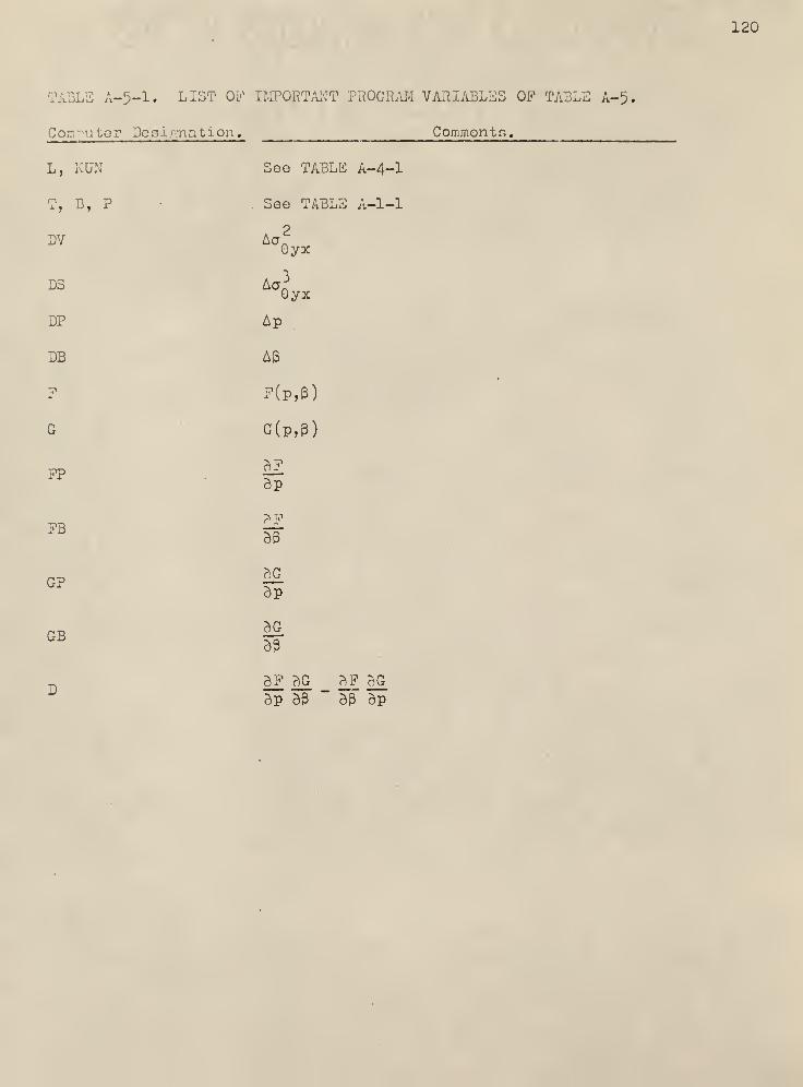
120
LE A-5-1. LIST Ob1 IMPORTANT PROGRAM VARIABLES OF TABLE A-5.
Co~ uior DoG.i.';nation. Comments.
L, KUN
m B, P
DV
D3
DP
DB
P
G
p?
PB
GP
GB
See TABLE A-4-1
See TABLE A-l-1
Aofl
2
yx
Ap
A3
F(pfp)
c(p,e)
SFBp
S3
SGSP
dGS3
M ££ <!£ ££Sp S3 ~ S3 Sp

121
z r-< zI UJ
Du
DCL
CO _Ju_ X
II CO
Uj -(j~: C)Z •-•
G r—a <l
i/) 5l
Lli i—or Xo
>- cc^ az o_Lw <o
fV _JU_ OG <Z OC•—
<
<t— aX —
-
CI
> <G i—
O <o
Cl
G gLL z2F i—<. aOr. u.c r-oCC U_Cl ^
_J;•-• ZD< Cl.
Cr
i— •2
or: GG cru. U_
<;
in
fV
UJGOT.UJ>C)z
ISJ o'—
•
o_J —I< _
CC XG *z —G
X OO co
X —I— r-t
LL >
Ll! Ol/) O< Hu —or x»—i c
< ~i— o</> o
colj —tO > *-
z * r v
G — •
C DcO co u_
Uj — c^OT ~2- •>
CO —U_ vD
zoXf-
Xi- r-< •*
or. >or
x
g
<x
• CO» reCO r-l
>- Z •— UJU G c^ cp22 •—
•w «—
LU l/) »— I—DZ <G UJ
r- xu_ CM
oo <X »-
r- x•> oo *UJ x
S <-h LUo. ccX XO <rf
r r
X Xr- LP,
>-
Uz gUj Uj
x cGLl uor _iu_ o
2
X uj ••
O r-< ll
CC ccu_ </)
a or lu
<UJa:<xCM
00
UJ>ccX
XCLzr
UlD
< C)X X
• o• o
00 zU. X• <f
II •>
<rUJ •
I—
cc
G_J
X -«
a
•c — UJX a — or ~-
•m • — r\j
r-i \0 CO •» i—. •—
•s
X Ll Cv U.m co — vO
X -*
iTl r-t
CM UJ
II
<
•- UJ<r _i
D —
x <?-
X •
r-i CO —r-i u_ v:» . •* . *
<r co i-t
• —
i
n
00 •> ~)
u_ <r —
L0UJCr
Xrvi
it
vO —U. ~)
i— >3" "d- » — •>
X • • V. Ii: r->
00 CO -~ *- II
Ql U. U_ <-• -~ -J
aUJc
U. LU
"- GI- X•> <rv —
i
_J C.U: •c a:•^ •—
#
r—
i
U_i
—I ISLl. *C (NJ
U.? I—Jli <« a:z .»
Z' •—
•
»• LUZ »-
X <V cc
— o
CLUJc10
GX
zr\i c^ii ii
—
i
~)— ~)•» •
-) ^
(Nj
UJI—<
UJ
<
UJ
> x
CO c^
< < <
UJ cc ccCC — G Ou. Q u. u.
or Or
G GU. Ll.
< < «C <
a < Cr Or. CCG Or G G GU_ U. U_ U_
i—i cx o" a", r-
— * — UJ w * •I- h 3 II h H rl C<II<X <«-~vCCr: LU CrT i-t X CC < <G > G » G fi b- GLLCrU-NfClLQ-D c
i—
i
<—I C\J
c^ it. r— o
X z t-v D Cr~- v —r-i — r-i—
i
in «—
<
** •* r»
Cm co c<^
r-t i-i +
c c z >:
<.<.!! II
L. LU 2 5.
Cc. or z 2.
+ <—< r—I •— — —-Ll Ll Ll
a c< <Ll Llcn cr
or: cc cc
cc
w

122
C\l <\J
+
>-
I
XI
>- .—
1
X /—1
< >- < XLu * Lu *a' o: O >-
< • < • <r
\ 00 \ 00 U-'
LU + UJ + •' ce^7 — ^. '— <•—
<
t—
1
•—1 <—
•
»
«-» 1- 1— t— 1 X
2: — >- 2' q: 1 ^~ 21 ~> X >L Ql ;~> <
2 •—> s Z" * 21 »—
«
i. ~) ~ - 5. * 2 -) LU2: *-* z> 2 "~* 2 ** 2. *"* D *^ 2 **"
— co >- * r ^~ c" >- CO X * ro "1 cc X — >—
4
• II + r— 11~~ 11 * II + 0. 11
>—II * IT. — 11
t- <—
.
>- _J — t-H >— -> X _j ~) <—
1
~) ^H r^ -)
z: o r\ — 2^ LU •—
»
>- t—
1
•—1 • r^ ~) 2* UJ -) X 1—
1
-J • * •• •—
•
c • •l
~C; II 1 m 1 D O II 1 Ln c m
^ c e 2"0 <j. 11 c — ^ c 0. ~— Sl to 11 O -~ %«£ C r\ •— cc CO ^» — O«—
II n z: 11 >- in •— 2 c 1 II 2 n X m ~J 2 c 1 11 I 1 u. u_ <r V. C c c>- X 11 f\j >- < f\ >—
1
II co 1—1 •-•II m X < in -)
11 vO -> —
•
2r 2 1— Ho 5: z- z 21 UJ ~
.
>-. — 1; 2 u_ «-- _J -> —j 2 2» CM >—
•
3 O1 _J Z> 2. 3 or O t—
t
2 II~- 2 C) D a C3 1—
1
^. C) 11•—
II II rr a C) 11 II II II
< l/) \S) ^ i/ < O >- 2. c •""• > 5 O tO < O X 2 ~> X ^ 2 ^ 2 O <. CO u c_
L C c c c O_' c If c m ccc- cv <\j CO in m >c<

123
zC;
vO
<.
Llj
_•
a
i CNJ CNJ
2?C 3 h-
# * 2--~ r—
I
•-» cnj C)CNJ _J CNJ _J ujs: Lli s UJ *•
* uj * Q —1
i—
i
* rvi * Lu_J — _i -— aLu • LU • #•
Q i—
i
Q i—i'
cr>:<
1 * 1 Lu«-» «—
i
^~ 3 a• CO • CO #•
i
*•
i—
i
1•
(M_l
*—
<
(XI 3 CNJ oi/) — cO —
•
z* — # «— <• Z • z f
r\j •—
.
CNJ 1—1 1—1
^~ CO — CO _Jv- * — * aCO — CO —
*
ip zO CM C) r\J • <U "5 O 2s * *
* * * # # CD— t—< »— CVJ — »—
•
<\i _l CNJ _l •—1 1—
^ Lu ^ Lu Lu <* c * Q CL »—
<
Cur— -~ (X ~— * LU r-
_J z _l Z — !-( D. mLU 1—1 LL; i—< LU — -J #^ 3a CO Q CO CL Cr 13 DC #i
>— * ~^ * + 3 z Lu —~» zr i-H z: i-H
4Cn s < m C. 3
~3 ~- ^ >—
•
s c Lu — * • #* >—
i
—
i
CO # CO # * 5. T a 3 ^c * m ——• • —»
4L * ^~ ? * — Q o O * — o * 3 S3 cm is * <—
i
»—
1
» t-* ~) + Q U z. z-
a: 2: rv 2_ <— -*— v. * i—
1
7r *~ i—
i
y: — U * * UJ Lu Lu < • () CNJ o— —* LU II # > ii * X * DD Cu o Cs CL h- r~ ^_' •* ri ^^"+z 3 ^ 1—
H
—
-
^ 3 -*>i< u + 1
v. \ — < ir> LU OsJ CO 3\ •-« •-« •—
i
^-i • 1—1 3 1—1 • .—
1
II C c a: •—
i
II II ii Q «— w Z.• — H- o w < 1—
•
a c •~~ c i—
i
o r~> * # _ 3 o r-
1
tv, II LU LU l—
c
f\l 3: cr CNJ — >- + + + c^ 3 X + + + O < < ii ii fl -J _j f- H- H- 1— CuII it ii II II < II CQ II II u ii a *L II II Ol — 1— CI O "Z. -< i—i z: o Q
•—
1
r\j o~ o —' r—( II r-' II C) 3 1—
1
II i—i II LU C. •-• ij_ Lu <L «z z c; LL Cu o »— z:3 **-^ a CO < < cc cc
c
o cO u u o ocCO
O 3 3 a a. or. < < u 3 2OuoNO
Ifl Lu
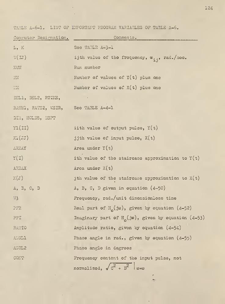
124
A-6-1. LIST OF
Computer Designation.
L, K
'(U)
KUH
DELI, DEL2, RTIME,
RATE1, RATE2, WEIR,
DIA., HOLES, D3PT
Y1(II)
XI (JJ)
AREAY
Y(I)
AREAX
x(J)
A, B, C, D
*0
PPR
PPI
RATIO
ANGL1
AITGL2
CONT
IMPORTANT PROGRAM VARIABLES OF TABLE A-6.
Comments.
Sec TABLE A-3-1
ijth value of the frequency, uu . . , rad./soc.
Run number
Number of values of Y(t) plus one
Number of values of X(t) plus one
See TABLE A-4-1
iith value of output pulse, Y(t)
jjth value of input pulse, X(t)
Area under Y(t)
ith value of the staircase approximation to Y(t)
Area under X(t)
jth value of the staircase approximation to X(t)
A, B, C, D given in equation (4-50)
Frequency, rad./unit dimensionless time
Real part of H (jco), given by equation (4-52)
Imaginary part of H (jcu), given by equation (4-53)
Amplitude ratio, given by equation (4-54)
Phase angle in rad.,given by equation (4-55)
Phase angle in degrees
Frequency content of the input pulse, not
/~2 2~I
normalized, V C + D I to=cu

125
>-
cc
CD
a
Lu
O
<33
cO
H- I/)
(— >— <U_ «il
<oro LLll. CO
>" O< Q.ct COo UJO ctcc
0. >u
z 2:<. luQl Z>(— Qct LU
o OHLu u_
r-
<LL
i
cc<
U, *•
X >Q C\J (VO -« 1—
I
<I C\J #> Z1— <\J X —LU — c — o51 Q r—
1
•<5
• r* (— o i—
.
l/j -~ I/; i-H XLU c\j Lu UJ c*cc (NJ I-
I X• c: <t (NJ oo INI «v 1—
(
1—
1
LU •v X ** w
cc — o <r _lu_ (NJ
(Nl
1—1 •
c<LU
> — X •—I DiCO<
< UJ X
c r. I X ^
z — co <r X•—
•
CVJ ** * mcO INI X m #•
oO — c- • C)< i—
•
1—
1
r- >—
1
Q. Li_
0.Lu
"-^-
> — r X Di33 f\J
(N
i—i
O ^^ a
X -^ X ro < CO Zf— ct o • 5 i—
•
•^
1 . Li. 1—
1
r- X -~ * i—i
!£ #* 9*
cc
LL. L9LU
II
oII
ct (Ni I X X a UJ •*
LU (NJ — r—
1
<f Lf\ 1— —X — CO #> w* •^ LU 1— •—
<
1—
1
•—
•
»—
<
X CO G _J 1—
«
^^
51 C) #>
,_,
• LU u_
< — or « a_ u_ <r O •^
5T (NJ LU C) •^ X LU -~
2L CNI CC z X _J o ct: •—
< — — 5 <r .^ » LU ^>
L3 ccO
C\j
•X>z
_J< CO a
Xin U_
ct
Ll. #> iTi 1—
i
i—
i
•» C) •*
O(NJ
Ll<N2
vOCl1— X < vO C) *
0.-^> 1—
1
0. (NJ •^ or • — vO or • ^L 2T ai X — z~ -— cc «—
i
CO _J Ct' r> _j <r _l 3 #^ V 2; »»^ yz •— en • X 1— X o —I i LU i—i X _J _j V I— <-» ^ o —CO Z CO — co (N LU c CV X -t _l LU o —
.
•> — *~ <r ^-« 1—
1
v0
C) M (N Ll r J co 1—1 q: l—< rH lD O 1—* i—
1
r—
t
(NJ cc, * m # p
o •* II•* r cc. •> CO CO
z to (— 1— h- h- h- - t— 1— < (— t— i-H ~) «—
i
r—
1
— r— ^» —
'
• • • •
1—
(
2 < < < < <• < LU < < ^_ < < «— o — w Lu — LU LU • • • o o O eK— lu' J. i_ s: 5: s~ 5 Ct ^: "Z. a >' 5" Q o c o 1— c (— h- o O o II II II ii
(— i> QC Ct cc q: ct or < ct cc •< a Ct < 1—1 <l < •—
.
<. 1-1 i— i—
i
II ll II cc, a LL a-< >—
>
O O O O c. O D c> C; X o o LU C) LL Lu Lu ll Ct CK Lu L^ o Ll u_ o LSu. Cj u_
.—
i
fN
Ll
CO
ll Ll Lu Gi—
i
LL
00
LL.
c-
Ll.
or-t
a c or Od Ji or ^ .^ IS LO
o10 c0 l0 00 CO CO
u

N N> >-
N Ncc cc
126
O
i
<UJ
CO ~"N C— >-—- -it.
CC X>- ** XCC W+ X>- *— 0.* 1
X —* c.X X*< *
CD Cl X XN, N 1 *CC 0. >- XN. N. V ^> > c a
«— ~+ N N. * +
,_ i—
i
>- >-
N~ Q.CC X
~— —
>
—
•
•—
i
X V3^ 2j iT\ —
-
— — »c X* * • >- > >- > X *I- 1— >* + N + — * X«— ~ * CO > a O X VLO z ^ >- V, >- C) + a.CO -I —
.
^~ * CC * _J cc *CD — ~ <^/ to Q_ — —
•
CO *N a < ~r •
\ ~ .— * * * CC — — -~ — * ^ CNa <—i •—i — — »-m a. C£ >!< a >^ X X +"s -^ — a CO 0_ v. INI X > X >- * — * X-~ 2^ 3 1 1 + -< * 1 * i "N in Q. *- X ^•— -~ * * • • CC a vO CO X O. CO • INI a * X«— Q. t- t— f—
1
<—
t
Q. — CT X i X *«v l * IN • *3: »-» # 1 1
—
»
— >;< ST <\j CC a * a. * X >- DQ a If. <\ X7* * I lT\ inj in + 1 cc < • X X CO X a. V N IN + X a ^^ ^,* —
1 I • * * X) > or •—
i
a. K- r- * * > >- * >!< >!' X X * INI M + — *r~* H ~ # 1 c_ Q. * # a Q. — <. lTi CO a X X N V. >- > >- >!< # a «— * IN * >•
II 1 ^ X ~- — — X X n II ii 11 ii N. \ * * a. a — — — ","~ X >^ * a ^- Q. «~•—
'
• < + * t/: Z * * <-- -» -~ <~ » I X • • -T- X II II II # * > > * * II li
o r— t- • * (5 — CC CO •—
•
— i—
i
•—
i
—1 i C\J r\j T i rx a tNj Cl _t_ i 1 X X CN C.
00 -~ < i—i >- u if) II II II ii II ii ii ii CO CO Q. II II ii II ii II CO CO'
o li II II II II II Ct •—
•
a •-4 2 cr c CO Q tj a CO Q_ (\j rsj (\i QD 0. D a c a <M (N
Q X N >- X X> > Q_ a. u_ Li_ < rsj INI X X >- > N N IN IN INi X X Z> D > > X X
CO<

CL
*X+
127
oo<*
O
I
<
Ll
_JCC
a' aX CD— CM CM —
«
* a X CM »-«
iTV CM * CO a•
1
X*X+
CM>
COCM
> X Jj * >V * X X >!<
>- -f) * + X CM a a C\J
\ + a CM + CO CO CO a-^ CM X LO LO >—
>
1—
1
»—
•
>-H
a Q w» CM > a a a a> »-~ CM * X # * * * *# CM «— — — X CO * a o o o C)X Q. CM «» «— >:< + > X a a a a* CM a >—
<
.—
!
D — —• >— + »-« •—
•
—- i—
.
i—
i
X INI CM «— — =(< a CM * a CM Q Q Q QV —» * IN jj£ !3 CC CC a CO CC. O + + + +X a CL * * * + C J CM + CM CM a a a a
1 CE + a h- 1— —
-
X _J *» X > •—
>
i—
<
—• —i
-~ CM Cl Q + — CO >:< * CO >fc >!< a a a aQ_ inI rN CD a to z X X X X > X >!< * * >;< oX ¥ * CM IN o •— * + + * + + CO a CC o aW > • IN * u I/) CO CC CM CC CC CMX — * CM * •
1 + X X Q > X a a a a a Q# CM a — — X CM .re CO A >;< CM * * CM + + + + 3,<
T* CD + * CM >!< »-« X > CO a X CO a X CM CL a CM C)+ CM a: > a a. !f< * * + X * + > # CL a CO CC co a a"
fsi PsJ 1 CM + x X X CO — X CC — > t— —
i
a r a a —>
X * * — M CC + # — * »— X * + > * + a a a a a a Q* > > a * INI — CC a CO Cl * CO a >i< CC a * * * # * * +X + + rN __ * a + X + > X + X X + X o o o C) o C) C)* i a >)c + ) fN CO * CO * + a * + a >i< a a a a a r> rv
x > rsj a CC + * X X X X CO X a CO > a «-» —
«
•— i—
(
a a a a a* * * + ISI CC a * + # + X >w X X >;< > — »—
i
Q Q Q /•> X Q Q• CL, Q. (N * INI + X a > a * X * >!< X * -^ — + + + + + + *
cm INI > •-« CO * rN * x * X X + • > + • a •—
•
CC a CO re a a C)w — * X< _J a —
-
Q 1 * CO * »— a CM — a CM C) C3 Cl o- a a a a a# * 0. a —- ~T\
>;< + X + > * X w »!< X —1 1 a a a a a a a
>• a ~ > * * 0. _) — ^> — • * >'.< « * * a •—I >;< >c * * * * o u «.,
—i 1 i a a X * * * * (Ml _j a, CM > (1 1 Q. a C) a Q'J a U) a + + +
II n II n ii n II X .i. X c II ii n II ii II ii ii a a a a a a U J a IXCM <N Q. CM <M a CM II ii II II CM a CM CM a CM C) C) a a a a a a to tO toCL CO CC CL CL a: a a' a CD a CO 00 a CO CO a a a c a ii ii ii ii II ii II
CM CM <M CM CM CM CM a a •—
I
»—
«
a a a •—
<
•—
i
»—
i
a »—
.
ii ii CO 0. en a a' a oX D X X > > ~> a a a a a a a a a a c, a a o u. u. o o i/) o", f;
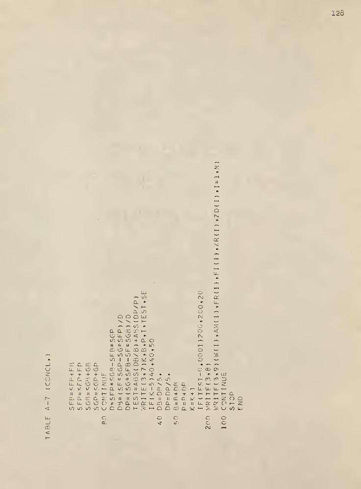
128
Q
CT
UZOu
1
<
CD<
LU ^«—
«
tO (N CKa # •* U_\ f— *
ex cO O •—
Q Q UJ CNJ «\ \ W h- 9> —
«» to O 210. 0_ cc cc h- O <
U_ < » CM #*
to to to + a »- —* * * — «v ii^ 1—
1
•—
cc to lo- co CO •* O ^u_ to tO \ •* O *^
to 1 1 cc v: ^ O «—
CD CL cc a 1 Q. CO a — # • — —
«
Li_ Ll cf: O u_ — r- O c a O+ + + + u_ O to tO to #* c • •
1» 9* UJ
cc c 2L" a. 2^ 0', V # D m -— \S\ LP. t— CO Du_ u_ 13 2: * Ll < — lO V. V, cc a t/\ —
»
— z0' I/. LA I/. ^~ a to to II UJ 1 a. a c c t LU Ll, u_ ~^
11 II II II t— LL. «-» w. 1— I— v: a + + + 1— t— h- 1— a.CD a. Lt: a 2 to II II LO •—
•
>—11 n cc a ^ -~ >—
1
•—
1
zLl u_ C c it an a UJ ct u_ en a II 11 II u_ o: tr i—10 tO cO to
c
Cl <2l 1— 25 »—
•
>3"
a, CO
c.
in
Q. V —
«
3i
cex
i£ u
1—
1
10

129
TABLE A-7-1. LIST OF IMPORTANT PROGRAM VARIABLES OF TABLE A-7.
Computer Designation. Comments.
L, Kli See TABLE A-6-1
N Number of frequencies to be fitted
T, B, P See TABLE A-l-1
T
>'[(l) ith value of frequency, rad./unit dimensionless
time
OR(l) Observed real part of H (jcu)
Ol(l) Observed imaginary part of H (jcu)
DP, LB Ap, A3, given by equations (4-75), (4-76)
H, Y, X, Z, U, V See Chapter 4, page 76
PR RP
PI I
HB
HP
YB
Y?
Z3
Z?
Z2B2
Z2BP
Z2P2
P
bb
MSp
SY
S3
BYBp
£ZBB
BZdp
a2z
as2
a2z
BB^p
Z
2
a2z
op

130
,B A-7-1. (CONT.)
Cor.outcr Doci/p-.ation. Cor-monts.
X3
XP
U3
UP
V3
VP
X232
X2BP
X2P2
U2B2
U2BP
U2P2
V2B2
V23P
V2P2
Map
Msp
5US3
Bp
SVS3
SP
afx
B32
*2X
SSSp
32X
8P2
a2u
S32
,2u
333p
a2u
3P2
32V
3?2
a2v
A33p
ap2
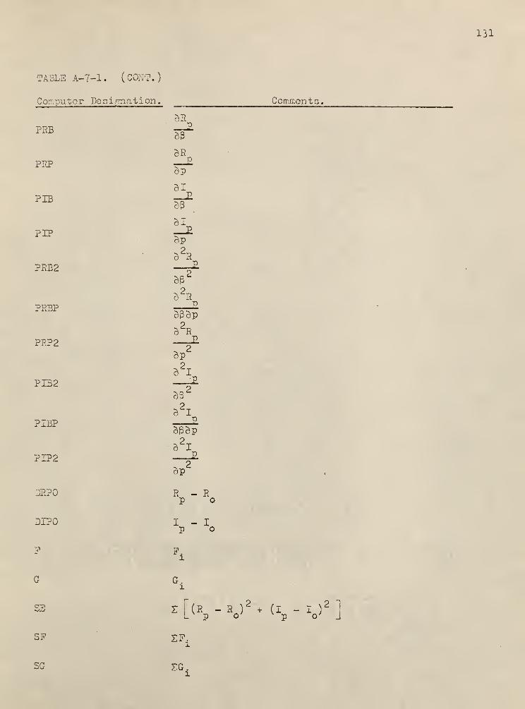
131
TABLE A-7-1. (CONT.)
Computer Desi-'rnation.
PRB
PEP
PIB
PIP
PRB2
PRBP
PRP2
PI32
PIBP
PIP2
DRPO
DIPO
F
G
SE
SF
SG
Comments.
BR—
E
B3
BRp
Bp
51
B3
31_EBp
B2R
ae2
2BRp
B3Bp
o xi
P
BP2
B2IP
B32
B2Ip
B3Bp
B2IP
Bp"
R - RP o
I - IP o
- n2S (R .- R ) + (I - I )L p o K-p o J
SF
FG

132
. JLE A-7-1. (CONCL.)
Computer Designation.
F3
PP
GB
G?
S?B
SFP
SG3
SG?
D
K
91
S3"
dF,i
Sp
SG.i
S3
SG.l
Sp
Z
2
Z
SP.
Sp
SG.i
S3
SG.i
Sp
SF,
Common ts.
SG. SF. SG.
Z— Z— - Z—- Z—^Sp ^S3 ^S3 Sp
A6_ Ap_j
P i
Number of iterations
MODEL PITTING AND METHODS OP RESPONSEDATA ANALYSIS POP, LIQUID MIXING ON
DISTILLATION TRAYS
by
YIE-SHON WU
B.S., NATIONAL TAIWAN UNIVERSITY, TAIWAN, CHINA, 1963
AN ABSTRACT OP A MASTER'S THESIS
submitted in partial fulfillment of therequirements for the degree
MASTER OP SCIENCE
DEPARTMENT OP CHEMICAL ENGINEERING
KANSAS STATS UNIVERSITY
Manhattan, Kansas
1968

The experimental data previously obtained by Johnson in his
investigation of liquid mixing on distillation trays were analyzed
by two other methods of response data analysis, i.e. the moments method
of analysis and the frequency response analysis. The same gamma
distribution model with bypassing (GDMWB) was again fitted. The
resulting parameters in the model fitted by these tivo methods were
compared to the results given in the s-plane analysis by Johnson. In
conclusion, the purpose is to obtain what appears to be a rapid,
reliable and simple procedure for procuring information about a flow
pattern of liquid mixing on distillation trays.