model order selection - sal€¦ · model order selection as a hypothesis testing problem, with the...

IEEE SIGNAL PROCESSING MAGAZINE36 JULY 20041053-5888/04/$20.00©2004IEEE

he parametric (or model-based) methods ofsignal processing often require not only theestimation of a vector of real-valued param-eters but also the selection of one or several

integer-valued parameters that are equally importantfor the specification of a data model. Examples of theseinteger-valued parameters of the model include theorders of an autoregressive moving average model, thenumber of sinusoidal components in a sinusoids-in-noise signal, and the number ofsource signals impinging on asensor array. In each of thesecases, the integer-valued parame-ters determine the dimension ofthe parameter vector of the data model, and they mustbe estimated from the data.

In what follows we will use the following symbols:

y = the vector of available data (of size N )θ = the (real-valued) parameter vector n = the dimension of θ .

For short, we will refer to n as the model order,

even though sometimes n is not really an order (see,e.g., the above examples). We assume that both y andθ are real valued

y ∈ RN

θ ∈ Rn.

Whenever we need to emphasize that the number ofelements in θ is n, we will use the notation θn . Amethod that estimates n from the data vector y will be

called an order-selection rule.Note that the need for estimatinga model order is typical of theparametric approaches to signalprocessing. The nonparametric

methods do not have such a requirement.The literature on order selection is as considerable as

that on (real-valued) parameter estimation (see, e.g.,[1]–[7] and the references therein). However, manyorder-selection rules are tied to specific parameter esti-mation methods, and, hence, their applicability is ratherlimited. Here we will concentrate on order-selectionrules that are associated with the maximum likelihoodmethod (MLM) of parameter estimation. The MLM is

A review of information criterion rules

TPetre Stoica and Yngve Selén

©A

RT

VIL

LE

likely the most commonly used parameter estimationmethod. Consequently, the order-estimation rules thatcan be used with the MLM are of quite general interest.

Maximum LikelihoodParameter EstimationIn this section, we review briefly the MLM of parame-ter estimation and some of its main properties that areof interest in this article. Let

p(y , θ) = the probability density function (PDF)of the data vector y , which depends on theparameter vector θ , also called the likelihoodfunction.

The maximum likelihood (ML) estimate of θ , whichwe denote by θ , is given by the maximizer of p(y , θ);see, e.g., [2], [8]–[15]. Alternatively, as ln (·) is amonotonically increasing function

θ = arg maxθ

ln p(y , θ). (1)

Under the Gaussian data assumption, the MLM typical-ly reduces to the nonlinear least-squares (NLS) methodof parameter estimation. To illustrate this fact, let usassume that the observation vector y can be written as

y = µ(γ ) + e (2)

where e is a (real-valued) Gaussian white-noise vectorwith mean zero and covariance matrix given byE {ee T } = σ 2I , γ is an unknown parameter vector, andµ(γ ) is a deterministic function of γ . It follows readilyfrom (2) that

p(y , θ) = 1(2π)N /2(σ 2)N /2 e− ||y−µ(γ )||2

2σ2 (3)

where

θ =[ γ

σ 2

]. (4)

We deduce from (3) that

−2 ln p(y , θ) = N ln 2π +N ln σ 2 + ||y − µ(γ )||2σ 2 . (5)

A simple calculation based on (5) shows that the MLestimates of γ and σ 2 are given by

γ = arg minγ

||y − µ(γ )||2 (6)

σ 2 = 1N

||y − µ(γ )||2. (7)

The corresponding value of the likelihood function isgiven by

−2 ln p(y , θ

) = constant +N ln σ 2. (8)

As can be seen from (6), in the present case the MLMindeed reduces to the NLS.

A special case of (2), which we will address in thisarticle, is the sinusoidal signal model

yc (t ) =nc∑

k=1

αke i(ωk t+ϕk) + e (t ), t = 1, . . . ,Ns (9)

where {[αk ωk ϕk]} denote the amplitude, frequency,and phase of the kth sinusoidal component; Ns isthe number of observed complex-valued samples;nc is the number of sinusoidal components presentin the signal; and e (t ) is the observation noise. Inthis case

N = 2Ns (10)

n = 3nc + 1. (11)

We will use the sinusoidal signal model in (9) as a vehi-cle for illustrating how the various general order-selec-tion rules presented in what follows should be used in aspecific situation.

Next, we note that under regularity conditions, thePDF of the ML estimate θ converges, as N → ∞, to aGaussian PDF with mean θ and covariance equal to theCramér-Rao bound (CRB) matrix (see, e.g., [2], [16]for a discussion about the CRB). Consequently, asymp-totically in N , the PDF of θ is given by

p(θ) = 1

(2π)n/2| J −1|1/2 e− 12

(θ−θ

)TJ(θ−θ

)(12)

where

J = −E{

∂2 ln p(y , θ)

∂θ ∂θT

}(13)

is the so-called (Fisher) information matrix.Note: To simplify the notation, we use the symbol θ

for both the true parameter vector and the parametervector viewed as an unknown variable. The exact mean-ing of θ should be clear from the context.

The “regularity conditions” referred to aboverequire that n is not a function of N and, hence, thatthe ratio between the number of unknown parametersand the number of observations tends to zero asN → ∞. This is true for most parametric signal pro-cessing problems but not for all (see, e.g., [17]–[19]).

To close this section, we note that under mild con-ditions

[− 1

N∂2 ln p(y , θ)

∂θ ∂θT − 1N

J]

→ 0 as N → ∞. (14)

To motivate (14) for the fairly general data model in(2), we can argue as follows. Let us rewrite the nega-tive log-likelihood function associated with (2) as[see (5)]

IEEE SIGNAL PROCESSING MAGAZINEJULY 2004 37

− ln p(y , θ) = constant + N2

ln σ 2

+ 12σ 2

N∑t=1

[yt − µt (γ )

]2(15)

where the subindex t denotes the t th component.From (15) we obtain by a simple calculation:

−∂ ln p(y , θ)

∂θ=

− 1σ 2

N∑t=1

[yt − µt (γ )]µ′t (γ )

N2σ 2 − 1

2σ 4

N∑t=1

[yt − µt (γ )]2

(16)

where

µ′t (γ ) = ∂µt (γ )

∂γ. (17)

Differentiating (16) once again gives (18) (shown atthe bottom of the page) where et = yt − µt (γ ) and

µ′′t (γ ) = ∂2µt (γ )

∂γ ∂γ T . (19)

Taking the expectation of (18) and dividing by N , weget

1N

J = 1

σ 2

(1

N

N∑t=1

µ′t (γ )µ′T

t (γ )

)0

0 12σ 4

. (20)

We assume that µ(γ ) is such that the above matrix hasa finite limit as N → ∞. Under this assumption, andthe previously made assumption on e , we can also showfrom (18) that

− 1N

∂2 ln p(y , θ)

∂θ ∂θT

converges (as N → ∞) to the right side of (20), whichconcludes the motivation of (14). Letting

J = − ∂2 ln p(y , θ)

∂θ ∂θT

∣∣∣∣θ=θ

(21)

we deduce from (14), (20), and the consistency of θthat, for sufficiently large values of N ,

1N

J ≈ 1N

J = O(1). (22)

Hereafter, ≈ denotes an asymptotic (approximate)equality in which the higher-order terms have beenneglected and O(1) denotes a term that tends to a con-stant as N → ∞.

Interestingly enough, the assumption that the rightside of (20) has a finite limit, as N → ∞, holds formany problems but not for the sinusoidal parameter esti-mation problem associated with (9). In the latter case,(22) needs to be modified as (see, e.g., [20] and [21])

KN J KN ≈ KN J KN = O(1) (23)

where

KN =[ 1

N 3/2s

Inc 0

0 1N 1/2

sI2nc +1

](24)

and where Ik denotes the k × k identity matrix. Towrite (24), we assumed that the upper-left nc × ncblock of J corresponds to the sinusoidal frequencies,but this fact is not really important for the analysis inthis article, as we will see later on.

Useful MathematicalPreliminaries and OutlookIn this section, we discuss a number of mathematicaltools that will be used in the following sections toderive several important order-selection rules. We willkeep the discussion at an informal level to make thematerial as accessible as possible. We first formulate themodel order selection as a hypothesis testing problem,with the main goal of showing that the maximum aposteriori (MAP) approach leads to the optimal order-selection rule (in a certain sense). Then we discuss theKullback-Leibler (KL) information criterion, which liesat the basis of another approach that can be used toderive model order-selection rules.

MAP Selection RuleLet Hn denote the hypothesis that the model order isn, and let �n denote a known upper bound on n

n ∈ [1, n]. (25)

We assume that the hypotheses {Hn}�nn=1 are mutuallyexclusive (i.e., only one of them can hold true at atime). As an example, for a real-valued autoregres-

IEEE SIGNAL PROCESSING MAGAZINE38 JULY 2004

−∂2 ln p(y , θ)

∂θ ∂θT =

− 1σ 2

N∑t=1

et µ′′t (γ ) + 1

σ 2

N∑t=1

µ′t (γ )µ′T

t (γ ) 1σ 4

N∑t=1

et µ′t (γ )

1σ 4

N∑t=1

et µ′t (γ ) − N

2σ 4 + 1σ 6

N∑t=1

e 2t

(18)

sive (AR) signal with coefficients {ak} we can defineHn as

Hn : an �= 0 and an+1 = · · · = an = 0. (26)

For a sinusoidal signal we can proceed similarly, afterobserving that for such a signal the number of compo-nents nc is related to n as in (11)

n = 3nc + 1. (27)

Hence, for a sinusoidal signal with amplitudes {αk} wecan consider the following hypotheses:

Hnc : αk �= 0 for k = 1, . . . , nc andαk = 0 for k = nc + 1, . . . , nc (28)

for nc ∈ [1,�nc ] [with the corresponding “modelorder,’’ n, being given by (27)].

Note: The hypotheses {Hn} can be either nested ornonnested. We say that H1 and H2 are nested whenev-er the model corresponding to H1 can be obtained as aspecial case of that associated with H2. To give anexample, the following hypotheses

H 1 : the signal is a first-order AR processH 2 : the signal is a second-order AR process

are nested, whereas the above H1 and

H 3 : the signal consists of one sinusoid in noise

are nonnested.Let

pn(y |Hn)= the PDF of y under H n. (29)

Whenever we want to emphasize the possible depend-ence of the PDF in (29) on the parameter vector of themodel corresponding to Hn , we write

pn(y , θn)�= pn(y |Hn). (30)

Assuming that (29) is available, along with the a prioriprobability of Hn , pn(Hn), we can write the conditionalprobability of Hn , given y , as

pn(Hn|y ) = pn(y |Hn)pn(Hn)

p(y ). (31)

The MAP probability rule selects the order n (or thehypothesis Hn) that maximizes (31). As the denomina-tor in (31) does not depend on n, the MAP rule isgiven by

maxn∈[1,n]

pn(y |Hn)pn(Hn). (32)

Most typically, the hypotheses {Hn} are a prioriequiprobable, i.e.,

pn(Hn) = 1n

, n = 1, . . . , n (33)

in which case the MAP rule reduces to [see (32)]

maxn∈[1,n]

pn(y |Hn). (34)

Next, we define the average (or total) probability ofcorrect detection as

Pc d = Pr {[(decide H1) ∩ (H1 = true)] ∪ · · · ∪× [(decide Hn) ∩ (Hn = true)]} . (35)

The attribute “average” that has been attached to Pc dis motivated by the fact that (35) gives the probabilityof correct detection “averaged” over all possiblehypotheses (as opposed, for example, to only consider-ing the probability of correctly detecting that themodel order was two (let us say), which isPr{decide H2|H2}).

Note: Regarding the terminology, note that thedetermination of a real-valued parameter from theavailable data is called estimation, whereas it is usuallycalled detection for an integer-valued parameter, suchas a model order.

In the following, we prove that the MAP rule isoptimal in the sense of maximizing Pc d . To do so, con-sider a generic rule for selecting n or, equivalently, fortesting the hypotheses {Hn} against each other. Such arule will implicitly or explicitly partition the observa-tion space, RN , into �n sets {Sn}�nn=1, which are such that

We decide Hn if and only if y ∈ Sn. (36)

Making use of (36) along with the fact that thehypotheses {Hn} are mutually exclusive, we can writePc d in (35) as

Pc d =n∑

n=1

Pr {(decide Hn) ∩ (Hn = true)}

=n∑

n=1

Pr {(decide Hn) |Hn} Pr{Hn}

=n∑

n=1

∫Sn

pn(y |Hn)pn(Hn)dy

=∫RN

[n∑

n=1

In(y )pn(y |Hn)pn(Hn)

]dy (37)

where In(y ) is the so-called indicator function given by

In(y ) ={

1, if y ∈ Sn0, otherwise. (38)

Next, observe that for any given data vector y one andonly one indicator function can be equal to one (as thesets Sn do not overlap and their union is RN ). Thisobservation, along with (37) for Pc d , implies that theMAP rule in (32) maximizes Pc d , as stated. Note thatthe sets {Sn} corresponding to the MAP rule are implicitly


defined via (32); however, {Sn} were of no real interestin the proof, as both they and the indicator functionswere introduced only to simplify the above proof. Formore details on the topic of this subsection, see [14]and [22].

KL InformationLet p0(y ) denote the true PDF of the observed datavector y , and let p(y ) denote the PDF of a genericmodel of the data. The “discrepancy” between p0(y )

and p(y ) can be expressed using the KL information ordiscrepancy function (see [23])

D(p0, p

) =∫

p0(y ) ln[

p0(y )

p(y )

]dy . (39)

(To simplify the notation, we omit the region of inte-gration when it is the entire space.) Letting E0{·}denote the expectation with respect to the true PDF,p0(y ), we can rewrite (39) as

D(p0, p

) = E0

{ln

[p0(y )

p(y )

]}

= E0{ln p0(y )

}−E0{ln p(y )

}. (40)

Next, we prove that (39) possesses the properties of asuitable discrepancy function

D(p0, p

) ≥ 0D

(p0, p

) = 0 if and only if p0(y ) = p(y ). (41)

To verify (41), we use the fact that

−ln λ ≥ 1 − λ for any λ > 0 (42)

and

−ln λ = 1 − λ if and only if λ = 1. (43)

Hence, letting λ(y ) = p(y )/p0(y ),

D(p0, p

) =∫

p0(y ) [− ln λ(y )] dy

≥∫

p0(y ) [1 − λ(y )] dy

=∫

p0(y )

[1 − p(y )

p0(y )

]dy

= 0

where the equality holds if and only if λ(y ) ≡ 1, i.e.,p(y ) ≡ p0(y ).

The KL discrepancy function can be viewed as show-ing the “loss of information” induced by the use ofp(y ) in lieu of p0(y ). For this reason, D(p0, p) is some-times called an information function, and the order-selection rules derived from it are called informationcriteria (see the following three sections).

Outlook: Theoretical and Practical PerspectivesNeither the MAP rule nor the KL information can bedirectly used for order selection because the PDFs ofthe data vector under the various hypotheses or thetrue data PDF are usually unknown. A possible way ofusing the MAP approach for order detection consists ofassuming an a priori PDF for the unknown parametervector θn and integrating θn out of pn(y , θn) to obtainpn(y |Hn). This Bayesian-type approach will be dis-cussed later in the article. Regarding the KL approach,a natural way of using it for order selection consistsof using an estimate D(p0, p) in lieu of the unavailableD(p0, p) [for a suitably chosen model PDF, p(y )] anddetermining the model order by minimizing D(p0, p).This KL-based approach will be discussed in the fol-lowing sections.

The derivations of all model order-selection rules inthe sections that follow rely on the assumption that oneof the hypotheses {Hn} is true. As this assumption isunlikely to hold in applications with real-life data, thereader may justifiably wonder whether an order-selec-tion rule derived under such an assumption has anypractical value. To address this concern, let us remarkon the fact that good parameter estimation methods(such as the MLM), derived under rather strict model-ing assumptions, perform quite well in applicationswhere the assumptions made are rarely satisfied exactly.Similarly, order-selection rules based on sound theoret-ical principles (such as ML, KL, and MAP) are likely toperform well in applications despite the fact that someof the assumptions made when deriving them do nothold exactly. While the precise behavior of order-selec-tion rules (such as those presented in the sections tofollow) in various mismodeling scenarios is not wellunderstood, extensive simulation results (see, e.g.,[3]–[5]) lend support to the above claim.

Direct KL Approach: No-Name RuleThe model-dependent part of the KL discrepancy (40)is given by

−E0{ln p(y )

}(44)

where p(y ) is the PDF or likelihood of the model. (Tosimplify the notation, we omit the index n of p(y ); wewill reinstate this index later on, when needed.)Minimization of (44) with respect to the model orderis equivalent to maximization of the function

I (p0, p) = E0{ln p(y )

}, (45)

which is sometimes called the relative KL information.The ideal choice for p(y ) in (45) would be the modellikelihood, pn(y |Hn) = pn(y , θn). However, the modellikelihood function is not available, and, hence, thischoice is not possible. Instead, we might think of using


p(y ) = p(y , θ

)(46)

in (45), which would giveI

(p0, p

(y , θ

)) = E0

{ln p

(y , θ

)}. (47)

Because the true PDF of the data vector is unknown,we cannot evaluate the expectation in (47). Apparently,what we could easily do is to use the following unbi-ased estimate of I (p0, p(y , θ )), instead of (47) itself,

I = ln p(

y , θ)

. (48)

The order-selection rule that maximizes (48) does nothave satisfactory properties, however. This is especiallytrue for nested models, in the case of which the order-selection rule based on the maximization of (48) failscompletely. Indeed, for nested models this rule willalways choose the maximum possible order �n owing tothe fact that ln pn(y , θn) monotonically increases withincreasing n.

A better idea consists of approximating the unavail-able log-PDF of the model ln pn(y , θn) by a second-order Taylor series expansion around θn and using theso-obtained approximation to define ln p(y ) in (45)

ln pn(y , θn) ≈ ln pn(y , θn)

+ (θn − θn)T

[∂ ln pn(y , θn)

∂θn

∣∣∣∣θn=θn

]

+ 12

(θn − θn)T

[∂2 ln pn(y , θn)

∂θn ∂θnT

∣∣∣∣θn=θn

]

× (θn − θn) �= ln pn(y ). (49)

Because θn is the maximizer of ln pn(y , θn), the secondterm in (49) is equal to zero. Hence, we can write [seealso (22)]

ln pn(y ) ≈ ln pn(y , θn)− 1

2(θn − θn)T J

(θn − θn)

. (50)

According to (12),

E0

{(θn − θn)T J

(θn − θn)}

= tr[

J E0

{(θn − θn)(

θn − θn)T} ]

= tr[In] = n, (51)

which means that, for the choice of pn(y ) in (50), wehave

I = E0

{ln pn

(y , θn) − n

2

}. (52)

An unbiased estimate of the above relative KL informa-tion is obviously given by

ln pn(y , θn) − n

2. (53)

The corresponding order-selection rule maximizes (53)or, equivalently, minimizes

NN(n) = −2 ln pn(y , θn) + n (54)

with respect to the model order n. This no-name (NN)rule can be shown to perform better than that based on(48) but worse than the rules presented in the followingsections. Essentially, the problem with (54) is that ittends to overfit (i.e., to select model orders larger thanthe “true” order). To understand intuitively how thishappens, note that the first term in (54) decreases withincreasing n (for nested models), whereas the secondterm increases. Hence, the second term in (54) penalizesoverfitting; however, it turns out that it does not penal-ize quite enough. The rules presented in the followingsections have a form similar to (54) but with a largerpenalty term, and they do have better properties than(54). Despite this fact, we have chosen to present (54)briefly in this section for two reasons: 1) the discussionhere has revealed the failure of using maxn ln pn(y , θn)

as an order-selection rule and has shown that it is ineffect quite easy to obtain rules with better properties,and 2) this section has laid the groundwork for the deri-vation of better order-selection rules based on the KLapproach in the next two sections.

To close the present section, we motivate the multi-plication with −2 in going from (53) to (54). The rea-son we prefer (54) to (53) is simply due to the fact thatfor the fairly common NLS model in (2) and the asso-ciated Gaussian likelihood in (3), −2 ln pn(y , θn) takeson the following convenient form:

−2 ln pn(y , θn) = N ln σ 2

n + constant (55)

[see (5)–(7)]. Hence, in such a case we can replace−2 ln pn(y , θn) in (54) by the scaled logarithm of theresidual variance N ln σ 2

n . This remark also applies tothe order-selection rules presented in the following sec-tions, which are written in a form similar to (54).

Cross-Validatory KL Approach:The Akaike Information Criterion RuleAs explained in the previous section, a possible approachto model order selection consists of minimizing the KLdiscrepancy between the “true” PDF of the data and thePDF (or likelihood) of the model, or equivalently maxi-mizing the relative KL information [see (45)]

I(p0, p

) = E0{ln p(y )

}. (56)

When using this approach, the first (and likely themain) hurdle that we have to overcome is the choice ofthe model likelihood p(y ). As already explained, ideallywe would like to use the true PDF of the model as p(y )

in (56), i.e., p(y ) = pn(y , θn), but this is not possiblesince pn(y , θn) is unknown. Hence, we have to choose


p(y ) in a different way. This choice is important, as iteventually determines the model order-selection rulethat we will obtain.

The other issue we should consider when using theapproach based on (56) is that the expectation in (56)cannot be evaluated because the true PDF of the datais unknown. Consequently, we will have to use an esti-mate I in lieu of the unavailable I (p0, p) in (56).

Let x denote a fictitious data vector with the samesize N and the same PDF as y but which is independentof y . Also, let θx denote the ML estimate of the modelparameter vector that would be obtained from x if xwere available. (We omit the superindex n of θx as oftenas possible, to simplify notation.) In this section, we willconsider the following choice of the model’s PDF:

ln p(y ) = Ex{ln p

(y , θx

)}(57)

which, when inserted in (56), yields

I = E y

{Ex

{ln p

(y , θx

)}}. (58)

Hereafter, Ex {·} and E y {·} denote the expectation withrespect to the PDF of x and y , respectively. The abovechoice of p(y ), which was introduced in [24] and [25],has an interesting cross-validation interpretation: we usethe sample x for estimation and the independent sampley for validation of the so-obtained model’s PDF. Notethat the dependence of (58) on the fictitious sample x iseliminated (as it should be, since x is unavailable) viathe expectation operation Ex {·}; see below for details.

An asymptotic second-order Taylor series expansionof ln p(y , θx ) around θy , similar to (49) and (50), yields

ln p(y , θx ) ≈ ln p(y , θy )

+ (θx − θy

)T

[∂ ln p(y , θ)

∂θ

∣∣∣∣θ=θy

]

+ 12

(θx − θy

)T

[∂2 ln p(y , θ)

∂θ ∂θT

∣∣∣∣θ=θy

]

× (θx − θy

) ≈ ln p(y , θy

)− 1

2(θx − θy

)T Jy(θx − θy

)(59)

where Jy is the J matrix, as defined in (21), associatedwith the data vector y . Using the fact that x and y havethe same PDF (which, in particular, implies thatJy = Jx ), along with the fact that they are independentof each other, we can show that

E y

{Ex

{(θx − θy

)T Jy(θx − θy

)}}

= E y

{Ex

{tr

(Jy

[(θx − θ

) − (θy − θ

)]

× [(θx − θ

) − (θy − θ

)]T)}}

= tr[

Jy

(J −1

x + J −1y

)]= 2n. (60)

Inserting (60) in (59) yields the following asymptoticapproximation of the relative KL information in (58):

I ≈ E y

{ln pn

(y , θn) − n

}(61)

(where we have omitted the subindex y of θ but rein-stated the superindex n). Evidently, (61) can be esti-mated in an unbiased manner by

ln pn(y , θn) − n. (62)

Maximizing (62) with respect to n is equivalent tominimizing the following function of n

AIC = −2 ln pn(y , θn) + 2n (63)

where AIC stands for Akaike information criterion (thereasons for multiplying (62) by −2 to get (63) and for theuse of the word “information” in the name given to (63)have been explained before; see the previous two sections).

As an example, for the sinusoidal signal model withnc components [see (9)], AIC takes on the followingform [see (6)–(11)]:

AIC = 2Ns ln σ 2nc

+ 2(3nc + 1) (64)

where Ns denotes the number of available complex-val-ued samples {yc (t )}Ns

t=1 and

σ 2nc

= 1Ns

Ns∑t=1

∣∣∣∣∣yc (t ) −nc∑

k=1

αke i(ωk t+ϕk)

∣∣∣∣∣2

. (65)

Note: AIC can also be obtained by using the follow-ing relative KL information function, in lieu of (58),

I = E y

{Ex

{ln p

(x , θy

)}}. (66)

Note that, in (66), x is used for validation and y forestimation. However, the derivation of AIC from (66)is more complicated; such a derivation, which is left asan exercise to the reader, will make use of two Taylorseries expansions and the fact that Ex {ln p(x , θ)} =E y {ln p(y , θ)}.

The performance of AIC has been found to be satis-factory in many case studies and applications to real-lifedata reported in the literature (see, e.g., [3]–[6]). The


performance of a model order-selection rule, such asAIC, can be measured in different ways.

As a first possibility, we can consider a scenario inwhich the data-generating mechanism belongs to theclass of models under test and thus there is a trueorder. In such a case, studies can be used to determinethe probability with which the rule selects the trueorder. For AIC, it can be shown that, under quite gen-eral conditions

the probability of underfitting → 0 (67)

the probability of overfitting → constant > 0 (68)

as N → ∞ (see, e.g., [3], [26]). We can see from (68)that the behavior of AIC with respect to the probabilityof correct detection is not entirely satisfactory.Interestingly, it is precisely this kind of behavior thatappears to make AIC perform satisfactorily with respectto the other possible type of performance measure, asexplained below.

An alternative way of measuring the performance isto consider a more practical scenario in which the data-generating mechanism is more complex than any of themodels under test, which is usually the case in practicalapplications. In such a case we can use studies to deter-mine the performance of the model picked by the ruleas an approximation of the data-generating mechanism.For instance, we can consider the average distancebetween the estimated and true spectral densities or theaverage prediction error of the model. With respect tosuch a performance measure, AIC performs well, partlybecause of its tendency to select models with relativelylarge orders, which may be a good thing to do in a casein which the data-generating mechanism is more com-plex than the models used to fit it.

The nonzero overfitting probability of AIC [see(68)] is due to the fact that the term 2n in (63) (thatpenalizes high-order models), while larger than theterm n that appears in the NN rule, is still too small. Ineffect, extensive simulation studies (see, e.g., [27])have empirically found that the following generalizedinformation criterion (GIC):

GIC = −2 ln pn(y , θn) + vn (69)

may outperform AIC with respect to various perform-ance measures if ν > 2. Specifically, depending on theconsidered scenario as well as the value of N and the per-formance measure, values of ν in the interval ν ∈ [2, 6]have been found to give the best performance.

In the next section, we show that GIC can beobtained as a natural theoretical extension of AIC.Hence, the use of (69) with ν > 2 can be motivated onformal grounds. However, the choice of ν in GIC is amore difficult problem that cannot be solved in thecurrent KL framework (see the next section for details).The different Bayesian approach, presented later in this

article, appears to be necessary to arrive at a rule havingthe form of (69) but with a specific expression for ν.

We close this section with a brief discussion onanother modification of the AIC rule suggested in theliterature (see, e.g., [28]). As explained before, AIC isderived by maximizing an asymptotically unbiased esti-mate of the relative KL information I in (58).Interestingly, for linear regression models (given by (2)where µ(γ ) is a linear function of γ ), the followingcorrected AIC rule, AIC c, can be shown to be anexactly unbiased estimate of I

AICc = −2 ln pn(y , θn) + 2N

N − n − 1n (70)

(see, e.g., [28] and [29]). As N → ∞, AICc → AIC (asexpected). For finite values of N , however, the penaltyterm of AICc is larger than that of AIC. Consequently, infinite samples AICc has a smaller risk of overfitting thanAIC, and therefore we can say that AICc trades off adecrease of the risk of overfitting (which is rather large forAIC) for an increase in the risk of underfitting (which isquite small for AIC, and hence it can be slightly increasedwithout a significant deterioration of performance). Withthis fact in mind, AICc can be used as an order-selectionrule for more general models than just linear regressions,even though its motivation in the general case is pragmat-ic rather than theoretical. For other finite-sample correc-tions of AIC we refer the reader to [30]–[32].

Generalized Cross-Validatory KLApproach: The GIC RuleIn the cross-validatory approach of the previous sec-tion, the estimation sample x had the same length asthe validation sample y . In that approach, θx (obtainedfrom x ) was used to approximate the likelihood of themodel via Ex {p(y , θx )}. The AIC rule so obtained has anonzero probability of overfitting (even asymptotical-ly). Intuitively, the risk of overfitting will decrease if welet the length of the validation sample be (much) largerthan that of the estimation sample, i.e.,

N �= length(y ) = ρ · length(x ), ρ ≥ 1. (71)

Indeed, overfitting occurs when the model correspon-ding to θx also fits the “noise” in the sample x so thatp(x , θx ) has a “much” larger value than the true PDF,p(x , θ). Such a model may behave reasonably well on ashort validation sample y but not on a long validationsample (in the latter case, p(y , θx ) will take on very smallvalues). The simple idea in (71) of letting the lengths ofthe validation and estimation samples be different leadsto a natural extension of AIC, as shown below.

A straightforward calculation shows that under (71)we have

Jy = ρJx (72)


[see, e.g., (20)]. With this small difference, the calcula-tions in the previous section carry over to the presentcase, and we obtain [see (59)–(60)]

I ≈ E y{

ln p(y , θy

)}− 1

2E y

{Ex

{tr

(Jy

[(θx −θ

)−(θy −θ

)]

×[(θx −θ

)−(θy −θ

)]T)}}

= E y

{ln p

(y , θy

) − 12

tr[

Jy(ρ J −1

y + J −1y

)]}

= E y

{ln p

(y , θy

) − 1 + ρ

2n}

. (73)

An unbiased estimate of the right side in (73) is givenby

ln p(y , θy

) − 1 + ρ

2n. (74)

The generalized information criterion (GIC) rule maxi-mizes (74) or, equivalently, minimizes

GIC = −2 ln pn(y , θn) + (1 + ρ)n. (75)

As expected, (75) reduces to AIC for ρ = 1. Also notethat, for a given y , the order selected by (75) withρ > 1 is always smaller than the order selected by AIC[because the penalty term in (75) is larger than that in(63)]; hence, as predicted by the previous intuitive dis-cussion, the risk of overfitting associated with GIC issmaller than for AIC (for ρ > 1).

On the negative side, there is no clear guideline forchoosing ρ in (75). As already mentioned in the previ-ous section, the “optimal” value of ρ in the GIC rulewas empirically shown to depend on the performancemeasure, the number of data samples, and the data-generating mechanism itself [3], [27]. Consequently, ρshould be chosen as a function of all these factors but,as already stated, there is no clear hint as to how thatcould be done. The approach of the next sectionappears to be more successful than the presentapproach in suggesting a specific choice for ρ in (75).Indeed, as we will see, that approach leads to an order-selection rule of the GIC type but with a clear expres-sion for ρ as a function of N .

Bayesian Approach: The BayesianInformation Criterion RuleThe order-selection rule to be presented in this sectioncan be obtained in two ways. First, let us consider the KLframework of the previous sections. Therefore, our goalis to maximize the relative KL information [see (56)]

I(p0, p

) = E0{ln p(y )

}. (76)

The ideal choice of p(y ) would be p(y ) = pn(y , θn).

This choice is not possible, however, since the likelihoodof the model pn(y , θn) is not available. Hence we haveto use a “surrogate likelihood” in lieu of pn(y , θn). Letus assume, as before, that a fictitious sample x was usedto make inferences about θ . The PDF of the estimate θxobtained from x can alternatively be viewed as an a pri-ori PDF of θ and, hence, it will be denoted by p(θ) inwhat follows. (Once again, we omit the superindex n ofθ , θ , etc., to simplify the notation, whenever there is norisk for confusion.) Note that we do not constrain p(θ)

to be Gaussian. We only assume that

p(θ) is flat around θ (77)

where, as before, θ denotes the ML estimate of theparameter vector obtained from the available data sam-ple, y . Furthermore, now we assume that the length ofthe fictitious sample is a constant that does not dependon N , which implies that

p(θ) is independent of N . (78)

As a consequence of assumption (78), the ratiobetween the lengths of the validation sample and the(fictitious) estimation sample grows without bound asN increases. According to the discussion in the previ-ous section, this fact should lead to an order-selectionrule with an asymptotically much larger penalty termthan that of AIC or GIC (with ρ = constant) and,hence, with a reduced risk of overfitting.

The scenario introduced above leads naturally to thefollowing choice of surrogate likelihood

p(y ) = Eθ

{p(y , θ)

} =∫

p(y , θ)p(θ)dθ. (79)

Note: In the previous sections we used a surrogatelikelihood given by [see (57)]

ln p(y ) = Ex{ln p

(y , θx

)}. (80)

However, we could have used instead a p(y ) given by

p(y ) = E θx

{p(y , θx

)}. (81)

The rule that would be obtained by using (81) can beshown to have the same form as AIC/GIC but with a(slightly) different penalty term. Note that the choiceof p(y ) in (81) is similar to the choice in (79) consid-ered in this section, with the difference that for (81)the “a priori” PDF, p(θx ), depends on N .

To obtain a simple asymptotic approximation of theintegral in (79) we make use of the asymptotic approxi-mation of p(y , θ) given by (49)–(50)

p(y , θ) ≈ p(y , θ

)e− 1

2

(θ−θ

)TJ(θ−θ

), (82)

which holds for θ in the vicinity of θ . Inserting (82) in


(79) and using the assumption in (77) along with thefact that p(y , θ) is asymptotically much larger at θ = θ

than at any θ �= θ , we obtain

p(y ) ≈ p(y , θ

)p(θ) ∫

e− 12

(θ−θ

)TJ(θ−θ

)dθ

= p(y , θ

)p(θ)(2π)n/2

| J |1/2

×∫

1

(2π)n/2| J −1|1/2e− 1

2

(θ−θ

)TJ(θ−θ

)dθ

︸︷︷︸=1

= p(y , θ

)p(θ)(2π)n/2

| J |1/2(83)

(see [21] and the references therein for the exact con-ditions under which the above approximation holdstrue). It follows from (76) and (83) that

I = ln p(y , θ

) + ln p(θ) + n

2ln 2π − 1

2ln| J | (84)

is an asymptotically unbiased estimate of the relativeKL information. Note, however, that (84) dependson the a priori PDF of θ , which has not been speci-fied. To eliminate this dependence, we use the factthat | J | increases without bound as N increases.Specifically, in most cases (but not in all; see below)we have that [cf. (22)]

ln| J | = ln∣∣∣∣N · 1

NJ∣∣∣∣

= n ln N + ln∣∣∣∣ 1N

J∣∣∣∣

= n ln N + O(1) (85)

where we used the fact that |c J | = c n| J | for a scalar cand an n × n matrix J . Using (85) and the fact thatp(θ) is independent of N [see (78)] yields the follow-ing asymptotic approximation of the right side in (84)

I ≈ ln pn(y , θn) − n

2ln N . (86)

The Bayesian information criterion (BIC) rule selectsthe order that maximizes (86) or, equivalently, mini-mizes

BIC = −2 ln pn(y , θn) + n ln N . (87)

We remind the reader that (87) has been derived underthe assumption that (22) holds, which is not always true.As an example (see [21] for more examples), consideronce again the sinusoidal signal model with nc compo-nents, in the case of which we have [cf. (23) and (24)]

ln | J | = ln∣∣K −2

N

∣∣ + ln∣∣∣KN J KN

∣∣∣= (2nc + 1) lnNs + 3nc lnNs + O(1)

= (5nc + 1) lnNs + O(1). (88)

Hence, in the case of sinusoidal signals, BIC takes onthe form

BIC = −2 ln pnc

(y , θnc

) + (5nc + 1) lnNs

= 2Ns ln σ 2nc

+ (5nc + 1) lnNs (89)

where σ 2nc

is as defined in (65), and Ns denotes thenumber of complex-valued data samples.

The attribute Bayesian in the name of the rule in(87) or (89) is motivated by the use of the a prioriPDF p(θ), in the rule derivation, which is typical ofa Bayesian approach. In fact, the BIC rule can beobtained using a ful l Bayesian approach, asexplained next.

To obtain the BIC rule in a Bayesian framework, weassume that the parameter vector θ is a random variablewith a given a priori PDF denoted by p(θ). Owing tothis assumption on θ , we need to modify the previouslyused notation as follows: p(y , θ) will now denote thejoint PDF of y and θ , and p(y |θ) will denote the condi-tional PDF of y given θ . Using this notation and theBayes’ rule, we can write

p(y |Hn) =∫

pn(y , θn)

dθn

=∫

pn(y |θn)

pn(θn)

dθn. (90)

The right side of (90) is identical to that of (79). It fol-lows from this observation and the analysis conductedin the first part of this section that, under the assump-tions (77) and (78) and asymptotically in N ,

ln p(y |Hn) ≈ ln pn(y , θn) − n

2ln N = −1

2BIC (91)

[see (87)]. Hence, maximizing p(y |Hn) is asymptoti-cally equivalent with minimizing BIC, independently ofthe prior p(θ) [as long as it satisfies (77) and (78)].The rediscovery of BIC in the above Bayesian frame-work is important, as it reveals the interesting fact thatthe BIC rule is asymptotically equivalent to the optimalMAP rule and, hence, that the BIC rule can be expect-ed to maximize the total probability of correct detec-tion, at least for sufficiently large values of N .

The BIC rule has been proposed in [33] and [34],among others. In [35] and [36], the same rule hasbeen obtained by a rather different approach based oncoding arguments and the minimum description length(MDL) principle. The fact that the BIC rule can bederived in several different ways suggests that it mayhave a fundamental character. In particular, it can beshown that, under the assumption that the data-generating


mechanism belongs to the model class considered, theBIC rule is consistent; that is,

For BIC : the probability of correct detection→ 1 as N → ∞ (92)

(see, e.g., [2], [3]). This should be contrasted with thenonzero overfitting probability of AIC and GIC (withρ = constant), see (67) and (68). Note that the resultin (92) is not surprising in view of the asymptoticequivalence between the BIC rule and the optimalMAP rule.

Finally, we note in passing that if we remove thecondition in (78) that p(θ) is independent of N , thenthe term ln p(θ) can no longer be eliminated from (84)by letting N → ∞. Consequently, (84) would lead to aprior-dependent rule that could be used to obtain anyother rule described in this article by suitably choosingthe prior. While this line of argument can serve the the-oretical purpose of interpreting various rules in aBayesian framework, it appears to have little practicalvalue, as it can hardly be used to derive new soundorder-selection rules.

SummaryWe begin with the observation that all the order-selec-tion rules discussed have a common form, i.e.,

−2 ln pn(y , θn) + η(n,N )n, (93)

but with different penalty coefficients η(n,N )

AIC: η(n,N ) = 2

AICc : η(n,N ) = 2N

N − n − 1GIC: η(n,N ) = ν = ρ + 1BIC: η(n,N ) = lnN . (94)

Before using any of these rules for order selection in a spe-cific problem, we need to carry out the following steps:▲Obtain an explicit expression for the term−2 ln pn(y , θn) in (93). This requires the specificationof the model structures to be tested as well as their pos-tulated likelihoods. An aspect that should receive someattention here is the fact that the derivation of all previ-ous rules assumed real-valued data and parameters.Consequently, complex-valued data and parametersmust be converted to real-valued quantities in order toapply the results in this article.▲ Count the number of unknown (real-valued) parame-ters in each model structure under consideration. This iseasily done in most parametric signal processing problems.▲Verify that the assumptions that have been made toderive the rules hold true. Fortunately, the generalassumptions made are quite weak and, hence, they willusually hold: indeed, the models under test may be

either nested or nonnested, and they may even be onlyapproximate descriptions of the data generating mecha-nism. There are two particular assumptions, made on theinformation matrix J , however, that do not always hold,and hence they must be checked. First, we assumed in allderivations that the inverse matrix J −1 exists, which isnot always the case. Second, we made the assumptionthat J is such that J /N = O(1). For some models thisis not true, and a different normalization of J isrequired to make it tend to a constant matrix as N → ∞(this aspect is important for the BIC rule only).

We have used the sinusoidal signal model as an exam-ple to illustrate the steps above and the involved aspects.

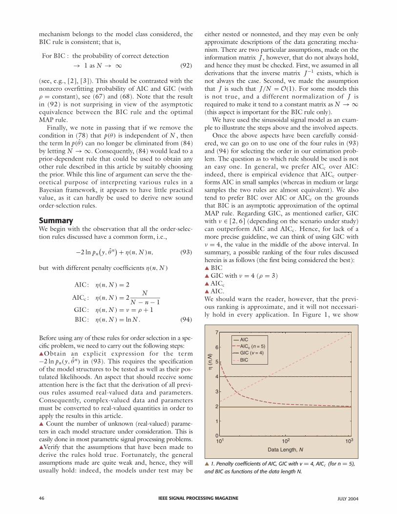
Once the above aspects have been carefully consid-ered, we can go on to use one of the four rules in (93)and (94) for selecting the order in our estimation prob-lem. The question as to which rule should be used is notan easy one. In general, we prefer AICc over AIC:indeed, there is empirical evidence that AICc outper-forms AIC in small samples (whereas in medium or largesamples the two rules are almost equivalent). We alsotend to prefer BIC over AIC or AICc on the groundsthat BIC is an asymptotic approximation of the optimalMAP rule. Regarding GIC, as mentioned earlier, GICwith ν ∈ [2, 6] (depending on the scenario under study)can outperform AIC and AICc. Hence, for lack of amore precise guideline, we can think of using GIC withν = 4, the value in the middle of the above interval. Insummary, a possible ranking of the four rules discussedherein is as follows (the first being considered the best):▲ BIC▲ GIC with ν = 4 (ρ = 3)▲ AICc▲ AIC.We should warn the reader, however, that the previ-ous ranking is approximate, and it will not necessari-ly hold in every application. In Figure 1, we show


▲ 1. Penalty coefficients of AIC, GIC with v = 4, AICc (for n = 5),and BIC as functions of the data length N.

AICAICc (n = 5)GIC (v = 4)

BIC

7

6

5

4

3

2

1

0

η (

n,N

)

101 102 103

Data Length, N

the penalty coefficients of the above rules, as func-tions of N , to further illustrate the relationshipbetween them.

Finally, we note that in the interest of brevity we willnot include numerical examples with the order-selec-tion rules under discussion but instead refer the readerto the abundant literature on the subject; see, e.g., [1]–[6], [30]–[32]. In particular, a forthcoming article[37] contains a host of numerical examples with theinformation criteria discussed in this review, along withgeneral guidelines as to how a numerical study of anorder-selection rule should be organized and what per-formance measures should be used.

AcknowledgmentsWe are grateful to Prof. Randolph Moses for his assis-tance in the initial stages of preparing this article. Thiswork was partly supported by the Swedish ScienceCouncil (VR). For more details on the topic of the arti-cle and its connections with other topics in signal pro-cessing, the reader may consult the book SpectralAnalysis of Signals by P. Stoica and R. Moses (Prentice-Hall, 2004).

Petre Stoica is a professor of system modeling atUppsala University in Sweden. For more details, seehttp://www.syscon.uu.se/Personnel/ps/ps.html.

Yngve Selén received the M.Sc. degree in engineeringphysics in 2002. He is currently a Ph.D. student ofelectrical engineering with specialization in signal pro-cessing at the Department of Information Technology, Uppsala University, Sweden.

References[1] B. Choi, ARMA Model Identification. New York: Springer-Verlag, 1992.

[2] T. Söderström and P. Stoica, System Identification. London, U.K.: Prentice-Hall Int., 1989.

[3] A.D.R. McQuarrie and C.-L. Tsai, Regression and Time Series ModelSelection. Singapore: World Scientific, 1998.

[4] H. Linhart and W. Zucchini, Model Selection. New York: Wiley, 1986.

[5] K.P. Burnham and D.R. Anderson, Model Selection and Multi-ModelInference. New York: Springer-Verlag, 2002.

[6] Y. Sakamoto, M. Ishiguro, and G. Kitagawa, Akaike Information CriterionStatistics. Tokyo, Japan: KTK Scientific, 1986.

[7] P. Stoica, P. Eykhoff, P. Janssen, and T. Söderström, “Model structureselection by cross-validation,” Int. J. Control, vol. 43, pp. 1841–1878,1986.

[8] T.W. Anderson, The Statistical Analysis of Time Series. New York: Wiley,1971.

[9] R.J. Brockwell and R.A. Davis, Time Series—Theory and Methods, 2nd ed.New York: Springer-Verlag, 1991.

[10] E.J. Hannan and M. Deistler, The Statistical Theory of Linear Systems. NewYork: Wiley, 1992.

[11] A. Papoulis, Signal Analysis. New York: McGraw-Hill, 1977.

[12] B. Porat, Digital Processing of Random Signals—Theory and Methods.Englewood Cliffs, NJ: Prentice-Hall, 1992.

[13] M.B. Priestley, Spectral Analysis and Time Series. London, U.K.:Academic, 1989.

[14] L.L. Scharf, Statistical Signal Processing—Detection, Estimation and TimeSeries Analysis. Reading, MA: Addison-Wesley, 1991.

[15] C.W. Therrien, Discrete Random Signals and Statistical Signal Processing.Englewood Cliffs, NJ: Prentice-Hall, 1992.

[16] L. Ljung, System Identification—Theory for the User, 2nd ed. UpperSaddle River, NJ: Prentice-Hall, 1999.

[17] B. Ottersten, M. Viberg, P. Stoica, and A. Nehorai, “Exact and large sam-ple ML techniques for parameter estimation and detection in array process-ing,” in Radar Array Processing, S. Haykin, J. Litva, and T.J. Shepherd,Eds. Berlin, Germany: Springer-Verlag, 1993, pp. 99–151.

[18] P. Stoica and A. Nehorai, “Performance study of conditional and uncon-ditional direction-of-arrival estimation,” IEEE Trans. Acoust., Speech,Signal Processing, vol. 38, pp. 1783–1795, Oct. 1990.

[19] H.L. Van Trees, Optimum Array Processing (Detection, Estimation, andModulation Theory, vol. 4). New York: Wiley, 2002.

[20] P. Stoica and R. Moses, Introduction to Spectral Analysis. Upper SaddleRiver, NJ: Prentice-Hall, 1997.

[21] P. Djuric’, “Asymptotic MAP criteria for model selection,” IEEE Trans.Signal Processing, vol. 46, pp. 2726–2735, 1998.

[22] H.L. Van Trees, Detection, Estimation, and Modulation Theory, Part I.New York: Wiley, 1968.

[23] S. Kullback and R.A. Leibler, “On information and sufficiency,” Ann.Math. Statist., vol. 22, pp. 79–86, Mar. 1951.

[24] H. Akaike, “A new look at statistical model identification,” IEEE Trans.Automat. Contr., vol. 19, pp. 716–723, Dec. 1974.

[25] H. Akaike, “On the likelihood of a time series model,” The Statistician,vol. 27, no. 3, pp. 217–235, 1978.

[26] R.L. Kashyap, “Inconsistency of the AIC rule for estimating the order ofAR models,” IEEE Trans. Automat. Contr., vol. 25, no. 5, pp. 996–998,Oct. 1980.

[27] R.J. Bhansali and D.Y. Downham, “Some properties of the order of anautoregressive model selected by a generalization of Akaike’s FPE criteri-on,” Biometrika, vol. 64, pp. 547–551, 1977.

[28] C. Hurvich and C. Tsai, “A corrected Akaike information criterion forvector autoregressive model selection,” J. Time Series Anal., vol. 14, pp. 271–279, 1993.

[29] J.E. Cavanaugh, “Unifying the derivations for the Akaike and correctedAkaike information criteria,” Statist. Probability Lett., vol. 33, pp. 201–208, Apr. 1977.

[30] S. de Wade and P.M.T. Broersen, “Order selection for vector autoregres-sive models,” IEEE Trans. Signal Processing, vol. 51, pp. 427–433, Feb. 2003.

[31] P.M.T. Broersen, “Finite sample criteria for autoregressive orderselection,” IEEE Trans. Signal Processing, vol. 48, pp. 3550–3558,Dec. 2000.

[32] P.M.T. Broersen, “Automatic spectral analysis with time series models,”IEEE Trans. Instrum. Meas., vol. 51, pp. 211–216, Apr. 2002.

[33] G. Schwarz, “Estimating the dimension of a model,” Ann. Statist., vol. 6,no. 2, pp. 461–464, 1978.

[34] R.L. Kashyap, “Optimal choice of AR and MA parts in autoregressivemoving average models,” IEEE Trans. Pattern Anal. Machine Intell., vol.4, no. 2, pp. 99–104, 1982.

[35] J. Rissanen, “Modeling by shortest data description,” Automatica, vol.14, no. 5, pp. 465–471, 1978.

[36] J. Rissanen, “Estimation of structure by minimum descriptionlength,” Circuits, Syst. Signal Process., vol. 1, no. 4, pp. 395–406,1982.

[37] P. Stoica and Y. Selén, “Multi-model approach to model selection,” IEEESignal Processing Mag., to be published.


model order selection - sal€¦ · model order selection as a hypothesis testing problem, with the...

Documents