model predictive control, the economy, and the issue of ... · model predictive control, the...
TRANSCRIPT

Ann Oper Res (2014) 220:25–48DOI 10.1007/s10479-011-0881-8
Model predictive control, the economy,and the issue of global warming
Thierry Bréchet · Carmen Camacho ·Vladimir M. Veliov
Published online: 7 April 2011© Springer Science+Business Media, LLC 2011
Abstract This study is motivated by the evidence of global warming, which is caused byhuman activity but affects the efficiency of the economy. We employ the integrated assess-ment Nordhaus DICE-2007 model (Nordhaus, A question of balance: economic modeling ofglobal warming, Yale University Press, New Haven, 2008). Generally speaking, the frame-work is that of dynamic optimization of the discounted inter-temporal utility of consump-tion, taking into account the economic and the environmental dynamics. The main noveltyis that several reasonable types of behavior (policy) of the economic agents, which may benon-optimal from the point of view of the global performance but are reasonable form anindividual point of view and exist in reality, are strictly defined and analyzed. These includethe concepts of “business as usual”, in which an economic agent ignores her impact on theclimate change (although adapting to it), and of “free riding with a perfect foresight”, wheresome economic agents optimize in an adaptive way their individual performance expectingthat the others would perform in a collectively optimal way. These policies are defined ina formal and unified way modifying ideas from the so-called “model predictive control”.
This research was supported by the Belgian Science Policy under the CLIMNEG project (SD/CP/05A).The second author was supported by the PAI grant P6/07 and from the Belgian French speakingcommunity Grant ARC 03/08-302. The third author was partly financed by the Austrian ScienceFoundation (FWF) under grant No P18161-N13.
T. Bréchet (�)CORE and Louvain School of Management, Chair Lhoist Berghmans in Environmental Economics andManagement, Université catholique de Louvain, Voie du Roman Pays, 34, 1348 Louvain-la-Neuve,Belgiume-mail: [email protected]
C. CamachoBelgian National Foundation of Scientific Research and Economics Department, Université catholiquede Louvain, Voie du Roman Pays, 34, 1348 Louvain-la-Neuve, Belgiume-mail: [email protected]
V.M. VeliovORCOS, Institute of Mathematical Methods in Economics, Vienna University of Technology,Argentinierstrasse 8, 1040 Vienna, Austriae-mail: [email protected]

26 Ann Oper Res (2014) 220:25–48
The introduced concepts are relevant to many other problems of dynamic optimization, es-pecially in the context of resource economics. However, the numerical analysis in this paperis devoted to the evolution of the world economy and the average temperature in the next150 years, depending on different scenarios for the behavior of the economic agents. In par-ticular, the results show that the “business as usual”, although adaptive to the change of theatmospheric temperature, may lead within 150 years to increase of temperature by 2°C morethan the collectively optimal policy.
Keywords Environmental economics · Dynamic optimization · Optimal control · Globalwarming · Model predictive control · Integrated assessment
1 Introduction
In his seminal paper, Nordhaus (1992) elaborated the very first integrated assessment model(IAM) of the world economy with global warming, the DICE model.1 This paper has beenfollowed by a plethora of quite similar computational models. Surprisingly, almost all ofthem are computed under only two basic runs: an optimal policy (the one that maximizesintertemporal welfare) and a business-as-usual scenario (no emission abatement). It is bycomparing these two scenarios that the benefits of a global climate policy are assessed. Thetypical message provided by IAMs is that slowing down the increase in greenhouse gasesis efficient, while stronger emission reductions would impose significant economic costs.Several modeling developments have been carried out to make IAMs more complex or morerealistic (backstop technologies, endogenous growth, resource exhaustion, etc.), but the twobasic scenarios remain. Our aim is to propose alternative—and arguably more realistic—ways to define business-as-usual scenarios in integrated assessment models. By doing this,we also question the costs and benefits of climate policies.
Let us start by explaining why we consider that the two basic scenarios used in IAMs(“optimal policy” and “business-as-usual”) may be subject of concerned. The reasons whythe “optimal policy” cannot be seen as realistic are well-established in the literature. Theoptimal policy scenario consists in maximizing the intertemporal welfare in the economy.It thus assumes a perfect foresight and benevolent policy makers, or a single representativeperfect foresight private agent, which is, in both cases, far from realism. For this reason,many authors consider that the optimal scenario just provides a Pareto efficient solution andis not to be considered as a policy scenario as such. As the best achievable solution, it isa benchmark, but it has little policy relevance. We follow this interpretation. As far as thebusiness-as-usual (hereafter, BaU) scenario is concerned, the drawbacks are of a differentnature. Nordhaus, as well as the following authors, define the BaU scenario as the trajectoryin productive investment that maximizes intertemporal welfare net of the damages incurredby global warming, but without emission abatement. In other words, the agent is still perfectforesighted, but she does not see the impacts of her own decisions on climate change andthe related damages she will bear. This scenario is not only unrealistic (because of perfectforesight), but it is also rationally inconsistent (because of a combination of perfect foresightand myopia about climate damages). This is the scenario we question in this paper.2
1The acronym DICE stands for “Dynamic Integrated Climate-Economy”. The first version of the DICE modelcan also be found in Nordhaus (1993) and Nordhaus (1993). See Nordhaus (2008) for the latest version. Themodel is publicly available on Nordhaus’ web page.2It is only when the model distinguishes many regions or countries that it becomes able to compute alternativescenarios based on coalitions of countries. The non-cooperative Nash equilibrium is the one where each

Ann Oper Res (2014) 220:25–48 27
Roughly speaking, we model the behavior of an agent doing BaU in the following way:the agent optimizes her economic objective disregarding her influence on the environmentand taking the state of the environment as exogenously given. If at some later time the agentencounters changed environmental conditions, then she updates her optimal policy regardingthe new environmental state, but still ignoring the impact of her economic activity on theenvironment. The same approach of the BaU is repeated persistently. We formalize this typeof behavior by introducing an idealized version of the BaU-agent which is independent ofthe time between subsequent updates. This is done in a general framework in which thebehavior of the economic agents is based on exogenous predictions for the evolution of theenvironment instead of predictions regarding the environmental impact of their economicpolicies. In particular, also a type of agent’s behavior that resembles the basic features offree riding (FR) is well defined in our framework as corresponding to a particular predictionpattern. Even more, we extend our general concept of prediction-based optimality to thecase of multiple agents who may implement different decision concepts: some regardingtheir impact on the environment, others doing business-as-usual or free riding. The sameframework seems to be relevant and may find interesting applications in other problems inresource economics.
The modeling technique that we employ in defining the above solution (behavioral)concepts adapts ideas from an area in the engendering-oriented control theory known asmodel predictive control or receding horizon control (see e.g. Allgöwer and Zheng 2000;Diehl et al. 2002; Findeisen et al. 2007). The above theory originates from problems ofstabilization of mechanical systems and its translation to the optimal control context in thepresent paper rises a number of mathematical problems that are not profoundly studied inthe literature. The key one is the issue of Lipschitz dependence of the optimal control ina long-horizon optimal control problem on the initial data and on the optimization horizon(we refer to Carlson et al. 1991; Dontchev and Rockafellar 2009 for a relevant information).In this paper we take a shortcut by formulating as assumptions all the properties neededfor the correct definition and results concerning the agent’s behavior. These assumptionslook at first glance cumbersome, but they are quite natural and essential. The verificationof some of the assumed properties is not easy, in general, and provides an agenda for a fu-ture research. In addition, the fulfillment of these assumptions in the main case study in thispaper—the global warming—is rather conditional, as one can learn from the rather strikingresults in Greiner and Semmler (2005) and Greiner et al. (2009), but still possible, as arguedin Appendix B.
Our problem is closely related to the literature in game theory literature in environmentaleconomics. In this stream, some authors have investigated the problem of agents interaction,their optimal actions and climatic consequences in more detailed IAMs. First, the WorldInduced Technological Change Hybrid (WITCH) model has produced richer results usinga game theoretical approach (see for an introduction Bosetti et al. 2009). In this model,12 world regions play an open-loop Nash game, choosing whether to cooperate on GHGemission control forming a coalition, and their decision depends on damages and abatementcosts. Haurie (2005) proposes an intergenerational game where each generation payoff de-pends on the welfare of all future generations. Haurie chooses a reduced version of theDICE94 model, as we do, although his climate block is more detailed. Each generation
country implements its optimal policy by taking the strategy of the other countries as given. Because of theglobal externality, it is inefficient. The full cooperative equilibrium is the one where all countries cooperate,and it coincides with the Pareto solution. In between, any coalition can be considered. For such analyses, seee.g. Bréchet et al. (2010), Bosetti et al. (2009), Eyckmans and Tulkens (2003), Yang (2008).

28 Ann Oper Res (2014) 220:25–48
has control over the economy during their lifetime and take their consumption/investmentdecisions for the period, taking into account the unknown decisions of the future genera-tions. In the numerical part of the paper it is shown that the optimal policy under altruismincreases environmental concern, achieving a higher capital accumulation and reduction inemissions via a more active abatement policy. One last example is the Climneg World Simu-lation Model (CWS), a 18-region model with flexible aggregation. In Eyckmans and Tulkens(2003) and Bréchet et al. (2011) the CWS model is used to scrutinize and compare the pol-icy implications that can be drawn from cooperative and non-cooperative game theoreticalframeworks.
The paper is organized as follows. Our modification of the Nordhaus integrated assess-ment model is presented in the next section. In Sect. 3 we introduce the general concept ofprediction-based optimality and the particular cases of BaU and FR. This concepts are ex-tended in Sect. 4 to the case of co-existing agents with different behavior. Then in Sect. 5 wepresent and discuss numerical results for the global warming problem. The two appendixesthat follow summarize some technical issues.
2 The world economy facing global warming
Our modeling of the world economy relies on the DICE-2007 model (see Nordhaus 2008).In a nutshell, there exists a policy maker who maximizes discounted welfare, integratingin the analysis the economic activity with its production factors, CO2 emissions and itsconsequences on climate change. Our climate block reduces to two equations which describethe dynamics of the concentration of CO2 (depending on emissions) and the interactionbetween CO2 concentration and temperature change. In this sense, our modeling looks likeprevious DICE versions in which the carbon-cycle was not detailed.3
The economy is populated by a constant number of individuals, which we normalizeto 1.4 A single final good is produced. This good can either be consumed, invested in thefinal good sector or used to abate CO2 emissions. A representative agent chooses optimalconsumption and abatement time-dependent policies aiming at maximization of the totalinter-temporal discounted utility from consumption (net of climate damages). The modelinvolves the physical capital, k(t), the CO2 concentration in the atmosphere, m(t), and theaverage temperature, τ(t), as state variables. The decision (control) variables are: u(t)—fraction of the GDP used for consumption, and a(t)—emission abatement rate. The overallmodel is formulated in the next lines and explained in detail below:
maxu,a
{∫ ∞
0e−rt [u(t)Y (t)]1−α
1 − αdt
}(1)
subject to (the argument t of k, τ and m is suppressed):
k = −δk + [1 − u(t) − c(a(t))]Y (t), k(0) = k0, (2)
τ = −λ(m)τ + d(m), τ (0) = τ 0, (3)
3The approach proposed in this paper applies to a rather general class of ODE models (see Sects. 3, 4) andcan be easily adapted to more elaborated IAMs than the one numerically analyzed in this paper.4Naturally, considering a changing population size over time would be more realistic and would change thenumerical results presented below, but it plays no role for the analytic concepts developed in the next twosections.

Ann Oper Res (2014) 220:25–48 29
m = −νm + (1 − a(t)) e(t)Y (t) + E(τ), m(0) = m0, (4)
Y (t) = p(t)ϕ(τ )kγ , u(t), a(t) ∈ [0,1]. (5)
The intertemporal elasticity of substitution of the utility in (1) with respect to consumptionis denoted by α ∈ (0,1), while r > 0 is the discount rate.
Production is realized through a Cobb-Douglas production function with elasticity γ ∈(0,1) with respect to physical capital. A fraction u of the output is consumed and anotherpart, c(a), is devoted to CO2 abatement. Here c(a) is the fraction of the output that is used forreducing the emission intensity by a fraction a.5 The function p(t) stands for productivitylevel and is assumed exogenous, while ϕ(τ) represents the impact of the climate on globalfactor productivity. Physical capital accumulation is described by (2) where the depreciationrate is δ > 0.
The evolution of CO2 concentration is depicted by (4), where ν is the natural absorp-tion rate, E(τ) is the non-industrial emission at temperature τ , and e(t) is the emissionfor producing one unit of final good without abatement. Finally, (3) establishes the linkbetween CO2 concentration and temperature change. The CO2 concentration increases theatmospheric temperature directly through d but also may affect the cooling rate λ. The initialvalues for the state variables k0, τ 0, m0 are given.
The numerical investigation of this model and its versions developed in the next two sec-tions is postponed to Sect. 5, where all the above data are specified. However, before turningto numerical analysis, we shall introduce in the next two sections two alternative solutionconcepts reflecting possible non-optimal, but still rational and realistic agent’s behavior.
3 Prediction-based optimality: a general consideration
In this section we consider a more general optimal control framework in which we presentthe basic concept introduced in this paper—that of prediction-based optimality—and someof its particular cases. In the explanations below we use the economic/environment inter-pretation of the variables given in the above section, although several different economicinterpretations are meaningful.
Consider the optimal control problem
maxv
∫ ∞
0L(t, v(t), x(t), y(t))dt (6)
subject to the dynamic constraints
x(t) = f (t, v(t), x(t), y(t)), (7)
y(t) = g(t, e(t, v(t), x(t)), y(t)), (8)
x(0) = x0, y(0) = y0, (9)
and the control constraint
v(t) ∈ V. (10)
5Notice that u + c(a) may be greater than one, in principle, in which case existing capital stock is sacrificedfor lower emission rate.

30 Ann Oper Res (2014) 220:25–48
The state variable x ∈ Rn is interpreted as a vector of stocks of economic factors, while thestate variable y ∈ Rm represents “environmental” (in general sense) factors whose evolutiondepends on the economic activity through the function e. The control vector-variable v ∈V ⊂ Rr may be interpreted as investment/abatement in different sectors and (6) maximizesthe aggregated output (or utility). The function e(t, v, x) has values in a finite dimensionalspace and represents the impact of the economic control, v, and the economic state, x, onthe dynamics of the environment.
The measurable functions v : [0,∞) �→ V will be called admissible controls. The model(7)–(8) will be considered as relevantly representing the evolution of the environmental-economic system. Thus for any given economic input v(t) we identify the correspondingsolution x(t), y(t) with the real economic-environmental state.
The particular case of the world economy facing global warming, presented in the pre-vious section, corresponds to the specifications x = k, y = (m, τ), v = (u, a), e(t, v, x) =(1 − a(t)) e(t)p(t)ϕ(τ )Kγ .6
Let (v, x, y) be a solution of problem (6)–(10) (this problem is called further OPT). Ourbasic argument is that, in real life, the motives for the decision-makers are to a large extendself-interest. They are also narrow-minded in the sense where they are unable to grasp thewhole picture. The last token means that the agent does not necessarily believe, or is notfully aware of (8). As a consequence, agent’s decisions need not result in resembling theoptimal path (v, x, y). The question is now of how to define alternative behavioral patterns?Below we define a concept of optimality which is not directly based on the model (8) of theenvironment, rather, on a prediction of the future environment obtained otherwise. Namely,we assume that at any time s the representative economic agent obtains a prediction forthe environmental variable y(t) on a (presumably large) horizon [s, s + θ ], depending onthe history of y on some interval [s − κ, s] and on the current economic state x(s). Thisprediction will be given by a mapping (predictor) Es : Cm(s − κ, s) × Rn �→ Cm(s,∞), thatis, Es(y|[s−κ,s], x(s))(t), is the prediction of y(t) for t ≥ s that results from a history y|[s−κ,s]of y and the current economic state x(s). In fact, only the values y(t) for t ∈ [s, s + θ ] willbe taken into account in the construction below.7
3.1 Step-wise definition
The starting idea is rather similar to that of the so-called model predictive control, or reced-ing horizon control (see e.g. Allgöwer and Zheng 2000; Diehl et al. 2002; Findeisen et al.2007). It is that, at time t = 0, the agent uses the prediction y(t) = E (y|[−κ,0], x0)(t) to solvethe problem (6), (7), (9), (10) on the time horizon [0, θ ] (that is, with bounds of integrationin (6) set to [0, θ ] instead of [0,∞)). Notice that this problem involves only the economiccomponent of the overall model, while the environment y(t) is taken as exogenous. The op-timal control v, although obtained on the horizon [0, θ ], is implemented on a “small” timeinterval [0, t1], after which the agent observes that the actual value of the environment, y(t1),has changed from the predicted one and repeats the same procedure with an updated pre-
6Note that there is an overloading of notations: the dimensions m and r in the general model have nothing todo with the concentration m and the discount r , etc. This could in no way lead to a confusion.7Further on we skip the subscript s in Es , since it will be clear from the arguments of E . Moreover, the twoparticular predictors we shall consider below are shift-invariant, thus the subscript s is, in fact, redundant.

Ann Oper Res (2014) 220:25–48 31
diction for y given by E (y|[t1−κ,t1], x(t1))(t).8 The formal definition of the respective agent’sbehavior is given below.
Assume that the past data y(t) for t ∈ [−κ,0] are known. Let at times ti = ih the agentreevaluates the past evolution of the environmental state y by measurements, where h > 0 isa positive time-step; presumably h � θ . We denote σ = (h, θ) and define a path (vσ , xσ , yσ )
recursively as follows.Set yσ = y(t) for t ∈ [−κ,0], xσ (0) = x0. Assume that (vσ , xσ , yσ ) is already defined
on [0, tk], k ≥ 0. Consider the problem
maxv(t)∈V
∫ tk+θ
tk
L(t, v(t), x(t), yk(t))dt (11)
x(t) = f (t, e(t, v(t), x(t)), yk(t)), x(tk) = xσ (tk), (12)
where yk(t) = E (yσ|[tk−κ,tk ], x
σ (tk))(t) for t ∈ [tk, tk + θ ]. Let vk+1 be an optimal control ofthis problem on [tk, tk + θ ]. We define vσ on [tk, tk+1] as equal to vk+1, and extend continu-ously (xσ , yσ ) as the respective solution of (7), (8) on [tk, tk+1].
This recurrent procedure defines (vθh, x
θh, yθ
h) on [0,∞).The idea is clear: the agent follows his optimal policy based on the prediction for the
environment at time s for a future period of length h, after which she realizes that the realenvironment has declined from the prediction and re-solves the optimization problem againwith an updated prediction. The definition below is a mathematical idealization in which there-evaluation period h tends to zero. This makes the resulting process independent of theparticular choice of step h.
Definition 1 Every limit point of any sequence (vσ , xσ , yσ ) (defined as above) in the spaceLloc
1 (0,∞) × C(0,∞) × C(0,∞) when σ = (h, θ) −→ (0,+∞) (if such exists) will becalled prediction-based optimal solution.9
Remark 1 We stress that neither the existence nor the uniqueness of a prediction-based opti-mal solution is granted. “Academic” counterexamples can easily be constructed. Even more,for a similar “global warming” model as the one presented in Sect. 2 a non-uniqueness ofthe optimal solution for initial data lying on a certain “critical” hyperplane in the state spacewas established in Greiner et al. (2009). For this model the existence and the uniqueness of aprediction-based optimal solution are questionable for “critical” initial data. Therefore, theconditions for existence and uniqueness stated below in this section for a particular predic-tion map E , although not necessary in general, are essential.
3.2 Two special prediction mappings
Two special cases of prediction-based optimality for two different predictors E are of specialinterest: a business-as-usual scenario and a free-rider scenario.
8Such a step-wise revision is consistent with the fact that, in climate science, a climate regime is defined byaveraging a 30-year time period. So a changing in a climate regime can be statistically demonstrated onlyafter several decades.9A sequence zσ converges to z in C(0,∞) if it converges uniformly on every compact interval [0, T ]. A se-
quence vσ converges to v in Lloc1 (0,∞) if
∫ T0 |vσ (t) − v(t)|dt converges to zero for every T > 0.

32 Ann Oper Res (2014) 220:25–48
3.2.1 Business as Usual (BaU)
If the environmental quality y is slowly changing compared with the economic factors x,then the representative agent may interpret the observed changes of y as unpredictable orexogenous fluctuations around an equilibrium, not substantially affected by the economicactivity. In other words, it reflects some natural exogenous fluctuations (for example, theeffect of solar activity on the global temperature on earth’s surface). As a result, the agentmay reasonably take a time-invariant value for the expected value of y:
E (y|[s−κ,s])(t) ≡ 1
κ
∫ s
s−κ
y(θ) dθ,
or merely take the current value at s as a prediction of the future: E (y|[s−κ,s])(t) = y(s),t ∈ [s, s + θ ] (this corresponds to κ = 0).
This approach of the agents, which disregards the dynamics of the environment althoughadapting to its changes a posteriori, will be called Business as Usual (BaU).
The simplest case of BaU is that with κ = 0, which is realistic in a slowly changingenvironment. We shall formulate this particular case more explicitly. Consider the problem
maxv(t)∈V
∫ s+θ
s
L(t, x(t), y, v(t)) dt
x(t) = f (t, e(t, v(t), x(t)), y), x(s) = xs, t ∈ [s, s + θ ],where s ≥ 0, θ ∈ (0,∞), xs ∈ Rn and y ∈ Rm are given. Denote by v[s, θ, xs;y](t) asolution of this problem (assuming that such exists). Then the step-wise approximation(vσ , xσ , yσ ) of BaU for σ = (h, θ) can be written (recursively in k) as
vσ (t) = v[tk, θ, xσ (tk);yσ (tk)](t), t ∈ [tk, tk+1], (13)
(xσ , yσ ) solves (7), (8) with v = vσ . (14)
The initial conditions in (14) are given by (9) at tk = t0 = 0, while xσ , yσ are extended bycontinuity at each tk > 0.
Clearly, in the context of the previous section the BaU approach has been practically theonly one implemented by agents at all levels till the late 20th century, and is still dominatingin many countries. It consists in being conservative in the understanding of nature’s law.This BaU scenario, however, is rationally consistent.
3.2.2 Free riders (FR)
There exists a presumably large number of (identical or not) agents in the economy, whichtherefore can be viewed as represented (aggregated) by a single representative agent. Therepresentative agent determines the collectively optimal policy v by solving the problem(6)–(10). In particular, the y-component of the solution, y, gives the future developmentof the environment if the optimal policy were implemented by all agents. But some agentsmay free ride. A free rider is an agent that assumes that the other agents would implementthe optimal policy, and since the influence of a single agent on the environment is negligi-ble, she may take y(t) as predictor for the future environment and design her own optimalpolicy solving (6), (7), (9), (10) with y = y (which policy is, in general, different from thecollectively optimal one, v).

Ann Oper Res (2014) 220:25–48 33
In this section we consider an “extreme” scenario in which all agents undertake freeriding. In Sects. 4 and 5.3 we shall investigate the more realistic case of co-existing agentswith different behavior, some following the optimal policy regarding the influence of theeconomy on the environment (OPT), some others practicing BaU or FR.
Formally, the predictor E of a FR is defined as follows. Denote by (x[s, xs, ys],y[s, xs, ys]) the optimal trajectory of problem (6)–(10) on the interval [s,∞) (instead of[0,∞)) and with initial data x(s) = xs , y(s) = ys at time s (replacing (9)). Then the predic-tor E is defined as
E (y|[s−κ,s], x)(t) = y[s, x, y(s)](t).That is, the hypothetical collectively optimal evolution of the environment starting from thecurrent data is used as a predictor.
3.3 Feedback definition of BaU-solution: existence and uniqueness
Here we present another point of view to the optimality concepts introduced above focusingfor more transparency on the simplest BaU—that with κ = 0. The general case requiresappropriate modifications and assumptions concerning the predictor E .
Although in the assumptions below we do not seek generality (they are just reasonablygeneral, so that several applications satisfy them) they are rather implicit and will be dis-cussed in Appendix B. Assume the following:
Assumption A.1 (i) Let X ⊂ Rn, Y ⊂ Rm and V ∈ Rr be given sets and let E be a set con-taining all vectors e(t, v, x) with t ≥ 0, v ∈ V , x ∈ X. The functions f (t, v, x, y), g(t, e, y),L(t, v, x, y), e(t, v, x) are bounded, continuous in t and Lipschitz continuous in the rest ofthe variables, v ∈ V , x ∈ X, y ∈ Y and e ∈ E, uniformly with respect to t . Moreover, x0 ∈ X
and y0 ∈ Y .(ii) For every admissible control v, every s ≥ 0, xs ∈ X and ys ∈ Y the solution of (17),
(18), with initial conditions x(s) = xs , y(s) = ys , exists in X × Y on [s,∞).
Assumption A.2 (i) For every s ≥ 0, θ ∈ (0,∞), xs ∈ X and ys ∈ Y the optimal controlv[s, θ, xs;ys](·) exists and is unique in the space L1([s, s + θ ]).
(ii) There exist a number l and a continuous function δ : [0,∞) �→ [0,∞), with δ(0) = 0,such that for every t ≥ s ≥ 0, θ ≥ θ ≥ t − s, x, x ∈ X, y, y ∈ Y the following inequalityholds:
|v[s, θ, x;y](t) − v[t, θ , x; y](t)| ≤ l(|x − x| + |y − y|) + δ
(|s − t | + 1
θ
).
Let T be any positive number. Assumption A.2 together with the completeness ofthe space C([s, T ]) imply that for every s ∈ [0, T ], xs ∈ X and ys ∈ Y the sequencev[s, θ, xs;ys] converges in the space C([s, T ]) whit θ −→ ∞ to a continuous admissiblecontrol denoted by v[s,∞, xs;ys].
Proposition 1 Under Assumptions A.1, A.2 a unique BaU-solution in the sense of Defini-tion 1 exists and coincides with the unique solution of the feedback system
x(t) = f (t, v[t,∞, x(t);y(t)](t), x(t), y(t)), x(0) = x0, (15)
y(t) = g(t, e(t, v[t,∞, x(t);y(t)](t), x(t)), y(t)), y(0) = y0. (16)

34 Ann Oper Res (2014) 220:25–48
We skip the proof (which is a standard exercise in calculus), but in fact it is contained inthe proof of the more complicated Proposition 2, which is given in Appendix A.
The feedback system (15), (16) provides an alternative to Definition 1. This is an easyshortcut to the concept of BaU-solution. However, Definition 1 reflects in a better way thepractical BaU-behavior, where the stepwise policy vθ
h is implemented. Therefore the issueof convergence of the step-wise BaU-control vθ
h is of key importance for the credibility ofthe idealization (15), (16) and, in addition, provides a numerical approach for finding theBaU-solution, implemented in our numerical analysis of the global warming problem inSect. 5.
4 Co-existing agents with different behavior
In the previous section we considered the scenario in which all economic agents behavein the same way, therefore can be represented by a single agent which either optimizes bysolving the full economic-environment problem (6)–(10) (we call such an agent OPT), orchooses the BaU or the FR behavior. In the present section we consider the case of co-existence of agents with different behavior. For reasons of transparency we focus on thesimplest case of two agents (groups of countries): one OPT and one BaU.
Let v1 and v2 be the controls of the OPT and of the BaU, and x1 and x2 be their eco-nomic states. Assuming additivity of the environmental impact e of the economic activitiesof the two agents (which is the case if polluting emissions such as CO2 are considered), wereformulate the dynamics of the economic-environment system as
xi (t) = fi(t, vi(t), xi(t), y(t)), xi(0) = x0i , i = 1,2, (17)
y(t) = g(t, e1(t, v1(t), x1(t)) + e2(t, v2(t), x2(t)), y(t)), y(0) = y0, (18)
with the control constraints
vi(t) ∈ V, i = 1,2. (19)
The objective function of the agent i is
∫ ∞
0Li(vi(t), xi(t), y(t))dt. (20)
Here the finite dimensional vector ei(t, vi, xi) represents the instantaneous emission of theagent i resulting from control value vi and economic state xi at time t . Below we investigatethe evolution of such an economic-environment system, adapting the concept of BaU devel-oped in the previous section. Agent 2 optimizes her utility in a BaU manner, while agent 1optimizes her utility regarding the environmental change. The complication of the coexist-ing BaU and OPT agents comes from the fact that they live in a common environment, y(t),which they both influence, therefore their respective optimal policies are not independent ofeach other. Namely, in order to solve her problem OPT has to know the influence of BaU onthe environment. On the other hand, BaU adapts her decision to the environmental change(in a similar manner as in the previous section), which on its turn depends on the policy ofOPT.
The idea of the formal definition of co-existing OPT and BaU is as follows. The agentBaU (agent i = 2) first solves her optimal control problem (17), (19), (20) (with i = 2)on [0, θ ] using the predictor y(t) = y0. This defines a hypothetical emission η2(t) =
Ann Oper Res (2014) 220:25–48 35
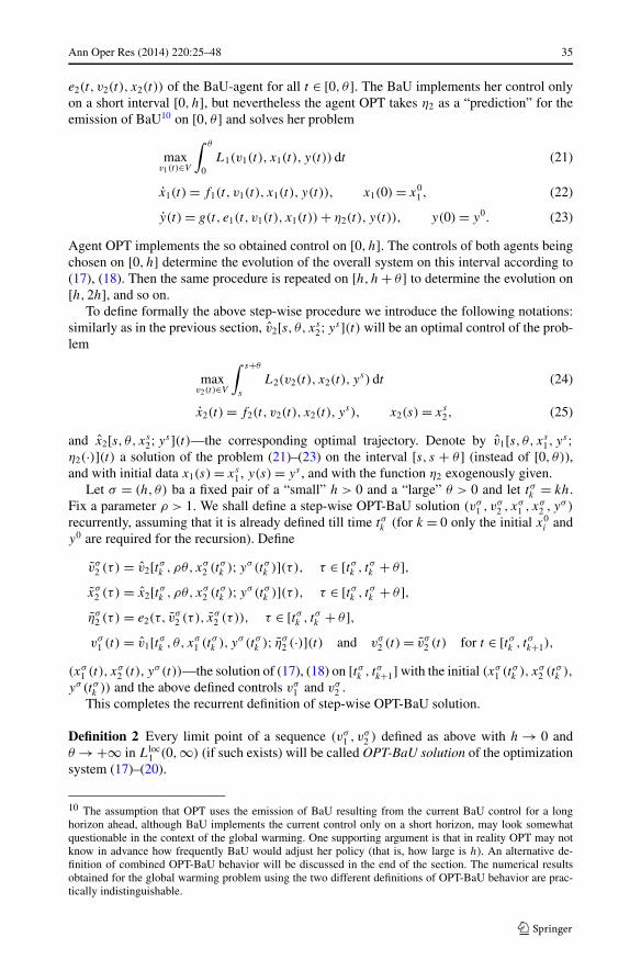
e2(t, v2(t), x2(t)) of the BaU-agent for all t ∈ [0, θ ]. The BaU implements her control onlyon a short interval [0, h], but nevertheless the agent OPT takes η2 as a “prediction” for theemission of BaU10 on [0, θ ] and solves her problem
maxv1(t)∈V
∫ θ
0L1(v1(t), x1(t), y(t)) dt (21)
x1(t) = f1(t, v1(t), x1(t), y(t)), x1(0) = x01 , (22)
y(t) = g(t, e1(t, v1(t), x1(t)) + η2(t), y(t)), y(0) = y0. (23)
Agent OPT implements the so obtained control on [0, h]. The controls of both agents beingchosen on [0, h] determine the evolution of the overall system on this interval according to(17), (18). Then the same procedure is repeated on [h,h + θ ] to determine the evolution on[h,2h], and so on.
To define formally the above step-wise procedure we introduce the following notations:similarly as in the previous section, v2[s, θ, xs
2;ys](t) will be an optimal control of the prob-lem
maxv2(t)∈V
∫ s+θ
s
L2(v2(t), x2(t), ys) dt (24)
x2(t) = f2(t, v2(t), x2(t), ys), x2(s) = xs
2, (25)
and x2[s, θ, xs2;ys](t)—the corresponding optimal trajectory. Denote by v1[s, θ, xs
1, ys;
η2(·)](t) a solution of the problem (21)–(23) on the interval [s, s + θ ] (instead of [0, θ)),and with initial data x1(s) = xs
1, y(s) = ys , and with the function η2 exogenously given.Let σ = (h, θ) ba a fixed pair of a “small” h > 0 and a “large” θ > 0 and let tσk = kh.
Fix a parameter ρ > 1. We shall define a step-wise OPT-BaU solution (vσ1 , vσ
2 , xσ1 , xσ
2 , yσ )
recurrently, assuming that it is already defined till time tσk (for k = 0 only the initial x0i and
y0 are required for the recursion). Define
vσ2 (τ ) = v2[tσk , ρθ, xσ
2 (tσk );yσ (tσk )](τ ), τ ∈ [tσk , tσk + θ ],xσ
2 (τ ) = x2[tσk , ρθ, xσ2 (tσk );yσ (tσk )](τ ), τ ∈ [tσk , tσk + θ ],
ησ2 (τ ) = e2(τ, v
σ2 (τ ), xσ
2 (τ )), τ ∈ [tσk , tσk + θ ],vσ
1 (t) = v1[tσk , θ, xσ1 (tσk ), yσ (tσk ); ησ
2 (·)](t) and vσ2 (t) = vσ
2 (t) for t ∈ [tσk , tσk+1),
(xσ1 (t), xσ
2 (t), yσ (t))—the solution of (17), (18) on [tσk , tσk+1] with the initial (xσ1 (tσk ), xσ
2 (tσk ),
yσ (tσk )) and the above defined controls vσ1 and vσ
2 .This completes the recurrent definition of step-wise OPT-BaU solution.
Definition 2 Every limit point of a sequence (vσ1 , vσ
2 ) defined as above with h → 0 andθ → +∞ in Lloc
1 (0,∞) (if such exists) will be called OPT-BaU solution of the optimizationsystem (17)–(20).
10 The assumption that OPT uses the emission of BaU resulting from the current BaU control for a longhorizon ahead, although BaU implements the current control only on a short horizon, may look somewhatquestionable in the context of the global warming. One supporting argument is that in reality OPT may notknow in advance how frequently BaU would adjust her policy (that is, how large is h). An alternative de-finition of combined OPT-BaU behavior will be discussed in the end of the section. The numerical resultsobtained for the global warming problem using the two different definitions of OPT-BaU behavior are prac-tically indistinguishable.

36 Ann Oper Res (2014) 220:25–48
Below we formulate conditions for existence of an OPT-BaU solution. Moreover, it willbe proved that the OPT-BaU solution is independent of the choice of the parameter ρ > 1 inthe step-wise definition.
Assumption A.1′ (i) Let X ⊂ Rn, Y ⊂ Rm and V ∈ Rr be given open sets and let E be a setcontaining all vectors e1(t, v1, x1) + e2(t, v2, x2) with t ≥ 0, vi ∈ V , xi ∈ X. The functionsfi(t, v, x, y), g(t, e, y), Li(t, v, x, y), ei(t, v, x) are bounded, continuous in t and Lipschitzcontinuous in the rest of the variables, v ∈ V , x ∈ X, y ∈ Y and e ∈ E, uniformly withrespect to t . Moreover, x0
i ∈ X and y0 ∈ Y .(ii) For every admissible controls v1 and v2, every s ≥ 0, xs
i ∈ X and ys ∈ Y the solutionof (17), (18), with initial conditions xi(s) = xs
i , y(s) = ys , exists in X × X × Y on [s,∞).
Assumption A.2′ (i) For every s ≥ 0, θ ∈ (0,∞), xs ∈ X, ys ∈ Y , and continuous η2 :[s, s + θ ] → E the optimal controls v1[s, θ, xs, ys;η2(·)](·) and v2[s, θ, xs;ys](·) exist andare unique in L1(s, s + θ).
(ii) There exist a number l, and continuous functions δ,α : [0,∞) �→ [0,∞), withδ(0) = 0, such that for every t ≥ s ≥ 0, θ ≥ θ ≥ t − s, x, x ∈ X, y, y ∈ Y and continuousfunctions continuous η2, η2 : [0,∞) �→ E the following inequality holds:
|v1[s, θ, x, y;η2](t) − v1[t, θ , x, y; η2](t)|
≤ l(|x − x| + |y − y|) + δ
(|t − s| + 1
θ
)+
∫ s+θ
t
α(τ − s)|η2(τ ) − η2(τ )|dτ.
(iii) There exist continuous functions δ,β : [0,∞) �→ [0,∞], with δ(0) = 0 and∫ ∞0 α(τ)β(τ)dτ < ∞, such that for every t ≥ s ≥ 0, θ ≥ θ ≥ 0, τ ∈ [t, s + θ), x, x ∈ X
and y, y ∈ Y the following inequality holds:
|v2[s, θ, x;y](τ ) − v2[t, θ , x; y](τ )| + |x2[s, θ, x;y](τ ) − x2[t, θ , x; y](τ )|
≤ β(τ − s)
(|x − x| + |y − y| + δ
(|s − t | + 1
s + θ − τ
)).
As mentioned in the Introduction, Assumption A.2′ looks very cumbersome, althoughthey just relevantly represent the requirement of Lipschitz dependence of the optimal solu-tion on the initial data and on the length of the horizon. What “relevantly” does mean here?For example, the nastier looking term δ in Assumption A.2′(iii) reflects the fact that the op-timal control on a long horizon [s, s + θ ] is strongly influenced near the end of the horizonby the fact that the optimization disregards what happens after s + θ . Thus the solution on[s, s + θ ] needs not be close to the one for a longer horizon θ for t near s + θ . The nextlemma claims that the dependence of the optimal solution on the length of the horizon issignificant only near the end of the horizon, that is, it melts out if the horizon is infinite.
Lemma 1 For every s ≥ 0, (x, y) ∈ X × Y and continuous η2 : [0,∞) �→ E the limits
v1[s,∞, x, y;η2](s) := limθ→∞ v1[s, θ, x, y;η2](s),
v2[s,∞, x;y](·) := limθ→∞ v2[s, θ, x;y](·), x2[s,∞, x;y](·) := lim
θ→∞ x2[s, θ, x;y](·)
exist, the last two in C(s,∞).

Ann Oper Res (2014) 220:25–48 37
The first claim follows from Assumption A.2′(ii) applied for t = s, x = x, y = y, η2 = η2.The second and the third ones use similarly Assumption A.2′(iii) and also the completenessof the space C(0, T ).
To shorten the notations we abbreviate
η2[x2, y](t, ·) = e2(·, v2[t,∞, x2;y](·), x2[t,∞, x2;y](·)),v1[x1, x2, y](t) = v1[t,∞, x1, y;η2[x2, y](t, ·)](t), v2[x2, y](t) = v2[t,∞, x2;y](t),η1[x1, x2, y](t) = e1(t, v1[x1, x2, y](t), x1).
Proposition 2 Under Assumptions A.1′ and A.2′, a combined OPT/BaU-optimal solutionin the sense of Definition 2 exists and coincides with the unique solution of the feedbacksystem
x1 = f (t, v1[x1, x2, y](t), x1, y), x1(0) = x01 , (26)
x2 = f (t, v2[x2, y](t), x2, y), x2(0) = x02 , (27)
y(t) = g(t, η1[x1, x2, y](t) + η2[x2, y](t, t), y), y(0) = y0, (28)
where the argument t of x1(t), x2(t) and y(t) is suppressed.
Notice that η2[x2, y](t, t) in (28) equals just e2(t, v2[t,∞, x2;y](t), x2).The proof is given in Appendix A.Similarly as for the case of a pure BaU solution, the approximate calculation of OPT-BaU
solutions makes use of the intuitive step-wise definition.As we mentioned in footnote 10 a different reasonable definition of OPT-BaU solution
may be given, which assumes more sophisticated behavior of the OPT-agent. Namely, inthe above step-wise definition OPT uses at every step the prediction of the future emissionη2(t) of BaU, not taking into account that BaU may adapt in the next time-period to thechange of the environmental variable y. A more involved OPT-agent may take into accountthe influence of her own decisions to the adjustment of the BaU-control.
Below we briefly formulate the resulting refined concept of OPT-BaU solution, consider-ing directly the “idealized” limit-version with infinite horizon and instantaneous adjustmentof BaU.
The definition will be of fixed-point type. Imagine that OPT bases her solution on a guessη2 ∈ Lloc
1 (0, T ) for the future emission of BaU. That is, OPT solves the problem
maxv1(t)∈V
∫ ∞
0L1(v1(t), x1(t), y(t)) dt
subject to
x1(t) = f1(t, v1(t), x1(t), y(t)), x1(0) = x01 ,
y(t) = g(t, e1(t, v1(t), x1(t)) + η2(t), y(t)), y(0) = y0.
Denote by (v∗1 [η2], x∗
1 [η2]) the economic component of the solution, and by η∗1[η2](t) =
e1(t, v∗1 [η2](t), x∗
1 [η2](t))—the corresponding emission. Then BaU obtains the BaU-optimalsolution (in the sense of Definition 1) of her problem (with the emission of OPT exogenouslygiven by η∗
1[η2](t)):
maxv2(t)∈V
∫ ∞
0L2(t, v2(t), x2(t), y(t)) dt

38 Ann Oper Res (2014) 220:25–48
subject to
x2(t) = f2(t, v2(t), x2(t), y(t)), x2(0) = x02 ,
y(t) = g(t, η1[η2](t) + e2(t, v2(t), x2(t)), y(t)), y(0) = y0.
Let (v∗2 [η2], x∗
2 [η2]) be BaU-optimal solution, thus η∗2[η2](t) = e2(t, v
∗2 [η2](t), x∗
2 [η2](t)) isthe resulting emission of the BaU-agent. Now we complete the definition by requiring thatthe initial guess of OPT is consistent with the obtained real emission output:
η∗2[η2] = η2. (29)
This is a functional equation that determines the “right” initial guess η2 of OPT.We do not address the apparently complicated issue of existence of a solution to the
above functional equation, since Definition 2 seems to be more relevant to the real behaviorof the OPT and BaU agents. In addition, iterating the fix-point equation (29), using as aninitial guess the BaU emission η2(t) in the OPT-BaU solution in sense of Definition 2 forour global warming model, we establish that there is no considerable difference between thetwo OPT-BaU solution concepts for this particular model. Therefore, further we focus onthe OPT-BaU solution concept given by Definition 2.
5 Numerical analysis of the world economy under global warming
In this section we provide numerical illustrations for the different decision patterns definedabove, with an application to the global warming issue. First, the computational model andits calibration are presented. Then we compute Business-as-Usual (BaU) and Optimal (OPT)scenarios and, in the last subsection, we consider the case of co-existing agents.
The calculations are performed in the following way. For a single OPT-agent one has tosolve the full-order optimal control problem (6)–(10) with the specifications in (1)–(5). Thisis done by cutting the time-horizon [0,∞) to [0, θ), where θ is so large that the solutionrestricted to the horizon [0,180] is practically independent of θ . Any θ > 250 turns outto be appropriate. On the finite horizon [0, θ ] the problem (6)–(10) is solved by a generalsolver of optimal control problems developed by the third author, which implements a gra-dient projection method in the control space, where the gradient of the objective function iscalculated by using the adjoint equation arising in the Pontryagin maximum principle. Thecalculations on a PC take a few seconds.
The procedure is more complicated for the single BaU solution, since at any time-steptk in the step-wise definition of BaU one has to solve the reduced-order problem (11), (12).This, however, is not problematic, since at every consequent interval [tk; tk + θ ] one can useas an initial guess for the control the one obtained for the interval [tk−1, tk−1 + θ ]. Only afew gradient iterations of the general solver are enough.
In the case of co-existing agents the numerical complexity doubles since also the OPT-agent has to resolve her problem at every time-step for the updated control policy of theBaU-agent. On a standard PC the calculation takes a few minutes.
5.1 The computational model and its calibration
The model is a DICE-type integrated assessment model of the climate and the economy. Thecalibration is made in such a way that we replicate the central scenarios in the Fourth As-

Ann Oper Res (2014) 220:25–48 39
Table 1 Parameters valueEconomic parameters
Depreciation rate δ 0.1
Intertemporal elasticity of substitution α 0.5
Interest rate r 0.005
Capital elasticity γ 0.75
Climate parameters
Temperature reabsorption λ 0.11
Climate sensitivity η 0.0054
Preindustrial carbon concentration m∗0 596.4
Damage function parameter θ1 0.0057
Damage function parameter θ2 2
CO2 reabsorption rate ν 0.0054
sessment Report IPCC in terms of carbon emissions and temperature increase.11 Therefore,there is nothing new in the modeling itself, since we want to focus on new behavioral rules.We compute numerically the economy described in Sect. 2 over a period of T = 300 years.To get rid of boundary effects we display results only for the first 175 years. The time sliceis the year, and for the discretization scheme we choose a time step h = 0.05 years. Table 1displays the parameters value and initial conditions for the economic and climatic parts ofthe model. We have deliberately chosen a low value for the interest rate (with respect to thevalues chosen by Nordhaus in the DICE model) because of the arguments given by Hau-rie (2003) and Stern (2006). We consider that, given the length of our exercise, such a lowvalue is necessary to fully take into account the welfare of far future generations. The initialvalues for the state variables are k0 = 733.2, the initial value of physical capital (in billiondollars), m0 = 808.9, the carbon concentration in 2005 (in GtC) and τ0 = 0.7307 the initialtemperature increase (between 1900 and 2005, in °C).
In what follows, we describe the functional forms for the functions p, e, ϕ, c and d . Thereexists an exogenous technological progress, p(t). It is a linear function of time such thatp(0) = 1 and p(175) = 1.25. The exogenous technology which reduces carbon emissionintensity with time, e(t), is an exponential function verifying that e(0) = 0.0427 and e(75) =0.75e(0); i.e. we assume an exogenous decrease in the emission output intensity by 25% in75 years. All these assumptions are within common ranges.12
The damage function has a standard formulation ϕ(τ) = 1/(1 + θ1τθ2). The calibration
captures the impact of global warming on global productivity: a 2°C increase in the meantemperature reduces the global productivity by 3%. We assume c(a) = 0.01a/(1 − a); i.e.c(0) = 0 and lima→1 c(a) = ∞. The calibration implies that reducing the emission outputintensity by 50% incurs a cost of 1% of GDP. The effect of CO2 concentration on the averagetemperature increase is captured by the standard function d(m) = η ln(m/m∗
0): a doublingof CO2 concentration increases the average temperature by 0.41°C, where m∗
0 = 596.4 GtCis the preindustrial CO2 concentration in the atmosphere.
11The calibration is done so that the BaU scenario yields a temperature increase of 3°C in 2050 over the1900 level. This increase lies within the confidence interval for the non-mitigation emission scenarios A1B,A1F1, A1T in Chap. 10 of the Contribution of Working Group I to the Fourth Assessment Report of theIntergovernmental Panel on Climate Change (see Solomon et al. 2007). This report is available on line at:www.ipcc.ch.12See Solomon et al. (2007), Nordhaus (2008), Stern (2006) and Yang (2008).

40 Ann Oper Res (2014) 220:25–48
Fig. 1 BaU convergence. Shareof output consumed. Legend:BaU 10 years (dashes), BaU 5years (dots)
Anticipating our results, we obtain that when the economy consists only on OPT agents,the temperature increase after 175 years is roughly 3°C with respect to the 2005 level. Ifthere are only BAU agents, temperature increases almost 5°C for the same period. This 2°Cdifference is crucial. Indeed, Stern (2006) estimates a 5–20% loss of gross world productwith probability 0.1 if temperature increases more than 5°C. Nordhaus and Boyer (2000)foresees a 25% loss with probability 0.012 for an increase of 2.5°C. If the increase was of6°C the probability would be five times larger. Kriegler et al. (2009) have estimated that foran increase of 2–4°C over the temperature in 2000 could trigger a major change in the earthsystem with probability 0.16 and with probability 0.56 if the temperature change is above4°C.
5.2 A comparison between BaU and OPT scenarios
The first exercise we perform shows convergence of the BaU trajectory as revisions takeplace more frequently. Figure 1 shows the trajectory for the share of output to be consumed,u, under two BaU scenarios in which two revision schemes are considered, after 10 years(dashed line) and after 5 years (dotted line). One can see that the trajectory converges to-wards a smooth BaU as the revision scheme becomes shorter. When the revision schemeis slow, (every 10 years) the share of output that is consumed moves too slowly. In otherwords, too much capital is invested in order to have more consumption in the future. Thetrade-off between consumption and investment is biased because the agent under-estimatesthe climate damages that will occur in the far future. When the revision occurs, the agentrealizes her mistake and she sharply decreases capital accumulation. But then again, shemakes the same kind of mistake during a decade. This balance between the mistake (toomuch capital accumulation and too much emissions) and the revision becomes smootheras the economy approaches the steady state. It must be noticed that the correction is sharpbecause there are no adjustment costs in our model. The movements in consumption wouldbe smoother if adjustment costs were considered on capital accumulation or on emissionabatement.
Next we have computed the world economy in which the OPT policy maker can abate,i.e. she can devote a share of output to reduce CO2 emissions. Results for the OPT and BaUscenarios are displayed in Fig. 2.

Ann Oper Res (2014) 220:25–48 41
Fig. 2 Optimal solutions under abatement. Legend: OPT (solid line), BaU (dotted line)
In the OPT scenario, the share of output that is consumed (panel a) is always largerthan in the BaU scenario. It results that capital accumulation is always smaller (panel d).Interestingly, the gap between these two trajectories shrinks with time (panels d), and thecapital stock is almost the same in the two scenarios at the end of the simulation period.Hence, what makes the difference between the two scenarios is the transition path.
Actually, the consumption level is not always higher in OPT than in BaU (despite the factthat the share is always higher). Let us study the reasons: BaU’s larger investment inducesnot only a larger level of physical capital and production in the future (all else equal) butalso more emissions and consequently a larger temperature increase. Damages only comeout in the long run. So at the beginning of the simulation period, consumption level is higheris OPT, but because the BaU accumulates more capital, it brings a larger consumption levelbetween period 35 and 88. After period 85, the costs of global warming become large andcapital accumulation is refrained in BaU while consumption is again larger in OPT. Thefeed-back effect of climate on the economy is sharp: economic growth is almost zero inBaU after period 60.
Panel (b) shows the abatement rate. Provided the abatement cost function we have cho-sen, an abatement rate of 45% is optimal since the very first time period. Abatement thenincreases and reaches its maximum after 40 years at roughly 52%. In the long run, emissionsare thus cut by 33%. As a result, under this OPT scenario the temperature is reduced in thelong-run by 2°C with respect to the BaU scenario.
42 Ann Oper Res (2014) 220:25–48
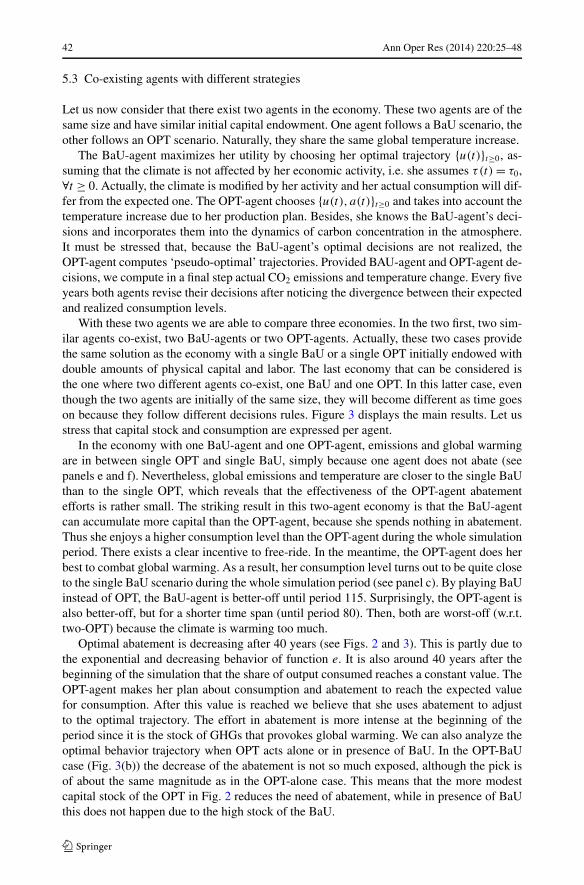
5.3 Co-existing agents with different strategies
Let us now consider that there exist two agents in the economy. These two agents are of thesame size and have similar initial capital endowment. One agent follows a BaU scenario, theother follows an OPT scenario. Naturally, they share the same global temperature increase.
The BaU-agent maximizes her utility by choosing her optimal trajectory {u(t)}t≥0, as-suming that the climate is not affected by her economic activity, i.e. she assumes τ(t) = τ0,∀t ≥ 0. Actually, the climate is modified by her activity and her actual consumption will dif-fer from the expected one. The OPT-agent chooses {u(t), a(t)}t≥0 and takes into account thetemperature increase due to her production plan. Besides, she knows the BaU-agent’s deci-sions and incorporates them into the dynamics of carbon concentration in the atmosphere.It must be stressed that, because the BaU-agent’s optimal decisions are not realized, theOPT-agent computes ‘pseudo-optimal’ trajectories. Provided BAU-agent and OPT-agent de-cisions, we compute in a final step actual CO2 emissions and temperature change. Every fiveyears both agents revise their decisions after noticing the divergence between their expectedand realized consumption levels.
With these two agents we are able to compare three economies. In the two first, two sim-ilar agents co-exist, two BaU-agents or two OPT-agents. Actually, these two cases providethe same solution as the economy with a single BaU or a single OPT initially endowed withdouble amounts of physical capital and labor. The last economy that can be considered isthe one where two different agents co-exist, one BaU and one OPT. In this latter case, eventhough the two agents are initially of the same size, they will become different as time goeson because they follow different decisions rules. Figure 3 displays the main results. Let usstress that capital stock and consumption are expressed per agent.
In the economy with one BaU-agent and one OPT-agent, emissions and global warmingare in between single OPT and single BaU, simply because one agent does not abate (seepanels e and f). Nevertheless, global emissions and temperature are closer to the single BaUthan to the single OPT, which reveals that the effectiveness of the OPT-agent abatementefforts is rather small. The striking result in this two-agent economy is that the BaU-agentcan accumulate more capital than the OPT-agent, because she spends nothing in abatement.Thus she enjoys a higher consumption level than the OPT-agent during the whole simulationperiod. There exists a clear incentive to free-ride. In the meantime, the OPT-agent does herbest to combat global warming. As a result, her consumption level turns out to be quite closeto the single BaU scenario during the whole simulation period (see panel c). By playing BaUinstead of OPT, the BaU-agent is better-off until period 115. Surprisingly, the OPT-agent isalso better-off, but for a shorter time span (until period 80). Then, both are worst-off (w.r.t.two-OPT) because the climate is warming too much.
Optimal abatement is decreasing after 40 years (see Figs. 2 and 3). This is partly due tothe exponential and decreasing behavior of function e. It is also around 40 years after thebeginning of the simulation that the share of output consumed reaches a constant value. TheOPT-agent makes her plan about consumption and abatement to reach the expected valuefor consumption. After this value is reached we believe that she uses abatement to adjustto the optimal trajectory. The effort in abatement is more intense at the beginning of theperiod since it is the stock of GHGs that provokes global warming. We can also analyze theoptimal behavior trajectory when OPT acts alone or in presence of BaU. In the OPT-BaUcase (Fig. 3(b)) the decrease of the abatement is not so much exposed, although the pick isof about the same magnitude as in the OPT-alone case. This means that the more modestcapital stock of the OPT in Fig. 2 reduces the need of abatement, while in presence of BaUthis does not happen due to the high stock of the BaU.

Ann Oper Res (2014) 220:25–48 43
Fig. 3 Two coexisting agents. Legend for panels (a), (c) and (d): 2-OPT (solid line), OPT in OPT-BaU(dashed line), BAU in OPT-BaU (dotted line), 2-BaU (dash-dotted line). Legend for panel (b): 2-OPT (solidline), OPT-BaU (dashed line). Legend for panels (e) and (f): 2-OPT (solid line), OPT-BaU (dotted line),2-BaU (dashed-dotted line)
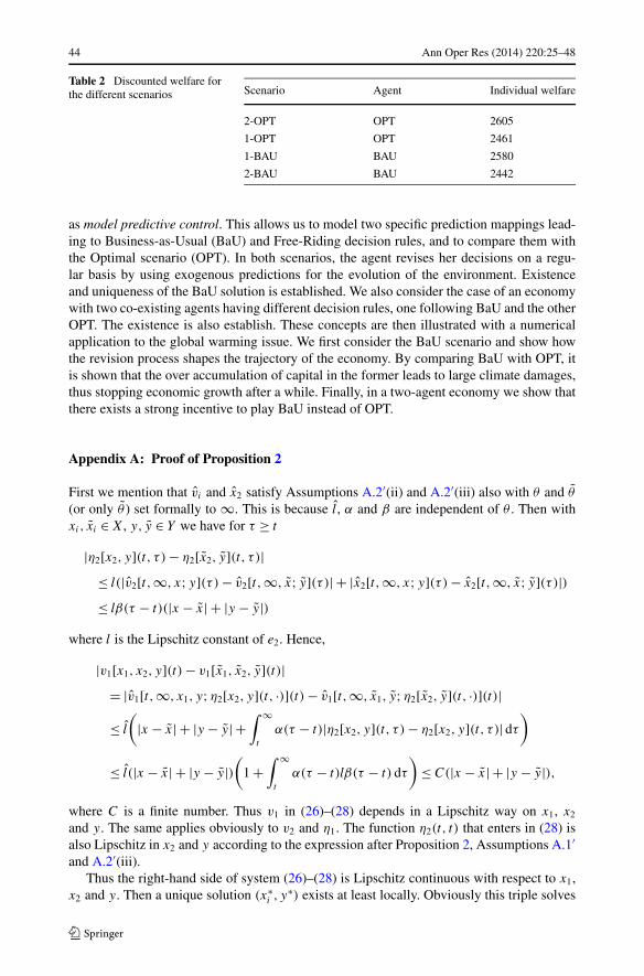
Consumption of an OPT agent in the 2-OPT agent scenario does not dominate the othertrajectories. The 2-BaU scenario provides each agent with a higher consumption from t =30 until t = 110. In a similar way, the OPT (BaU) agent in the 1-OPT, 1-BaU scenarioexhibits higher consumption from t = 20 (25) until t = 70 (90). However, the trajectory ofthe OPT agent in the 2-OPT scenario does provide a higher discounted level of welfare atthe individual (see Table 2), and of course at the aggregate level. When there are 2 OPTagents, the aggregate welfare sums 5210, diminishing to 5041 when there is one OPT andone BaU. Aggregate welfare attains its minimum in the scenario with 2 BaU agents, 4885.This comparison is relative to the time horizon. If we take a longer horizon, the advantageof the 2-OPT scenario over the 2-BaU would be more visible even though the difference isheavily discounted.
6 Conclusion
In this paper we reconsider agents decision rules in an integrated assessment model à laNordhaus. To depart from the standard ill-defined Business-as-Usual scenario we proposealternative—and arguably more realistic—behavioral decision rules. The modeling tech-nique we use adapts ideas from an area in the engendering-oriented control theory, known
44 Ann Oper Res (2014) 220:25–48
Table 2 Discounted welfare forthe different scenarios Scenario Agent Individual welfare
2-OPT OPT 2605
1-OPT OPT 2461
1-BAU BAU 2580
2-BAU BAU 2442
as model predictive control. This allows us to model two specific prediction mappings lead-ing to Business-as-Usual (BaU) and Free-Riding decision rules, and to compare them withthe Optimal scenario (OPT). In both scenarios, the agent revises her decisions on a regu-lar basis by using exogenous predictions for the evolution of the environment. Existenceand uniqueness of the BaU solution is established. We also consider the case of an economywith two co-existing agents having different decision rules, one following BaU and the otherOPT. The existence is also establish. These concepts are then illustrated with a numericalapplication to the global warming issue. We first consider the BaU scenario and show howthe revision process shapes the trajectory of the economy. By comparing BaU with OPT, itis shown that the over accumulation of capital in the former leads to large climate damages,thus stopping economic growth after a while. Finally, in a two-agent economy we show thatthere exists a strong incentive to play BaU instead of OPT.
Appendix A: Proof of Proposition 2
First we mention that vi and x2 satisfy Assumptions A.2′(ii) and A.2′(iii) also with θ and θ
(or only θ ) set formally to ∞. This is because l, α and β are independent of θ . Then withxi, xi ∈ X, y, y ∈ Y we have for τ ≥ t
|η2[x2, y](t, τ ) − η2[x2, y](t, τ )|≤ l(|v2[t,∞, x;y](τ ) − v2[t,∞, x; y](τ )| + |x2[t,∞, x;y](τ ) − x2[t,∞, x; y](τ )|)≤ lβ(τ − t)(|x − x| + |y − y|)
where l is the Lipschitz constant of e2. Hence,
|v1[x1, x2, y](t) − v1[x1, x2, y](t)|= |v1[t,∞, x1, y;η2[x2, y](t, ·)](t) − v1[t,∞, x1, y;η2[x2, y](t, ·)](t)|
≤ l
(|x − x| + |y − y| +
∫ ∞
t
α(τ − t)|η2[x2, y](t, τ ) − η2[x2, y](t, τ )|dτ
)
≤ l(|x − x| + |y − y|)(
1 +∫ ∞
t
α(τ − t)lβ(τ − t) dτ
)≤ C(|x − x| + |y − y|),
where C is a finite number. Thus v1 in (26)–(28) depends in a Lipschitz way on x1, x2
and y. The same applies obviously to v2 and η1. The function η2(t, t) that enters in (28) isalso Lipschitz in x2 and y according to the expression after Proposition 2, Assumptions A.1′and A.2′(iii).
Thus the right-hand side of system (26)–(28) is Lipschitz continuous with respect to x1,x2 and y. Then a unique solution (x∗
i , y∗) exists at least locally. Obviously this triple solves
Ann Oper Res (2014) 220:25–48 45
also (17), (18) with
v∗1(t) = v1[t,∞, x∗
1 (t), y∗(t);η∗2(t, ·)](t), v∗
2(t) = v2[t,∞, x∗2 (t);y∗(t)](t), (A.1)
where
η∗2(t, ·) = e2(·, v2[t,∞, x∗
2 (t);y∗(t)](·), v2[t,∞, x∗2 (t);y∗(t)](·)) = η2[x∗
2 (t), y∗(t)](t, ·).
In particular, Assumption A.1′(ii) implies that (x∗i , y
∗) is extendible to [0,∞).Now we consider an arbitrary pair σ = (h, θ) with h > 0, (ρ−1)θ > h (the last inequality
is not restrictive, since later we shall let h → 0, θ → +∞). We shall compare (x∗i , y
∗) withthe step-wise OPT-BaU solution (vσ
i , xσi , yσ ), corresponding to σ . Denote tσk = kh and
εσk = max
t∈[tσk−1,tσ
k](|(xσ
1 (t) − x∗1 (t)| + |(xσ
2 (t) − x∗2 (t)| + |(yσ (t) − y∗(t)|)
for k = 0,1, . . . , and with tσ−1 redefined as 0.Obviously we have εσ
0 = 0. We shall recurrently estimate εσk+1 by εσ
k . In doing this weuse Assumption A.2′ and the fact that
|x∗1 (t)| + |x∗
2 (t)| + |y∗(t)| ≤ M for every t ≥ 0,
where M is an appropriate constant. Thus for t ∈ [tσk , tσk+1] we have
|xσi (tσk ) − x∗
i (t)| ≤ |xσi (tσk ) − x∗
i (tσk )| + |x∗
i (tσk ) − x∗
i (t)| ≤ εσk + Mh,
and similarly for y.Using Assumption A.2′(iii) and the above inequality we obtain for t ∈ [tσk , tσk+1]
|vσ2 (t) − v∗
2(t)| = |v2[tσk , ρθ, xσ2 (tσk );yσ (tσk )](t) − v2[t,∞, x∗
2 (t);y∗(t)](t)|
≤ β(t − tσk )
[εσk + Mh + δ
(h + 1
tσk + ρθ − t
)]
≤ β(t − tσk )
[εσk + Mh + δ
(h + 1
θ
)]
≤ C1
(εσk + Mh + δ
(h + 1
θ
)),
where C1 is independent of σ . (Obviously one can assume without any restriction that δ
from Assumptions A.2′(ii) and A.2′(iii) is monotone increasing.)Moreover, for τ ∈ [tσk , tσk + θ ] we estimate
|vσ2 (τ ) − v2[t,∞, x∗
2 (t);y∗(t)](τ )|= |v2[tσk , ρθ, xσ
2 (tσk );yσ (tσk )](τ ) − v2[t,∞, x∗2 (t);y∗(t)](τ )|
≤ β(τ − tσk )
[εσk + Mh + δ
(h + 1
tσk + ρθ − τ
)]
≤ β(τ − tσk )
[εσk + Mh + δ
(h + 1
(ρ − 1)θ
)].
46 Ann Oper Res (2014) 220:25–48
In fact, according to Assumption A.2′(iii) the same estimate holds for the sum of the aboveestimated difference and |xσ
2 (τ ) − x2[t,∞, x∗2 (t);y∗(t)](τ )|. Then
|ησ2 (τ ) − η∗
2(t, τ )|= |e2(τ, v
σ2 (τ ), xσ
2 (τ )) − e2(τ, v2[t,∞, x∗2 (t);y∗(t)](τ ), x2[t,∞, x∗
2 (t);y∗(t)](τ ))|
≤ lβ(τ − tσk )
[εσk + Mh + δ
(h + 1
(ρ − 1)θ
)],
where l is the Lipschitz constant of e2. Hence for t ∈ [tσk , tσk+1] we obtain successively
|vσ1 (t) − v∗
1(t)| = |v1[tσk , θ, xσ1 (tσk ), yσ (tσk ); ησ
2 (·)](t) − v1[t,∞, x∗1 (t), y∗(t);η∗
2(t, ·)](t)|
≤ l(εσk + Mh) + δ
(h + 1
θ
)+
∫ tσk
+θ
t
α(τ − tσk )|ησ2 (τ ) − η∗
2(t, τ )|dτ
≤ l(εσk + Mh) + δ
(h + 1
θ
)
+ l
[εσk + Mh + δ
(h + 1
(ρ − 1)θ
)∫ ∞
0α(z)β(z)dz
]
≤ C2
[εσk + h + δ
(h + 1
γ θ
)],
where γ = min{1, ρ − 1} and C2 is independent of σ .Denoting by λ the Lipschitz constant of the overall right-side in (17), (18) with respect
to (vi, xi, y) and C3 = C2 + C3 we obtain in a standard way (using the Grönwall inequality)that
εσk+1 ≤ eλh
[εσk + λC3h
(εσk + h + δ
(h + 1
γ θ
))]
= eλh(1 + λC3h)εσk + eλh
[λC3h
2 + λC3hδ
(h + 1
γ θ
)].
This easily implies (see e.g. Lemma 2.2 in Wolenski 1990) existence of a number C3 (inde-pendent of σ ) such that
εσk ≤ C4e
λkh
[h + δ
(h + 1
γ θ
)]for every k ≥ 0.
Then from the estimations for |vσi (t) − v∗
i (t)| obtained above we conclude that for everyfinite interval [0, T ] one can estimate
|vσi (t) − v∗
i (t)| ≤ CT
[h + δ
(h + 1
γ θ
)]
with CT independent of σ . Hence vσi → v∗
i in C(0,∞) when h → 0, θ → +∞, whichimplies the claim of the proposition.

Ann Oper Res (2014) 220:25–48 47
Appendix B: Discussion of the assumptions
Below we provide a certain justification in the case of the global warming model of theassumptions made in Sects. 3 and 4, focusing on the more requiring Assumptions A.1′and A.2′.
The critical part of Assumption A.1′ is the (uniform in t ) Lipschitz continuity in the setX × X × Y , combined with the invariance of this set with respect to the respective differ-ential equations. Theoretically, due to purely physical arguments, the productivity functionp(t) must be bounded. Hence, according to (2) the capital stock is bounded, therefore theemission is also bounded (since the emission rate e(t) is also bounded). From the stability ofthe atmospheric system (3), (4) the environmental states are also bounded. Hence, the setsX, Y , and E can be specified as bounded sets. Thus the only trouble for the Lipschitz con-tinuity is caused by the unboundedness of our specification for c(a) when a → 1. However,this trouble is artificial—the specification for c(a) is actually relevant only for values of a
far below a = 1. Thus Assumption A.1′ is easily justifiable for the global warming model.The justification of Assumption A.2′ is much more complicated, since it involves the
(unknown) optimal controls v1 and v2. In general, even the uniqueness Assumption A.2′(i)is problematic in the Nordhause type models, as it is shown in Greiner et al. (2009). Namely,in the version of the DICE model considered in Greiner et al. (2009) the authors showexistence of a threshold manifold in the economic-environment state space, starting at whichthe optimal policy is not unique: one leads to “lower warming”, a second one—to a “higherwarming”. However, in that paper the abatement is not used as a control, rather just anexogenous parameter (there are also other small differences in the our model and the onein Greiner et al. 2009). Multiple solutions appear only in the case of a low value of theabatement parameter. Most probably the non-uniqueness disappears when the abatement isused as a second control variable, since the numerical experiments clearly shown uniquenessfor the calibration of the model described in Sect. 5.
Assumption A.2′(iii) is not difficult to check, since v2 is the optimal investment control(the abatement control a obviously equals identically zero) in a version of the Ramsey modelwith a non-stationary but bounded parameter.
Assumption A.2′(ii) is difficult for strict verification. Its claim concerning the dependenceof v1 on θ is an well-know property, but general sufficient conditions for this property are,to our knowledge, not available in the literature. However, it is clear that this property relieson a certain dissipativity, and such is present in our model in a reasonable domain X × Y .
References
Allgöwer, F., & Zheng, A. (2000). Progress in systems theory: Vol. 26. Nonlinear model predictive control.Basel: Birkhäuser.
Bréchet, Th., Eyckmans, J., Gerard, F., Marbaix, Ph., Tulkens, H., & van Ypersele, J.-P. (2010). The impactof the unilateral EU commitment on the stability of international climate agreements. Climate Policy,10, 148–166.
Bréchet, Th., Gerard, F., & Tulkens, H. (2011). Efficiency vs. stability of climate coalitions: a conceptual andcomputational appraisal. The Energy Journal, 32(1), 49–76.
Bosetti, V., Carraro, C., De Cian, E., Duval, R., Massetti, E., & Tavoni, M. (2009). The incentives to partici-pate in, and the stability of, international climate coalitions: a game-theoretic analysis using the Witchmodel. 2009.064 Note di lavoro, FEEM.
Carlson, D. A., Haurie, A. B., & Leizarowitz, A. (1991). Infinite horizon optimal control. Berlin: Springer.Diehl, M., Bock, H. G., Schilder, J. P., Findeisen, R., Nagy, Z., & Allgöwer, F. (2002). Real-time optimiza-
tion and nonlinear model predictive control of processes governed by differential-algebraic equations.Journal of Process Control, 12, 577–585.

48 Ann Oper Res (2014) 220:25–48
Dontchev, A. L., & Rockafellar, R. T. (2009). Springer monographs in mathematics. Implicit functions andsolution mappings. A view from variational analysis. Berlin: Springer.
Eyckmans, J., & Tulkens, H. (2003). Simulating coalitionally stable burden sharing agreements for the climatechange problem. Resource and Energy Economics, 25, 299–327.
Findeisen, R., Allgöwer, F., & Biegler, L. T. (Eds.) (2007). Lecture notes in control and information sciences:Vol. 358. Assessment and future directions of nonlinear model predictive control. Berlin: Springer.
Greiner, A., & Semmler, W. (2005). Economic growth and global warming: a model of multiple equilibriaand thresholds. Journal of Economic Behavior and Organization, 57, 430–447.
Greiner, A., Grüne, L., & Semmler, W. (2009). Growth and climate change: threshold and multiple equilibria.In J. Crespo Cuaresma, T. Palokangas, & A. Tarasyev (Eds.), Dynamic modeling and econometrics ineconomics and finance: Vol. 12. Dynamic systems, economic growth, and the environment (pp. 63–78).Berlin: Springer. ISBN:978-3-642-02131-2.
Haurie, A. (2003). Integrated assessment modeling for global climate change: an infinite horizon optimizationviewpoint. Environmental Modeling and Assessment, 8, 117–132.
Haurie, A. (2005). A multigenerational game model to analyze sustainable development. Annals of Opera-tional Research, 137, 369–386.
Kriegler, E., Hall, J. W., Held, H., Dawson, R., & Schellnhuber, H. J. (2009). Imprecise probability assess-ment of tipping points in the climate system. Proceedings of the National Academy of Sciences, 106,5041–5046.
Nordhaus, W. D. (1992). An optimal transition path for controlling greenhouse gases. Science, 258(5086),1315–1319.
Nordhaus, W. D. (1993). Rolling the DICE: an optimal transition path for controlling greenhouse gases.Resource and Energy Economics, 15, 27–50.
Nordhaus, W. D. (1993). Optimal greenhouse gas reductions and tax policy in the DICE model. The AmericanEconomic Review, 83, 313–317.
Nordhaus, W. D. (2008). A question of balance: economic modeling of global warming. New Haven: YaleUniversity Press.
Nordhaus, W. D., & Boyer, J. (2000). Warming the world. Cambridge: MIT Press.Solomon, S., Qin, D., Manning, M., Chen, Z., Marquis, M., Averyt, K. B., Tignor, M., & Miller, H. L. (Eds.)
(2007). Contribution of working group I to the fourth assessment report of the intergovernmental panelon climate change. Cambridge: Cambridge University Press.
Stern, N. (2006). The economics of climate change: the Stern review. Cambridge: Cambridge UniversityPress.
Yang, Z. (2008). Strategic bargaining and cooperation in greenhouse gas mitigations—an integrated assess-ment modeling approach. Cambridge: MIT Press.
Wolenski, P. (1990). The exponential formula for the reachable set of Lipschitz differential inclusion. SIAMJournal on Control and Optimization, 28, 1148–1161.