model predictive control toolbox - instructional web...
TRANSCRIPT

For Use with MATLAB®
User’s GuideVersion 2
Model Predictive ControlToolbox
Alberto BemporadManfred Morari
N. Lawrence Ricker
How to Contact The MathWorks:
www.mathworks.com Webcomp.soft-sys.matlab Newsgroup
[email protected] Technical [email protected] Product enhancement [email protected] Bug [email protected] Documentation error [email protected] Order status, license renewals, [email protected] Sales, pricing, and general information
508-647-7000 Phone
508-647-7001 Fax
The MathWorks, Inc. Mail3 Apple Hill DriveNatick, MA 01760-2098
For contact information about worldwide offices, see the MathWorks Web site.
Model Predictive Control Toolbox User’s Guide © COPYRIGHT 1995-2005 by The MathWorks, Inc. The software described in this document is furnished under a license agreement. The software may be used or copied only under the terms of the license agreement. No part of this manual may be photocopied or repro-duced in any form without prior written consent from The MathWorks, Inc.
FEDERAL ACQUISITION: This provision applies to all acquisitions of the Program and Documentation by, for, or through the federal government of the United States. By accepting delivery of the Program or Documentation, the government hereby agrees that this software or documentation qualifies as commercial computer software or commercial computer software documentation as such terms are used or defined in FAR 12.212, DFARS Part 227.72, and DFARS 252.227-7014. Accordingly, the terms and conditions of this Agreement and only those rights specified in this Agreement, shall pertain to and govern the use, modification, reproduction, release, performance, display, and disclosure of the Program and Documentation by the federal government (or other entity acquiring for or through the federal government) and shall supersede any conflicting contractual terms or conditions. If this License fails to meet the government's needs or is inconsistent in any respect with federal procurement law, the government agrees to return the Program and Documentation, unused, to The MathWorks, Inc.
MATLAB, Simulink, Stateflow, Handle Graphics, Real-Time Workshop, and xPC TargetBox are registered trademarks of The MathWorks, Inc.
Other product or brand names are trademarks or registered trademarks of their respective holders.Printing History: January 1995 First printing
October 1998 Online onlyJune 2004 Online only Revised for Version 2.0 (Release 14)October 2004 Online only Revised for Version 2.1 (Release 14SP1)March 2005 Online only Revised for Version 2.2 (Release 14SP2)

Contents
1Introduction
What Is the Model Predictive Control Toolbox? . . . . . . . . . . 1-2
Model Predictive Control of a SISO Plant . . . . . . . . . . . . . . . 1-3A Typical Sampling Instant . . . . . . . . . . . . . . . . . . . . . . . . . . . . 1-5Prediction and Control Horizons . . . . . . . . . . . . . . . . . . . . . . . . 1-8
MIMO Plants . . . . . . . . . . . . . . . . . . . . . . . . . . . . . . . . . . . . . . . . 1-10Optimization and Constraints . . . . . . . . . . . . . . . . . . . . . . . . . 1-10State Estimation . . . . . . . . . . . . . . . . . . . . . . . . . . . . . . . . . . . . 1-13Blocking . . . . . . . . . . . . . . . . . . . . . . . . . . . . . . . . . . . . . . . . . . . 1-14
2MPC Problem Setup
Prediction Model . . . . . . . . . . . . . . . . . . . . . . . . . . . . . . . . . . . . . 2-2Offsets . . . . . . . . . . . . . . . . . . . . . . . . . . . . . . . . . . . . . . . . . . . . . 2-4
Optimization Problem . . . . . . . . . . . . . . . . . . . . . . . . . . . . . . . . . 2-5
State Estimation . . . . . . . . . . . . . . . . . . . . . . . . . . . . . . . . . . . . . . 2-8Measurement Noise Model . . . . . . . . . . . . . . . . . . . . . . . . . . . . . 2-8Output Disturbance Model . . . . . . . . . . . . . . . . . . . . . . . . . . . . . 2-9State Observer . . . . . . . . . . . . . . . . . . . . . . . . . . . . . . . . . . . . . . . 2-9
QP Matrices . . . . . . . . . . . . . . . . . . . . . . . . . . . . . . . . . . . . . . . . . 2-12Prediction . . . . . . . . . . . . . . . . . . . . . . . . . . . . . . . . . . . . . . . . . . 2-12Optimization Variables . . . . . . . . . . . . . . . . . . . . . . . . . . . . . . . 2-13Cost Function . . . . . . . . . . . . . . . . . . . . . . . . . . . . . . . . . . . . . . . 2-15Constraints . . . . . . . . . . . . . . . . . . . . . . . . . . . . . . . . . . . . . . . . 2-16
MPC Computation . . . . . . . . . . . . . . . . . . . . . . . . . . . . . . . . . . . 2-18
i

ii Contents
Unconstrained MPC . . . . . . . . . . . . . . . . . . . . . . . . . . . . . . . . . . 2-18Constrained MPC . . . . . . . . . . . . . . . . . . . . . . . . . . . . . . . . . . . . 2-18
Using Identified Models . . . . . . . . . . . . . . . . . . . . . . . . . . . . . . 2-19
3MPC Simulink Library
MPC Controller Block . . . . . . . . . . . . . . . . . . . . . . . . . . . . . . . . . 3-2Opening the Library . . . . . . . . . . . . . . . . . . . . . . . . . . . . . . . . . . 3-2MPC Controller Block Mask . . . . . . . . . . . . . . . . . . . . . . . . . . . . 3-3Look Ahead and Signals from the Workspace . . . . . . . . . . . . . . 3-4Initialization . . . . . . . . . . . . . . . . . . . . . . . . . . . . . . . . . . . . . . . . . 3-5Using the MPC Toolbox with Real-Time Workshop® . . . . . . . . 3-5
4Case-Study Examples
Servomechanism Controller . . . . . . . . . . . . . . . . . . . . . . . . . . . 4-2System Model . . . . . . . . . . . . . . . . . . . . . . . . . . . . . . . . . . . . . . . . 4-2Control Objectives and Constraints . . . . . . . . . . . . . . . . . . . . . . 4-4Defining the Plant Model . . . . . . . . . . . . . . . . . . . . . . . . . . . . . . 4-4Controller Design Using MPCTOOL . . . . . . . . . . . . . . . . . . . . . 4-5Using MPC Toolbox Commands . . . . . . . . . . . . . . . . . . . . . . . . 4-22Using MPC Tools in Simulink . . . . . . . . . . . . . . . . . . . . . . . . . . 4-26
Paper Machine Process Control . . . . . . . . . . . . . . . . . . . . . . . 4-30Linearizing the Nonlinear Model . . . . . . . . . . . . . . . . . . . . . . . 4-31MPC Design . . . . . . . . . . . . . . . . . . . . . . . . . . . . . . . . . . . . . . . . 4-33Controlling the Nonlinear Plant in Simulink . . . . . . . . . . . . . . 4-39
Reference . . . . . . . . . . . . . . . . . . . . . . . . . . . . . . . . . . . . . . . . . . . 4-43

5The Design Tool
Opening the MPC Design Tool . . . . . . . . . . . . . . . . . . . . . . . . . . 5-2
The Menu Bar . . . . . . . . . . . . . . . . . . . . . . . . . . . . . . . . . . . . . . . . 5-3File Menu . . . . . . . . . . . . . . . . . . . . . . . . . . . . . . . . . . . . . . . . . . . 5-3MPC Menu . . . . . . . . . . . . . . . . . . . . . . . . . . . . . . . . . . . . . . . . . . 5-4
The Tool Bar . . . . . . . . . . . . . . . . . . . . . . . . . . . . . . . . . . . . . . . . . . 5-6
The Tree View . . . . . . . . . . . . . . . . . . . . . . . . . . . . . . . . . . . . . . . . 5-7Node Types . . . . . . . . . . . . . . . . . . . . . . . . . . . . . . . . . . . . . . . . . . 5-7Renaming a Node . . . . . . . . . . . . . . . . . . . . . . . . . . . . . . . . . . . . . 5-8
Importing a Plant Model . . . . . . . . . . . . . . . . . . . . . . . . . . . . . . . 5-9Import from . . . . . . . . . . . . . . . . . . . . . . . . . . . . . . . . . . . . . . . . 5-10Import to . . . . . . . . . . . . . . . . . . . . . . . . . . . . . . . . . . . . . . . . . . . 5-11Buttons . . . . . . . . . . . . . . . . . . . . . . . . . . . . . . . . . . . . . . . . . . . . 5-11Importing a Linearized Plant Model . . . . . . . . . . . . . . . . . . . . . 5-12
Importing a Controller . . . . . . . . . . . . . . . . . . . . . . . . . . . . . . . 5-15Import from . . . . . . . . . . . . . . . . . . . . . . . . . . . . . . . . . . . . . . . . 5-16Import to . . . . . . . . . . . . . . . . . . . . . . . . . . . . . . . . . . . . . . . . . . . 5-17Buttons . . . . . . . . . . . . . . . . . . . . . . . . . . . . . . . . . . . . . . . . . . . . 5-17
Exporting a Controller . . . . . . . . . . . . . . . . . . . . . . . . . . . . . . . 5-19Dialog Options . . . . . . . . . . . . . . . . . . . . . . . . . . . . . . . . . . . . . . 5-19Buttons . . . . . . . . . . . . . . . . . . . . . . . . . . . . . . . . . . . . . . . . . . . . 5-20
Signal Definition View . . . . . . . . . . . . . . . . . . . . . . . . . . . . . . . . 5-21MPC Structure Overview . . . . . . . . . . . . . . . . . . . . . . . . . . . . . 5-22Buttons . . . . . . . . . . . . . . . . . . . . . . . . . . . . . . . . . . . . . . . . . . . . 5-22Signal Properties Tables . . . . . . . . . . . . . . . . . . . . . . . . . . . . . . 5-22Right-Click Menu Options . . . . . . . . . . . . . . . . . . . . . . . . . . . . . 5-25
Plant Models View . . . . . . . . . . . . . . . . . . . . . . . . . . . . . . . . . . . 5-26Plant Models List . . . . . . . . . . . . . . . . . . . . . . . . . . . . . . . . . . . . 5-27Model Details . . . . . . . . . . . . . . . . . . . . . . . . . . . . . . . . . . . . . . . 5-27Additional Notes . . . . . . . . . . . . . . . . . . . . . . . . . . . . . . . . . . . . 5-28
iii

iv Contents
Buttons . . . . . . . . . . . . . . . . . . . . . . . . . . . . . . . . . . . . . . . . . . . . 5-28Right-Click Options . . . . . . . . . . . . . . . . . . . . . . . . . . . . . . . . . . 5-28
Controllers View . . . . . . . . . . . . . . . . . . . . . . . . . . . . . . . . . . . . . 5-29Controllers List . . . . . . . . . . . . . . . . . . . . . . . . . . . . . . . . . . . . . 5-30Controller Details . . . . . . . . . . . . . . . . . . . . . . . . . . . . . . . . . . . . 5-31Additional Notes . . . . . . . . . . . . . . . . . . . . . . . . . . . . . . . . . . . . 5-31Buttons . . . . . . . . . . . . . . . . . . . . . . . . . . . . . . . . . . . . . . . . . . . . 5-31Right-Click Options . . . . . . . . . . . . . . . . . . . . . . . . . . . . . . . . . . 5-32
Simulation Scenarios List . . . . . . . . . . . . . . . . . . . . . . . . . . . . . 5-33Scenarios List . . . . . . . . . . . . . . . . . . . . . . . . . . . . . . . . . . . . . . . 5-34Scenario Details . . . . . . . . . . . . . . . . . . . . . . . . . . . . . . . . . . . . . 5-35Additional Notes . . . . . . . . . . . . . . . . . . . . . . . . . . . . . . . . . . . . 5-35Buttons . . . . . . . . . . . . . . . . . . . . . . . . . . . . . . . . . . . . . . . . . . . . 5-35Right-Click Options . . . . . . . . . . . . . . . . . . . . . . . . . . . . . . . . . . 5-35
Controller Specifications View . . . . . . . . . . . . . . . . . . . . . . . . 5-36Model and Horizons Tab . . . . . . . . . . . . . . . . . . . . . . . . . . . . . . 5-36Constraints Tab . . . . . . . . . . . . . . . . . . . . . . . . . . . . . . . . . . . . . 5-40Constraint Softening . . . . . . . . . . . . . . . . . . . . . . . . . . . . . . . . . 5-43Weight Tuning Tab . . . . . . . . . . . . . . . . . . . . . . . . . . . . . . . . . . 5-47Estimation Tab . . . . . . . . . . . . . . . . . . . . . . . . . . . . . . . . . . . . . . 5-50Right-Click Menus . . . . . . . . . . . . . . . . . . . . . . . . . . . . . . . . . . . 5-58
Simulation Scenario View . . . . . . . . . . . . . . . . . . . . . . . . . . . . 5-59Simulation Settings . . . . . . . . . . . . . . . . . . . . . . . . . . . . . . . . . . 5-60Setpoints . . . . . . . . . . . . . . . . . . . . . . . . . . . . . . . . . . . . . . . . . . . 5-60Measured Disturbances . . . . . . . . . . . . . . . . . . . . . . . . . . . . . . . 5-61Unmeasured Disturbances . . . . . . . . . . . . . . . . . . . . . . . . . . . . 5-62Signal Type Settings . . . . . . . . . . . . . . . . . . . . . . . . . . . . . . . . . 5-64Simulation Button . . . . . . . . . . . . . . . . . . . . . . . . . . . . . . . . . . . 5-65Right-Click Menus . . . . . . . . . . . . . . . . . . . . . . . . . . . . . . . . . . . 5-65
Response Plots . . . . . . . . . . . . . . . . . . . . . . . . . . . . . . . . . . . . . . . 5-67Data Markers . . . . . . . . . . . . . . . . . . . . . . . . . . . . . . . . . . . . . . . 5-67Displaying Multiple Scenarios . . . . . . . . . . . . . . . . . . . . . . . . . 5-69Viewing Selected Variables . . . . . . . . . . . . . . . . . . . . . . . . . . . . 5-70Grouping Variables in a Single Plot . . . . . . . . . . . . . . . . . . . . . 5-70
Normalizing Response Amplitudes . . . . . . . . . . . . . . . . . . . . . . 5-71
6Function Reference
Functions — Categorical List . . . . . . . . . . . . . . . . . . . . . . . . . . 6-2MPC Controller . . . . . . . . . . . . . . . . . . . . . . . . . . . . . . . . . . . . . . 6-2MPC Controller Characteristics . . . . . . . . . . . . . . . . . . . . . . . . . 6-2Linear Behavior of MPC Controller . . . . . . . . . . . . . . . . . . . . . . 6-3MPC State . . . . . . . . . . . . . . . . . . . . . . . . . . . . . . . . . . . . . . . . . . 6-3MPC Computation and Simulation . . . . . . . . . . . . . . . . . . . . . . . 6-3State Estimation . . . . . . . . . . . . . . . . . . . . . . . . . . . . . . . . . . . . . 6-4Quadratic Programming . . . . . . . . . . . . . . . . . . . . . . . . . . . . . . . 6-4
Functions — Alphabetical List . . . . . . . . . . . . . . . . . . . . . . . . . 6-5
7Block Reference
Blocks — Alphabetical List . . . . . . . . . . . . . . . . . . . . . . . . . . . . . 7-2
8Object Reference
MPC Controller Object . . . . . . . . . . . . . . . . . . . . . . . . . . . . . . . . 8-2Construction and Initialization . . . . . . . . . . . . . . . . . . . . . . . . . 8-12
MPC State Object . . . . . . . . . . . . . . . . . . . . . . . . . . . . . . . . . . . . 8-13
MPC Simulation Options Object . . . . . . . . . . . . . . . . . . . . . . . 8-14
v

vi Contents
Index
1
Introduction
What Is the Model Predictive Control Toolbox? (p. 1-2) Toolbox overview
Model Predictive Control of a SISO Plant (p. 1-3) Toolbox concepts: horizons, constraints, tuning weights
MIMO Plants (p. 1-10) Extension to plants with multiple inputs and outputs
1 Introduction
1-2
What Is the Model Predictive Control Toolbox?The Model Predictive Control (MPC) Toolbox is a collection of software that helps you design, analyze, and implement an advanced industrial automation algorithm. Like other MATLAB® tools, it provides a convenient graphical user interface (GUI) as well as a flexible command syntax that supports customization.
As its name suggests, MPC automates a target system (the “plant”) by combining a prediction and a control strategy. An approximate, linear plant model provides the prediction. The control strategy compares predicted plant states to a set of objectives, then adjusts available actuators to achieve the objectives while respecting the plant’s constraints. Such constraints can include the actuators’ physical limits, boundaries of safe operation, and lower limits for product quality.
MPC’s constraint-tolerance differentiates it from other “optimal control” strategies (e.g., the Linear-Quadratic-Gaussian approach supported in the Control Systems Toolbox). The impetus for this is industrial experience suggesting that the drive for profitability often pushes the plant to one or more constraints. MPC’s explicit consideration of such factors allows it to allocate the available plant resources intelligently as the system evolves over time.
The MPC Toolbox uses the same powerful linear dynamic modeling tools found in the Control Systems and System Identification Toolboxes. You can employ transfer functions, state-space matrices, or a combination of the two. You can also include delays, which are a common feature of industrial plants.
If you don’t have a model but can perform experiments, you can use the System Identification Toolbox to develop a data-based model, then exploit it in the MPC Toolbox.
If you’d rather use Simulink® graphical tools to model your plant, the MPC Toolbox provides a Simulink block for that environment. For example, you can easily linearize a nonlinear Simulink plant, use the linearized model to build an MPC Controller block, and evaluate its control of the nonlinear plant.
Finally,you can use MPC tools in Simulink to develop and test a control strategy, then implement it in a real plant using the Real Time Workshop.

Model Predictive Control of a SISO Plant
Model Predictive Control of a SISO PlantThe usual MPC Toolbox application involves a plant having multiple inputs and multiple outputs (a MIMO plant).
Consider instead the simpler application shown in Figure 1-1 (see summary of nomenclature in Table 1-1). This plant could be a manufacturing process, such as a unit operation in an oil refinery, or a device, such as an electric motor. The main objective is to hold a single output, , at a reference value (or setpoint), r, by adjusting a single manipulated variable (or actuator) u. This is what is generally termed a SISO (single-input single-output) plant. The block labeled MPC represents an MPC Toolbox feedback controller designed to achieve the control objective.
The SISO plant actually has multiple inputs, as shown in Figure 1-1. In addition to the manipulated variable input, u, there may be a measured disturbance, v, and an unmeasured disturbance, d.
Figure 1-1: Block Diagram of a SISO MPC Toolbox Application
The unmeasured disturbance is always present. As shown in Figure 1-1, it is an independent input – not affected by the controller or the plant. It represents all the unknown, unpredictable events that upset plant operation. (In the context of Model Predictive Control, it can also represent unmodeled dynamics.) When such an event occurs, the only indication is its effect on the measured output, y, which is fed back to the controller as shown in Figure 1-1.
y
++PlantMPC
v
r
yd
z
yyu
v
Measured Disturbance
Measured Output (Controlled Variable)
Noise
Setpoint
UnmeasuredDisturbance
ActuatorPlantOutput
1-3

1 Introduction
1-4
Some applications have unmeasured disturbances only. A measured disturbance, v, is another independent input affecting . In contrast to d, the controller receives the measured v directly, as shown in Figure 1-1 This allows the controller to compensate for v’s impact on immediately rather than waiting until the effect appears in the y measurement. This is called feedforward control.
In other words, an MPC Toolbox design always provides feeback compensation for unmeasured disturbances and feedforward compensation for any measured disturbance.
Table 1-1: Description of MPC Toolbox Signals
Symbol Description
d Unmeasured disturbance. Unknown but for its effect on the plant output. The controller provides feedback compensation for such disturbances.
r Setpoint (or reference). The target value for the output.
u Manipulated variable(or actuator). The signal the controller adjusts in order to achieve its objectives.
v Measured disturbance (optional). The controller provides feedforward compensation for such disturbances as they occur to minimize their impact on the output.
Output (or controlled variable). The signal to be held at the setpoint. This is the “true” value, uncorrupted by measurement noise.
y Measured output. Used to estimate the true value, .
z Measurement noise. Represents electrical noise, sampling errors, drifting calibration, and other effects that impair measurement precision and accuracy.
y
y
y
y

Model Predictive Control of a SISO Plant
The MPC Toolbox design requires a model of the impact that v and u have on (symbolically, and ). It uses this plant model to calculate the u
adjustments needed to keep at its setpoint.
This calculation considers the effect of any known constraints on the adjustments (typically an actuator upper or lower bound, or a constraint on how rapidly u can vary). One may also specify bounds on . These constraint specifications are a distinguishing feature of an MPC Toolbox design and can be particularly valuable when one has multiple control objectives to be achieved via multiple adjustments (a MIMO plant). In the context of a SISO system, such contraint handling is often termed an anti-windup feature.
If the plant model is accurate, the plant responds quickly to adjustments in u, and no constraints are encountered, feedforward compensation can counteract the impact of v perfectly. In reality, model imperfections, physical limitations, and unmeasured disturbances cause the y to deviate from its setpoint. Therefore, the MPC Toolbox design includes a disturbance model ( ) to estimate d and predict its impact on . It then uses its model to calculate appropriate adjustments (feedback). This calculation also considers the known constraints.
Various noise effects can corrupt the measurement. The signal z in Figure 1-1 represents such effects. They could vary randomly with a zero mean, or could exhibit a non-zero, drifting bias. The MPC Toolbox design uses a model in combination with its model to remove the estimated noise component (filtering).
The above feedforward/feedback actions comprise the controller’s regulator mode. The MPC Toolbox design also provides a servo mode, i.e., it adjusts u such that tracks a time-varying setpoint.
The tracking accuracy depends on the plant characteristics (including constraints), the accuracy of the model, and whether or not future setpoint variations can be anticipated, i.e., known in advance. If so, it provides feedforward compensation for these.
A Typical Sampling InstantAn MPC Toolbox design generates a discrete-time controller – one that takes action at regularly-spaced, discrete time instants. The sampling instants are the times at which the controller acts. The interval separating successive sampling instants is the sampling period, ∆t (also called the control interval).
y v y→ u y→y
y
d y→y u y→
z y→d y→
y
u y→
1-5
1 Introduction
1-6
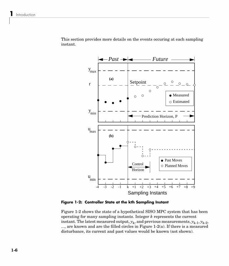
This section provides more details on the events occuring at each sampling instant.
Figure 1-2: Controller State at the kth Sampling Instant
Figure 1-2 shows the state of a hypothetical SISO MPC system that has been operating for many sampling instants. Integer k represents the current instant. The latest measured output, yk, and previous measurements, yk-1, yk-2, ..., are known and are the filled circles in Figure 1-2(a). If there is a measured disturbance, its current and past values would be known (not shown).
y
ymin
max
Setpoint
Past Future
EstimatedMeasured
Prediction Horizon, P
r
Sampling Instants
umin
umax
ControlHorizon
Past MovesPlanned Moves
k +1 +2 +3 +4 +5 +6 +7 +8 +9-1-2-3-4
(a)
(b)

Model Predictive Control of a SISO Plant
Figure 1-2 (b) shows the controller’s previous moves, uk-41, ..., uk-1, as filled circles. As is usually the case, a zero-order hold receives each move from the controller and holds it until the next sampling instant, causing the step-wise variations shown in Figure 1-2 (b).
To calculate its next move, uk the controller operates in two phases:
1 Estimation. In order to make an intelligent move, the controller needs to know the current state. This includes the true value of the controlled variable, , and any internal variables that influence the future trend,
, ..., . To accomplish this, the controller uses all past and current measurements and the models , , , and . For details, see “Prediction” and “State Estimation”.
2 Optimization. Values of setpoints, measured disturbances, and constraints are specified over a finite horizon of future sampling instants, k+1, k+2, ..., k+P, where P (a finite integer ≥ 1) is the prediction horizon – see Figure 1-2 (a). The controller computes M moves uk, uk+1, ... uk+M-1, where M ( ≥ 1, ≤ P) is the control horizon – see Figure 1-2 (b). In the hypothetical example shown in the figure, P = 9 and M = 4. The moves are the solution of a constrained optimization problem. For details of the formulation, see Chapter 2, “Optimization Problem”.
In the example, the optimal moves are the four open circles in Figure 1-2 (b), and the controller predicts that the resulting output values will be the nine open circles in Figure 1-2 (a). Notice that both are within their constraints,
and .
When it’s finished calculating, the controller sends move uk to the plant. The plant operates with this constant input until the next sampling instant, ∆t time units later. The controller then obtains new measurements and totally revises its plan. This cycle repeats indefinitely.
Reformulation at each sampling instant is essential for good control. The predictions made during the optimization stage are imperfect. Periodic measurement feedback allows the controller to correct for this error and for unexpected disturbances.
ykyk 1+ yk P+
u y→ d y→ w y→ z y→
umin uk j+ umax≤ ≤ ymin yk i+ ymax≤ ≤
1-7

1 Introduction
1-8
Prediction and Control HorizonsYou might wonder why the controller bothers to optimize over P future sampling periods and calculate M future moves when it discards all but the first move in each cycle. Indeed, under certain conditions a controller using P = M = 1 would be identical to one using P = M = ∞. More often, however, the horizon values have an important impact. Some examples follow:
• Constraints. Given sufficiently long horizons, the controller can “see” a potential constraint and avoid it – or at least minimize its adverse effects. For example, consider the situation depicted below in which one controller objective is to keep plant output y below an upper bound ymax. The current sampling instant is k, and the model predicts the upward trend yk+i. If the controller were looking P1 steps ahead, it wouldn’t be concerned by the constraint until more time had elapsed. If the prediction horizon were P2, it would begin to take corrective action immediately.
• Plant delays. Suppose that the plant includes a pure time delay equivalent to D sampling instants. In other words, the controller’s current move, uk, has no effect until yk+D+1. In this situation it is essential that P >> D and M << P − D, as this forces the controller to consider the full effect of each move.
For example, suppose D = 5, P = 7, M = 3, the current time instant is k, and the three moves to be calculated are uk, uk+1, and uk+2. Moves uk, uk+1 would have some impact within the prediction horizon, but move uk+2 would have none until yk+8, which is outside. Thus, uk+2 is indeterminant. Setting P = 8 (or M = 2) would allow a unique value to be determined. It would be better to increase P even more.
• Other nonminimum phase plants. Consider a SISO plant with an inverse-response, i.e., a plant with a short-term response in one direction,
k k+P1 k+P2
ymax
yk+i

Model Predictive Control of a SISO Plant
but a longer term response in the opposite direction. The optimization should focus primarily on the longer-term behavior. Otherwise, the controller would move in the wrong direction.
Most designers choose P and M such that controller performance is insensitive to small adjustments in these horizons. Here are typical rules of thumb for a lag-dominant, stable process:
1 Choose the control interval such that the plant’s open-loop settling time is approximately 20-30 sampling periods (i.e., the sampling period is approximately one fifth of the dominant time constant).
2 Choose prediction horizon P to be the number of sampling periods used in step 1.
3 Use a relatively small control horizon M, e.g., 3-5.
If performance is poor, you should examine other aspects of the optimization problem and/or check for inaccurate controller predictions.
1-9

1 Introduction
1-1
MIMO PlantsOne advantage of an MPC Toolbox design (relative to classical multi-loop control) is that it generalizes directly to plants having multiple inputs and outputs. Moreover, the plant can be non-square, i.e., having an unequal number of actuators and outputs. Industrial applications involving hundreds of actuators and controller outputs have been reported.
The main challenge is to tune the controller to achieve multiple objectives. For example, if there are several outputs to be controlled, it might be necessary to prioritize so that the controller provides accurate setpoint tracking for the most important output, sacrificing others when necessary, e.g., when it encounters constraints. The MPC Toolbox features support such prioritization.
Optimization and ConstraintsAs discussed in more detail in Chapter 2, “Optimization Problem”, the MPC Toolbox controller solves anoptimization problem much like the LQG optimal control described in the Control System Toolbox. The main difference is that the MPC Toolbox optimization problem includes explicit constraints on u and y.
Setpoint TrackingConsider first a case with no constraints. A primary control objective is to force the plant outputs to track their setpoints.
Specifically, the controller predicts how much each output will deviate from its setpoint within the prediction horizon. It multiplies each deviation by the output’s weight, and computes the weighted sum of squared deviations, , as follows:
where k is the current sampling interval, k+i is a future sampling interval (within the prediction horizon), P is the prediction horizon, ny is the number of plant outputs, is the weight for output j, and is the predicted deviation at future instant k+i.
If the controller does its best to track rj, sacrificing ri tracking if necessary. If , on the other hand, the controller completely ignores deviations rj–yj.
Sy k( )
Sy k( ) wyj rj k i+( ) yj k i+( )–[ ]
⎩ ⎭⎨ ⎬⎧ ⎫
j 1=
ny
∑i 1=
P
∑=
wjy rj k i+( ) yj k i+( )–[ ]
wjy wi j≠
y»wj
y 0=
0

MIMO Plants
Choosing the weights is a critical step. You will usually need to tune your controller, varying the weights to achieve the desired behavior.
As an example, consider Figure 1-3, which depicts a type of chemical reactor (a CSTR). Feed enters continuously with reactant concentration CAi. A reaction takes place inside the vessel at temperature T. Product exits continuously, and contains residual reactant at concentration CA (<CAi).
The reaction liberates heat. A coolant having temperature Tc flows through coils immersed in the reactor to remove excess heat.
Figure 1-3: CSTR Schematic
From the MPC Toolbox point for view, T and CA would be plant outputs, and CAi and Tc would be inputs. More specifically, CAi would be an independent disturbance input, and Tc would be a manipulated variable (actuator).
There is one manipulated variable (the coolant temperature), so it’s impossible to hold both T and CA at setpoints. Controlling T would usually be a high priority. Thus, you might set the output weight for T much larger than that for CA. In fact, you might set the CA weight to zero, allowing CA to float within an acceptable operating region (to be defined by constraints).
Move SuppressionIf the controller focuses exclusively on setpoint tracking, it might choose to make large manipulated-variable adjustments. These could be impossible to achieve. They could also accelerate equipment wear or lead to control system instability.
Thus, the MPC Toolbox controller also monitors a weighted sum of controller adjustments, calculated according to the following equation:
Tc
CAi
CAT
1-11

1 Introduction
1-1
where M is the control horizon, nmv is the number of manipulated variables, is the predicted adjustment (i.e., move) in manipulated variable
j at future (or current) sampling interval , and is a weight, which must be zero or positive. Increasing forces the controller to make smaller, more cautious moves. In many cases (but not all) this will have the following effects:
• The controller’s setpoint tracking will degrade
• The controller will be less sensitive to prediction inaccuracies (i.e., more robust)
Setpoints on Manipulated VariablesIn most applications, the controller’s manipulated variables (MVs) should move freely (within a constrained region) to compensate for disturbances and stepoint changes. An attempt to hold an MV at a point within the region would degrade output setpoint tracking.
On the other hand, some plants have more MVs than output setpoints. In such a plant, if all manipulated variables were allowed to move freely, the MV values needed to achieve a particular setpoint or to reject a particular disturbance would be non-unique. Thus, the MVs would drift within the operating space.
A common approach is to define setpoints for “extra” MVs. These setpoints usually represent operating conditions that improve safety, economic return, etc. The MPC Toolbox design includes an additional term to accommodate such cases, as follows:
where is the manipulated variable setpoint (nominal value) for the jth MV, and is the corresponding weight.
S∆u k( ) wj∆u∆uj k i 1–+( )
⎩ ⎭⎨ ⎬⎧ ⎫
2
j 1=
nmv
∑i 1=
M
∑=
∆uj k i 1–+( )k i 1–+ wj
∆u
wj∆u
∆uj
Su k( ) wju uj uj k i 1–+( )–[ ]
⎩ ⎭⎨ ⎬⎧ ⎫
j 1=
nmv
∑i 1=
M
∑=
ujwj
u
2

MIMO Plants
ConstraintsConstraints may be either hard or soft. A hard constraint must not be violated. Unfortunately, under some conditions a constraint violation might be unavoidable (e.g., an unexpected, large disturbance), and a realistic controller must allow for this.
The MPC Toolbox does so by softening each constraint, making a violation mathematically acceptable, though discouraged. The designer may specify the degree of softness in each case, making selected constraints less likely to be violated than others. See “Optimization Problem” on page 2-5 for the mathematical details.
Briefly, you specify a tolerance band for each constraint. If the tolerance band is zero, the constraint is hard (no violation allowed). Increasing the tolerance band softens the constraint.
The tolerance band is not a limit on the constraint violation, however. (If it were, you would still have a hard constraint.) You need to view it relative to other constraints.
For example, suppose you have two constraints, one on a temperature and the other on a flow rate. You specify a tolerance band of 2 degrees on the temperature constraint, and 20 kg/s on the flow rate constraint. The MPC Toolbox controller interprets this to mean that violations of these magnitudes are of equal concern, and should be handled accordingly.
State EstimationAt the beginning of each sampling instant the controller estimates the current plant state. Accurate knowledge of the state improves prediction accuracy, which, in turn, improves controller performance.
If all plant states were measured, the state estimation problem would be relatively simple, requiring consideration of measurement noise effects only. Unfortunately, the internal workings of a typical plant are unmeasured, and the controller must estimate their current values from the available measurements. It also estimate the values of any sustained, unmeasured disturbances.
The MPC Toolbox provides a default state estimation strategy, which the designer may customize. For details, see “State Estimation” on page 2-8.
1-13

1 Introduction
1-1
BlockingIn Figure 1-2 (b), M = 4 and P= 9, and the controller is optimizing the first M moves of the prediction horizon, after which the manipulated variable remains constant for the remaining P – M = 5 sampling instants.
Figure 1-4 shows an alternative blocked strategy – again with 4 planned moves – in which the first occurs at sampling instant k, the next at k+2, the next at k+4, and the final at k+6. A block is one or more successive sampling periods during which the manipulated variable is constant. The block durations are the number of sampling periods in each block. In Figure 1-4 the block durations are 2, 2, 2, and 3. (Their sum must equal P.)
Figure 1-4: Blocking Example with 4 Moves
As for the default (unblocked) mode, only the current move, uk, actually goes to the plant. Thus, as shown in Figure 1-4, the controller has made a plant adjustment at each sampling instant.
So why use blocking? When P >> M (as is generally recommended), and all M moves are at the beginning of the horizon, the moves tend to be larger (because all but the final move last just one sampling period). Blocking often leads to smoother adjustments, all other things being equal.
Sampling Instant
umin
umax
Past MovesPlanned Moves
k +1 +2 +3 +4 +5 +6 +7 +8 +9-1-2-3-4
4

MIMO Plants
See the subsequent case study examples and the literature for more discussion and MIMO design guidelines.
1-15

1 Introduction
1-1
6
2
MPC Problem SetupPrediction Model (p. 2-2) A discussion of the prediction model used by the controller to estimate hypothetical future outputs over the prediction horizon.
Optimization Problem (p. 2-5) A mathematical description of the cost function used by the controller to optimize control moves over the control horizon.
State Estimation (p. 2-8) A state-space model is used to represent the combination of the plant model, noise model, and disturbance model.
QP Matrices (p. 2-12) A brief discussion of the mathematical structure of matrices associated with the optimization problem.
MPC Computation (p. 2-18) A discussion of the algorithms used for constrained and unconstrained model predictive control.
Using Identified Models (p. 2-19) A description of the way identified models are handled
2 MPC Problem Setup
2-2
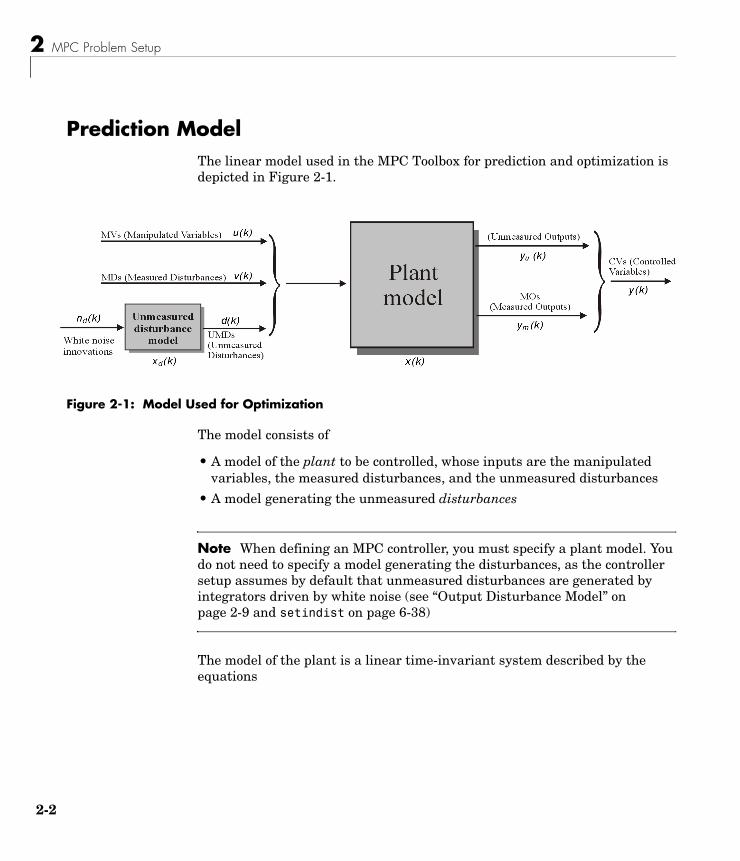
Prediction ModelThe linear model used in the MPC Toolbox for prediction and optimization is depicted in Figure 2-1.
Figure 2-1: Model Used for Optimization
The model consists of
• A model of the plant to be controlled, whose inputs are the manipulated variables, the measured disturbances, and the unmeasured disturbances
• A model generating the unmeasured disturbances
Note When defining an MPC controller, you must specify a plant model. You do not need to specify a model generating the disturbances, as the controller setup assumes by default that unmeasured disturbances are generated by integrators driven by white noise (see “Output Disturbance Model” on page 2-9 and setindist on page 6-38)
The model of the plant is a linear time-invariant system described by the equations

Prediction Model
where x(k) is the nx-dimensional state vector of the plant, u(k) is the nu-dimensional vector of manipulated variables (MV), i.e., the command inputs, v(k) is the nv-dimensional vector of measured disturbances (MD), d(k) is the nd-dimensional vector of unmeasured disturbances (UD) entering the plant, ym(k) is the vector of measured outputs (MO), and yu(k) is the vector of unmeasured outputs (UO). The overall output vector y(k) collects ym(k) and yu(k).
The Model Predictive Control Toolbox accepts both plant models specified as LTI objects, and models obtained from input/output data using the System Identification Toolbox (IDMODEL objects), see Using Identified Models (p. 2-19).
In the above equations d(k) collects both state disturbances (Bd≠0) and output disturbances (Dd≠0).
Note A valid plant model for the MPC Toolbox cannot have direct feedthrough of manipulated variables u(k) on the measured output vector ym(k).
The unmeasured disturbance d(k) is modeled as the output of the linear time invariant system
(2-1)
. (2-2)
The system described by the above equations is driven by the random Gaussian noise nd(k), having zero mean and unit covariance matrix. For instance, a step-like unmeasured disturbance is modeled as the output of an integrator. Input disturbance models as in the equations above can be manipulated by using the methods getindist on page 6-14 and setindist on page 6-38.
x k 1+( ) Ax k( ) Buu k( ) Bvv k( ) Bdd k( )+ + +=
ym k( ) Cmx k( ) Dvmv k( ) Ddmd k( )+ +=
yu k( ) Cux k( ) Dvuv k( ) Ddud k( ) Duuu k( )+ + +=
xd k 1+( ) Axd k( ) Bnd k( )+=
d k( ) Cxd k( ) Dnd k( )+=
2-3

2 MPC Problem Setup
2-4
Note If continuous-time models are supplied, they are internally sampled with the controller’s sampling time.
OffsetsIn many practical applications, the matrices A, B, C, D of the model representing the process to control are obtained by linearizing a nonlinear dynamical system, such as
,
at some nominal value x=x0, u=u0, v=v0, d=d0. In these equations x′ denotes either the time derivative (continuous time model) or the successor x(k+1) (discrete time model). As an example, x0, u0, v0, d0 may be obtained by using TRIM on a simulink model describing the nonlinear dynamical equations, and A, B, C, D by using LINMOD. The linearized model has the form
The matrices A, B, C, D of the model are readily obtained from the Jacobian matrices appearing in the equations above.
The linearized dynamics are affected by the constant terms F=f(x0, u0, v0, d0) and H=h(x0, u0, v0, d0). For this reason the MPC algorithm internally adds a measured disturbance v=1, so that F and H can be embedded into Bv and Dv, respectively, as additional columns.
Note Nonzero offset values d0 for unmeasured disturbances, while relevant for obtaining the linearized model matrices, are not relevant for the MPC problem setup. In fact, only d-d0 can be estimated from output measurements.
x' f x u v d, , ,( )=
y h x u v d, , ,( )=
x' f x0 u0 v0 d0, , ,( ) ∇xf x0 u0 v0 d0, , ,( ) x x0–( ) ∇uf x0 u0 v0 d0, , ,( ) u u0–( )∇vf x0 u0 v0 d0, , ,( ) v v0–( ) ∇df x0 u0 v0 d0, , ,( ) d d0–( )+
+ ++
≅
y h x0 u0 v0 d0, , ,( ) ∇xh x0 u0 v0 d0, , ,( ) x x0–( ) ∇uh x0 u0 v0 d0, , ,( ) u u0–( )∇vh x0 u0 v0 d0, , ,( ) v v0–( ) ∇dh x0 u0 v0 d0, , ,( ) d d0–( )+
+ ++
≅

Optimization Problem
2
1–
Optimization ProblemAssume that the estimates of x(k), xd(k) are available at time k (for state estimation see “State Estimation” on page 2-8). The MPC control action at time k is obtained by solving the optimization problem
(2-3)
where the subscript “( )j” denotes the j-th component of a vector, “(k+i|k)” denotes the value predicted for time k+i based on the information available at time k; r(k) is the current sample of the output reference, subject to
(2-4)
with respect to the sequence of input increments {∆u(k|k),…,∆u(m-1+k|k)} and to the slack variable ε, and by setting u(k)=u(k-1)+∆u(k|k)*, where ∆u(k|k)* is the first element of the optimal sequence.
Note Although only the measured output vector ym(k) is fed back to the MPC controller, r(k) is a reference for all the outputs (measured and unmeasured).
When the reference r is not known in advance, the current reference r(k) is used over the whole prediction horizon, namely r(k+i+1)=r(k) in Equation 2-3. In model predictive control the exploitation of future references is referred to as anticipative action (or look-ahead or preview). A similar anticipative action can
min∆u k k( ) … ∆u m 1– k k+( ) ε,, ,
wi 1 j,+y yj k i 1 k+ +( ) rj k i 1+ +( )–( )
wi j,∆u∆uj k i k+( )
2wi j,
u uj k i k+( ) ujtarget k i+( )–( )2
j 1=
nu
∑+
j 1=
nu
∑+
j 1=
ny
∑⎝
⎠
⎜
⎟
⎜
⎟
⎛
⎞ρεε2+
i 0=
p 1–
∑⎩
⎭
⎪
⎪
⎨
⎬
⎪
⎪
⎧
⎫
ujmin i( ) εVju
min i( )– uj k i k+( ) ujmax i( ) εVju
max i( )+≤ ≤
∆ujmin i( ) εVj∆u
min i( )– ∆uj k i k+( ) ∆ujmax i( ) εVj∆u
max i( )+≤ ≤
yjmin i( ) εVjymin i( )– yj k i 1+ k+( ) yjmax i( ) εVj
ymax i( )+≤ ≤
∆u k h k+( ) 0 h m … p 1–, ,=,=ε 0≥
i 0 … p, ,=
2-5

2 MPC Problem Setup
2-6
be performed with respect to measured disturbances v(k), namely v(k+i)=v(k) if the measured disturbance is not known in advance (e.g. is coming from a Simulink block) or v(k+i) is obtained from the workspace. In the prediction, d(k+i) is instead obtained by setting nd(k+i)=0 in Figure 2-1 and Figure 2-2.
w∆ui,j, w
ui,j, w
yi,j, are nonnegative weights for the corresponding variable. The
smaller w, the less important is the behavior of the corresponding variable to the overall performance index.
uj,min, uj,max, ∆uj,min, ∆uj,max, yj,min, yj,max are lower/upper bounds on the corresponding variables. In Equation 2-4, the constraints on u, ∆u, and y are relaxed by introducing the slack variable ε≥ 0. The weight ρε on the slack variable ε penalizes the violation of the constraints. The larger ρε with respect to input and output weights, the more the constraint violation is penalized. The Equal Concern for the Relaxation (ECR) vectors Vu
min,Vumax, V∆u
min, VDumax,
Vymin, Vy
max have nonnegative entries which represent the concern for relaxing the corresponding constraint; the larger V, the softer the constraint. V=0 means that the constraint is a hard one that cannot be violated. By default, all input constraints are hard (Vu
min=Vumax=V∆u
min=V∆umax=0) and
all output constraints are soft (Vymin=Vy
max=1). As hard output constraints may cause infeasibility of the optimization problem (for instance, because of unpredicted disturbances, model mismatch, or just because of numerical round off), a warning message is produced if Vy
min, Vymax are smaller than a given
small value and automatically adjusted at that value. By default,
(2-5)
Note that also ECRs can be time varying.
Vector utarget(k+i) is a setpoint for the input vector. One typically uses utarget if the number of inputs is greater than the number of outputs, as a sort of lower-priority setpoint.
As mentioned earlier, only ∆u(k|k) is actually used to compute u(k). The remaining samples ∆ u(k+i|k) are discarded, and a new optimization problem based on ym(k+1) is solved at the next sampling step k+1.
The algorithm implemented in the Toolbox uses different procedures depending on the presence of constraints. If all the bounds are infinite, then the slack variable ε is removed, and the problem in Equation 2-3 and Equation 2-4 is solved analytically. Otherwise a Quadratic Programming (QP) solver is used.
ρε 105max wi j,∆u w, i j,
uwi j,
y,⎩ ⎭⎨ ⎬⎧ ⎫
=
Optimization Problem
The matrices associated with the quadratic optimization problem are described in “QP Matrices” on page 2-12.
Since output constraints are always soft, the QP problem is never infeasible. If for numerical reasons the QP problem becomes infeasible, the second sample from the previous optimal sequence is applied, i.e. u(k)=u(k-1)+∆*u(k|k-1).
Note For reasons of numerical robustness, for constrained MPC problems the default value ∆uj,min for unbounded input rates is -10 and the maximum allowed lower bound is -1e5. The default value for unconstrained problems is minus infinity.
2-7

2 MPC Problem Setup
2-8
State EstimationAs the states x(k), xd(k) are not directly measurable, predictions are obtained from a state estimator. In order to provide more flexibility, the estimator is based on the model depicted in Figure 2-2.
Figure 2-2: Model Used for State Estimation
Measurement Noise ModelWe assume that the measured output vector ym(k) is corrupted by a measurement noise m(k). The measurement noise m(t) is the output of the linear time-invariant system
.
The system described by these equations is driven by the random Gaussian noise nm(k), having zero mean and unit covariance matrix.
xm k 1+( ) Axm k( ) Bnm k( )+=
m k( ) Cxm k( ) Dnm k( )+=

State Estimation
Note The objective of the MPC controller is to bring yu(k) and [ym(k)-m(k)] as close as possible to the reference vector r(k). For this reason, the measurement noise model producing m(k) is not needed in the prediction model used for optimization described in “Prediction Model” on page 2-2.
Output Disturbance ModelIn order to guarantee asymptotic rejection of output disturbances, the overall model is augmented by an output disturbance model. By default, in order to reject constant disturbances due for instance to gain nonlinearities, the output disturbance model is a collection of integrators driven by white noise on measured outputs. Output integrators are added according to the following rule:
1 Measured outputs are ordered by decreasing output weight (in case of time-varying weights, the sum of the absolute values over time is considered for each output channel, and in case of equal output weight the order within the output vector is followed)
2 By following such order, an output integrator is added per measured outputs, unless there is a violation of observability, or the corresponding weight is zero, or the user forces it (through the OutputVariables.Integrators property described in “OutputVariables” on page 8-5).
An arbitrary output disturbance model can be specified through the function setoutdist on page 6-43. See also setoutdist on page 6-43 for ways to remove the default output integrators.
State ObserverThe state observer is designed to provide estimates of x(k), xd(k), xm(k), where x(k) is the sta=ate of the plant model, xd(k) is the overall state of the input and output disturbance model, xm(k) is the state of the measurement noise model. The estimates are computed from the measured output ym(k) by the linear state observer
2-9

2 MPC Problem Setup
2-1
d k( )
m k( )
u k( )
v k( )
where “m” denotes the rows of C,D corresponding to measured outputs.
To prevent numerical difficulties in the absence of unmeasured disturbances, the gain M is designed using Kalman filtering techniques (see the function KALMAN in the Control System Toolbox) on the extended model
(2-6)
where nu(k) and nv(k) are additional unmeasured white noise disturbances having unit covariance matrix and zero mean, that are added on the vector of manipulated variables and the vector of measured disturbances, respectively, to ease the solvability of the Kalman filter design.
x k k( )xd k k( )
xm k k( )
x k k 1–( )xd k k 1–( )
xm k k 1–( )
M ym k( ) ym k( )–( )+=
x k 1+ k( )xd k 1+ k( )
xm k 1+ k( )
Ax k k( ) Buu k( ) Bvv k( ) BdCxd k k( )+ + +
Axd k k( )
Axm k k( )
=
ym k( ) Cmx k k 1–( ) Dvmv k( ) DdmCxd k k 1–( ) Cxm k k 1–( )+ + +=
x k 1+( )xd k 1+( )
xm k 1+( )
A BdC 0
0 A 0
0 0 A
x k( )xd k( )
xm k( )
Bu
00
u k( )Bv
00
v k( )BdD 0 Bu Bv
B 0 0 0
0 B 0 0
n
n
n
n
+ + +=
ym k( ) Cm DdmC C
x k( )xd k( )
xm k( )
Dvmv k( ) Dm D 0 0
nd k( )
nm k( )
nu k( )
nv k( )
+ +=
0

State Estimation
Note The overall state-space realization of the combination of plant and disturbance models must be observable for the state estimation design to succeed. The MPC Toolbox first checks for observability of the plant, provided that this is given in state-space form. After all models have been converted to discrete-time, delay-free, state-space form and combined together, observability of the overall extended model is checked (see the note on page 6-37 and “Construction and Initialization” on page 8-12).
Note also that observability is only checked numerically. Hence, for large models of badly conditioned system matrices, unobservability may be reported by the MPC Toolbox even if the system is observable.
See also getestim on page 6-11 and setestim on page 6-36 for details on the methods that you can use to access and modify properties of the state estimator.
2-11

2 MPC Problem Setup
2-1
QP Matrices This section describes the matrices associated with the MPC optimization problem described in “Optimization Problem” on page 2-5.
PredictionAssume for simplicity that the disturbance model in Equation 2-1 and Equation 2-2 is a unit gain (i.e., d(k)=nd(k) is a white Gaussian noise). For simplicity, denote by
Then, the prediction model given by
.
Consider for simplicity the prediction of the future trajectories of the model performed at time k=0. We set nd(i)=0 for all prediction instants i, and obtain
which gives
where
x xxd
A A BdC
0 ABu
Bu
0Bv
Bv
0Bd
BdD
BC C DdC←,←,←,←,←,←
x k 1+( ) Ax k( ) Buu k( ) Bvv k( ) Bdnd k( )+ + +=
y k( ) Cx k( ) Dvv k( ) Ddnd k( )+ +=
y i 0( ) C Aix 0( ) Ai 1– Bu u 1–( ) ∆u j( )
j 0=
h
∑+⎝ ⎠⎜ ⎟⎜ ⎟⎛ ⎞
Bvv h( )+⎝ ⎠⎜ ⎟⎜ ⎟⎛ ⎞
h 0=
i 1–
∑+ Dvv i( )+=
y 1( )…
y p( )
Sxx 0( ) Su1u 1–( ) Su
∆u 0( )…
∆u p 1–( )
Hv
v 0( )…
v p( )
+ + +=
2

QP Matrices
Optimization VariablesLet m be the number of free control moves and denote by z= [z0; ...; zm-1]. Then,
(2-7)
where JM depends on the choice of blocking moves. Together with the slack variable ε, vectors z0, ..., zm-1 constitute the free optimization variables of the optimization problem (in case of systems with a single manipulated variables, z0, ..., zm-1 are scalars).
Sx
CA
CA2
…
CAp
ℜpny nx×
∈ Su1,
CBu
CBu CABu+
…
CAhBu
h 0=
p 1–
∑
ℜpny nu×
∈= =
Su
CBu 0 … 0
CBu CABu+ CBu … 0
… … … …
CAhBu
h 0=
p 1–
∑ CAhBu
h 0=
p 2–
∑ … CBu
ℜpny pnu×
∈=
Hv
CBv Dv 0 … 0
CABv CBv Dv … 0
… … … … …
CAp 1– Bv CAp 2– Bv CAp 3– Bv … Dv
ℜpny p 1+( )nv×
∈=
∆u 0( )…
∆u p 1–( )
JM
z0
…zm 1–
=
2-13

2 MPC Problem Setup
2-1
Figure 2-3: Blocking Moves: Inputs and Input Iincrements for moves=[2 3 2]
Consider for instance the blocking moves depicted in Figure 2-3, which corresponds to the choice moves=[2 3 2], or, equivalently, u(0)=u(1), u(2)=u(3)=u(4), u(5)=u(6), ∆ u(0)=z0, ∆ u(2)=z1, ∆ u(5)=z2, ∆ u(1)=∆ u(3)=∆ u(4)=∆ u(6)=0.
Then, the corresponding matrix JM is
JM
I 0 00 0 00 I 00 0 00 0 00 0 I0 0 0
=
4

QP Matrices
Cost FunctionThe function to be optimized is
where
Finally, after substituting u(k), ∆u(k), y(k), J(z) can be rewritten as
(2-8)
J z ε,( )u 0( )
…u p 1–( )
utarget 0( )
…utarget p 1–( )
–
⎝ ⎠⎜ ⎟⎜ ⎟⎜ ⎟⎛ ⎞T
W2u
u 0( )…
u p 1–( )
utarget 0( )
…utarget p 1–( )
–
⎝ ⎠⎜ ⎟⎜ ⎟⎜ ⎟⎛ ⎞
∆u 0( )…
∆u p 1–( )
T
W2∆u
∆u 0( )…
∆u p 1–( )
y 1( )…
y 1( )
r 1( )…
r p( )
–
⎝ ⎠⎜ ⎟⎜ ⎟⎜ ⎟⎛ ⎞T
W2y
y 1( )…
y 1( )
r 1( )…
r p( )
–
⎝ ⎠⎜ ⎟⎜ ⎟⎜ ⎟⎛ ⎞
ρεε2
+
+
+ +
=
Wu diag w0 1,u w0 2,
u … w0 nu,u … wp 1– 1,
u w0p 1– 2,u … wp 1– nu,
u, , , , , , , ,( )=
W∆u diag w0 1,∆u w0 2,
∆u … w0 nu,∆u … wp 1– 1,
∆u w0p 1– 2,∆u … wp 1– nu,
∆u, , , , , , , ,( )=
Wy diag w1 1,y w1 2,
y … w1 ny,y … wp 1,
y wp 2,y … wp ny,
y, , , , , , , ,( )=
J z ε,( ) ρεε2 zTK∆uz 2r 1( )…
r p( )
T
Kr
v 0( )…
v p( )
Kv u 1–( )TKu
utarget 0( )
…utarget p 1–( )
T
Kut x 0( )TKx
+ +
+ +
⎝
⎠
⎜
⎟
⎜
⎟
⎜
⎟
⎛
⎞
z constant
+ +
+
=
2-15

2 MPC Problem Setup
2-1
1)
)
1– )
Note In order to keep the QP problem always strictly convex, if the condition number of the Hessian matrix K∆U is larger than 1012, the quantity 10*sqrt(eps) is added on each diagonal term. This may only occur when all input rates are not weighted (W∆u=0) (see note on page 8-8)
ConstraintsLet us now consider the limits on inputs, input increments, and outputs along with the constraint ε≥ 0
Note Upper and lower bounds that are not finite are removed, as well as the input and input-increment bounds over blocked moves.
Similarly to what was done for the cost function, we can substitute u(k), ∆u(k), y(k), and obtain
(2-9)
ymin 1( ) εVymin 1( )–
…
ymin p( ) εVymin p( )–
umin 0( ) εVumin 0( )–
…
umin p 1–( ) εVumin p 1–( )–
∆umin 0( ) εV∆umin 0( )–
…
∆umin p 1–( ) εV∆umin p 1–( )–
y 1( )…
y p( )u 0( )
…u p 1–( )∆u 0( )
…∆u p 1–( )
ymax 1( ) εVymax 1( )+
…
ymax p( ) εVymax p( )+
umax 0( ) εVumax 0( )+
…
umax p 1–( ) εVumax p –(+
∆umax 0( ) εV∆umax 0(+
…
∆umax p 1–( ) εV∆umax p(+
≤ ≤
Mzz Mεε Mlim Mv
v 0( )…
v p( )
Muu 1–( ) Mxx 0( )+ + +≤+
6

QP Matrices
where matrices Mz,Mε,Mlim,Mv,Mu,Mx are obtained from the upper and lower bounds and ECR values.
The matrices of the QP problem are built in function mpc_buildmat.
2-17
2 MPC Problem Setup
2-1
x
⎠⎟⎟⎟⎞T
MPC ComputationThis section describes how the MPC optimization problem is solved at each time step k (in mpcmove, mpc_sfun.dll, and mpcloop_engine.dll) by using the matrices built at initialization described in “QP Matrices” on page 2-12.
Unconstrained MPCThe optimal solution is computed analytically:
and the MPC controller sets ∆u(k)=z*0, u(k)=u(k-1)+∆u(k).
Constrained MPCThe optimal solution z*, ε* is computed by solving the quadratic program
described in Equation 2-8 and Equation 2-9, using the QP solver coded in the
qpsolver.dll function (see qpdantz on page 6-33 for more details).
z∗ K 1–∆u
r 1( )…
r p( )
T
Kr
v 0( )…
v p( )
Kv u 1–( )TKu
utarget 0( )
…utarget p 1–( )
T
Kut x 0( )TK+ + + +
⎝⎜⎜⎜⎛
–=
8

Using Identified Models
Using Identified ModelsThe MPC Toolbox is able to handle plant models generated by the System Identification Toolbox from input/output measurements.
The MPC Toolbox labels control input signals as ‘Manipulated’, measured input disturbances as ‘Measured’, and unmeasured input disturbances as ‘Unmeasured’. On the other hand, the System Identification Toolbox has a different naming rule, as it calls ‘Measured’ the inputs that are measurable quantities, and ‘Noise’ those that are not.
When you specify an identified model in the MPC constructor as the plant model, the MPC Toolbox treats ‘Noise’ signals as ‘Unmeasured’ input signals, and ‘Measured’ signals as ‘Manipulated’ signals, assuming that all measured inputs are also manipulated variables. You can later change later signal types, for instance to specify that some measured inputs are measured disturbances, rather than manipulated variables (See setname on page 6-42).
The MPC Toolbox internally converts the identified model you have provided as a plant model into the classical (A,B,C,D) state-space format. The columns of the B matrix originally related to ‘Noise’ channels are treated as the effect of unmeasured input disturbances on the state of the plant. On the other hand, the columns of the D matrix related to ‘Noise’ channels as treated as the effect of measurement noise superimposed on the output signal. Accordingly, the MPC Toolbox treats as the plant model the state-space model obtained from (A,B,C,D) by zeroing the columns of D related to ‘Noise’ channels. Those columns are instead used as a static noise model, or cascaded to an existing noise model if you have specified one. A unit static gain is assumed as the disturbance model, unless you have specified another one.
2-19

2 MPC Problem Setup
2-2
0
3
MPC Simulink LibraryMPC Controller Block (p. 3-2) A discussion of the Simulink block representing an MPC controller as defined by an MPC object.

3 MPC Simulink Library
3-2
MPC Controller Block
Opening the LibraryThe MPC Simulink Library provides a single block representing the MPC controller.
The library can be opened from the main Simulink library or by typing mpclib from the command prompt.
Figure 3-1: MPC Simulink Library
After copying the MPC Controller block in your diagram, you can double-click on the block and open the mask window.
MPC Controller Block
MPC Controller Block Mask
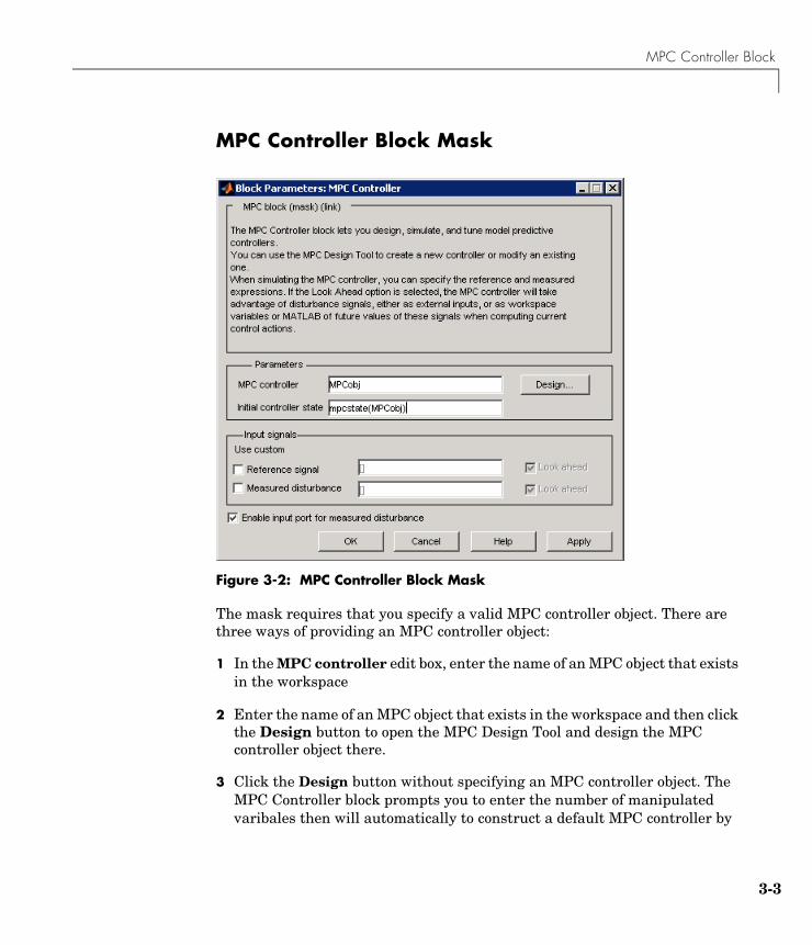
Figure 3-2: MPC Controller Block Mask
The mask requires that you specify a valid MPC controller object. There are three ways of providing an MPC controller object:
1 In the MPC controller edit box, enter the name of an MPC object that exists in the workspace
2 Enter the name of an MPC object that exists in the workspace and then click the Design button to open the MPC Design Tool and design the MPC controller object there.
3 Click the Design button without specifying an MPC controller object. The MPC Controller block prompts you to enter the number of manipulated varibales then will automatically to construct a default MPC controller by
3-3

3 MPC Simulink Library
3-4
linearizing the plant model from the Simulink diagram. This option requires Simulink Control Design. See “Importing a Plant Model” on page 5-9 for more information about creating linearized plant models with the MPC Toolbox. Refer to the Simulink Control Design documentation for more information about the linearization process.
Note Closed-loop simulations can be run while the MPC controller is edited in the MPC Design Tool. In this case, the controller parameters used for simulating the Simulink diagram are those currently specified in the MPC Design Tool, so that the parameters of the controller can be more easily tuned. Once the MPC Design Tool is closed, the designed controller must be exported as an MPC object to the workspace in order to be used in simulation.
Look Ahead and Signals from the WorkspaceReference and measured disturbance signals, by default, are taken from the Simulink diagram. They can be taken instead from the workspace. In this case, store the signal in a structure having the same format as used in the Simulink From Workspace and To Workspace blocks. This requires two fields: time and signals.
For example, to specify the sinusoidal reference signal sin(t) over a time horizon of 10 seconds, assuming an MPC controller’s sampling time Ts, use
time=(0:Ts:10);ref.time=time;ref.signals.values=sin(time);
An alternative would be to run a separate Simulink simulation to create the stored signal. Use the blocks required to define the signal (e.g., Sine in the above example), and store the result using a To Workspace block.
The Look ahead check box enables an anticipative action on the corresponding signal. It can only be enabled if the signal comes from the workspace.
See the demo mpcpreview for an illustrative example of enabling preview and reading signals from the workspace.

MPC Controller Block
InitializationThe initial controller state must be a valid mpcstate object. See “MPC State Object” on page 8-13.
Using the MPC Toolbox with Real-Time Workshop®The C sources of the S-function executing the MPC Controller Block code are available in the mpcutils/src directory. You can build a real-time executable by pressing Ctrl+B on your Simulink diagram to invoke Real-Time Workshop and build the model.
In some cases, it is necessary to copy the source files (mpc_sfun.c, mpc_sfun.h, mpc_common.c, mat_macros.h, dantzgmp.h, dantzgmp_solver.c) to a visible directory, such as the current directory '.', or 'C:\MATLAB\rtw\c\src'.
The MPC Controller Block can be also used to produce real-time executables that run under xPC Target.
3-5

3 MPC Simulink Library
3-6

4
Case-Study Examples
This chapter describes some typical MPC applications. Familiarity with LTI models (from the Control System Toolbox) and Simulink block diagrams will make the examples easier to understand, but you can skip the modeling details if you wish.
The first example designs a servomechanism controller. The specifications require a fast servo response despite constraints on a plant input and a plant output.
The second example controls a paper machine headbox. The process is nonlinear, and has three outputs, two manipulated inputs, and two disturbance inputs, one of which is measured for feedforward control.
Servomechanism Controller (p. 4-2) MPC Toolbox design of a servomechanism. Uses MPCTOOL GUI and commands.
Paper Machine Process Control (p. 4-30)
Application to a paper machine headbox. Involves multiple signals. Illustrates use of MPCTOOL GUI and Simulink.

4 Case-Study Examples
4-2
Servomechanism Controller
Figure 4-1: Position Servomechanism Schematic
System ModelA position servomechanism consists of a DC motor, gearbox, elastic shaft, and a load (see Figure 4-1). The differential equations representing this system are
where V is the applied voltage, T is the torque acting on the load, is the load’s angular velocity, is the motor shaft’s angular velocity, and the other symbols represent constant parameters (see Table 4-1 for more information on these).
If we define the state variables as , we can convert the above model to an LTI state-space form:
ω· LkθJL------- θL
θMρ
-------–⎝ ⎠⎛ ⎞–
βLJL-------ωL–=
ω· MkTJM--------
V kTωM–R
--------------------------⎝ ⎠⎛ ⎞ βMωM
JM-----------------–
kθρJM------------ θL
θMρ
-------–⎝ ⎠⎛ ⎞+=
ωL θ· L=ωM θ· M=
xp θL ωL θM ωM
T=

Servomechanism Controller
Table 4-1: Parameters Used in the Servomechanism Model
Symbol Value (SI units)
Definition
1280.2 Torsional rigidity
10 Motor constant
0.5 Motor inertia
50 Nominal load inertia
20 Gear ratio
0.1 Motor viscous friction coefficient
25 Load viscous friction coefficient
R 20 Armature resistance
x·p
0 1 0 0kθJL-------–
βLJL-------–
kθρJL---------- 0
0 0 0 1
kθρJM------------ 0
kθ
ρ2JM
--------------–βM kT
2 R⁄+JM
-----------------------------–
xp
000
kTRJM-------------
V+=
θL 1 0 0 0 xp=
T kθ 0kθρ------– 0 xp=
kθ
kT
JM
JL JM
ρ
βM
βL
4-3

4 Case-Study Examples
4-4
Control Objectives and ConstraintsThe controller must set the load’s angular position, , at a desired value by adjusting the applied voltage, V. The only measurement available for feedback is .
The elastic shaft has a finite shear strength, so the torque, T, must stay within specified limits
N m
Also, the applied voltage must stay within the range
V
From an input/output viewpoint, the plant has a single input, V, which is manipulated by the controller. It has two outputs, one measured and fed back to the controller, , and one unmeasured, T.
Defining the Plant ModelThe first step in a design is to define the plant model. The following commands are from the mpcdemos file motor_model.m, which you can run instead of entering the commands manually.
% DC-motor with elastic shaft%%Parameters (MKS)%------------------------------------------------------------------------------------------Lshaft=1.0; %Shaft lengthdshaft=0.02; %Shaft diametershaftrho=7850; %Shaft specific weight (Carbon steel)G=81500*1e6; %Modulus of rigiditytauam=50*1e6; %Shear strengthMmotor=100; %Rotor massRmotor=.1; %Rotor radiusJmotor=.5*Mmotor*Rmotor^2; %Rotor axial moment of inertia Bmotor=0.1; %Rotor viscous friction coefficient (A CASO)R=20; %Resistance of armatureKt=10; %Motor constant
θL
θL
T 78.5≤
V 220≤
θL

Servomechanism Controller
gear=20; %Gear ratioJload=50*Jmotor; %Load NOMINAL moment of inertiaBload=25; %Load NOMINAL viscous friction coefficientIp=pi/32*dshaft^4; %Polar momentum of shaft (circular) sectionKth=G*Ip/Lshaft; %Torsional rigidity (Torque/angle)Vshaft=pi*(dshaft^2)/4*Lshaft; %Shaft volumeMshaft=shaftrho*Vshaft; %Shaft massJshaft=Mshaft*.5*(dshaft^2/4); %Shaft moment of inertiaJM=Jmotor; JL=Jload+Jshaft;Vmax=tauam*pi*dshaft^3/16; %Maximum admissible torqueVmin=-Vmax;
%Input/State/Output continuous time form%------------------------------------------------------------------------------------------AA=[0 1 0 0; -Kth/JL -Bload/JL Kth/(gear*JL) 0; 0 0 0 1; Kth/(JM*gear) 0 -Kth/(JM*gear^2) -(Bmotor+Kt^2/R)/JM]; BB=[0;0;0;Kt/(R*JM)];Hyd=[1 0 0 0];Hvd=[Kth 0 -Kth/gear 0];Dyd=0;Dvd=0;
% Define the LTI state-space modelsys=ss(AA,BB,[Hyd;Hvd],[Dyd;Dvd]);
Controller Design Using MPCTOOLThe servomechanism model is linear, so you can use the MPC Toolbox design tool (mpctool) to configure a controller and test it.
4-5

4 Case-Study Examples
4-6
Note To follow this example on your own system, first create the servomechanism model as explained above. This defines the variable sys in your MATLAB workspace.
Opening MPCTOOL and Importing a ModelTo begin, open the design tool by typing the following at the MATLAB prompt:
mpctool
Once the design tool has appeared, click the Import Plant button. The Plant Model Importer will appear (see Figure 4-2).
By default, the Import from radio buttons are set to import from the MATLAB workspace, and the box at the upper right lists all LTI models defined there. In Figure 4-2, sys is the only available model, and it is selected. The Properties window lists the selected model’s key attributes.

Servomechanism Controller
Figure 4-2: Import Dialog with the Servomechanism Model Selected
Make sure your servomechanism model, sys, is selected. Then click the Import button. Your model loads, and tables appear in the design tool’s main window (see Figure 4-3). The diagram at the top shows the number of inputs and outputs in your model.
Specifying Signal PropertiesIt’s essential to specify signal types before going on. By default, the design tool assumes all plant inputs are manipulated, which is correct in this case. But it also assumes all outputs are measured, which is not. Specify that the second output is unmeasured by clicking on the appropriate table cell and selecting the Unmeasured option.
4-7

4 Case-Study Examples
4-8
Figure 4-3: Design Tool After Importing the Plant Model and Specifying Signal Properties
You also have the option to change the default signal names (In1, Out1, Out2) to something more meaningful (e.g., V, ThetaL, T), enter descriptive information in the blank Description and Units columns, and specify a nominal initial value for each signal (the default is zero).

Servomechanism Controller
After you’ve entered all your changes, you should see a view similar to Figure 4-3. Notice that the graphic shows the effect of designating one output as measured, the other unmeasured.
Navigation Using the Tree ViewNow consider the design tool’s left-hand frame. This tree is an ordered arrangement of nodes. By default, the root node is named MPCdesign, and is selected when the design tool starts. Whenever you select the root node, the starting view shown in Figure 4-3 reappears.
The Plant models node is next in the hierarchy. Click on it to list the plant models being used in your design. (Each model name is editable.) The middle section displays the selected model’s properties. There is also a space to enter notes describing the model’s special features. Buttons allow you to import a new model or delete one you no longer need.
The next node is Controllers. You might see a + sign to its left, indicating that it contains subnodes. If so, click on the + sign to expand the tree (as shown in Figure 4-3). All the controllers in your design will appear here. By default, you have one: MPC1. In general, you might opt to design and test several alternatives.
Select Controllers to see a list of all controllers, similar to the Plant models view. The table columns show important controller settings: the plant model being used, the controller sampling period, and the prediction and control horizons. All are editable. For now, leave them at their default values.
The buttons on the Controllers view allow you to:
• Import a controller designed previously and stored either in your workspace or in a MAT-file
• Export the selected controller to your workspace
• Create a New controller, which will be initialized to the MPC Toolbox defaults
• Copy the selected controller to create a duplicate that you can modify
• Delete the selected controller
4-9

4 Case-Study Examples
4-1
Specifying Controller PropertiesSelect the MPC1 subnode. The main panel should change to the MPC design view shown in Figure 4-4.
Figure 4-4: Controller Design View, Models and Horizons Pane
If the selected Prediction model is continuous-time, as in this example, the Control interval (sampling period) defaults to 1. You need to change this to an
0

Servomechanism Controller
application-appropriate value. Set it to 0.1 seconds (as shown in Figure 4-4). Leave the other values at their defaults for now..
Figure 4-5: Controller Design View, Constraints Pane
4-11

4 Case-Study Examples
4-1
Specifying ConstraintsNext, select the Constraints tab. The view shown in Figure 4-5 appears. Enter the appropriate constraint values. Leaving a field blank implies that there is no constraint.
In general, it’s good practice to include all known manipulated variable constraints, but it’s unwise to enter constraints on outputs unless they are an essential aspect of your application. The limit on applied torque is such a constraint, as are the limits on applied voltage. The angular position has physical limits, the controller shouldn’t attempt to enforce them, so you should leave the corresponding fields blank (see Figure 4-5)
The Max down rate should be nonpositive (or blank). It limits the amount a manipulated variable can decrease in a single control interval. Similarly, the Max up rate should be nonnegative. It limits the increasing rate. Leave both unconstrained (i.e., blank).
The shaded columns can’t be edited. If you want to change this descriptive information, select the root node view and edit its tables. (Such changes apply to all controllers in the design.)
Weight TuningNext, select the Weight Tuning tab to obtain a view like that shown in Figure 4-6.
The weights specify trade-offs in the controller design. First consider the Output weights. The controller will try to minimize the deviation of each output from its setpoint or reference value. For each sampling instant in the prediction horizon, the controller multiplies predicted deviations for each output by the output’s weight, squares the result, and sums over all sampling instants and all outputs. One of the controller’s objectives is to minimize this sum, i.e., to provide good setpoint tracking (See “Optimization Problem” on page 2-5 for more details.)
Here, the angular position should track its setpoint, but the applied torque can vary, provided that it stays within the specified constraints. Therefore, set the torque’s weight to zero, which tells the controller that setpoint tracking is unnecessary for this output.
Similarly, it’s acceptable for the applied voltage to deviate from nominal (it must in order to change the angular position!). Its weight should be zero (the default for manipulated variables). On the other hand, it’s probably
2

Servomechanism Controller
undesirable for the controller to make drastic changes in the applied voltage. The Rate weight penalizes such changes. Use the default, 0.1.
When setting the rates, the relative magnitudes are more important than the absolute values, and you must account for differences in the measurement scales of each variable. For example, if a deviation of 0.1 units in variable A is just as important as a deviation of 100 units in variable B, variable A’s weight must be 1000 times larger than that for variable B.
Figure 4-6: Controller Design View, Weight Tuning Pane
The tables allow you to weight individual variables. The slider at the top adjusts an overall trade-off between controller action and setpoint tracking. Moving the slider to the left places a larger overall penalty on manipulated
4-13

4 Case-Study Examples
4-1
variable changes. This usually increases controller robustness, but setpoint tracking becomes more sluggish.
The Estimation tab allows you to adjust the controller’s response to unmeasured disturbances (not used in this example)..
Figure 4-7: Simulation Settings View for “Scenario1”
4

Servomechanism Controller
Defining a Simulation ScenarioIf you haven’t already done so, expand the Scenarios node to show the Scenario1 subnode (see Figure 4-3). Select Scenario1 to obtain the view shown in Figure 4-7.
A scenario is a set of simulation conditions. As shown in Figure 4-7, you choose the controller to be used (from among controllers in your design), the model to act as the plant, and the simulation duration.
You must also specify all setpoints and disturbance inputs.
Duplicate the settings shown in Figure 4-7, which will test the controller’s servo response to a unit-step change in the angular position setpoint. All other inputs are being held constant at their nominal values.
Note The ThetaL and V unmeasured disturbances allow you to simulate additive disturbances to these variables. By default, these disturbances are turned off, i.e., zero.
The Look ahead option designates that all future setpoint variations are known. In that case, the controller can adjust the manipulated variable(s) in advance to improve setpoint tracking. This would be unusual in practice, and is not being used here.
4-15

4 Case-Study Examples
4-1
.
Figure 4-8: Response to Unit Step in the Angular Position Setpoint
Running a SimulationOnce you’re ready to run the scenario, click the Simulate button or the green arrow on the tool bar.
Note The green arrow tool is available from any view once you’ve defined at least one scenario. It runs the active scenario, i.e., the one most recently selected or modified.
We obtain the results shown in Figure 4-8. The blue curves are the output signals, and the gray curves are the corresponding setpoints. The response is very sluggish, and hasn’t settled within the 30 second simulation period.
6

Servomechanism Controller
Note The plot shown in Figure 4-8 provides many of the customization features available in the Control System Toolbox ltiview and sisotool displays. Try clicking on a curve to obtain the numerical characteristics of the selected point, or right-clicking in the plot area to obtain a customization menu.
The corresponding applied voltage adjustments appear in a separate window (not shown) and are also very sluggish.
On the positive side, the applied torque stays well within bounds, as does the applied voltage.
Retuning to Achieve a Faster Servo ResponseTo obtain a more rapid servo response, navigate to the MPC1 Weight Tuning pane (select the MPC1 node to get the controller design view, then select the Weight Tuning tab) and move the slider all the way to the right. Then click on the green arrow in the tool bar. Your results should now resemble Figure 4-9 and Figure 4-10.
The angular position now settles within 10 seconds following the step. The torque approaches its lower limit, but doesn’t exceed it (see Figure 4-9) and the applied voltage stays within its limits (See Figure 4-10).
4-17

4 Case-Study Examples
4-1
.
Figure 4-9: Faster Servo Response
8

Servomechanism Controller
Figure 4-10: Manipulated Variable Adjustments Corresponding to Figure 4-9
Modifying the ScenarioFinally, increase the step size to π radians (select the Scenario1 node and edit the tabular value).
As shown in Figure 4-11 and Figure 4-12, the servo response is essentially as good as before, and we avoid exceeding the torque constraint at -78.5 Nm, even though the applied voltage is saturated for about 2.5 seconds (see Figure 4-12).
4-19

4 Case-Study Examples
4-2
Figure 4-11: Servo Response for Step Increase of π Radians
0

Servomechanism Controller
Figure 4-12: Voltage Adjustments Corresponding to Figure 4-11.
Saving Your WorkOnce you’re satisfied with a controller’s performance, you can export it to the workspace, for use in a Simulink block diagram or for analysis (or you can save it in a MAT-file).
To export a controller, right-click on its node and select Export from the resulting menu (or select the Controllers node, select the controller in the list, and click the Export button). A dialog like that shown in Figure 4-13 will appear.
The Controller source is the design from which you wish to extract a controller. There’s only one in this example, but in general you could be working on several simultaneously. The Controller to export choice defaults to the controller most recently selected. Again, there’s no choice in this case,
4-21

4 Case-Study Examples
4-2
but there could be in general. The Name to assign edit box allows you to rename the exported controller. (This will not change its in the design tool.)
Figure 4-13: Exporting a Controller to the Workspace
Note When you exit the design tool you will be prompted to save the entire design in a MAT file. This allows you to reload it later using the File/Load menu option or the Load icon on the tool bar.
Using MPC Toolbox CommandsOnce you’ve become familiar with the toolbox, you may find it more convenient to build a controller and run a simulation using commands.
For example, suppose that you’ve already defined the model as discussed in “Defining the Plant Model” on page 4-4. Consider the following command sequence:
ManipulatedVariables = struct('Min', -220, 'Max', 220, 'Units', 'V');OutputVariables(1) = struct('Min', -Inf, 'Max', Inf, 'Units', 'rad');OutputVariables(2) = struct('Min', -78.5, 'Max', 78.5, 'Units', 'Nm');Weights = struct('Input', 0, 'InputRate', 0.05, 'Output', [10 0]);
2

Servomechanism Controller
Model.Plant = sys;Model.Plant.OutputGroup = {[1], 'Measured' ; [2], 'Unmeasured'}; Ts = 0.1;PredictionHorizon = 10;ControlHorizon = 2;
This creates several structure variables. For example, ManipulatedVariables defines the display units and constraints for the applied voltage (the manipulated plant input). Weights defines the tuning weights shown in Figure 4-6 (but the numerical values used here provide better performance). Model designates the plant model (stored in sys, which we defined earlier). The code also sets the Model.Plant.OutputGroup property to designate the second output as unmeasured.
Constructing an MPC ObjectUse the mpc command to construct an MPC object called ServoMPC:
ServoMPC = mpc(Model, Ts, PredictionHorizon, ControlHorizon);
Like the LTI objects used to define linear, time-invariant dynamic models, an MPC object contains a complete definition of a controller.
Setting, Getting, and Displaying Object PropertiesOnce you’ve constructed an MPC object, you can change its properties as you would for other objects. For example, to change the prediction horizon, you could use one of the following commands:
ServoMPC.PredictionHorizon = 12;
or
set(ServoMPC, 'PredictionHorizon', 12);
For a listing of all the object’s properties, you could type
get(ServoMPC)
To access a particular one (e.g., the control horizon), you could type
M = get(ServoMPC, 'ControlHorizon');
or
M = ServoMPC.ControlHorizon;
4-23

4 Case-Study Examples
4-2
You can also set multiple properties simultaneously.
Set the following properties before continuing with this example:
set(ServoMPC, 'Weights', Weights, ...'ManipulatedVariables', ManipulatedVariables, ...'OutputVariables', OutputVariables);
Typing the name of an object without a terminating semicolon generates a formatted display of the object’s properties. You can achieve the same effect using the display command:
display(ServoMPC)
Running a SimulationThe sim command performs a linear simulation. For example, the following code sequence defines constant setpoints for the two outputs, then runs a simulation.
TimeSteps = round(10/Ts);r = [pi 0];[y, t, u] = sim(ServoMPC, TimeSteps, r);
By default, the model used to design the controller (stored in ServoMPC) also represents the plant.
The sim command saves the output and manipulated variable sequences in variables y and u. For example,
subplot(311)plot(t, y(:,1), [0 t(end)], pi*[1 1])title('Angular Position (radians)');subplot(312)plot(t, y(:,2), [0 t(end)], [-78.5 -78.5])title('Torque (nM)')subplot(313)stairs(t, u)title('Applied Voltage (volts)')xlabel('Elapsed Time (seconds)')
produces the custom plot shown in Figure 4-14. The plot includes the angular position’s setpoint. The servo response settles within 5 seconds with no overshoot. It also displays the torque’s lower bound, which activates after about
4

Servomechanism Controller
0.9 second, but isn’t exceeded. The applied voltage saturates between about 0.5 and 2.8 seconds, but the controller performs well despite this.
Figure 4-14: Plotting the Output of the Sim Command
4-25

4 Case-Study Examples
4-2
Using MPC Tools in SimulinkFigure 4-15 is a Simulink block diagram for the servomechanism example. Most of the blocks are from the standard Simulink library. There are two exceptions:
• Servomechanism Model is an LTI System block from the Control System Toolbox library. The LTI model sys (which must exist in the workspace) defines its dynamic behavior. To review how to create this model, see “Defining the Plant Model” on page 4-4.
• MPC Controller is from the MPC Blocks library. Figure 4-16 shows the dialog box obtained by double-clicking on this block. You need to supply an MPC object, and ServoMPC is being used here. It must be in the Workspace before you run a simulation. The Design button opens the design tool, which allows you to create or modify the object. To review how to use commands to create ServoMPC, see “Constructing an MPC Object” on page 4-23.
.
Figure 4-15: Block Diagram for the Servomechanism Example
6

Servomechanism Controller
Figure 4-16: MPC Toolbox Simulink Block Dialog
The key features of the diagram are as follows:
• The MPC Controller output is the plant input. The Voltage Scope block plots it (yellow curve). Minimum and maximum voltage values are shown as magenta and cyan curves.
• The plant output is a vector signal. The first element is the measured angular position. The second is the unmeasured torque. A Demux block separates them. The angular position feeds back to the controller and plots
4-27
4 Case-Study Examples
4-2
on the Angle scope (yellow curve). The torque plots on the Torque scope (with its lower and upper bounds).
• The position setpoint varies sinusoidally with amplitude π radians and frequency 0.4 rad/s. It also appears on the Angle scope (magenta curve).
Figure 4-17 shows the scope displays for a 20-second simulation. The angular position tracks the sinusoidal setpoint variations quite well, despite saturation of the applied voltage. The setpoint variations are more gradual than the step changes used previously, so the torque stays well within its bounds.
8
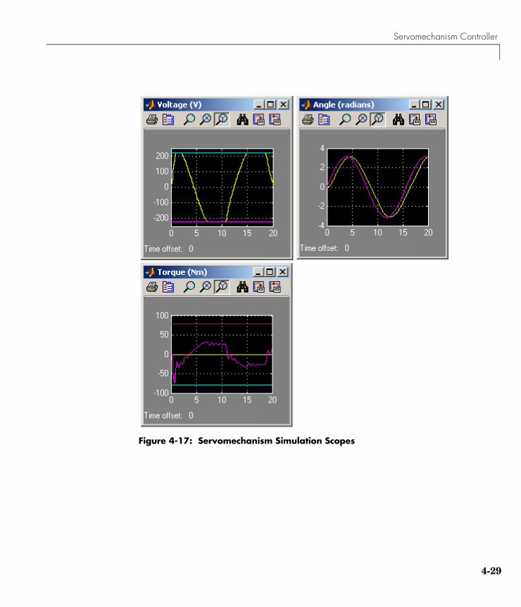
Servomechanism Controller
Figure 4-17: Servomechanism Simulation Scopes
4-29

4 Case-Study Examples
4-3
Paper Machine Process Control
Figure 4-18: Schematic of Paper Machine Headbox Elements
Ying et al. [1] studied the control of consistency (percentage pulp fibers in aqueous suspension) and liquid level in a paper machine headbox, a schematic of which is shown in Figure 4-18. The process model is a set of ordinary differential equations (ODEs) in bilinear form. The states are
where H1 is the liquid level in the feed tank, H2 is the headbox liquid level, N1 is the feed tank consistency, and N2 is the headbox consistency. The measured outputs are
The primary control objectives are to hold H2 and N2 at setpoints. There are two manipulated variables
where Gp is the flow rate of stock entering the feed tank, and Gw is the recycled white water flow rate. The consistency of stock entering the feed tank, Np, is a measured disturbance.
The white water consistency is an unmeasured disturbance.
Feed Tank Headbox Wire
H1, N1 H2, N2
White Water: Gw, Nw
Wet Paper
Stock: Gp, Np
x H1 H2 N1 N2
T=
y H2 N1 N2
T=
u Gp Gw
T=
v Np=
0

Paper Machine Process Control
Variables are normalized. All are zero at the nominal steady state and have comparable numerical ranges. Time units are minutes. The process is open-loop stable.
The mpcdemos folder contains n file called mpc_pmmodel.m, which implements the nonlinear model equations as a Simulink S-function. The input sequence is Gp, Gw, Np, Nw, and the output sequence is H2, N1, N2.
Linearizing the Nonlinear ModelThe paper machine headbox model is easy to linearize analytically, yielding the following state space matrices:
A = [-1.9300 0 0 0 0.3940 -0.4260 0 0 0 0 -0.6300 0 0.8200 -0.7840 0.4130 -0.4260];B = [1.2740 1.2740 0 0 0 0 0 0 1.3400 -0.6500 0.2030 0.4060 0 0 0 0];C = [0 1.0000 0 0 0 0 1.0000 0 0 0 0 1.0000];D = zeros(3,4);
Use these to create a continuous-time LTI state-space model, as follows:
PaperMach = ss(A, B, C, D);PaperMach.InputName = {'G_p', 'G_w', 'N_p', 'N_w'};PaperMach.OutputName = {'H_2', 'N_1', 'N_2'};
(The last two commands are optional; they improve plot labeling.)
As a quick check of model validity, plot its step responses as follows:
step(PaperMach);
The results appear in Figure 4-19. Note the following:
• The two manipulated variables affect all three outputs.
d Nw=
4-31
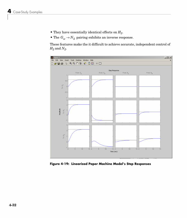
4 Case-Study Examples
4-3
• They have essentially identical effects on H2.
• The pairing exhibits an inverse response.
These features make the it difficult to achieve accurate, independent control of H2 and N2.
Figure 4-19: Linearized Paper Machine Model’s Step Responses
Gw N2→
2

Paper Machine Process Control
MPC DesignType
mpctool
to open the mpc design tool. Import your LTI PaperMach model as described in “Opening MPCTOOL and Importing a Model” on page 4-6.
Next, define signal properties, being sure to designate Np and Nw as measured and unmeasured disturbances, respectively. Your specifications should resemble Figure 4-20.
Figure 4-20: Signal Properties for the Paper Machine Application
Initial Controller DesignIf necessary, review “Specifying Controller Properties” on page 4-10. Then click the MPC1 node and specify the following controller parameters (leaving others at their default values):
• Models and Horizons. Control interval = 2 minutes
• Constraints. For both Gp and Gw, Minimum = -10, Maximum = 10, Max down rate = -2, Max up rate = 2.
4-33
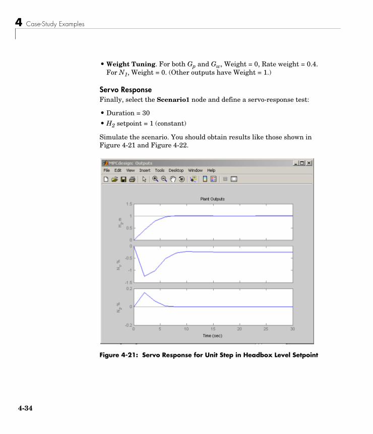
4 Case-Study Examples
4-3
• Weight Tuning. For both Gp and Gw, Weight = 0, Rate weight = 0.4. For N1, Weight = 0. (Other outputs have Weight = 1.)
Servo ResponseFinally, select the Scenario1 node and define a servo-response test:
• Duration = 30
• H2 setpoint = 1 (constant)
Simulate the scenario. You should obtain results like those shown in Figure 4-21 and Figure 4-22.
Figure 4-21: Servo Response for Unit Step in Headbox Level Setpoint
4

Paper Machine Process Control
Figure 4-22: Manipulated Variable Moves Corresponding to Figure 4-21
Weight Tuning The response time is about 8 minutes. We could reduce this by decreasing the control interval, reducing the rate weight on the manipulated variables, and/or eliminating the up/down rate constraints. The present design uses a conservative control effort, which would usually improve robustness, so we will continue with the current settings.
Note the steady-state error in N1 (it’s about -0.25 units in Figure 4-21). There are only two manipulated variables, so it’s impossible to hold three outputs at setpoints. We don’t need to hold N1 so we have set its weight to zero (see controller settings in “Initial Controller Design” on page 4-33). Otherwise, all three outputs would have exhibited steady-state error (try it).
4-35

4 Case-Study Examples
4-3
Consistency control is more important than level control. Try decreasing the H2 weight from 1 to 0.2. You should find that the peak error in N2 decreases by almost an order of magnitude, but the H2 response time increases from 8 to about 18 minutes (not shown). Use these modified output weights in subsequent tests.
Feedforward ControlTo configure a test of the controller’s feedforward response, define a new scenario by clicking on the Scenarios node, clicking the New button, and renaming the new scenario Feedforward (by editing its name in the tree or the summary list).
In the Feedforward scenario, define a step change in the measured disturbance, Np, with Initial value = 0, Size = 1, Time = 10. All output setpoints should be zero. Set the Duration to 30 time units.
If response plots from the above servo response tests are still open, close them. Simulate the Feedforward scenario. You should find that the H2 and N2 outputs deviate very little from their setpoints (not shown).
Experiment with the “look ahead” feature. First, observe that in the simulation just completed the manipulated variables didn’t begin to move until the disturbance occurred at t = 10 minutes. Return to the Feedforward scenario, select the Look ahead option for the measured disturbance, and repeat the simulation.
Notice that the manipulated variables begin changing in advance of the disturbance. This happens because the look ahead option uses known future values of the disturbance when computing its control action. For example, at time t = 0 the controller is using a prediction horizon of 10 control intervals (20 time units), so it “sees” the impending disturbance at t = 10 and begins to prepare for it. The output setpoint tracking improves slightly, but it was already so good that the improvement is insignificant. Also, it’s unlikely that there would be advanced knowledge of a consistency disturbance, so clear the Look ahead check box for subsequent simulations.
Unmeasured Input DisturbanceTo test the response to unmeasured disturbances, define another new scenario called Feedback. Configure it as for Feedforward, but set the measured disturbance, Np, to zero (constant), and the unmeasured disturbance, Nw, to
6

Paper Machine Process Control
1.0 (constant). This simulates a sudden, sustained, unmeasured disturbance occurring at time zero.
Running the simulation should yield results like those in Figure 4-23. The two controlled outputs (H2 and N2) exhibit relatively small deviations from their setpoints (which are zero). The settling time is longer than for the servo response (compare to Figure 4-21) which is typical.
Figure 4-23: Feedback Scenario: Unmeasured Disturbance Rejection
One factor limiting performance is the chosen control interval of 2 time units. The controller can’t respond to the disturbance until it first appears in the outputs, i.e., at t = 2. If you wish, experiment with larger and smaller intervals (modify the specification on the controller’s Model and Horizons tab).
4-37

4 Case-Study Examples
4-3
Effect of Estimator AssumptionsAnother factor influencing the response to unmeasured disturbances (and model prediction error) is the estimator configuration. The results shown in Figure 4-23 are for the default configuration.
To view the default assumptions, select the controller node (MPC1), and select its Estimation tab. The resulting view should be as shown in Figure 4-24. The status message (bottom of figure) indicates that the MPC Toolbox default assumptions are being used.
Figure 4-24: Default Estimator Assumptions: Output Disturbances.
Now consider the upper part of the figure. The Output Disturbances tab is active, and its Signal-by-signal option is selected. According to the tabular data, the controller is assuming independent, step-like disturbances (i.e., integrated white noise) in the first two outputs.
Select the Input Disturbances tab. Verify that the controller is also assuming independent step-like disturbances in the unmeasured disturbance input.
8

Paper Machine Process Control
Thus, there are a total of three independent, sustained (step-like) disturbances. This allows the controller to eliminate offset in all three measured outputs.
The disturbance magnitudes are unity by default. Making one larger than the rest would signify a more important disturbance at that location.
Select the Measurement Noise tab. Verify that white noise (unit magnitude) is being added to each output. The noise magnitude governs how much influence each measurement has on the controller’s decisions. For example, if a particular measurement is relatively noisy, the controller will give it less weight, relying instead upon the model predictions of that output. This provides a noise filtering capability.
In the paper machine application, the default disturbance assumptions are reasonable. It is difficult to improve disturbance rejection significantly by modifying them.
Controlling the Nonlinear Plant in SimulinkIt’s good practice to run initial tests using the linear plant model as described in “Servo Response” on page 4-34, and “Unmeasured Input Disturbance” on page 4-36. Such tests don’t introduce prediction error, and are a useful benchmark for more demanding tests with a nonlinear plant model. The controller’s prediction model is linear, so such tests introduce prediction error.
Figure 4-25: Paper Machine Headbox Control Using MPC Tools in Simulink
4-39

4 Case-Study Examples
4-4
Figure 4-25 is a Simulink diagram in which the MPC Toolbox controller is being used to regulate the nonlinear paper machine headbox model. The block labeled S-Function embodies the nonlinear model, which is coded in an M-file called mpc_pmmodel.m.
As shown in the dialog below, the MPC Controller block references a controller design called MPC1, which was exported to the MATLAB workspace from the design tool. Note also that the measured disturbance inport is enabled, allowing the measured disturbance to be connected as shown in Figure 4-25.
Figure 4-26 shows the scope display from the “Outputs” block for the setup of Figure 4-25, i.e., an unmeasured disturbance. The yellow curve is H2, the
0

Paper Machine Process Control
magenta is N1, and the cyan is N2. Comparing to Figure 4-23, the results are almost identical, indicating that the effects of nonlinearity and prediction error were insignificant in this case. Figure 4-27 shows the corresponding manipulated variable moves (from the “MVs” scope in Figure 4-25) which are smooth yet reasonably fast.
As disturbance size increases, nonlinear effects begin to appear. For a disturbance size of 4, the results are still essentially the same as shown in Figure 4-26 and Figure 4-27 (scaled by a factor of 4), but for a disturbance size of 6, the setpoint deviations are relatively larger, and the curve shapes differ (not shown). There are marked qualitative and quantitative differences when the disturbance size is 8. When it is 9, deviations become very large, and the MVs saturate. If such disturbances were likely, the controller would have to be retuned to accommodate them.
Figure 4-26: Simulink Test: Output Variables
4-41

4 Case-Study Examples
4-4
Figure 4-27: Simulink Test: Manipulated Variables
2

Reference
Reference[1] Ying, Y., M. Rao, and Y. Sun “Bilinear control strategy for paper making process,” Chemical Engineering Communications (1992), Vol. 111, pp. 13-28.
4-43

4 Case-Study Examples
4-4
4
5
The Design Tool
This chapter is the reference manual for the MPC Toolbox design tool (graphical user interface). For example design tool applications, see the MPC Toolbox “Getting Started” manual, or Chapter 4, “Case-Study Examples.” in this document.
Opening the MPC Design Tool (p. 5-2) How to start the design tool from MATLAB or Simulink
The Menu Bar (p. 5-3) Describes the main menu options
The Tool Bar (p. 5-6) Describes the tool bar icons and their use
The Tree View (p. 5-7) Explains how to navigate among the various design tool views
Importing a Plant Model (p. 5-9) The plant model import dialog and its options
Importing a Controller (p. 5-15) The controller import dialog and its options
Exporting a Controller (p. 5-19) The controller export dialog and its options
Signal Definition View (p. 5-21) Detailed description of the initial design tool view, which defines the overall controller structure
Plant Models View (p. 5-26) Lists the plant models available to your design, and allows you to import others
Controllers View (p. 5-29) Lists the controllers in your design and allows you to copy, export, rename, or delete a controller
Simulation Scenarios List (p. 5-33) Lists the simulation scenarios in your design
Controller Specifications View (p. 5-36) Shows how to specify a controller
Simulation Scenario View (p. 5-59) Shows how to set up a simulation
Response Plots (p. 5-67) Describes the plots generated in a simulation and their customization

5 The Design Tool
5-2
Opening the MPC Design ToolTo open the Design Tool in MATLAB, type
mpctool
The design tool is part of the Control and Estimation Tools Manager. When invoked as shown above, the design tool opens as a new project named MPCdesign.
If you started the tool previously, the above command makes the tool visible but doesn’t open a new project.
Alternatively, if your Simulink model contains an MPC Controller block, you can double-click on the block to obtain its mask (see example below) and click the Design button. If the MPC controller field is empty, the design tool will initialize a default controller. Otherwise, it will load the specified existing controller object so you can edit its properties.

The Menu Bar
The Menu BarThe design tool’s menu bar appears whenever you’ve selected an MPC Toolbox project or task in the tree (see “The Tree View” on page 5-7). The menu bar’s MPC option distinguishes it from other control and estimation tools. See the example below. The following sections describe each menu option.
File Menu
New DesignCreates a new (empty) MPC Toolbox design project within the Control and Estimation Tools Manager and assigns it a default name. You can also create a new design using the tool bar (see “The Tool Bar” on page 5-6).
LoadLoads a saved design. A dialog asks you to specify the MAT-file containing the saved design. If the MAT-file contains multiple projects, you must select the one(s) to be loaded (see example below).
You can also load a design using the tool bar (see “The Tool Bar” on page 5-6).
5-3

5 The Design Tool
5-4
SaveSaves a design so you can use it later. The data are saved in a MAT-file. A dialog allows you to specify the file name (see below). If you are working on multiple projects, you can select those to be saved.
You can also select the Save option using the tool bar (see “The Tool Bar” on page 5-6)
CloseCloses the design tool. If you’ve modified the design, you’ll be asked whether or not you want to save it before closing.
MPC Menu
ImportYou have the following options:
• Plant model – Import a plant model using the model import dialog (see “Importing a Plant Model” on page 5-9)
• Controller – Import a controller using the controller import dialog (see “Importing a Controller” on page 5-15)

The Menu Bar
ExportExport a controller using the export dialog (see “Exporting a Controller” on page 5-19). This option won’t be enabled until your design includes at least one fully specified controller.
SimulateSimulate the current scenario, i.e., the one most recently simulated or selected in the tree (see “The Tree View” on page 5-7). You can select this option from the keyboard by typing Ctrl-R, or using the tool bar icon (see “The Tool Bar” on page 5-6).
The Simulate option won’t be unabled until your design includes at least one fully specified simulation scenario.
5-5

5 The Design Tool
5-6
The Tool BarThe tool bar provides quick access to the menu options you’ll use most often.
For more information on each option, see the following:
• “New Design” on page 5-3
• “Load” on page 5-3
• “Save” on page 5-4
• “Simulate” on page 5-5
New Design
Load Saved Design Save Current Design
Simulate CurrentScenario

The Tree View
The Tree ViewThe tree view appears in a frame on the design tool’s left-hand side (see example below). When you select one of the tree’s nodes (by clicking its name or icon) the larger frame to its right shows a dialog panel that allows you to view and edit the specifications associated with that item.
Node Types
The above example shows two MPC Toolbox design project nodes, DistillationControl and CSTRcontrol, and their sub-nodes. For more details on each node type, see the following:
• MPC design project/task – see “Signal Definition View” on page 5-21
• Plant models list – see “Plant Models View” on page 5-26
• Controllers list – see “Controllers View” on page 5-29
• Controller specifications – see “Simulation Scenarios List” on page 5-33
• Scenarios list – see “Simulation Scenario View” on page 5-59
• Scenario specifications – see “Controller Specifications View” on page 5-36
MPC project nodes
Plant models list
Controllers list
Controller specifications
Simulation scenarios list
Scenario specifications
5-7

5 The Design Tool
5-8
Renaming a NodeYou can rename following node types:
• MPC design project/task
• Controller specifications
• Scenario specifications
To rename a node, do one of the following:
• Click on the name, wait for an edit box to appear, type the desired name, and push the Enter key to finalize your choice, OR
• Right-click on the name, select the Rename menu option, and enter the desired name in the dialog box, OR
• To rename a controller specification node, select Controllers and edit the controller name in the table, OR
• To rename a scenario specification node, select Scenarios and edit the scenario name in the table

Importing a Plant Model
Importing a Plant ModelTo import a plant model, do one of the following:
• Select the MPC/Import/Plant Model menu option, OR
• Select the MPC project/task node in the tree (see “The Tree View” on page 5-7), and then click the Import Plant button, OR
• Right-click the MPC project/task node and select the Import Plant Model menu option, OR
• If you’ve already imported a model, select the Plant models node, and then click the Import button, OR
• If you’ve already imported a model, right-click the Plant models node and select the Import Model menu option
All of the above open the Plant Model Importer dialog, shown below. Within the dialog you can import an LTI model from the workspace or, when you have Simulink Control Design, you can import a linearized plant model from the Simulink model. The following sections describe the dialog options for importing an LTI model from the workspace. For information on importing a linearized plant model, see “Importing a Linearized Plant Model” on page 5-12.
5-9

5 The Design Tool
5-1
Import fromUse the radio buttons to set the location from which the model will be imported.
MATLAB Workspace
This is the default option and is the case shown in the above example. The Items in your Workspace area in dialog’s upper-right lists all candidate models in your MATLAB workspace. Select one by clicking on it. The dialog’s Properties area lists the selected model’s properties (the DC model in the above example).
0

Importing a Plant Model
MAT-FileThe upper part of the dialog changes as shown below
The MAT file name edit box becomes active. Type the desired MAT-file name here (if it’s not on the MATLAB path, enter the complete path to the file). You can also use the Browse button which activates a standard file chooser dialog.
In the above example, file DCmodels.mat contains two models. Their names appear in the Items in your MAT file area on the dialog’s upper right. As with the workspace option, the selected model’s properties appear in the Properties area.
Import toThe combo box at the dialog’s bottom allows you to specify the MPC project/task into which the plant model will be imported (see example below). It defaults to the project/task most recently active.
Buttons
ImportSelect the model you want to import from the Items list in the dialog’s upper right. Verify that the Import To option designates the correct project/task. Click the Import button to import the model.
5-11

5 The Design Tool
5-1
You can select Plant models in the tree to verify that the model has been loaded. (see “The Tree View” on page 5-7, and “Plant Models View” on page 5-26).
The import dialog remains visible until you close it, allowing you to import additional models.
CloseClick Close to close the dialog window. You can also click the close icon on the window’s title bar.
Importing a Linearized Plant ModelTo import a linearized plant model from the Simulink model, select the Linearized Plant from Simulink panel within the Plant Model Importer, as shown in the following figure.
2

Importing a Plant Model
Linearization ProcessWhen you click OK, the MPC Toolbox works with Simulink Control Design to create a linearized plant model by automatically performing the following tasks:
1 Configures the Control and Estimation Tools Manager.
2 Temporarily inserts linearization input and output points in the model at the inputs and outputs of the MPC Controller block.
3 When the Create a new operating condition from MPC I/O values is selected, the MPC Toolbox temporarily inserts output constraints at the inputs/outputs of the MPC Controller block..
4 Finds an equilibrium operating condition based on the constraints or uses the specified operating condition.
5 Linearizes the plant model about the operating point.
The linearized plant model is added as a new node under the Plant Models node within the Control and Estimation Tools Manager. For more information on the linearization process, refer to the Simulink Control Design documentation.
Linearization OptionsYou can also customize the linearization process in several ways before clicking OK:
• To specify an alternative name for the linearized plant model, enter the name in the Linearization model name edit field.
• To use an alternative operating condition, you can
- select one from the menu next to Use the previously computed operating condition. This list contains all operating conditions that exist within the current project.
- select Create a new operating condition from MPC I/O values to compute an operating condition by optimization, using the nominal plant values as constraints.
5-13

5 The Design Tool
5-1
• To replace the nominal plant values with the operating point used in the linearization, select the check box next to Replace the MPC nominal I/O values with those derived from the operating condition.
• When there are multiple MPC Controller blocks, use the Import to menu to select a node within the Control and Estimation Tools Manager to import the plant model to.
In addition, the Linearization I/O panel displays the current linearization input and output points in the model. When creating the linearized model, the MPC Toolbox temporarily modifies these input and output points with input and output points suitable for extracting a linearized plant model.
4

Importing a Controller
Importing a ControllerTo import a controller, do one of the following:
• Select the MPC/Import/Controller menu option, OR
• Select the MPC project/task node in the tree (see “The Tree View” on page 5-7), and then click the Import Controller button, OR
• Right-click the MPC project/task node and select the Import Controller menu option, OR
• If you’ve already designed a controller, select the Controllers node, and then click the Import button, OR
• If you’ve already designed a controller, right-click the Controllers node and select the Import Controller menu option
All of the above open the MPC Controller Importer dialog. The following sections describe the dialog’s options.
5-15

5 The Design Tool
5-1
Import fromUse the radio buttons to set the location from which the controller will be imported.
MATLAB Workspace
This is the default option and is the case shown in the above example. The Items in your Workspace area in dialog’s upper-right lists all mpc objects in your workspace. Select one by clicking on it. The Properties area lists the properties of the selected model (the DC model in the above example).
6

Importing a Controller
MAT-FileThe upper part of the dialog changes as shown below
The MAT file name edit box becomes active. Type the desired MAT-file name here (if it’s not on the MATLAB path, enter the complete path to the file). You can also use the Browse button which activates a standard file chooser dialog.
In the above example, file Controllers.mat contains two mpc objects. Their names appear in the Items in your MAT file area on the dialog’s upper right.
Import toThe combo box at the dialog’s bottom allows you to specify the MPC project/task into which the controller will be imported (see example below). It defaults to the project/task most recently active.
Buttons
ImportSelect the controller you want to import from the Items list in the dialog’s upper right. Verify that the Import To option designates the correct project/task. Click the Import button to import the controller.
The new controller should appear in the tree as a sub-node of Controllers. (see “The Tree View” on page 5-7).
The imported controller contains a plant model, which appears in the Plant models list. (see “Plant Models View” on page 5-26).
5-17

5 The Design Tool
5-1
Note If the selected controller is incompatible with any others in the designated project, the design tool will not import it.
The dialog remains visible until you close it, allowing you to import additional models.
CloseClick Close to close the dialog window. You can also click the close icon on the window’s title bar.
8
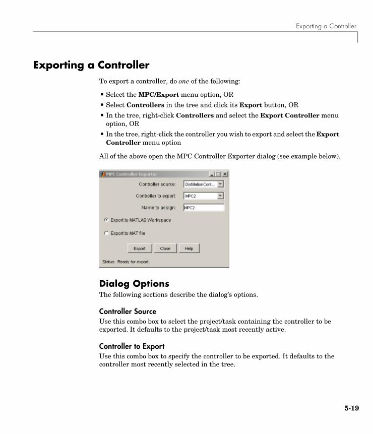
Exporting a Controller
Exporting a ControllerTo export a controller, do one of the following:
• Select the MPC/Export menu option, OR
• Select Controllers in the tree and click its Export button, OR
• In the tree, right-click Controllers and select the Export Controller menu option, OR
• In the tree, right-click the controller you wish to export and select the Export Controller menu option
All of the above open the MPC Controller Exporter dialog (see example below).
Dialog OptionsThe following sections describe the dialog’s options.
Controller SourceUse this combo box to select the project/task containing the controller to be exported. It defaults to the project/task most recently active.
Controller to ExportUse this combo box to specify the controller to be exported. It defaults to the controller most recently selected in the tree.
5-19

5 The Design Tool
5-2
Name to AssignUse this edit box to assign a valid MATLAB variable name (no spaces, etc.). It defaults to a blank-free version of the selected controller’s name.
Export to WorkspaceSelect this radio button if you want the controller to be exported to the MATLAB workspace.
Export to MAT FileSelect this radio button if you want the controller to be exported to a MAT file.
Buttons
ExportIf you’ve selected the to Workspace option, clicking Export causes a new mpc object to be created in your MATLAB workspace. (If one having the assigned name already exists, you’ll be asked if you want to overwrite it.) You can use the MATLAB whos command to verify that the controller has been exported.
If you’ve selected the to MAT File option, clicking Export opens a standard file chooser that allows you to specify the file.
In either case, the dialog window remains visible, allowing you to export additional controllers.
CloseClick Close to close the dialog window. You can also click the close icon on the window’s title bar.
0

Signal Definition View
Signal Definition ViewThe signal definition view appears whenever you select an MPC Toolbox project/task node in the tree (see “The Tree View” on page 5-7). It is also the view you’ll see when you open the design tool for the first time. An example appears below
The following sections describe the view’s main features.
5-21

5 The Design Tool
5-2
MPC Structure OverviewThis upper section is a non-editable display of your application’s structure. Once you’ve imported a plant model (or controller), the graphic shows counts for the five possible signal types, as in the example below
The counts will change if you edit the signal types.
Buttons
Import PlantClicking this opens the Plant Model Importer dialog (see “Importing a Plant Model” on page 5-9).
Import ControllerClicking this opens the MPC Controller Importer dialog (see “Importing a Controller” on page 5-15).
Note You won’t be allowed to proceed with your design until you import a plant model. You can do so indirectly by importing a controller or loading a saved project.
Signal Properties TablesTwo tables display the properties of each signal in your design.
2

Signal Definition View
Input Signal PropertiesThe plant’s input signals appear as table rows (see example below).
The table’s columns are editable and have the following significance:
• Name – The signal name, an alphanumeric string used to label other tables, graphics, etc. Each name must be unique. The design tool assigns a default name if your imported plant model doesn’t specify one.
• Type – One of the three valid MPC Toolbox input signal types. The above example shows one of each. To change a signal’s type, click on the table cell and select the desired type from the resulting menu. The valid signal types are as follows:
Manipulated – A signal that will be manipulated by the controller, i.e., an actuator (valve, motor, etc.)
Measured Disturbance – An independent input whose value is measured and used as a controller input for feedforward compensation
Unmeasured Disturbance – An independent input representing an unknown, unexpected disturbance.
• Description – An optional descriptive string.
• Units – Optional units (dimensions), a string. Used to label other dialogs, simulation plots, etc.
• Nominal – The signal’s nominal value. The design tool defaults this to zero. Any value you assign here will be the default initial condition in simulations.
Note Your design must include at least one manipulated variable. The other input signal types need not be included.
5-23

5 The Design Tool
5-2
Output Signal PropertiesThe plant’s output signals appear as table rows (see example below).
The table’s columns are editable and have the following significance:
• Name – The signal name, an alphanumeric string used to label other tables, graphics, etc. Each name must be unique. The design tool assigns a default name if your imported plant model doesn’t specify one.
• Type – One of the two valid MPC Toolbox output signal types. The above example shows one of each. To change a signal’s type, click on the table cell and select the desired type from the resulting menu. The valid signal types are as follows:
Measured – A signal the controller can use for feedback
Unmeasured – Predicted by the plant model but unmeasured. Can be used as an indicator. Can also be assigned a setpoint or constrained.
• Description – An optional descriptive string.
• Units – Optional units (dimensions), a string. Used to label other dialogs, simulation plots, etc.
• Nominal – The signal’s nominal value. The design tool defaults this to zero. Any value you assign here will be the default initial condition in simulations.
Note Your design must include at least one measured output. Inclusion of unmeasured outputs is optional.
4

Signal Definition View
Right-Click Menu OptionsRight-clicking on an MPC project/task node allows you to choose one of the following menu items:
• Import Plant Model – Opens the Plant Model Importer dialog (see “Importing a Plant Model” on page 5-9)
• Import Controller – Opens the MPC Controller Importer dialog (see “Importing a Controller” on page 5-15)
• Clear Project – Erases all plant models, controllers, and scenarios in your design, returning the project to its initial empty state.
• Delete Project – Deletes the selected project node.
5-25

5 The Design Tool
5-2
Plant Models ViewSelecting Plant models in the tree causes this view to appear (see example below)
The following sections describe the view’s main features.
6

Plant Models View
Plant Models ListThis table lists all the plant models you’ve imported and/or plant models contained in controllers that you’ve imported. The example below lists two imported models, DC and DCp.
The Name field is editable. Each model must have a unique name. The name you assign here will be used within the design tool, but will not alter the original model’s name.
The Type field is noneditable and indicates the model’s LTI object type (see the Control System Toolbox documentation for a detailed discussion of LTI models).
The Sampling Period field is zero for continuous-time models, and a positive real value for discrete-time models.
The Imported on field gives the date and time the model was imported into the design tool.
Model DetailsThis scrollable viewport shows details of the model currently selected in the plant models list (see “Plant Models List” on page 5-27). An example appears below
5-27

5 The Design Tool
5-2
Additional NotesYou can use this editable text area to enter comments, distinguishing model features, etc.
Buttons
ImportOpens the Plant Model Importer dialog (see “Importing a Plant Model” on page 5-9).
DeleteDeletes the selected model. If the model is being used elsewhere (i.e., in a controller or scenario), the first model in the list replaces it (and a warning message appears).
Right-Click OptionsRight-clicking on the Plant models node causes the following menu option to appear
Import ModelOpens the Plant Model Importer dialog (see “Importing a Plant Model” on page 5-9).
8

Controllers View
Controllers ViewSelecting Controllers in the tree causes this view to appear (see example below)
The following sections describe the view’s main features.
5-29
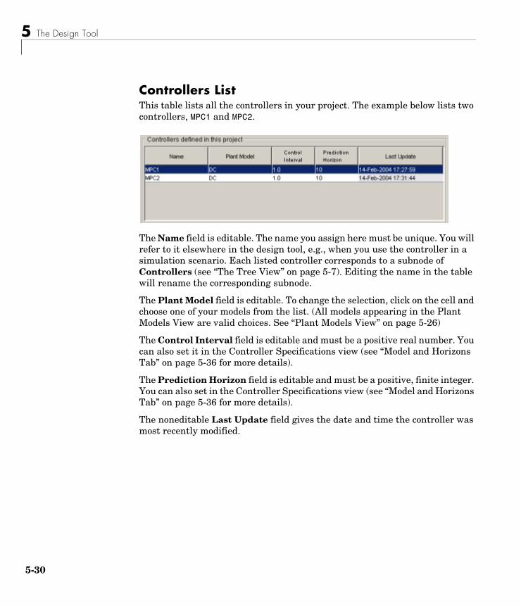
5 The Design Tool
5-3
Controllers ListThis table lists all the controllers in your project. The example below lists two controllers, MPC1 and MPC2.
The Name field is editable. The name you assign here must be unique. You will refer to it elsewhere in the design tool, e.g., when you use the controller in a simulation scenario. Each listed controller corresponds to a subnode of Controllers (see “The Tree View” on page 5-7). Editing the name in the table will rename the corresponding subnode.
The Plant Model field is editable. To change the selection, click on the cell and choose one of your models from the list. (All models appearing in the Plant Models View are valid choices. See “Plant Models View” on page 5-26)
The Control Interval field is editable and must be a positive real number. You can also set it in the Controller Specifications view (see “Model and Horizons Tab” on page 5-36 for more details).
The Prediction Horizon field is editable and must be a positive, finite integer. You can also set in the Controller Specifications view (see “Model and Horizons Tab” on page 5-36 for more details).
The noneditable Last Update field gives the date and time the controller was most recently modified.
0
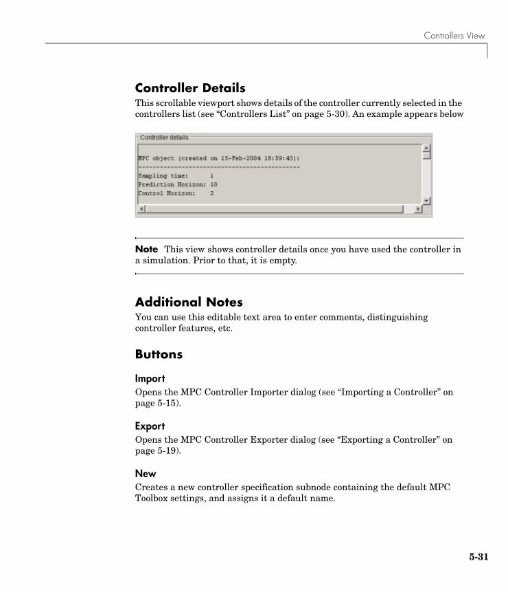
Controllers View
Controller DetailsThis scrollable viewport shows details of the controller currently selected in the controllers list (see “Controllers List” on page 5-30). An example appears below
Note This view shows controller details once you have used the controller in a simulation. Prior to that, it is empty.
Additional NotesYou can use this editable text area to enter comments, distinguishing controller features, etc.
Buttons
ImportOpens the MPC Controller Importer dialog (see “Importing a Controller” on page 5-15).
ExportOpens the MPC Controller Exporter dialog (see “Exporting a Controller” on page 5-19).
NewCreates a new controller specification subnode containing the default MPC Toolbox settings, and assigns it a default name.
5-31

5 The Design Tool
5-3
CopyCopies the selected controller, creating a controller specification subnode containing the same controller settings, and assigning it a default name.
DeleteDeletes the selected controller. If the controller is being used elsewhere (i.e., in a simulation scenario), the first controller in the list replaces it (and a warning message appears).
Right-Click OptionsRight-clicking on the Controllers node causes the following menu options to appear
New ControllerCreates a new controller specification subnode containing the default MPC Toolbox settings, and assigns it a default name.
Import ControllerOpens the MPC Controller Importer dialog (see “Importing a Controller” on page 5-15).
Export ControllerOpens the MPC Controller Exporter dialog (see “Exporting a Controller” on page 5-19).
2

Simulation Scenarios List
Simulation Scenarios ListSelecting Scenarios in the tree causes this view to appear (see example below)
The following sections describe the view’s main features.
5-33

5 The Design Tool
5-3
Scenarios ListThis table lists all the scenarios in your project. The example below lists two, Scenario1 and Scenario2.
The Name field is editable. The assigned name must be unique. Each listed scenario corresponds to a subnode of Scenarios (see “The Tree View” on page 5-7). Editing the name in the table will rename the corresponding subnode.
The Controller field is editable. To change the selection, click on the cell and choose one of your controllers from the list. (All controllers appearing in the Controllers View are valid choices. See “Controllers View” on page 5-29). You can also set this using the Scenario Specifications view (for more discussion, see “Simulation Scenario View” on page 5-59).
The Plant field is editable. To change the selection, click on the cell and choose one of your plant models from the list. (All models appearing in the Plant Models View are valid choices. See “Plant Models View” on page 5-26). You can also set this in the scenario specifications (for more discussion, see “Simulation Scenario View” on page 5-59).
The Closed Loop field is an editable checkbox. If unchecked, the simulation will be open loop. You can also set it in the scenario specifications (for more discussion see “Simulation Scenario View” on page 5-59).
The Constrained field is an editable checkbox. If unchecked, the simulation will ignore all constraints specified in the controller design. You can also set it in the scenario specifications (for more discussion see “Simulation Scenario View” on page 5-59).
The Duration field is editable and must be a positive, finite real number. It sets the simulation duration. You can also set it in the scenario specifications (for more discussion see “Simulation Scenario View” on page 5-59).
4

Simulation Scenarios List
Scenario DetailsThis area is blank at all times.
Additional NotesYou can use this editable text area to enter comments, distinguishing scenario features, etc.
Buttons
NewCreates a new scenario specification subnode containing the default MPC Toolbox settings, and assigns it a default name.
CopyCopies the selected scenario, creating a scenario specification subnode containing the same settings, and assigning it a default name.
DeleteDeletes the selected scenario.
Right-Click OptionsRight-clicking on the Scenarios node causes the following menu option to appear
New ScenarioCreates a new scenario specification subnode containing the default MPC Toolbox settings, and assigns it a default name.
5-35

5 The Design Tool
5-3
Controller Specifications ViewThis view appears whenever you select one of your controller specification nodes (see “The Tree View” on page 5-7). It allows you to specify or review controller settings. It consists of four tabs, each devoted to a particular design aspect. All settings have default values, but these might not be best for your application.
Model and Horizons Tab
6

Controller Specifications View
Plant Model
This combo box allows you to specify the plant model the controller uses for its predictions. You can choose any of the plant models you’ve imported. (See “Importing a Plant Model” on page 5-9.)
Horizons
The Control interval sets the elapsed time between successive controller moves. It must be a positive, finite real number. The calculations assume a zero-order hold on the manipulated variables (the signals adjusted by the controller). Thus, these signals are constant between moves.
The Prediction horizon sets the number of control intervals over which the controller predicts its outputs when computing controller moves. It must be a positive, finite integer.
The Control horizon sets the number of moves computed. It must be a positive, finite integer, and must not exceed the prediction horizon. If less than the prediction horizon, the final computed move fills the remainder of the prediction horizon.
For more discussion, see “A Typical Sampling Instant” on page 1-5, and “Prediction and Control Horizons” on page 1-8.
5-37

5 The Design Tool
5-3
Blocking
By default, the Blocking option is unchecked (off). When on as shown above, the design tool replaces the Control horizon specification (see “Horizons” on page 5-37) with a move pattern determined by the following settings:
• Blocking allocation within prediction horizon – choices are
Beginning – successive moves at the beginning of the prediction horizon, each with a duration of one control interval
Uniform – the prediction horizon is divided by the number of moves and rounded to obtain an integer duration, and each computed move has this duration (the last move extends to fill the prediction horizon)
End – successive moves at the end of the prediction horizon, each with a duration of one control interval
Custom – you specify the duration of each computed move
• Number of moves computed per step – the number of moves computed when the allocation setting is Beginning, Uniform, or End. Must be a positive integer not exceeding the prediction horizon.
• Custom move allocation vector – the duration of each computed move, specified as a row vector. In the example below, there are 4 moves, the first lasting 1 control interval, and the rest lasting 3. The Number of moves computed per step setting is disabled (ignored).
8

Controller Specifications View
The sum of the vector elements should equal the prediction horizon. If not, the last move is extended or truncated automatically.
Note When Blocking is off, the controller uses the Beginning allocation with Number of moves computed per step equal to the Control horizon.
For more discussion, see “Blocking” on page 1-14.
5-39

5 The Design Tool
5-4
Constraints TabThis panel allows you to specify constraints (bounds) on manipulated variables and outputs. Constraints can be hard or soft. By default, all variables are unconstrained, as shown in the view below.
Note If you specify constraints, manipulated variable constraints are hard by default, whereas output variable constraints are soft by default. You can customize this behavior, as discussed in the following sections. For additional information on constraints, see “Optimization and Constraints” on page 1-10, and “Optimization Problem” on page 2-5.
0

Controller Specifications View
Constraints on Manipulated VariablesThe example below is for an application with two manipulated variables (MVs), each represented by a table row.
The Name and Units columns are noneditable. To change them, use the signal definition view. (See “Signal Definition View” on page 5-21. Any changes there apply to the entire design.)
The remaining table columns are editable. If you leave a cell blank, the controller ignores that constraint. You can achieve the same effect by entering -Inf (for a Minimum or Max down rate) or Inf (for a Maximum or Max up rate).
The Minimum and Maximum values set each MV’s range.
The Max down rate and Max up rate values set the amount the MV can change in a single control interval. The Max down rate must be negative or zero. The Max up rate must be positive or zero.
Constraint values must be consistent with your nominal values (see “Input Signal Properties” on page 5-23). In other words, each MV’s nominal value must satisfy the constraints.
Constraint values must also be self-consistent. For example, an MV’s lower bound must not exceed its upper bound.
5-41

5 The Design Tool
5-4
Constraints on Output VariablesThe example below is for an application with two output variables, each represented by a table row.
The Name and Units columns are noneditable. To change them, use the signal definition view. (See “Signal Definition View” on page 5-21. Any changes there apply to the entire design.)
The remaining table columns are editable. If you leave a cell blank (as for the Maximum column above), the controller ignores that constraint. You can achieve the same effect by entering -Inf (for a Minimum) or Inf (for a Maximum).
The Minimum and Maximum values set each output’s range. The controller will attempt to satisfy these constraints at all times.
Constraint values must be consistent with your nominal values (see “Output Signal Properties” on page 5-24). In other words, each output’s nominal value must satisfy the constraints.
Constraint values must also be self-consistent. For example, an output’s lower bound must not exceed its upper bound.
Note Don’t constrain outputs unless a particular constraint is an essential aspect of your application. It is usually better to define output setpoints (reference values) rather than constraints.
2

Controller Specifications View
Constraint SofteningA hard constraint cannot be violated. Hard constraints are risky, especially for outputs, because the controller will ignore its other objectives in order to satisfy them. The constraints might be impossible to satisfy in certain situations, in which case the controllers calculations are mathematically infeasible.
The MPC Toolbox allows you to specify soft constraints. These can be violated, but you specify a violation tolerance for each constraint (the relaxation band). See the example specifications below.
To open this dialog, click the Constraint softening button at the bottom of the Contraints tab in the controller specification view (see “Constraints Tab” on page 5-40).
5-43

5 The Design Tool
5-4
Input ConstraintsAn example input constraint specification appears below.
The Name and Units columns are noneditable. To change them, use the signal definition view. (See “Signal Definition View” on page 5-21. Any changes there apply to the entire design.)
The Minimum, Maximum, Max down rate, and Max up rate columns are editable. Their values are the same as on the main Constraints tab (see “Constraints on Manipulated Variables” on page 5-41). You can specify them in either location.
The remaining columns specify the relaxation band for each constraint. An empty cell is equivalent to a zero, i.e., a hard constraint.
Entries must be zero or positive real numbers. To soften a constraint, increase its relaxation band.
The example above shows a relaxation band of 2 moles/min for the steam flow rate’s lower and upper bounds. The lack of a relaxation band setting for the reflux flow rate’s four constraints means that these will be hard.
Note The relaxation band is a relative tolerance, not a strict bound. In other words, the actual constraint violation can exceed the relaxation band.
4

Controller Specifications View
Output ConstraintsAn example output constraint specification appears below.
The Name and Units columns are noneditable. To change them, use the signal definition view. (See “Signal Definition View” on page 5-21. Any changes there apply to the entire design.)
The Minimum and Maximum columns are editable. Their values are the same as on the main Constraints tab (see “Constraints on Output Variables” on page 5-42). You can specify them in either location.
The remaining columns specify the relaxation band for each constraint. An empty cell is equivalent to 1.0, i.e., a soft constraint.
Entries must be zero or positive real numbers. To soften a constraint, increase its relaxation band.
The example above shows a relaxation band of 0.5 Mole % for the distillate purity lower bound, and a relaxation band of 0.2 Mole % for the bottoms purity lower bound (the harder of the two constraints).
Note The relaxation band is a relative tolerance, not a strict bound. In other words, the actual constraint violation can exceed the relaxation band.
5-45

5 The Design Tool
5-4
Overall Constraint SoftnessThe relaxation band settings allow you to adjust the hardness/softness of each constraint. You can also soften/harden all constraints simultaneously using the slider at the bottom of the dialog panel.
You can move the slider or edit the value in the edit box, which must be between 0 and 1.
ButtonsOK – Closes the constraint softening dialog, implementing changes to the tabular entries or the slider setting.
Cancel – Closes the constraint softening dialog without changing anything.
6

Controller Specifications View
Weight Tuning TabThe example below shows the MPC Toolbox default tuning weights for an application with two manipulated variables and two outputs.
The following sections discuss the three panel areas in more detail. For additional information, see “Optimization Problem” on page 2-5.
5-47
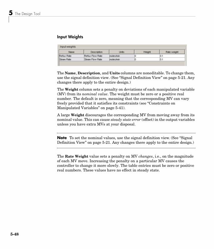
5 The Design Tool
5-4
Input Weights
The Name, Description, and Units columns are noneditable. To change them, use the signal definition view. (See “Signal Definition View” on page 5-21. Any changes there apply to the entire design.)
The Weight column sets a penalty on deviations of each manipulated variable (MV) from its nominal value. The weight must be zero or a positive real number. The default is zero, meaning that the corresponding MV can vary freely provided that it satisfies its constraints (see “Constraints on Manipulated Variables” on page 5-41).
A large Weight discourages the corresponding MV from moving away from its nominal value. This can cause steady state error (offset) in the output variables unless you have extra MVs at your disposal.
Note To set the nominal values, use the signal definition view. (See “Signal Definition View” on page 5-21. Any changes there apply to the entire design.)
The Rate Weight value sets a penalty on MV changes, i.e., on the magnitude of each MV move. Increasing the penalty on a particular MV causes the controller to change it more slowly. The table entries must be zero or positive real numbers. These values have no effect in steady state.
8
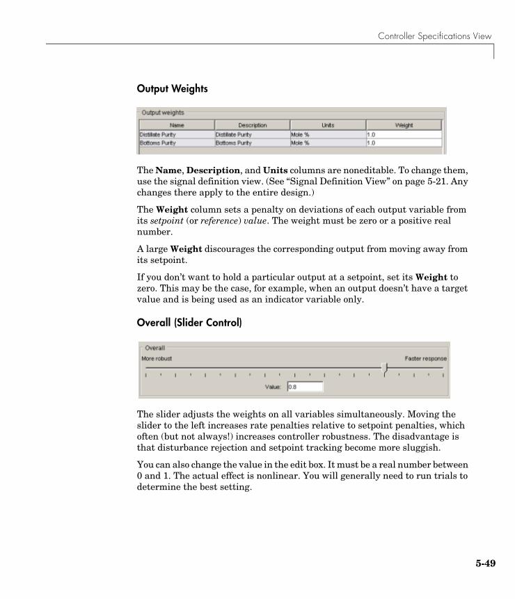
Controller Specifications View
Output Weights
The Name, Description, and Units columns are noneditable. To change them, use the signal definition view. (See “Signal Definition View” on page 5-21. Any changes there apply to the entire design.)
The Weight column sets a penalty on deviations of each output variable from its setpoint (or reference) value. The weight must be zero or a positive real number.
A large Weight discourages the corresponding output from moving away from its setpoint.
If you don’t want to hold a particular output at a setpoint, set its Weight to zero. This may be the case, for example, when an output doesn’t have a target value and is being used as an indicator variable only.
Overall (Slider Control)
The slider adjusts the weights on all variables simultaneously. Moving the slider to the left increases rate penalties relative to setpoint penalties, which often (but not always!) increases controller robustness. The disadvantage is that disturbance rejection and setpoint tracking become more sluggish.
You can also change the value in the edit box. It must be a real number between 0 and 1. The actual effect is nonlinear. You will generally need to run trials to determine the best setting.
5-49

5 The Design Tool
5-5
Estimation TabUse these specifications to shape the controller’s response to unmeasured disturbances and measurement noise.
The example below shows the MPC Toolbox default settings for an application with two output variables and no unmeasured disturbance inputs.
The following sections cover each estimation feature in detail. For additional information, see “State Estimation” on page 1-13, and “State Estimation” on page 2-8.
0

Controller Specifications View
Button (MPC Default Settings)If you edit any of the Estimation tab settings, the display near the top will appear as follows
To return the settings to the default state, click the Use MPC defaults button, causing the display to revert to the default condition shown below
Overall Estimator Gain
This slider determines the controller’s overall disturbance response. As you move the slider to the left, the controller responds less aggressively to unexpected changes in the outputs, i.e., it assumes that such changes are more likely to be caused by measurement noise rather than a real disturbance.
You can also change the value in the edit box. It must be between zero and 1. The effect is nonlinear, and you might need to run trial simulations to achieve the desired result.
5-51

5 The Design Tool
5-5
Output DisturbancesUse these settings to model unmeasured disturbances adding to the plant outputs.
The example below shows the tab’s appearance with the Signal-by-signal option selected for an application having two plant outputs.
The graphic shows the disturbance location.
Use the table to specify the disturbance character for each output.
The Name and Units columns are noneditable. To change them, use the signal definition view. (See “Signal Definition View” on page 5-21. Any changes there apply to the entire design.)
The Type column sets the disturbance character. To edit this, click the cell and select from the resulting menu. You have the following options:
• Steps – simulates random step-like disturbances (integrated white noise)
• Ramps – simulates a random drifting disturbance (doubly-integrated white noise)
2
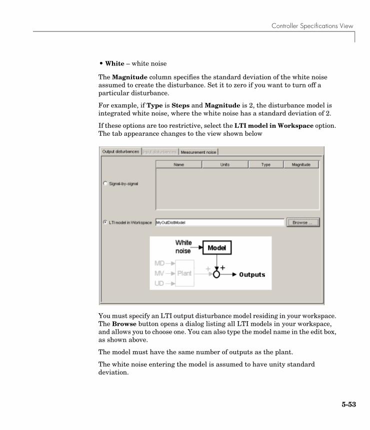
Controller Specifications View
• White – white noise
The Magnitude column specifies the standard deviation of the white noise assumed to create the disturbance. Set it to zero if you want to turn off a particular disturbance.
For example, if Type is Steps and Magnitude is 2, the disturbance model is integrated white noise, where the white noise has a standard deviation of 2.
If these options are too restrictive, select the LTI model in Workspace option. The tab appearance changes to the view shown below
You must specify an LTI output disturbance model residing in your workspace. The Browse button opens a dialog listing all LTI models in your workspace, and allows you to choose one. You can also type the model name in the edit box, as shown above.
The model must have the same number of outputs as the plant.
The white noise entering the model is assumed to have unity standard deviation.
5-53

5 The Design Tool
5-5
Input DisturbancesUse these settings to model disturbances affecting the plant’s unmeasured disturbance inputs.
The example below shows the tab’s appearance with the Signal-by-signal option selected for a plant having one unmeasured disturbance input. The graphic shows the disturbance location.
Use the table to specify the character of each unmeasured disturbance input.
The Name and Units columns are noneditable. To change them, use the signal definition view. (See “Signal Definition View” on page 5-21. Any changes there apply to the entire design.)
The Type column sets the disturbance character. To edit this, click the cell and select from the resulting menu. You have the following options:
• Steps – simulates random step-like disturbances (integrated white noise)
• Ramps – simulates a random drifting disturbance (doubly-integrated white noise)
4
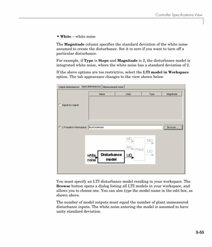
Controller Specifications View
• White – white noise
The Magnitude column specifies the standard deviation of the white noise assumed to create the disturbance. Set it to zero if you want to turn off a particular disturbance.
For example, if Type is Steps and Magnitude is 2, the disturbance model is integrated white noise, where the white noise has a standard deviation of 2.
If the above options are too restrictive, select the LTI model in Workspace option. The tab appearance changes to the view shown below
You must specify an LTI disturbance model residing in your workspace. The Browse button opens a dialog listing all LTI models in your workspace, and allows you to choose one. You can also type the model name in the edit box, as shown above.
The number of model outputs must equal the number of plant unmeasured disturbance inputs. The white noise entering the model is assumed to have unity standard deviation.
5-55
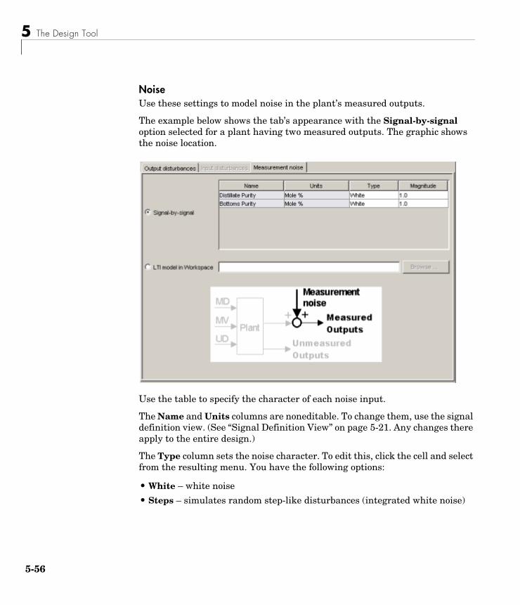
5 The Design Tool
5-5
NoiseUse these settings to model noise in the plant’s measured outputs.
The example below shows the tab’s appearance with the Signal-by-signal option selected for a plant having two measured outputs. The graphic shows the noise location.
Use the table to specify the character of each noise input.
The Name and Units columns are noneditable. To change them, use the signal definition view. (See “Signal Definition View” on page 5-21. Any changes there apply to the entire design.)
The Type column sets the noise character. To edit this, click the cell and select from the resulting menu. You have the following options:
• White – white noise
• Steps – simulates random step-like disturbances (integrated white noise)
6

Controller Specifications View
The Magnitude column specifies the standard deviation of the white noise assumed to create the noise. Set it to zero if you want to specify that an output is noise-free.
For example, if Type is Steps and Magnitude is 2, the noise model is integrated white noise, where the white noise has a standard deviation of 2.
If the above options are too restrictive, select the LTI model in Workspace option. The tab appearance changes as follows
You must specify an LTI model residing in your workspace. The Browse button opens a dialog listing all LTI models in your workspace, and allows you to choose one. You can also type the model name in the edit box, as shown above.
The number of noise model outputs must equal the number of plant measured outputs.
The white noise entering the model is assumed to have unity standard deviation.
5-57

5 The Design Tool
5-5
Right-Click Menus
Copy ControllerCreates a new controller having the same settings and a default name.
Delete ControllerDeletes the controller. If the controller is being used in a simulation scenario, the design tool replaces it with the first controller in your list, and displays a warning message.
Rename ControllerOpens a dialog allowing you to rename the controller.
Note Each controller in a design project/task must have a unique name.
Export ControllerOpens the MPC Controller Exporter dialog (see “Exporting a Controller” on page 5-19).
8
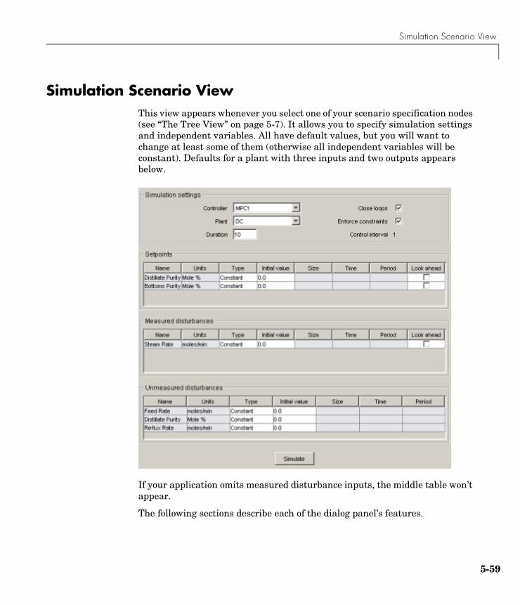
Simulation Scenario View
Simulation Scenario ViewThis view appears whenever you select one of your scenario specification nodes (see “The Tree View” on page 5-7). It allows you to specify simulation settings and independent variables. All have default values, but you will want to change at least some of them (otherwise all independent variables will be constant). Defaults for a plant with three inputs and two outputs appears below.
If your application omits measured disturbance inputs, the middle table won’t appear.
The following sections describe each of the dialog panel’s features.
5-59

5 The Design Tool
5-6
Simulation Settings
Use this section to set the following:
• Controller – select one of your controllers
• Plant – select the plant model that will act as the “real” plant in the simulation, i.e., it need not be the same as that used for controller predictions.
• Duration – the simulation duration in time units
• Close loops – if unchecked, the simulation will be open-loop
• Enforce Constraints – if unchecked, all controller constraints will be ignored
The Control interval field is display-only, and reflects the setting in your Controller selection. You can change it there if necessary (see “Model and Horizons Tab” on page 5-36).
Setpoints
Note Setpoint specifications affect closed-loop simulations only.
Use this table to specify the setpoint for each output. In the example below, which is for an application having two plant outputs, both setpoints would be constant at 0.0.
0

Simulation Scenario View
The Name and Units columns are display-only. To change them, use the signal definition view. (See “Signal Definition View” on page 5-21. Any changes apply to the entire design.)
The Type column specifies the setpoint variation. To change this, click on the cell and select a choice from the resulting menu.
The significance of the Initial value, Size, Time, and Period columns depends on the Type. If a cell is gray (noneditable), it doesn’t apply to the Type you’ve chosen.
For details on the signal types, see “Signal Type Settings” on page 5-64.
If the Look ahead option is checked (i.e., on), the controller will use future values of the setpoints in its calculations. This improves setpoint tracking, but knowledge of future setpoint changes is unusual in practice.
Note In the current implementation, checking or unchecking the Look ahead option for one output will set the others to the same state. The MPC Toolbox code does not allow you to Look ahead for some outputs but not for others.
Measured DisturbancesUse this table to specify the variation of each measured disturbance. In the example below, which is for an application having a single measured disturbance, the “Steam Rate” input would be constant at 0.0.
The Name and Units columns are display-only. To change them, use the signal definition view. (See “Signal Definition View” on page 5-21. Any changes apply to the entire design.)
5-61

5 The Design Tool
5-6
The Type column specifies the disturbance variation. To change this, click on the cell and select a choice from the resulting menu.
The significance of the Initial value, Size, Time, and Period columns depends on the Type. If a cell is gray (noneditable), it doesn’t apply to the Type you’ve chosen.
For details on the signal types, see “Signal Type Settings” on page 5-64.
If the Look ahead option is checked (i.e., on), the controller will use future values of the measured disturbance(s) in its calculations. This improves disturbance rejection, but knowledge of future disturbances is unusual in practice. It has no effect in an open-loop simulation.
Note In the current implementation, checking or unchecking the Look ahead option for one input will set the others to the same state. The MPC Toolbox code does not allow you to Look ahead for some inputs but not for others.
Unmeasured DisturbancesUse this table to specify the variation of each measured unmeasured disturbance. In the example below, all would be constant at 0.0.
Unmeasured Disturbance LocationsYou can cause unmeasured disturbances to occur in any of the following locations:
• The plant’s unmeasured disturbance (UD) inputs (if any)
• The plant’s measured outputs (MO)
• The plant’s manipulated variable (MV) inputs
2

Simulation Scenario View
All of the above will appear as rows in the table. In the case of a measured output or manipulated variable, the disturbance is an additive bias.
The Name and Units columns are display-only. To change them, use the signal definition view. (See “Signal Definition View” on page 5-21. Any changes apply to the entire design.)
The Type column specifies the disturbance variation. To change this, click on the cell and select a choice from the resulting menu.
The significance of the Initial value, Size, Time, and Period columns depends on the Type. If a cell is gray (noneditable), it doesn’t apply to the Type you’ve chosen.
For details on the signal types, see “Signal Type Settings” on page 5-64.
Open-Loop SimulationsFor open-loop simulations, you can vary the MV unmeasured disturbance to simulate the plant’s response to a particular MV. The MV signal coming from the controller stays at its nominal value, and the MV unmeasured disturbance adds to it.
For example, suppose Reflux Rate is an MV, and the corresponding row in the table below represents an unmeasured disturbance in this MV.
You could set it to a constant value of 1 to simulate the plant’s open-loop unit-step response to the Reflux Rate input. (In a closed-loop simulation, controller adjustments would also contribute, changing the response.)
Similarly, an unmeasured disturbance in an MO adds to the output signal coming from the plant. If there are no changes at the plant input, the plant outputs are constant, and you see only the change due to the disturbance. This allows you to check the disturbance character before running a closed-loop simulation.
5-63

5 The Design Tool
5-6
Signal Type SettingsThe table below is an example that uses each of the six available signal types. The cells with white backgrounds are the entries you must supply. All have defaults.
ConstantThe signal value equals the specified Initial value for the entire simulation.
for
StepPrior to Time, the signal = Initial value. At Time, the signal changes step-wise by Size units. Its value thereafter = Initial value + Size.
for where y0 = Initial value, t0 = Time
for where M = Size
RampPrior to Time, the signal = Initial value. At Time, the signal begins to vary linearly with slope Size.
for where y0 = Initial value, t0 = Time
for where M = Size
SinePrior to Time, the signal = Initial value. At Time, the signal begins to vary sinusoidally with amplitude Size and period Period.
y y0= t 0≥
y y0= 0 t t0<≤
y y0 M+= t t0≥
y y0= 0 t t0<≤
y y0 M t t0–( )+= t t0≥
4

Simulation Scenario View
for where y0 = Initial value, t0 = Time
for where M = Size, /Period
PulsePrior to Time, the signal = Initial value. At Time, a square pulse of duration Period and magnitude Size occurs.
for where y0 = Initial value, t0 = Time
for where M = Size, T = Period
for
GaussianPrior to Time, the signal = Initial value. At Time, the signal begins to vary randomly about Initial value with standard deviation Size.
for where y0 = Initial value, t0 = Time
for where M = Size
randn is MATLAB’s random-normal function, which generates random numbers having zero mean and unit variance.
Simulation ButtonClick the Simulate button to simulate the scenario. You can also type ctrl-R, use the tool bar icon (see “The Tool Bar” on page 5-6), or use the MPC/Simulate menu option (see “The Menu Bar” on page 5-3).
Right-Click Menus
Copy ScenarioCreates a new simulation scenario having the same settings and a default name.
y y0= 0 t t0<≤
y y0 M ω t t0–( )[ ]sin+= t t0≥ ω 2π=
y y0= 0 t t0<≤
y y0 M+= t0 t t0 T+<≤
y y0= t t0 T+≥
y y0= 0 t t0<≤
y y0 Mrandn+= t t0≥
5-65
5 The Design Tool
5-6
Delete ScenarioDeletes the scenario.
Rename ScenarioOpens a dialog allowing you to rename the scenario.
Note Each scenario in a design project/task must have a unique name.
6

Response Plots
Response PlotsEach time you simulate a scenario, the design tool plots the corresponding plant input and output responses. The graphic below shows such a response plot for a plant having two outputs (the corresponding input response plot is not shown).
By default, each plant signal plots in its own graph area (as shown above). If the simulation is closed loop, each output signal plot include the corresponding setpoint.
The following sections describe response plot customization options.
Data MarkersYou can use data markers to label a curve or to display numerical details.
5-67

5 The Design Tool
5-6
Adding a Data MarkerTo add a data marker, click on the desired curve at the location you want to mark. The following graph shows a marker added to each output response and its corresponding setpoint.
Data Marker ContentsEach data marker provides information about the selected point, as follows:
• Response – the scenario that generated the curve
• Time – the time value at the data marker location
• Amplitude – the signal value at the data marker location
• Output – the plant variable name (plant outputs only)
• Input – [*** this needs to be fixed ***]
Changing a Data Marker’s AlignmentTo relocate the data marker’s label (without moving the marker), right-click on the marker, and select one of the four Alignment menu options. The above example shows three of the possible four alignment options.
8

Response Plots
Relocating a Data MarkerTo move a marker, left-click on it (holding down the mouse key) and drag it along its curve to the desired location.
Deleting Data MarkersTo delete all data markers in a plot, click in the plot’s white space.
To delete a single data marker, right-click on it and select the Delete option.
Right-Click OptionsRight-click on a data marker to use one of the following options:
• Alignment – relocate the marker’s label
• Font Size – change the label’s font size
• Movable – on/off option that makes the marker movable or fixed
• Delete – deletes the selected marker
• Interpolation – Interplolate linearly between the curve’s data points, or locate at the nearest data point
• Track Mode – Changes the way the marker responds when you drag it
Displaying Multiple ScenariosBy default the response plots include all the scenarios you’ve simulated. The example below shows a response plot for a plant with two outputs. The data markers indicate the two scenarios being plotted: “Accurate Model” and “Perturbed Model”. Both scenarios use the same setpoints (not marked – the lighter solid lines).
Viewing Selected ScenariosIf your plots are too cluttered, you can hide selected scenarios. To do so, right-click in the plot’s white space, choose Responses from the resulting menu, then toggle responses (i.e., scenarios) on or off using the submenu.
Note This selection affects all variables being plotted.
5-69

5 The Design Tool
5-7
Revising a ScenarioIf you modify and recalculate a scenario, its data are replotted, replacing the original curves.
Viewing Selected VariablesBy default, the design tool plots all plant inputs in a single window, and plots all plant outputs in another. If your application involves many signals, the plots of each may be too small to view comfortably.
Therefore, you can control the variables being plotted. To do so, right-click in a plot’s white space and choose I/O Selector from the resulting menu. A dialog box appears, on which you can opt to show or hide each variable.
Grouping Variables in a Single PlotBy default, each variable appears in its own plot area. You can instead choose to display variables together in a single plot. To do so, right-click in a plot’s white space select I/O Grouping, and then select All.
To return to the default mode, use the I/O Grouping: None option.
0

Response Plots
Normalizing Response AmplitudesWhen you’re using the I/O Grouping: All option, you might find that the variables have very different scales, making it very difficult to view them together. You can choose to normalize the curves, so that each expands or contracts to fill the available plot area.
For example, the plot below shows two plant outputs together (I/O Grouping: All option). The outputs have very different magnitudes, so together they plot as nearly straight lines at the extremes of the y-axis scale.
The plot below shows the normalized version, which displays each curve’s variations clearly.
The y-axis scale is no longer meaningful, however. If you want to know a normalized signal’s amplitude, use a data marker (see “Adding a Data Marker” on page 5-68). Note that the two data markers on the plot below are at the same normalized y-axis location, but correspond to very different amplitudes in the original (unnormalized) coordinates.
5-71

5 The Design Tool
5-7
2
6
Function Reference
Functions — Categorical List (p. 6-2) A list of available functions, sorted by category
Functions — Alphabetical List (p. 6-5) A list of available functions, sorted alphabetically

6 Function Reference
6-2
Functions — Categorical List
MPC Controller
MPC Controller Characteristics
Function Name Description
d2d Change MPC controller’s sampling time
display Display properties of MPC controller
get Access/query property values
mpc Create MPC controller
set Set/modify MPC controller properties
setmpcsignals Set signal types in MPC plant model
getname Get I/O signal names in MPC prediction model
setname Set I/O signal names in MPC prediction model
getmpcdata Get privateMPC data structure
setmpcdata Get privateMPC data structure
Function Name Description
compare Compare two MPC objects
isempty Test true for empty MPC controller
mpcprops Provide help on MPC controller’s properties
mpchelp MPC property and function help
mpcverbosity Change the level of verbosity of the MPC Toolbox
pack Reduce size of MPC object in memory
size Display model output/input/disturbance dimensions

Functions — Categorical List
Linear Behavior of MPC Controller
MPC State
MPC Computation and Simulation
Function Name Description
cloffset Compute MPC closed-loop DC gain from output disturbances to measured outputs assuming constraints are inactive at steady state
ss Convert unconstrained MPC controller to state-space linear form
tf Convert unconstrained MPC controller to linear transfer function
zpk Convert unconstrained MPC controller to zero/pole/gain form
Function Name Description
mpcstate Define state for MPC controller
trim Compute the steady-state value of MPC controller state for given inputs and outputs values.
get Access/query MPC state properties
set Set/modify MPC state properties
Function Name Description
mpcmove Compute the MPC control action
sim Simulate closed-loop/open-loop response to arbitrary reference and disturbance signals
mpcsimopt Specify MPC simulation options
plot Plot responses generated by MPC simulations
6-3

6 Function Reference
6-4
State Estimation
Quadratic Programming
Function Name Description
getestim Extract model and gain used for observer design
setestim Modify an MPC object's linear state estimator
getindist Retrieves the unmeasured input disturbance model
setindist Modify the unmeasured input disturbance model
getoutdist Retrieve unmeasured output disturbance model
setoutdist Modify the unmeasured output disturbance model
Function Name Description
qpdantz Solve a convex quadratic program using Dantzig-Wolfe’s algorithm
qpsolver QP solver

Functions — Alphabetical List
6-5
Functions — Alphabetical List 6
This section contains function reference pages listed alphabetically.

cloffset
6cloffsetPurpose Compute MPC closed-loop DC gain from output disturbances to measured outputs assuming constraints are inactive at steady state
Syntax DCgain=cloffset(MPCobj)
Description The cloff function computes the DC-gain from output disturbances to measured outputs, assuming constraints are not active, based on the feedback connection between Model.Plant and the linearized MPC controller, as depicted below.
Computing the Effect of Output Disturbances
By superposition of effects, the gain is computed by zeroing references, measured disturbances, and unmeasured input disturbances.
DCgain=cloffset(MPCobj) returns an nym-by-nym DC gain matrix DCgain, where nym is the number of measured plant outputs. MPCobj is the MPC object specifying the controller for which the closed-loop gain is calculated. DCgain(i,j) represents the gain from an additive (constant) disturbance on output j to measured output i. If row i contains all zeros, there will be no steady-state offset on output i.
6-6

cloffset
Examples See misocloffset.m in mpcdemos
See Also mpc, ss
6-7

compare
6comparePurpose Compare two MPC objects
Syntax yesno=compare(MPC1,MPC2)
Description The compare function compares the contents of two MPC objects MPC1, MPC2. If the design specifications (models, weights, horizons, etc.) are identical, then yesno is equal to 1.
Note compare may return yesno=1 even if the two objects are not identical. For instance, MPC1 may have been initialized while MPC2 may have not, so that they may have different sizes in memory. In any case, if yesno=1 the behavior of the two controllers will be identical.
See Also mpc, pack
6-8

d2d
6d2dPurpose Change MPC controller’s sampling time
Syntax MPCobj=d2d(MPCobj,ts)
Description The d2d function changes the sampling time of the MPC controller MPCobj to ts. All models are sampled or resampled as soon as the QP matrices must be computed, e.g., when sim or mpcmove are used.
See Also mpc, set
6-9

get
6getPurpose Access/query MPC property values
Syntax Value = get(MPCobj,'PropertyName')get(MPCobj)Struct = get(MPCobj)
Description Value = get(MPCobj,'PropertyName') returns the current value of the property PropertyName of the MPC controller MPCobj. The string 'PropertyName' can be the full property name (for example, 'UserData') or any unambiguous case-insensitive abbreviation (for example, 'user'). You can specify any generic MPC property.
Struct = get(MPCobj) converts the MPC controller MPCobj into a standard MATLAB structure with the property names as field names and the property values as field values.
get(MPCobj) without a left-side argument displays all properties of MPCobj and their values.
Remark An alternative to the syntax
Value = get(MPCobj,'PropertyName')
is the structure-like referencing
Value = MPCobj.PropertyName
For example,
MPCobj.TsMPCobj.p
return the values of the sampling time and prediction horizon of the MPC controller MPCobj.
See Also mpc, set
6-10

getestim
6getestimPurpose Extract model and gain used for observer design
Syntax M=getestim(MPCobj)[M,A,Cm]=getestim(MPCobj)[M,A,Cm,Bu,Bv,Dvm]=getestim(MPCobj)
[M,model,Index]=getestim(MPCobj,'sys')
Description M=getestim(MPCobj) extracts the estimator gain M used by the MPC controller MPCobj for observer design. The observer is based on the models specified in MPCobj.Model.Plant, in MPCobj.Model.Disturbance, by the output disturbance model (default is integrated white noise, see “Output Disturbance Model” on page 2-9), and by MPCobj.Model.Noise.
The state estimator is based on the linear model (cf. “State Estimation” on page 2-8)
where v(k) are the measured disturbances, u(k) are the manipulated plant inputs, ym(k) are the measured plant outputs, and x(k) is the overall state vector collecting states of plant, unmeasured disturbance, and measurement noise models.
The estimator used in the MPC Toolbox is described in “State Estimation” on page 2-8. The estimator’s equations are
Predicted Output Computation:
Measurement Update:
Time Update:
By combining these three equations, the overall state observer is
x k 1+( ) Ax k( ) Buu k( ) Bvv k( )++=
ym k( ) Cmx k( ) Dvmv k( )+=
ym k k 1–( ) Cmx k k 1–( ) Dvmv k( )+=
x k k( ) x k k 1–( ) M ym k( ) ym k k 1–( )–( )+=
x k 1 k+( ) Ax k k )( ) Buu k( ) Bvv k( )++=
6-11

getestim
where L=AM.
[M,A,Cm]=getestim(MPCobj) also returns matrices A,Cm used for observer design. This includes plant model, disturbance model, noise model, offsets. The extended state is
x=plant states; disturbance models states; noise model states]
[M,A,Cm,Bu,Bv,Dvm]=getestim(MPCobj) retrieves the whole linear system used for observer design.
[M,model,Index]=getestim(MPCobj,'sys') retrieves the overall model used for observer design (specified in the Model field of the MPC object) as an LTI state-space object, and optionally a structure Index summarizing I/O signal types.
The extended input vector of model model is
u=[manipulated vars;measured disturbances; 1; noise exciting disturbance model;noise exciting noise model]
Model model has an extra measured disturbance input v=1 used for handling possible nonequilibrium nominal values (see “Offsets” on page 2-4).
Input, output, and state names and input/output groups are defined for model model.
The structure Index has the fields detailed in the following table.
Field Name Description
ManipulatedVariables Indices of manipulated variables within input vector
MeasuredDisturbances Indices of measured disturbances within input vector (not including offset=1)
Offset Index of offset=1
WhiteNoise Indices of white noise signals within input vector
x k 1 k+( ) A LCm–( )x k k( ) Lym k( )Buu k( ) Bv LDvm–( )v k( )++=
6-12

getestim
The model returned by getestim does not include the additional white noise added on manipulated variables and measured disturbances to ease the solvability of the Kalman filter design, as described in Equation 2-6 on page 2-10.
See Also setestim, mpc, mpcstate
MeasuredOutputs Indices of measured outputs within output vector
UnmeasuredOutputs Indices of unmeasured outputs within output vector
Field Name Description
6-13
getindist
6getindistPurpose Retrieves the unmeasured input disturbance model
Syntax model=getindist(MPCobj)
Description model=getindist(MPCobj) retrieves the linear discrete-time transfer function used to model unmeasured input disturbances in the MPC setup described by the MPC object MPCobj. Model model is an LTI object with as many outputs as the number of unmeasured input disturbances, and as many inputs as the number of white noise signals driving the input disturbance model.
See Figure 2-2, Model Used for State Estimation, on page 2-8 for details about the overall model used in the MPC algorithm for state estimation purposes.
See Also mpc, setindist, setestim, getestim, getoutdist
6-14

getmpcdata
6getmpcdataPurpose Get private MPC data structure
Syntax mpcdata=getmpcdata(MPCobj)
Description mpcdata=getmpcdata(MPCobj) returns the private field MPCData of the MPC object MPCobj. Here, all internal QP matrices, models, estimator gains are stored at initalization of the object. You can manually change the private data structure using the setmpcdata command, although you may only need this for very advanced use of the MPC Toolbox.
Note Changes to the data structure may easily lead to unpredictable results.
See Also setmpcdata, set, get
6-15

getname
6getnamePurpose Get I/O signal names in MPC prediction model
Syntax name=getname(MPCobj,'input',I)name=getname(MPCobj,'output',I)
Description name=getname(MPCobj,'input',I) returns the name of the I-th input signal in variable name. This is equivalent to name=MPCobj.Model.Plant. InputName{I}. The name property is equal to the contents of the corresponding Name field of MPCobj.DisturbanceVariables or MPCobj.ManipulatedVariables.
name=getname(MPCobj,'output',I) returns the name of the I-th output signal in variable name. This is equivalent to name=MPCobj.Model.Plant.OutputName{I}. The name property is equal to the contents of the corresponding Name field of MPCobj.OutputVariables.
See Also setname, mpc, set
6-16

getoutdist
6getoutdistPurpose Retrieve unmeasured output disturbance model
Syntax outdist=getoutdist(MPCobj)
[outdist,channels]=getoutdist(MPCobj)
Description outdist=getoutdist(MPCobj) retrieves the linear discrete-time transfer function used to model output disturbances in the MPC setup described by the MPC object MPCobj. Model outdist is an LTI object with as many outputs as the number of measured + unmeasured outputs, and as many inputs as the number of white noise signals driving the output disturbance model.
See Figure 2-2, Model Used for State Estimation, on page 2-8 for details about the overall model used in the MPC algorithm for state estimation purposes.
[outdist,channels]=getoutdist(MPCobj) also returns the output channels where integrated white noise was added as an output disturbance model. This is only meaninful when the default output disturbance model is used, namely when MPCobj.OutputVariables(i).Integrators is empty for all channels i. The array channels is empty for user-provided output disturbance models.
See Also mpc, setoutdist, setestim, getestim, getindist
6-17

mpc
6mpcPurpose Create MPC controller
Syntax MPCobj=mpc(plant)MPCobj=mpc(plant,ts)MPCobj=mpc(plant,ts,p,m)MPCobj=mpc(plant,ts,p,m,weights)MPCobj=mpc(plant,ts,p,m,weights,MV,OV,DV)MPCobj=mpc(models,ts,p,m,weights,MV,OV,DV)MPCobj=mpc
Description MPCobj=mpc(plant) creates a MPC controller based on the discrete-time model model plant. The model can be specified either as an LTI object, or as an object in the System Identification Toolbox’s format (IDMODEL object), see Using Identified Models (p. 2-19).
MPCobj=mpc(plant,ts) also specifies the sampling time ts for the MPC controller. A continuous-time plant is discretized with sampling time ts. A discrete-time plant is resampled if its sampling time is different than the controller’s sampling time ts. If plant is a discrete-time model with unspecified sampling time, namely plant.ts=-1, then the MPC Toolbox assumes that the plant is sampled with the controller’s sampling time ts.
MPCobj=mpc(plant,ts,p,m) also specifies prediction horizon p and control horizon m.
MPCobj=mpc(plant,ts,p,m,weights)also specifies the structure weights of input, input increments, and output weights (see “Weights” on page 8-7).
MPCobj=mpc(plant,ts,p,m,weights,MV,OV,DV) also specifies limits on manipulated variables (MV) and output variables (OV), as well as equal concern relaxation values, units, etc. Names and units of input disturbances can be also specified in the optional input DV. The fields of structures MV, OV, and DV are described in “ManipulatedVariables” on page 8-3, in “OutputVariables” on page 8-5, and in “DisturbanceVariables” on page 8-6, respectively).
MPCobj=mpc(models,ts,p,m,weights,MV,OV,DV) where model is a structure containing models for plant, unmeasured disturbances, measured disturbances, and nominal linearization values, as described in “Model” on page 8-8.
MPCobj=mpc returns an empty MPC object.
6-18

mpc
Note Other MPC properties are specified by using set(MPCobj,Property1, Value1,Property2,Value2,...) or MPCobj.Property=Value.
Examples Define an MPC controller based on the transfer function model s+1/(s2+2s), with sampling time Ts=0.1 s, and satisfying the input constraint -1≤ u ≤1:
Ts=.1; %Sampling timeMV=struct('Min',-1,'Max',1);p=20;m=3;
mpc1=mpc(tf([1 1],[1 2 0]),Ts,p,m,[],MV);
See Also set, get
6-19

mpchelp
6mpchelpPurpose MPC property and function help
Syntax mpchelpmpchelp nameout=mpchelp(`name')mpchelp(MPCobj)mpchelp(MPCobj,'name');out=mpchelp(MPCobj,'name');
Description mpchelp provides a complete listing of Model Predictive Control Toolbox.
mpchelp name provides on-line help for the function or property name.
out=mpchelp(`name') returns the help text in string, out.
mpchelp(obj) displays a complete listing of functions and properties for the MPC object, obj, along with the on-line help for the object's constructor.
mpchelp(obj,'name') displays the help for function or property, name, for the MPC object, obj.
out=mpchelp(obj,'name') returns the help text in string, out.
Examples To get help on the MPC method “getoutdist”, you can type
mpchelp getoutdist
See Also mpcprops
6-20

mpcmove
6mpcmovePurpose Compute the MPC control action
Syntax u=mpcmove(MPCobj,x,ym,r,v)
[u,Info]=mpcmove(MPCobj,x,ym,r,v)
Description u=mpcmove(MPCobj,x,ym,r,v) computes the current input move u(k), given the current estimated extended state x(k), the vector of measured outputs ym(k), the reference vector r(k), and the measured disturbance vector v(k), by solving the quadratic programming problem based on the parameters contained in the MPC controller MPCobj.
x is an mpcstate object. It is updated by mpcmove through the internal state observer based on the extended prediction model (see getestim for details). A default initial state x for the first call at time k=0 can be simply defined as
x=mpcstate(MPCobj)
[u,Info]=mpcmove(MPCobj,x,ym,r,v) also returns the structure Info containing details about the optimal control calculations. Info has the fields listed below.
Field Name Description
Uopt Optimal input trajectory over the prediction horizon, returned as a p-by-nu dimensional array.
Yopt Optimal output sequence over the prediction horizon, returned as a p-by-ny dimensional array
Xopt Optimal state sequence over the prediction horizon, returned as a p-by-nx dimensional array, where nx=total number of states of the extended state vector
Topt Prediction time vector (0:p-1)'
6-21

mpcmove
To plot the optimal input trajectory, type
plot(Topt,Uopt)
The optimal output and state trajectories can be plotted similarly. The input, output, and state sequences Uopt, Yopt, Xopt, Topt correspond to the predicted open-loop optimal control trajectories solving the optimization problem described in “Optimization Problem” on page 2-5. The optimal trajectories might also help understand the closed-loop behavior. For instance, constraints that are active in the open-loop optimal trajectory only at late steps of the prediction horizon might not be active at all in the closed-loop MPC trajectories. The sequence of optimal manipulated variable increments can be retrieved from MPCobj.MPCData.MPCstruct.optimalseq.
QPCode returns either 'feasible', 'infeasible' or 'unreliable' (the latter occurs when the QP solver terminates because the maximum number of iterations MPCobj.Optimizer.MaxIter is exceeded; see qpdantz on page 6-33). When QPCode='infeasible', then u is obtained by shifting the previous optimal sequence of manipulated variable rates (stored in MPCobj.MPCData.MPCstruct.optimalseq inside the MPC object MPCobj), and summing the first entry of this sequence to the previous vector of manipulated moves. You may set up different backup strategies for handling infeasible situations by discarding u and replacing it with a different emergency decision-variable vector.
r/v can be either a sample (no future reference/disturbance known in advance) or a sequence of samples (when a preview / look-ahead / anticipative effect is desired). In the latter case, they must be an array with as many rows as p and as many columns as the number of outputs/measured disturbances, respectively. If the number of rows is smaller than p, the last sample is extended constantly over the horizon, to obtain the correct size.
Slack Value of the ECR slack variable ε at optimum
Iterations Number of iterations needed by the QP solver
QPCode Exit code of the QP solver
Field Name Description
6-22

mpcmove
The default for y and r is MPCobj.Model.Nominal.Y. The default for v is obtained from MPCobj.Model.Nominal.U. The default for x is mpcstate(MPCobj,MPCobj.Model.Nominal.X,0,0,U0) where U0 are the entries from MPCobj.Model.Nominal.U corresponding to manipulated variables.
To bypass the MPC Controller block’s internal estimator and use your own state observer to update the MPC state yourself, you can for instance use the syntax
xp=x.plant; xd=x.dist; xn=x.noise; % Save current stateu=mpcmove(MPCobj,x,ym,r,v); % x will be updated% Now call to your state update function:[xp,xd,xn]=my_estimator(xp,xd,xn,ym); % States get updatedx.plant=xp;x.dist=xd;x.noise=xn;
Examples Model predictive control of a multi-input single-output system (see the demo MISO.M). The system has three inputs (one manipulated variable, one measured disturbance, one unmeasured disturbance) and one output.
% Open-loop system parameters
% True plant and true initial statesys=ss(tf({1,1,1},{[1 .5 1],[1 1],[.7 .5 1]}));x0=[0 0 0 0 0]';
% MPC object setup
Ts=.2; % sampling time
% Define type of input signalsmodel.InputGroup=struct('Manipulated',1,'Measured',2,'Unmeasured',3);
% Define constraints on manipulated variableMV=struct('Min',0,'Max',1);
Model=[]; % Reset structure ModelModel.Plant=sys;
6-23

mpcmove
% Integrator driven by white noise with variance=1000Model.Disturbance=tf(sqrt(1000),[1 0]);
p=[]; % Prediction horizon (take default one)m=3; % Control horizonweights=[]; % Default value for weights
MPCobj=mpc(Model,Ts,p,m,weights,MV);
% Simulate closed loop system using MPCMOVE
Tstop=30; %Simulation time
xmpc=mpcstate(MPCobj); % Initial state of MPC controllerx=x0; % Initial state of Plantr=1; % Output reference trajectory
% State-space matrices of Plant model[A,B,C,D]=ssdata(c2d(sys,Ts));
YY=[];XX=[];RR=[];for t=0:round(Tstop/Ts)-1, XX=[XX,x]; % Define measured disturbance signal v=0; if t*Ts>=10, v=1; end % Define unmeasured disturbance signal d=0; if t*Ts>=20, d=-0.5; end % Plant equations: output update % (note: no feedrthrough from MV to Y, D(:,1)=0) y=C*x+D(:,2)*v+D(:,3)*d; YY=[YY,y]; % Compute MPC law
u=mpcmove(MPCobj,xmpc,y,r,v);
6-24

mpcmove
% Plant equations: state update x=A*x+B(:,1)*u+B(:,2)*v+B(:,3)*d;end
% Plot resultsplot(0:Ts:Tstop-Ts,YY);grid
See Also mpc, mpcstate, sim, setestim, getestim
6-25

mpcprops
6mpcpropsPurpose Provide help on MPC controller’s properties.
Syntax mpcprops
Description mpcprops displays details on the generic properties of MPC controllers. It provides a complete list of all the fields of MPC objects with a brief description of each field and the corresponding default values.
See Also get, set,mpchelp
6-26
mpcsimopt
6mpcsimoptPurpose Specify MPC simulation options
Syntax SimOptions=mpcsimopt(mpcobj)
Description The purpose of mpcsimopt is to create an object SimOptions of class @mpcsimopt for specifying additional parameters for simulation with sim.
SimOptions=mpcsimopt(mpcobj) creates an empty object SimOptions which is compatible with the MPC object mpcobj. The fields of the object SimOptions and their description are reported in Table 8-12, MPC Simulation Options Properties, on page 8-14.
Examples We want to simulate the MPC control of a multi-input multi-output (MIMO) system under predicted / actual plant model mismatch (demo simmismatch.m). The system has two manipulated variables, two unmeasured disturbances, and two measured outputs.
% Open-loop system parameters p1 = tf(1,[1 2 1])*[1 1; 0 1];plant = ss([p1 p1]);
% Define I/O typesplant=setmpcsignals(plant,'MV',[1 2],'UD',[3 4]);
% Define I/O names (optional)set(plant,'InputName',{'mv1','mv2','umd3','umd4'});
% Model for unmeasured input disturbancesdistModel = eye(2,2)*ss(-.5,1,1,0);
% Create MPC objectmpcobj = mpc(plant,1,40,2);mpcobj.Model.Disturbance = distModel;
% Closed-loop MPC simulation with model mismatch and unforeseen % unmeasured disturbance inputs
% Define plant model generating the datap2 = tf(1.5,[0.1 1 2 1])*[1 1; 0 1];psim = ss([p2 p2 tf(1,[1 1])*[0;1]]);
6-27
mpcsimopt
psim=setmpcsignals(psim,'MV',[1 2],'UD',[3 4 5]);
% Closed-loop simulationdist=ones(1,3); % Unmeasured disturbance trajectoryrefs=[1 2]; % Output reference trajectoryTf=100; % Total number of simulation steps
options=mpcsimopt(mpcobj);options.unmeas=dist;options.model=psim;
sim(mpcobj,Tf,refs,options);
See Also sim
6-28

mpcstate
6mpcstatePurpose Define MPC controller state
Syntax xmpc=mpcstate(MPCobj,xp,xd,xn,u)
xmpc=mpcstate(MPCobj)
Description xmpc=mpcstate(MPCobj,xp,xd,xn,u) defines an mpcstate object for state estimation and optimization in an MPC control algorithm based on the MPC object MPCobj. The state of an MPC controller contains the estimates of the states x(k), xd(k), xm(k), where x(k) is the state of the plant model, xd(k) is the overall state of the input and output disturbance model, xm(k) is the state of the measurement noise model, and the value of the last vector u(k-1) of manipulated variables. The overall state is updated from the measured output ym(k) by a linear state observer (see “State Observer” on page 2-9)
xmpc=mpcstate(MPCobj) returns a default extended initial state that is com-patible with the MPC controller MPCobj. Such a default state has plant state and previous input initialized at nominal values, and the states of the distur-bance and noise models at zero.
Note that mpcstate objects are updated by mpcmove through the internal state observer based on the extended prediction model.
See Also getoutdist, setoutdist, setindist, getestim, setestim, ss, mpcmove
6-29

mpcverbosity
6mpcverbosityPurpose Change the level of verbosity of the MPC Toolbox
Syntax mpcverbosity onmpcverbosity offmpcverbosity
Description mpcverbosity on enables messages displaying default operations taken by the MPC Toolbox during the creation and manipulation of MPC objects.
mpcverbosity off turns messages off.
mpcverbosity just shows the verbosity status.
By default, messages are turned on.
See also “Construction and Initialization” on page 8-12.
See Also mpc
6-30

pack
6packPurpose Reduce size of MPC object in memory
Syntax pack(MPCobj)
Description pack(MPCobj) cleans up information build at initialization and stored in the MPCData field of the MPC object MPCobj. This reduces the amount of bytes in memory required to store the MPC object. For MPC objects based on large prediction models it is recommended to pack the object before saving the object to file, in order to minimize the size of the file.
See Also mpc, getmpcdata, setmpcdata, compare
6-31
plot
6plotPurpose Plot responses generated by MPC simulations
Syntax plot(MPCobj,t,y,r,u,v,d)
Description plot(MPCobj,t,y,r,u,v,d) plots the results of a simulation based on the MPC object MPCobj. t is a vector of length Nt of time values, y is a matrix of output responses of size [Nt,Ny] where Ny is the number of outputs, r is a matrix of setpoints and has the same size as y, u is a matrix of manipulated variable inputs of size [Nt,Nu] where Nu is the number of manipulated variables, v is a matrix of measured disturbance inputs of size [Nt,Nv] where Nv is the number of measured disturbance inputs, and d is a matrix of unmeasured disturbance inputs of size [Nt,Nd] where Nd is the number of unmeasured disturbances input.
See Also sim, mpc
6-32
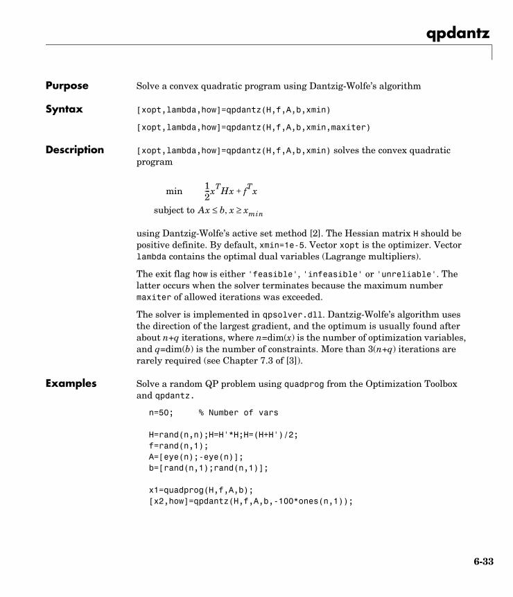
qpdantz
6qpdantzPurpose Solve a convex quadratic program using Dantzig-Wolfe’s algorithm
Syntax [xopt,lambda,how]=qpdantz(H,f,A,b,xmin)
[xopt,lambda,how]=qpdantz(H,f,A,b,xmin,maxiter)
Description [xopt,lambda,how]=qpdantz(H,f,A,b,xmin) solves the convex quadratic program
using Dantzig-Wolfe’s active set method [2]. The Hessian matrix H should be positive definite. By default, xmin=1e-5. Vector xopt is the optimizer. Vector lambda contains the optimal dual variables (Lagrange multipliers).
The exit flag how is either 'feasible', 'infeasible' or 'unreliable'. The latter occurs when the solver terminates because the maximum number maxiter of allowed iterations was exceeded.
The solver is implemented in qpsolver.dll. Dantzig-Wolfe’s algorithm uses the direction of the largest gradient, and the optimum is usually found after about n+q iterations, where n=dim(x) is the number of optimization variables, and q=dim(b) is the number of constraints. More than 3(n+q) iterations are rarely required (see Chapter 7.3 of [3]).
Examples Solve a random QP problem using quadprog from the Optimization Toolbox and qpdantz.
n=50; % Number of vars
H=rand(n,n);H=H'*H;H=(H+H')/2;f=rand(n,1);A=[eye(n);-eye(n)];b=[rand(n,1);rand(n,1)];
x1=quadprog(H,f,A,b);[x2,how]=qpdantz(H,f,A,b,-100*ones(n,1));
min 12---xTHx fTx+
subject to Ax b x xmin≥,≤
6-33

qpdantz
References [2] Fletcher, R. Practical Methods of Optimization, John Wiley & Sons, Chichester, UK, 1987.
[3] Dantzig, G.B. Linear Programming and Extensions, Princeton University Press, Princeton, 1963.
6-34

set
6setPurpose Set or modify MPC object properties
Syntax set(sys,'Property',Value)set(sys,'Property1',Value1,'Property2',Value2,...)set(sys,'Property')set(sys)
Description The set function is used to set or modify the properties of an MPC controller (see “MPC Controller Object” on page 8-2 for background on MPC properties). Like its Handle Graphics counterpart, set uses property name/property value pairs to update property values.
set(MPCobj,'Property',Value) assigns the value Value to the property of the MPC controller MPCobj specified by the string 'Property'. This string can be the full property name (for example, 'UserData') or any unambiguous case-insensitive abbreviation (for example, 'user').
set(MPCobj,'Property1',Value1,'Property2',Value2,...) sets multiple property values with a single statement. Each property name/property value pair updates one particular property.
set(MPCobj,'Property') displays admissible values for the property specified by 'Property'. See “MPC Controller Object” on page 8-2 for an overview of legitimate MPC property values.
set(sys) displays all assignable properties of sys and their admissible values.
See Also mpc, get
6-35
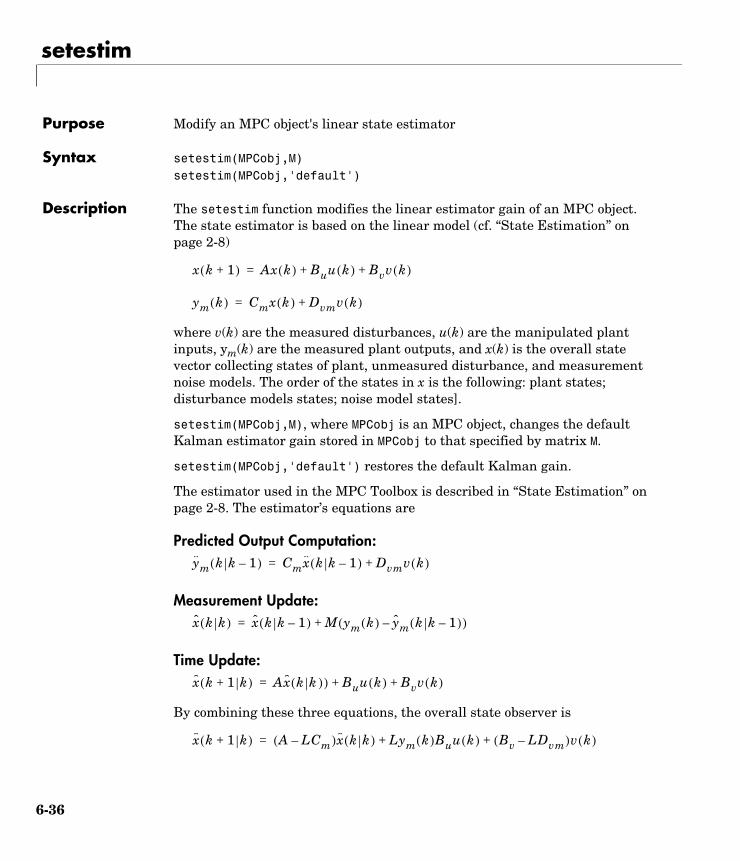
setestim
6setestimPurpose Modify an MPC object's linear state estimator
Syntax setestim(MPCobj,M)setestim(MPCobj,'default')
Description The setestim function modifies the linear estimator gain of an MPC object. The state estimator is based on the linear model (cf. “State Estimation” on page 2-8)
where v(k) are the measured disturbances, u(k) are the manipulated plant inputs, ym(k) are the measured plant outputs, and x(k) is the overall state vector collecting states of plant, unmeasured disturbance, and measurement noise models. The order of the states in x is the following: plant states; disturbance models states; noise model states].
setestim(MPCobj,M), where MPCobj is an MPC object, changes the default Kalman estimator gain stored in MPCobj to that specified by matrix M.
setestim(MPCobj,'default') restores the default Kalman gain.
The estimator used in the MPC Toolbox is described in “State Estimation” on page 2-8. The estimator’s equations are
Predicted Output Computation:
Measurement Update:
Time Update:
By combining these three equations, the overall state observer is
x k 1+( ) Ax k( ) Buu k( ) Bvv k( )++=
ym k( ) Cmx k( ) Dvmv k( )+=
ym k k 1–( ) Cmx k k 1–( ) Dvmv k( )+=
x k k( ) x k k 1–( ) M ym k( ) ym k k 1–( )–( )+=
x k 1 k+( ) Ax k k )( ) Buu k( ) Bvv k( )++=
x k 1 k+( ) A LCm–( )x k k( ) Lym k( )Buu k( ) Bv LDvm–( )v k( )++=
6-36

setestim
where L=AM.
Note The estimator gain M has the same meaning as the gain M in function DKALMAN of the Control Systems Toolbox.
Matrices A, Bu, Bv, Cm, Dvm can be retrieved using getestim as follows:
[M,A,Cm,Bu,Bv,Dvm]=getestim(MPCobj)
As an alternative they can be retrieved from the internal structure MPCobj.MPCData.MPCstruct under the fields A,Bu,Bv,Cm,Dvm (see getmpcdata on page 6-15).
Examples To design an estimator by pole placement, you can use the commands
[M,A,Cm]=getestim(MPCobj);L=place(A',Cm',observer_poles)';M=A\L;setestim(MPCobj,M);
assuming that the linear system AM=L is solvable.
Note The pair (A,Cm) describing the overall state-space realization of the combination of plant and disturbance models must be observable for the state estimation design to succeed. Observability is checked in the MPC Toolbox at two levels: (1) observability of the plant model is checked at construction of the MPC object, provided that the model of the plant is given in state-space form; (2) observability of the overall extended model is checked at initialization of the MPC object, after all models have been converted to discrete-time, delay-free, state-space form and combined together (see the note on page 2-11)
See Also getestim, mpc, mpcstate
6-37

setindist
6setindistPurpose Modify the unmeasured input disturbance model
Syntax setindist(MPCobj,'integrators')setindist(MPCobj,'model,model)
Description setindist(MPCobj,'integrators') imposes the default disturbance model for unmeasured inputs, that is for each unmeasured input disturbance channel, an integrator is added unless there is a violation of observability, otherwise the input is treated as white noise with unit variance (this is equivalent to MPCobj.Model.Disturbance=[])
setindist(MPCobj,'model',model) sets the input disturbance model to model (this is equivalent to MPCobj.Model.Disturbance=model).
See Also mpc, getindist, setestim, getestim, setoutdist
6-38

setmpcdata
6setmpcdataPurpose Set private MPC data structure
Syntax setmpcdata(MPCobj,mpcdata)
Description setmpcdata(MPCobj,mpcdata) changes the private field MPCData of the MPC object MPCobj, where all internal QP matrices, models, estimator gains are stored at initalization of the object. You may only need this for very advanced use of the MPC Toolbox.
Note Changes to the data structure may easily lead to unpredictable results.
See Also getmpcdata, set, get, pack
6-39

setmpcsignals
6setmpcsignalsPurpose Set signal types in MPC plant model
Syntax P=setmpcsignals(P,SignalType1,Channels1,SignalType2,Channels2,...)
Description The purpose of setmpcsignals is to set I/O channels of the MPC plant model P. P must be an LTI object. Valid signal types, their abbreviations, and the channel type they refer to are listed below.
Unambiguous abbreviations of signal types are also accepted.
P=setmpcsignals(P) sets channel assignments to default, namely all inputs are manipulated variables (MVs), all outputs are measured outputs (MOs).More generally, input signals that are not explicitly assigned are assumed to be MVs, while unassigned output signals are considered as MOs.
Examples We want to define an MPC object based on the LTI discrete-time plant model sys with four inputs and three outputs. The first and second input are measured disturbances, the third input is an unmeasured disturbance, the fourth input is a manipulated variable (default), the second output is an unmeasured, all other outputs are measured
sys=setmpcsignals(sys,'MD',[1 2],'UD',[3],'UO',[2]);mpc1=mpc(sys);
Signal Type Abbreviation Channel
Manipulated MV Input
MeasuredDisturbances MD Input
UnmeasuredDisturbances UD Input
MeasuredOutputs MO Output
UnmeasuredOutputs UO Output
6-40

setmpcsignals
Note When using setmpcsignals to modify an existing MPC object, be sure that the fields Weights, MV, OV, DV, Model.Noise, and Model.Disturbance are consistent with the new I/O signal types.
See Also mpc, set
6-41

setname
6setnamePurpose Set I/O signal names in MPC prediction model
Syntax setname(MPCobj,'input',I,name)setname(MPCobj,'output',I,name)
Description setname(MPCobj,'input',I,name) changes the name of the I-th input signal to name. This is equivalent to MPCobj.Model.Plant.InputName{I}=name. Note that setname also updates the read-only Name fields of MPCobj.DisturbanceVariables and MPCobj.ManipulatedVariables.
setname(MPCobj,'output',I,name) changes the name of the I-th output signal to name. This is equivalent to MPCobj.Model.Plant.OutputName{I} =name. Note that setname also updates the read-only Name field of MPCobj.OutputVariables.
Note The Name properties of ManipulatedVariables, OutputVariables, and DisturbanceVariables are read-only. You must use setname to assign signal names, or equivalently modify the Model.Plant.InputName and Model.Plant.OutputName properties of the MPC object.
See Also getname, mpc, set
6-42

setoutdist
6setoutdistPurpose Modify the unmeasured output disturbance model
Syntax setoutdist(MPCobj,'integrators')setoutdist(MPCobj,'remove',channels)setoutdist(MPCobj,'model',model)
Description setoutdist(MPCobj,'integrators') specifies the default method output disturbance model, based on the specs stored in MPCobj.OutputVariables.Integrator and MPCobj.Weights.OutputVariables. Output integrators are added according to the following rule:
1 Outputs are ordered by decreasing output weight (in case of time-varying weights, the sum of the absolute values over time is considered for each output channel. In case of equal output weight, the order within the output vector is followed);
2 By following such order, an output integrator is added per measured outputs, unless (a) there is a violation of observability; (b) The corresponding value in MPCobj.OutputVariables.Integrator is zero; (c) the corresponding weight is zero. A warning message is given when an integrator is added on an unmeasured output channel.
setoutdist(MPCobj,'remove',channels) removes integrators from the output channels specified in vector channels. This corresponds to setting MPCobj.OutputVariables(channels).Integrator=0. The default for channels is (1:ny), where ny is the total number of outputs, that is, all output integrators are removed.
setoutdist(MPCobj,'model',model) replaces the array of output integrators designed by default according to MPCobj.OutputVariables.Integrator with the LTI model model. The model must have ny outputs. If no model is specified, then the default model based on the specs stored in MPCobj.OutputVariables.Integrator and MPCobj.Weights.OutputVariables is used (same as setoutdist(MPCobj, 'integrators').
See Also mpc, getestim, setestim, setoutdist, setindist
6-43
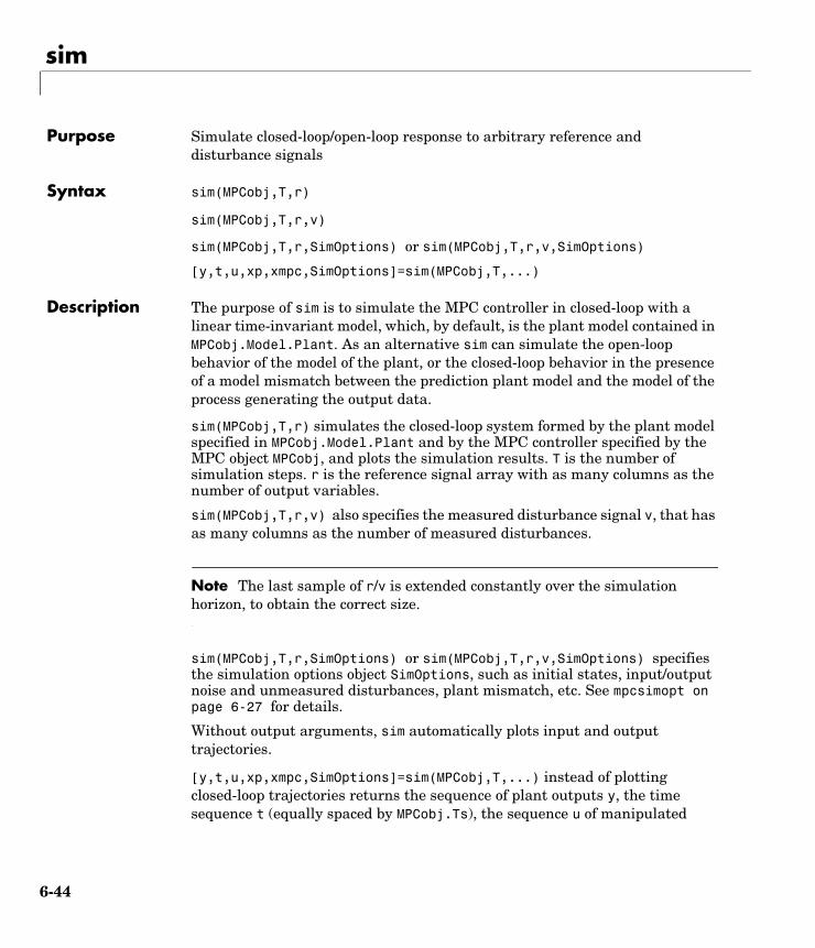
sim
6simPurpose Simulate closed-loop/open-loop response to arbitrary reference and disturbance signals
Syntax sim(MPCobj,T,r)
sim(MPCobj,T,r,v)
sim(MPCobj,T,r,SimOptions) or sim(MPCobj,T,r,v,SimOptions)
[y,t,u,xp,xmpc,SimOptions]=sim(MPCobj,T,...)
Description The purpose of sim is to simulate the MPC controller in closed-loop with a linear time-invariant model, which, by default, is the plant model contained in MPCobj.Model.Plant. As an alternative sim can simulate the open-loop behavior of the model of the plant, or the closed-loop behavior in the presence of a model mismatch between the prediction plant model and the model of the process generating the output data.
sim(MPCobj,T,r) simulates the closed-loop system formed by the plant model specified in MPCobj.Model.Plant and by the MPC controller specified by the MPC object MPCobj, and plots the simulation results. T is the number of simulation steps. r is the reference signal array with as many columns as the number of output variables.
sim(MPCobj,T,r,v) also specifies the measured disturbance signal v, that has as many columns as the number of measured disturbances.
Note The last sample of r/v is extended constantly over the simulation horizon, to obtain the correct size.
sim(MPCobj,T,r,SimOptions) or sim(MPCobj,T,r,v,SimOptions) specifies the simulation options object SimOptions, such as initial states, input/output noise and unmeasured disturbances, plant mismatch, etc. See mpcsimopt on page 6-27 for details.
Without output arguments, sim automatically plots input and output trajectories.
[y,t,u,xp,xmpc,SimOptions]=sim(MPCobj,T,...) instead of plotting closed-loop trajectories returns the sequence of plant outputs y, the time sequence t (equally spaced by MPCobj.Ts), the sequence u of manipulated
6-44

sim
variables generated by the MPC controller, the sequence xp of states of the model of the plant used for simulation, the sequence xmpc of states of the MPC controller (provided by the state observer), and the options object SimOptions used for the simulation.
The descriptions of the input arguments and their default values are shown in the table below.
r is an array with as many columns as outputs, v is an array with as many columns as measured disturbances. The last sample of r/v/d/n is extended constantly over the horizon, to obtain the correct size.
The output arguments of sim are detailed below.
Input Argument Description Default
MPCobj MPC object specifying the parameters of the MPC control law
None
T Number of simulation steps Largest row-size of r,v,d,n
r Reference signal MPCobj.Model.Nominal.Y
v Measured disturbance signal Entries from MPCobj.Model.Nominal.U
SimOptions Object of class @mpcsimopt containing the simulation parameters (See )
[]
Output Argument Description
y Sequence of controlled plant outputs (without noise added on measured ones)
t Time sequence (equally spaced by MPCobj.Ts)
6-45

sim
Examples We want to simulate the MPC control of a multi-input single-output system (the same model as in demo misosim.m). The system has one manipulated variable, one measured disturbance, one unmeasured disturbance, and one output.
%Plant model and initial statesys=ss(tf({1,1,1},{[1 .5 1],[1 1],[.7 .5 1]}));
% MPC object setupTs=.2; % sampling timesysd=c2d(sys,Ts); % prediction model
% Define type of input signalssysd=setmpcsignals(model,'MV',1,'MD',2,'UD',3);
MPCobj=mpc(sysd); % Default weights and horizons
% Define constraints on manipulated variableMPCobj.MV=struct('Min',0,'Max',1);
Tstop=30; % Simulation time
Tf=round(Tstop/Ts); % Number of simulation stepsr=ones(Tf,1); % Reference trajectoryv=[zeros(Tf/3,1);ones(2*Tf/3,1)]; % Measured dist. trajectorysim(MPCobj,Tf,r,v);
See Also mpcsimopt, mpc, mpcmove
u Sequence of manipulated variables generated by MPC
xp Sequence of states of plant model (from Model or SimOptions.Model)
xmpc Sequence of states of MPC controller (estimates of the extended state) This is a structure with the same fields as the mpcstate object.
Output Argument Description
6-46

size
6sizePurpose Display model output/input/disturbance dimensions
Syntax sizes=size(MPCobj)
Description sizes=size(MPCobj) returns the row vector sizes = [nym nu nyu nv nd] associated with the MPC object MPCobj, where nym is the number of measured controlled outputs, nu is the number of manipulated inputs, nyu is the number of unmeasured controlled outputs, nv is the number of measured disturbances, and nd is the number of unmeasured disturbances.
size(MPCobj) by itself makes a nice display.
See Also mpc, set
6-47

ss
6ssPurpose Convert unconstrained MPC controller to state-space linear form
Syntax sys=ss(MPCobj)[sys,Br,Dr,Bv,Dv,Boff,Doff,But,Dut]=ss(MPCobj)[sys,Br,Dr,Bv,Dv,Boff,Doff,But,Dut]=ss(MPCobj,ref_preview,md_previ
ew,name_flag)
Description The ss utility returns the linear controller sys as an LTI system in ss form corresponding to the MPC controller MPCobj when the constraints are not active. The purpose is to use the linear equivalent control in the Control System Toolbox for sensitivity analysis and other linear analysis.
sys=ss(MPCobj) returns the linear discrete-time dynamic controller sys
where ym is the vector of measured outputs of the plant, and u is the vector of manipulated variables. The sampling time of controller sys is MPCobj.Ts.
[sys,Br,Dr,Bv,Dv,Boff,Doff,But,Dut]=ss(MPCobj) returns the linearized MPC controller in its full version, that has the following structure
Note vector x includes the states of the observer (plant+disturbance+noise model states) and the previous manipulated variable u(k-1).
In the general case of nonzero offsets, ym (as well as r, v, utarget) must be interpreted as the difference between the vector and the corresponding offset. Vectors Boff, Doff are constant terms due to nonzero offsets, in particular they are nonzero if and only if MPCobj.Model.Nominal.DX is nonzero (continuous-time prediction models), or MPCobj.Model.Nominal.Dx-MPCobj.Model.Nominal.X is nonzero
x k 1+( ) Ax k( ) Bym k( )+=
u k( ) Cx k( ) Dym k( )+=
x k 1+( ) Ax k( ) Bym k( ) Brr k( ) Bvv k( ) Bututarget k( ) Boff+ + + + +=
u k( ) Cx k( ) Dym k( ) Drr k( ) Dvv k( ) Dututarget k( ) Doff+ + + + +=
6-48

ss
(discrete-time prediction models). Note that when Nominal.X is an equilibrium state, Boff, Doff are zero.
Only the following fields of MPCobj are used when computing the state-space model: Model, PredictionHorizon, ControlHorizon, Ts, Weights.
[sys,...]=ss(MPCobj,ref_preview,md_preview,name_flag) allows you to specify if the MPC controller has preview actions on the reference and measured disturbance signals. If the flag ref_preview='on', then matrices Br and Dr multiply the whole reference sequence:
Similarly if the flag md_preview='on', then matrices Br and Dr multiply the whole measured disturbance sequence:
The optional input argument name_flag='names' adds state, input, and output names to the created LTI object.
Examples To get the transfer function LTIcon from (ym,r) to u,
[sys,Br,Dr]=ss(MPCobj);set(sys,'B',[sys.B,Br],'D',[sys.D,Dr]);
See Also mpc, set, tf, zpk
x k 1+( ) Ax k( ) Bym k( ) Br r k( ) r k 1+( ) … r k p 1–+( );;;[ ] …+ + +=
u k( ) Cx k( ) Dym k( ) Dr r k( ) r k 1+( ) … r k p 1–+( );;;[ ] …+ + +=
x k 1+( ) Ax k( ) … Bv v k( ) v k 1+( ) … v k p+( );;;[ ] …+ + +=
u k( ) Cx k( ) … Dv v k( ) v k 1+( ) … v k p+( );;;[ ] …+ + +=
6-49

tf
6tfPurpose Convert unconstrained MPC controller to linear transfer function
Syntax sys=tf(MPCobj)
Description The tf function computes the transfer function of the linear controller ss(MPCobj) as an LTI system in tf form corresponding to the MPC controller when the constraints are not active. The purpose is to use the linear equivalent control in the Control Systems Toolbox for sensitivity and other linear analysis.
See Also ss, zpk
6-50

trim
6trimPurpose Compute the steady-state value of the MPC controller state for given inputs and outputs values
Syntax x=trim(MPCobj,y,u)
Description The trim function finds a steady-state value for the plant state vector such that x=Ax+Bu, y=Cx+Du, or the best approximation of such an x in a least squares sense, sets noise and disturbance model states at zero, and forms the extended state vector.
See Also mpc, mpcstate
6-51

zpk
6zpkPurpose Convert unconstrained MPC controller to zero/pole/gain form
Syntax sys=zpk(MPCobj)
Description The zpk function computes the zero-pole-gain form of the linear controller ss(MPCobj) as an LTI system in zpk form corresponding to the MPC controller when the constraints are not active. The purpose is to use the linear equivalent control in the Control Systems Toolbox for sensitivity and other linear analysis.
See Also ss, tf
6-52
7
Block Reference
Blocks — Alphabetical List (p. -2) A list of available blocks, sorted alphabetically

7
7-2
Blocks — Alphabetical List 7
This section contains function reference pages listed alphabetically.

MPC Controller Block
7MPC Controller BlockPurpose Compute the MPC control law
Library MPC Simulink Library
Description The MPC Controller Block receives the current measured output, reference signal, and measured disturbance signal, and outputs the optimal manipulated variables by solving a quadratic program. The block is based on an MPC object, which provides performance and constraint specifications, as well as the sampling time of the block.
Dialog Box
Figure 7-1: MPC Controller Block Mask
7-3
MPC Controller Block
MPC controllerMPC controller object, definining prediction model, weights, constraints, sampling time, etc.
Initial controller stateInitial state of the MPC controller. This must be a valid mpcstate object.
Reference signalChoose whether the reference signal is loaded from the workspace or received from the block input port. If the signal is received from the workspace, the checkbox Look Ahead is enabled, and anticipative action can be selected (see “Look Ahead and Signals from the Workspace” at page page 3-4)
Measured disturbanceChoose whether the disturbance signal is loaded from the workspace or received from the block input port. If the signal is received from the workspace, the checkbox Look Ahead is enabled, and anticipative action can be selected (see “Look Ahead and Signals from the Workspace” at page page 3-4)
The mask requires that you specify a valid MPC controller object. There are two ways of providing an MPC controller object:
1 Load an existing MPC object from the workspace, or
2 Push the Design button to open the MPC Design Tool and design the MPC controller object there. Closed-loop simulations can be run while the MPC controller is edited in the MPC Design Tool. In this case, the controller parameters used for simulating the Simulink diagram are those specified in the MPC Design Tool, so that the parameters of the controller can be more easily tuned.
In the latter case, the designed controller must be exported as an MPC object to the workspace when the Tool is closed, so that the new changes can be still used for simulation.
When no MPC controller is specified in the edit box, the Design button will attempt at constructing a default MPC controller by automatically getting a linearized model from the Simulink diagram.
7-4

MPC Controller Block
The checkbox Enable input port for measured disturbance is used to resize the block. If the checkbox is not checked, the block has two input signal, namely measured outputs and references. When the checkbox is checked, the block has measured disturbances has third input signal.
See Also mpc, mpcstate
7-5

MPC Controller Block
7-6

8
Object Reference
This chapter provides reference material for the objects used with the command-line functions. Descriptions of the object properties and fields are given in the following sections.
MPC Controller Object (p. 8-2) Description of the MPC object containing the parameters defining the MPC control law (prediction horizon, weights, constraints, etc.).
MPC State Object (p. 8-13) Description of the MPC object containing the state of an MPC controller.
MPC Simulation Options Object (p. 8-14)
Description of the MPC object containing options for simulating MPC controllers.
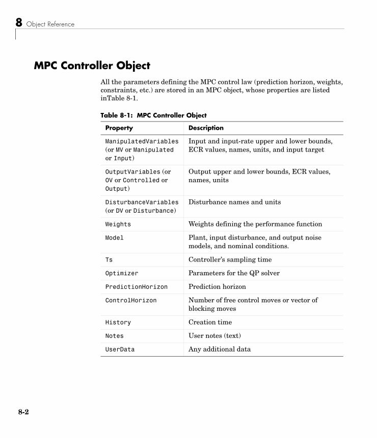
8 Object Reference
8-2
MPC Controller ObjectAll the parameters defining the MPC control law (prediction horizon, weights, constraints, etc.) are stored in an MPC object, whose properties are listed inTable 8-1.
Table 8-1: MPC Controller Object
Property Description
ManipulatedVariables (or MV or Manipulated or Input)
Input and input-rate upper and lower bounds, ECR values, names, units, and input target
OutputVariables (or OV or Controlled or Output)
Output upper and lower bounds, ECR values, names, units
DisturbanceVariables (or DV or Disturbance)
Disturbance names and units
Weights Weights defining the performance function
Model Plant, input disturbance, and output noise models, and nominal conditions.
Ts Controller’s sampling time
Optimizer Parameters for the QP solver
PredictionHorizon Prediction horizon
ControlHorizon Number of free control moves or vector of blocking moves
History Creation time
Notes User notes (text)
UserData Any additional data
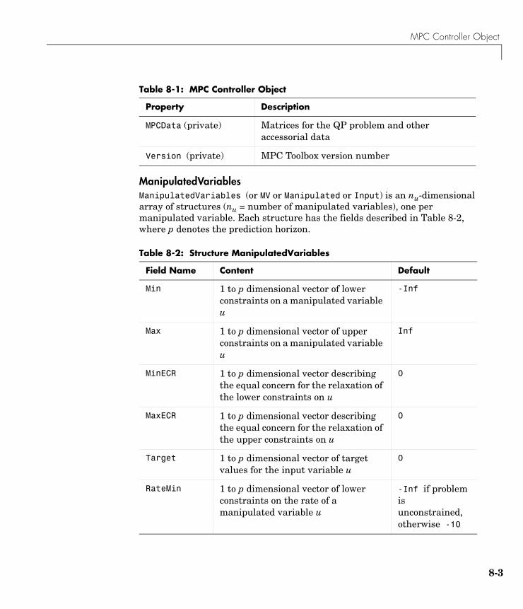
MPC Controller Object
ManipulatedVariablesManipulatedVariables (or MV or Manipulated or Input) is an nu-dimensional array of structures (nu = number of manipulated variables), one per manipulated variable. Each structure has the fields described in Table 8-2, where p denotes the prediction horizon.
MPCData (private) Matrices for the QP problem and other accessorial data
Version (private) MPC Toolbox version number
Table 8-2: Structure ManipulatedVariables
Field Name Content Default
Min 1 to p dimensional vector of lower constraints on a manipulated variable u
-Inf
Max 1 to p dimensional vector of upper constraints on a manipulated variable u
Inf
MinECR 1 to p dimensional vector describing the equal concern for the relaxation of the lower constraints on u
0
MaxECR 1 to p dimensional vector describing the equal concern for the relaxation of the upper constraints on u
0
Target 1 to p dimensional vector of target values for the input variable u
0
RateMin 1 to p dimensional vector of lower constraints on the rate of a manipulated variable u
-Inf if problem is unconstrained, otherwise -10
Table 8-1: MPC Controller Object
Property Description
8-3

8 Object Reference
8-4
Note Rates refer to the difference ∆u(k)=u(k)-u(k-1). Constraints and weights based on derivatives du/dt of continuous-time input signals must be properly reformulated for the discrete-time difference ∆u(k), using the approximation du/dt ≅ ∆u(k)/Ts.
RateMax 1 to p dimensional vector of upper constraints on the rate of a manipulated variable u
Inf
RateMinECR 1 to p dimensional vector describing the equal concern for the relaxation of the lower constraints on the rate of u
0
RateMaxECR 1 to p dimensional vector describing the equal concern for the relaxation of the upper constraints on the rate of u
0
Name Name of input signal. This is inherited from InputName of the LTI plant model
InputName of LTI plant model
Units String specifying the measurement units for the manipulated variable
' '
Table 8-2: Structure ManipulatedVariables
Field Name Content Default

MPC Controller Object
OutputVariablesOutputVariables (or OV or Controlled or Output) is an ny-dimensional array of structures (ny = number of outputs), one per output signal. Each structure has the fields described in Table 8-3, where p denotes the prediction horizon.
In order to reject constant disturbances due for instance to gain nonlinearities, the default output disturbance model used in the MPC Toolbox is a collection of integrators driven by white noise on measured outputs (see “Output Disturbance Model” on page 2-9). Output integrators are added according to the following rule:
1 Measured outputs are ordered by decreasing output weight (in case of time-varying weights, the sum of the absolute values over time is considered
Table 8-3: Structure OutputVariables
Field Name Content Default
Min 1 to p dimensional vector of lower constraints on an output y
-Inf
Max 1 to p dimensional vector of upper constraints on an output y
Inf
MinECR 1 to p dimensional vector describing the equal concern for the relaxation of the lower constraints on an output y
1
MaxECR 1 to p dimensional vector describing the equal concern for the relaxation of the upper constraints on an output y
1
Name Name of output signal. This is inherited from OutputName of the LTI plant model
OutputName of LTI plant model
Units String specifying the measurement units for the measured output
' '
Integrator Magnitude of integrated white noise on the output channel (0=no integrator)
[]
8-5
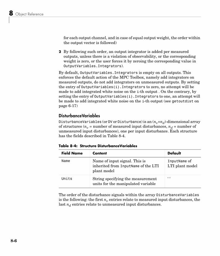
8 Object Reference
8-6
for each output channel, and in case of equal output weight, the order within the output vector is followed)
2 By following such order, an output integrator is added per measured outputs, unless there is a violation of observability, or the corresponding weight is zero, or the user forces it by zeroing the corresponding value in OutputVariables.Integrators).
By default, OutputVariables.Integrators is empty on all outputs. This enforces the default action of the MPC Toolbox, namely add integrators on measured outputs, do not add integrators on unmeasured outputs. By setting the entry of OutputVariables(i).Integrators to zero, no attempt will be made to add integrated white noise on the i-th output . On the contrary, by setting the entry of OutputVariables(i).Integrators to one, an attempt will be made to add integrated white noise on the i-th output (see getoutdist on page 6-17)
DisturbanceVariablesDisturbanceVariables (or DV or Disturbance) is an (nv+nd)-dimensional array of structures (nv = number of measured input disturbances, nd = number of unmeasured input disturbances), one per input disturbance. Each structure has the fields described in Table 8-4.
The order of the disturbance signals within the array DisturbanceVariables is the following: the first nv entries relate to measured input disturbances, the last nd entries relate to unmeasured input disturbances.
Table 8-4: Structure DisturbanceVariables
Field Name Content Default
Name Name of input signal. This is inherited from InputName of the LTI plant model
InputName of LTI plant model
Units String specifying the measurement units for the manipulated variable
' '

MPC Controller Object
Note The Name properties of ManipulatedVariables, OutputVariables, and DisturbanceVariables are read-only. You can set signal names in the Model.Plant.InputName and Model.Plant.OutputName properties of the MPC object, for instance by using the method setname.
WeightsWeights is the structure defining the weighting matrices. Unlike the InputSpecs and OutputSpecs that are arrays of structures, weights is a single structure, whose fields are described in Table 8-5, where p denotes the prediction horizon, nu the number of manipulated variables, ny the number of output variables.
Table 8-5: Structure Weights
Field Name Content Default
ManipulatedVariables (or MV or Manipulated or Input)
nu-by-(1 to p) dimensional array of input weights
zeros(nu,1)
ManipulatedVariablesRate (or MVRate or ManipulatedRate or InputRate)
nu-by-(1 to p) dimensional array of input-rate weights
0.1*ones(nu,1)
OutputVariables (or OV or Controlled or Output)
ny-by-(1 to p) dimensional array of output weights
1 (The default for output weights is the following: if nu>=ny, all outputs are weighted with unit weight; if nu<ny, nu outputs are weighted with unit weight (with a preference on measured outputs), while the remaining outputs are not weighted.)
ECR Weight on the slack variable ε used for softening the constraints
1e5*(max weight)
8-7

8 Object Reference
8-8
ManipulatedVariables, ManipulatedVariablesRate, and OutputVariables are arrays with as many columns as inputs or outputs. If weights are time invariant, then ManipulatedVariables, ManipulatedVariablesRate, and OutputVariables are row vectors, while for time-varying weights, they are an array with up to p rows. The last row is repeated by default in case the matrix has a number of rows smaller than the prediction horizon p.
The default ECR weight is 105 times the largest weight specified in ManipulatedVariables, ManipulatedVariablesRate, and OutputVariables.
Note All weights must be greater than or equal to zero. If all weights on manipulated variable increments are strictly positive, the resulting QP problem is always strictly convex. If some of those weights are zero, the Hessian matrix of the QP problem may become only positive semidefinite. In order to keep the QP problem always strictly convex, if the condition number of the Hessian matrix K∆U is larger than 1012, the quantity 10*sqrt(eps) is added on each diagonal term. This may only occur when all input rates are not weighted (W∆u=0) (see note on page 2-16)
ModelThe property Model specifies plant, input disturbance, and output noise models, and nominal conditions, according to the model setup described in Figure 2-2. It is specified through a structure containing the fields reported in Table 8-6.
Table 8-6: Structure Model Describing the Models Used by MPC
Field Name Content Default
Plant LTI model (or IDMODEL) of the plant
No default
Disturbance LTI model describing color of input disturbances
An integrator on each Unmeasured input channel

MPC Controller Object
Note Direct feedthrough from manipulated variables to measured outputs in Model.Plant is not allowed. See note on page 2-3.
The type of input and output signals is assigned either through the InputGroup and OutputGroup properties of Model.Plant, or, more conveniently, through function setmpcsignals, according to the nomenclature described in Table 8-7 and Table 8-8.
Noise LTI model describing color of plant output measurement noise
Unit white noise on each measured output = identity static gain
Nominal Structure containing the state, input, and output values where Model.Plant is linearized
See Table 8-9
Table 8-7: Input Groups in Plant Model
Name Value
ManipulatedVariables (or MV or Manipulated or Input)
Indices of manipulated variables
MeasuredDisturbances (or MD or Measured)
Indices of measured disturbances
UnmeasuredDisturbances (or UD or Unmeasured)
Indices of unmeasured disturbances
Table 8-6: Structure Model Describing the Models Used by MPC
Field Name Content Default
8-9

8 Object Reference
8-1
By default, all inputs are manipulated variables, and all outputs are measured.
Note With this current release, the InputGroup and OutputGroup properties of LTI objects are defined as structures, rather than cell arrays (see the Control System Toolbox documentation for more details).
The structure Nominal contains the nominal values for states, inputs, outputs and state derivatives/differences at the operating point where Model.Plant was linearized. The fields are reported in Table 8-9 (see “Offsets” on page 2-4).
Table 8-8: Output Groups in Plant Model
Name Value
MeasuredOutputs (or MO or Measured)
Indices of measured outputs
UnmeasuredOutputs (or UO or Unmeasured)
Indices of unmeasured outputs
Table 8-9: Nominal Values at Operating Point
Field Description Default
X Plant state at operating point 0
U Plant input at operating point, including manipulated variables, measured and unmeasured disturbances
0
Y Plant output at operating point 0
DX For continuous-time models, DX is the state derivative at operating point: DX=f(X,U). For discrete-time models, DX=x(k+1)-x(k)=f(X,U)-X.
0
0

MPC Controller Object
TsSampling time of the MPC controller. By default, if Model.Plant is a discrete-time model, Ts=Model.Plant.ts. For continuous-time plant models, you must specify a sampling time for the MPC controller.
OptimizerParameters for the QP optimization. Optimizer is a structure with the fields reported in Table 8-10.
MinOutputECR is a positive scalar used to specify the minimum allowed ECR for output constraints. If values smaller than MinOutputECR are provided in the OutputVariables property of the MPC objects a warning message is issued and the value is raised to MinOutputECR.
PredictionHorizonPredictionHorizon is an integer value expressing the number p of sampling steps of prediction.
ControlHorizonControlHorizon is either a number of free control moves, or a vector of blocking moves (see “Optimization Variables” on page 2-13).
HistoryHistory stores the time the MPC controller was created.
Table 8-10: Optimizer Properties
Field Description Default
MaxIter Maximum number of iterations allowed in the QP solver
200
Trace On/off 'off'Solver QP solver used (only 'ActiveSet') 'ActiveSet'MinOutputECR Minimum positive value allowed for
OutputMinECR and OutputMaxECR1e-10
8-11

8 Object Reference
8-1
NotesNotes stores user’s notes as a cell array of strings.
UserDataAny additional data stored within the MPC controller object
MPCDataMPCData is a private property of the MPC object used for storing intermediate operations, QP matrices, internal flags, etc. See getmpcdata on page 6-15 and setmpcdata on page 6-39.
VersionVersion is a private property indicating the MPC Toolbox version number.
Construction and InitializationAn MPC object is built in two steps. The first step happens at construction of the object when the object constructor mpc is invoked, or properties are changed by a set command. At this first stage, only basic consistency checks are performed, such as dimensions of signals, weights, constraints, etc. The second step happens at initialization of the object, namely when the object is used for the first time by methods such as mpcmove and sim, that require the full computation of the QP matrices and the estimator gain. At this second stage, further checks are performed, such as a test of observability of the overall extended model.
Informative messages are displayed in the command window in both phases, you can turn them on or off using the mpcverbosity command.
2

MPC State Object
MPC State ObjectThe mpcstate object type contains the state of an MPC controller. Its properties are listed in Table 8-11.
The command
mpcstate(mpcobj)
returns a zero extended initial state compatible with the MPC object mpcobj, and with mpcobj.Plant and mpcobj.LastInput initialized at the nominal values specified in mpcobj.Model.Nominal.
Table 8-11: MPC State Object Properties
Property Description
Plant Array of plant states. Values are absolute, i.e., they include possible state offsets (cf. Model.Nominal.X)
Disturbance Array of states of unmeasured disturbance models. This contains the states of the input disturbance model and, appended below, the states of the unmeasured output disturbances model
Noise Array of states of measurement noise model
LastInput Array of previous manipulated variables u(k-1). Values are absolute, i.e., they include possible input offsets (cf. Model.Nominal.U).
8-13

8 Object Reference
8-1
MPC Simulation Options ObjectThe mpcsimopt object type contains various simulation options for simulating an MPC controller with the command sim. Its properties are listed in Table 8-12.
The command
SimOptions=mpcsimopt(mpcobj)
Table 8-12: MPC Simulation Options Properties
Property Description
PlantInitialState Initial state vector of plant model generating the data
ControllerInitialState Initial condition of the MPC controller. This must be a valid @mpcstate object
UnmeasuredDisturbance Unmeasured disturbance signal entering the plant
InputNoise Noise on manipulated variables
OutputNoise Noise on measured outputs
RefLookAhead Preview on reference signal ('on' or 'off')
MDLookAhead Preview on measured disturbance signal ('on' or 'off')
Constraints Use MPC constraints ('on' or 'off')
Model Model used in simulation for generating the data.
StatusBar Display wait bar ('on' or 'off')
MVSignal Sequence of manipulated variables (with offsets) for open-loop simulation (no MPC action)
OpenLoop Performs open-loop simulation
4
MPC Simulation Options Object
returns an empty @mpcsimopt object. You must use set / get to change simulation options.
UnmeasuredDisturbance is an array with as many columns as unmeasured disturbances, InputNoise and MVSignal are arrays with as many columns as manipulated variables, OutputNoise is an array with as many columns as measured outputs. The last sample of the array is extended constantly over the horizon to obtain the correct size.
Note Nonzero values of ControllerInitialState.LastMove are only meaningful if there are constraints on the increments of the manipulated variables.
The property Model is useful for simulating the MPC controller under model mismatch. The LTI object specified in Model can be either a replacement for Model.Plant, or a structure with fields Plant, Nominal. By default, Model is equal to MPCobj.Model (no model mismatch). If Model is specified, then PlantInitialState refers to the initial state of Model.Plant and is defaulted to Model.Nominal.x.
If Model.Nominal is empty, Model.Nominal.U and Model.Nominal.Y are inherited from MPCobj.Model.Nominal. Model.Nominal.X/DX is only inherited if both plants are state-space objects with the same state dimension.
8-15

8 Object Reference
8-1
6
Index
Bblocking
specification 5-36buttons
tool bar 5-6
Cconstraints
hard vs. soft 1-13manipulated variables 5-41optimization problem 2-5output variables 5-42overview 1-7softening 1-13, 5-43specification 5-40, 8-3tolerance band 1-13
Control and Estimation Tools ManagerMPC Design Tool 5-2
control horizon 1-8specification 5-36
control interval 1-5specification 5-36
controller settingsblocking 5-36control interval 5-36estimation 5-50horizons 5-36overall robustness 5-47plant model 5-36
controller specificationsconstraint softening 5-43constraints 5-40relaxation bands 5-43weights 5-47
controllerscopying 5-29
creating 5-29deleting 5-29exporting 5-5, 5-19, 5-29from MAT-file 5-17from workspace 5-16importing 5-4, 5-15, 5-29notes 5-29renaming 5-8specification 5-36summary listing 5-29
Ddata markers 5-67DC gain 6-6delays
horizons for 1-8description
specification 5-22design tool
closing 5-4renaming tree nodes 5-8starting 5-2tree navigation 5-7
disturbance estimationcontroller settings 5-50
disturbancesinput model 6-14inputs 5-54internal state 6-29output model 6-17outputs 5-52simulation specification 5-59type definition 6-40
durationspecification 5-59
Index-1

Index
Ind
Eestimation
controller settings 5-50gain 6-36Kalman filter 2-10model 2-8, 6-11state 1-7, 1-13See also observer
Ffeedforward compensation 1-4file menu
close design tool 5-4load saved design 5-3new design 5-3save current design 5-4
Hhold
zero-order 1-7horizons
control 1-8prediction 1-8
Iidentified models 2-19importing
controller from MAT-file 5-17controller from workspace 5-16controllers 5-15model from MAT-file 5-11model from workspace 5-10
inputsdisturbance model 6-14
ex-2
property specifications 5-23inverse-response 1-8
KKalman filter 2-10
Llinearization
during model import 5-12offset 2-4operating point selection 5-13options 5-13procedure 5-13
load button 5-6
Mmanipulated variables
example 1-3setpoints 1-12
MAT-filecontroller export 5-19controller import 5-17model import 5-11
measured disturbancesexample 1-3
memory 6-8menus
file 5-3menu bar 5-3MPC 5-4
modelscontroller specification 5-36deleting 5-26disturbance 1-5, 5-50

Index
from MAT-file 5-11from workspace 5-10identified 2-19import tool 5-9importing 5-26importing plant model 5-4input disturbance 6-14linearization during import 5-12mismatch 6-27, 8-15noise 5-50notes 5-26output disturbance 2-9, 6-17summary list 5-26viewing details 5-26
movessuppression 1-11
MPC 7-3MPC menu
export 5-5import controller 5-4import plant model 5-4simulation start 5-5
MPC state 6-29MPCTOOL function
starting 5-2
Nnames
specification 5-22new design button 5-6nodes
controller specification 5-7controllers list 5-7MPC project/task 5-7plant models list 5-7renaming 5-8
simulation scenario specification 5-7simulation scenarios list 5-7types 5-7
noisecontroller settings 5-56
nominal conditions 2-4, 8-10nominal values
specification 5-22notes
controllers 5-29models 5-26scenarios 5-33
Oobserver 2-8
gain 6-36initialization 8-12model 6-11See also estimation
offset 8-10linearization 2-4
optimal trajectory 6-21optimization 1-7
setpoint tracking 1-10outputs
disturbance model 2-9, 6-17property specifications 5-24
Pplant model importer 5-9plant/model mismatch
simulation specification 5-59plants
initial state 8-14MIMO 1-10
Index-3

Index
Ind
mismatch 6-27, 8-15nonminimum phase 1-8nonsquare 1-10SISO 1-3state 2-3
plotsdata markers 5-67normalizing 5-71simulation responses 5-67variable selection 5-70
prediction horizon 1-8specification 5-36
projectscontroller import 5-17importing model 5-11load 5-3new 5-2renaming 5-8save 5-4
propertiesoutput signals 5-24signal specifications 5-22
Rrelaxation bands
specification 5-43response plots 5-67
See also plotsrobustness
global setting 5-47
Ssave button 5-6scenarios
comparing 5-69
ex-4
controller option 5-59copying 5-33creating 5-33current 5-5deleting 5-33duration 5-59notes 5-33plant model option 5-59renaming 5-8settings 5-59simulation button 5-59summary list 5-33
setpointsspecification in simulations 5-59
signal definitionoverview graphic 5-22property specification table 5-22specification view 5-21
signal propertiesinputs 5-23specification 5-22
signal typespecification 5-22
signalsdescription 5-22names 5-22nominal values 5-22types 1-4, 5-22units 5-22
simulate button 5-6simulations
closed-loop option 5-59duration 5-59open-loop option 5-59response plots 5-67start using MPC menu 5-5
Simulink

Index
block 7-3initial state 7-4look-ahead 7-4
statecontroller 3-5, 6-29observer 2-8, 2-10
See also estimationstate estimation 1-13states
initial 8-14plant 2-3
steady-state 6-6system identification
model conversion 2-19
Ttasks
importing model 5-11tolerance bands 1-13tool bar
overview 5-6tree view
node types 5-7overview 5-7
Uunconstrained control 6-6units
specification 5-22unmeasured disturbances
example 1-3input model 6-14output model 6-17
Vviews
signal definition 5-21tree 5-7
Wweights
inputs 5-48optimization problem 2-5outputs 5-49specification 5-47, 8-7tuning 5-47
workspacecontroller export 5-19importing model from 5-10
Index-5

Index
Ind
ex-6