Model-Reduced Variational Fluid Simulation

Beibei LiuMSU

Gemma MasonCaltech/U. Auckland

Julian HodgsonUCL

Yiying TongMSU

Mathieu DesbrunCaltech-INRIA

Abstract

We present a model-reduced variational Eulerian integrator for in-compressible fluids, which combines the efficiency gains of di-mension reduction, the qualitative robustness of coarse spatial andtemporal resolutions of geometric integrators, and the simplicity ofsub-grid accurate boundary conditions on regular grids to deal witharbitrarily-shaped domains. At the core of our contributions is afunctional map approach to fluid simulation for which scalar- andvector-valued eigenfunctions of the Laplacian operator can be eas-ily used as reduced bases. Using a variational integrator in time topreserve liveliness and a simple, yet accurate embedding of the fluiddomain onto a Cartesian grid, our model-reduced fluid simulatorcan achieve realistic animations in significantly less computationaltime than full-scale non-dissipative methods but without the numer-ical viscosity from which current reduced methods suffer. We alsodemonstrate the versatility of our approach by showing how it eas-ily extends to magnetohydrodynamics and turbulence modeling in2D, 3D and curved domains.CR Categories: I.3.7 [Computer Graphics]: Three-DimensionalGraphics and Realism—Animation.Keywords: Computational fluid dynamics, model reduction, Eule-rian simulation, energy preservation, sub-grid-resolution geometry.

1 Introduction

Accurate simulation of incompressible fluids is a well-studied topicin computational fluid dynamics. Fluid animation research is drivenby a different emphasis: in the context of computer graphics, thefocus is on capturing the visual complexity of typical incompress-ible fluid motions (such as vortices and volutes) with minimumcomputational cost. However, this relentless quest for efficiencyhas often resulted in time integrators that exhibit large numeri-cal viscosity [Stam 1999], as they proceed via operator splittingthrough advection followed by divergence-free projection. The in-curred numerical dissipation has also, besides its obvious visual ar-tifacts, the unintended consequence that previews on coarse spa-tial and temporal resolutions are far from predictive of the final,high-resolution run. Non-dissipative methods have been proposedmore recently [Mullen et al. 2009]; however, they require large,non-linear solves, hampering efficiency. On the other hand, model-reduced integrators [Treuille et al. 2006] manipulate a smaller setof degrees of freedom found via Galerkin dimension reduction tocapture the main components of the flow efficiently, at the cost ofexcessive vorticity smearing. Similarly, regular spatial grids are of-ten preferred due to their significantly lighter data structures andsparser stencils—yet, their use conflicts with the proper treatmentof boundary conditions over complex, non-grid-aligned domains.

Figure 1: Model-reduced fluids on regular grids. Our energy-preserving approach integrates a fluid flow variationally using asmall number of divergence-free velocity field bases over an arbi-trary domain (visualized here are the 5th, 10th, and 15th eigenvec-tors of the 2-form Laplacian) computed with subgrid accuracy on aregular grid (here, a 42×42×32 grid). Our integrator is versatile:it can be used for realtime fluid animation, magnetohydrodynamics,and turbulence models, with either explicit or implicit integration.

While pressure projection with subgrid accuracy have been recentlyproposed on Cartesian grids [Batty et al. 2007; Ng et al. 2009], non-dissipative methods still require boundary-conforming meshes.

In this paper, we introduce a variational model-reduced Eulerianfluid solver with sub-grid accuracy which bypasses the traditionalnumerical curses of Galerkin projected dynamics, while keepingthe efficiency of Cartesian grid-based simulation.

1.1 Background

Early computer animation Eulerian methods for incompressiblefluid simulation were based on explicit finite differences [Fosterand Metaxas 1997] which suffered from the slow convergence oftheir iterative approach to divergence-free projection. Stam [1999]introduced semi-Lagrangian advection and a sparse Poisson solverwhich brought much improved efficiency and stability. However,these improvements came at the cost of significant dissipation—acommon issue that one can partially mitigate via vorticity confine-ment [Steinhoff and Underhill 1994], reinjection of vorticity withparticles [Selle et al. 2005], or curl correction [Zhang et al. 2015].Significantly less dissipative time integrators were also proposedthrough semi-Lagrangian advection of vorticity [Elcott et al. 2007],or even energy-preserving methods [Mullen et al. 2009]. How-ever, these improved numerical methods often carry higher compu-tational costs. Consequently, coupled Eulerian-Lagrangian (hybrid)methods (see, for instance, [Losasso et al. 2008; Golas et al. 2012])have flourished recently, as they offer a good compromise betweenefficiency and dissipation.

Handling boundaries well is also crucial for incompressible fluids,as boundary layers can significantly impact fluid motion. Avoidingthe staircase effects that voxelized domains generate was achievedusing simplicial meshes or hybrid meshes [Feldman et al. 2005],but irregular connectivity often affects the efficiency of the solversinvolved. Inspired by the immersed boundary and interface meth-ods, the use of regular grids with modified numerical operators tohandle arbitrary domains was proposed in [Batty et al. 2007], thenmade convergent by [Ng et al. 2009] while maintaining symmetryof the solves needed by the integrators. Another approach usingvirtual nodes was also proposed recently [Howes et al. 2013].

Fluid simulation over non-flat domains has received significant

attention as well. Most notably, Stam adapted his Stable Fluidmethod to handle curvilinear coordinates [Stam 2003], while Azen-cot et al. [2014] recently proposed to use the Lie derivative operatorrepresentation in the spectral domain to represent a velocity field onan arbitrary surface, and performed advection of vorticity througha linearized exponential map of the operator representation. Meth-ods that are using only intrinsic operators can also handle curveddomains without alterations [Elcott et al. 2007; Mullen et al. 2009].

While most Eulerian methods use a finite-dimensional descriptionof the fluid using DOFs on cell faces or centers, model reductionwas also introduced in an effort to approximate the fluid motionusing only a small number of basis functions. The early days ofcomputational fluid dynamics for atmospheric simulation proposedto reduce complexity by discarding high frequencies through theuse of a low number of modes (typically, harmonics or spheri-cal harmonics) to describe the vector field [Silberman 1954; Yu-dovich 1963], while pseudo-spectral methods leveraged fast con-version between modal coefficients and spatial representation viathe Fast Fourier Transform for highly symmetric domains [Orszag1969]. Dimensionality reduction was first introduced for fluid ani-mation by Treuille et al. [2006] through Galerkin projection onto areduced set of basis functions computed through principal compo-nent analysis of a training set of fluid motions. Their method wasdemonstrated on regular grids, but is generalizable to tetrahedralmeshes. A number of works followed, proposing the use of dif-ferent bases such as Legendre polynomials [Gupta and Narasimhan2007], trigonometric functions [Long and Reinhard 2009], or evennon-polynomial Galerkin projection [Stanton et al. 2013]; eventu-ally, Laplacian eigenvectors were pointed out by [De Witt et al.2012] to be particularly appropriate harmonics as they guarantee di-vergence free flows and facilitate the conversion between vorticityand velocity, while offering a sparse advection operator for sym-metric domains. These eigenfunctions also allow easy implementa-tion of viscosity, and eliminate the need for training sets of velocityfields. For simulations involving moving solids, model reductioncan also be conducted on a moving grid [Cohen et al. 2010]. Theuse of cubature, initially proposed to achieve model-reduced simu-lation of elastic models [An et al. 2008; von Tycowicz et al. 2013;Li et al. 2014], can speed up re-simulation of fluids in a reducedsubspace as well [Kim and Delaney 2013]. However, the gain inefficiency of all such model-reduced simulations is often counter-balanced by (at times severe) energy or vorticity dissipation and theneed for unstructured meshes to capture complex boundaries.

1.2 Contributions

In this paper, we formulate a model-reduced variational fluid in-tegrator that combines the benefits of non-dissipative integratorswith the use of dimension reduction and Cartesian grids overarbitrary domains. Based on a description of the fluid motionthrough functional maps, a variational integrator is derived fromHamilton’s principle [Marsden and West 2001; Kharevych et al.2006], resulting in a Lie algebra integrator with non-holonomicconstraints [Pavlov et al. 2011; Gawlik et al. 2011]. We use spec-tral approximation of the functional map through (cell-based) scalarand (face-based) vector Laplacian eigenvectors in order to offermodel reduction without losing the variational properties of the in-tegrator, with controllable energy cascading. This setup allows us touse not only low frequencies to capture the basic behavior of a flow,but also a few selected higher frequencies to add realism at low cost.Furthermore, we extend the embedded-boundary approach of [Nget al. 2009] to our framework in order to compute spectral (scalar-and vector-valued) basis functions of arbitrary domains directly onregular grids for fast computations with sub-grid accuracy. Finally,our approach uses the typical Eulerian setup of flux-based solvers;consequently, addition of fine details through spectral noise [Stam

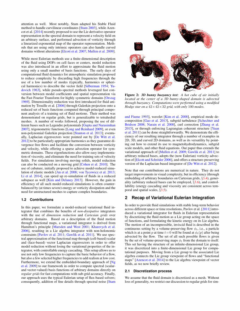
Figure 2: 3D bunny buoyancy test: A hot cube of air initiallylocated at the center of a 3D bunny-shaped domain is advectedthrough buoyancy. Computations were performed using a modifiedHodge star on a 42×42×32 grid, with only 100 modes.

and Fiume 1993], wavelet [Kim et al. 2008], empirical mode de-composition [Gao et al. 2013], subgrid turbulence [Schechter andBridson 2008; Narain et al. 2008], curl correction [Zhang et al.2015], or through enforcing Lagrangian coherent structure [Yuanet al. 2011] can be done straightforwardly. We demonstrate the effi-ciency of our resulting integrator through a number of examples in2D, 3D, and curved 2D domains, as well as its versatility by point-ing out how to extend its use to magnetohydrodynamics, subgridscale models, and other fluid equations. Our paper thus extends thevariational approach of [Mullen et al. 2009; Gawlik et al. 2011] toarbitrary reduced bases, adopts the (now Eulerian) vorticity advec-tion of [Elcott and Schroder 2006], and offers a structure-preservingversion of the Laplacian-based integrator of [De Witt et al. 2012].

Note that our contributions are numerical in nature. They do nottarget improvements in visual complexity, but in efficiency (throughembedding of arbitrary boundaries on Cartesian grids, §3.4), gener-ality (arbitrary reduced bases can be employed, §3.6), and control-lability (energy cascading and viscosity are consistent across tem-poral and spatial scales, §3.5).

2 Recap of Variational Eulerian Integration

In order to provide fluid simulations with stable long-term behavioracross different space or time resolutions, Pavlov et al. [2011] intro-duced a variational integrator for fluids in Eulerian representationby discretizing the fluid motion as a Lie group acting on the spaceof functions, and formulating the kinetic energy on its Lie algebra.The motion of an incompressible, inviscid fluid is described in thecontinuous setting by a volume-preserving flow φt, i.e., a particlewhich is at a point p at time t=0 will be found at φt(p) after beingadvected by the flow. The set of all such possible flows is givenby the set of volume-preserving maps φt from the domain to itself.This set having the structure of an infinite-dimensional Lie group,it was discretized into a finite-dimensional Lie group for compu-tational purposes. Moving from a Lie group to the associated Liealgebra connects the Lie group viewpoint of flows and “functionalmaps” [Azencot et al. 2014] to the Lie algebra viewpoint of vectorfields, as we now briefly review.

2.1 Discretization process

We assume that the fluid domain is discretized as a mesh. Withoutloss of generality, we restrict our discussion to regular grids for sim-

plicity, as we will show in Sec 3.4 how to embed arbitrary domainsinto a Cartesian grid. We discretize a continuous function f(x) onour space by taking an average (integrated) value fi per grid cell i ofthe mesh, which we arrange in a vector f . This definition of discretefunctions allows us to discretize the set of possible flows φt using afunctional map (or Koopman operator) (f φ−1

t )(x)=f(φ−1t (x)).

Specifically, this functional map is encoded as a matrix q of sizethe square of the number of cells, representing the action of φt onany discrete function; that is, the integrated values f of f per cellbecome qf once f is advectedby the flow φ. Because thediscrete flow acts as a func-tional map, it should alwaystake the constant function toitself. That is, for all q, we re-quire that q1 = 1, where 1 isa vector of ones (see [Pavlov et al. 2011] for the equivalent condi-tion on an arbitrary mesh). This is the same as saying that the rowsums of q are equal to 1, i.e., q is signed stochastic. Since we aresimulating an incompressible fluid, we also require that the discreteflow be volume-preserving. This condition is achieved by askingthat the discrete flow preserves the inner product of vectors, thatis, q is orthogonal, i.e., qt = q−1. Thus, we find that we need totake q to be an element of the Lie group G of orthogonal, signedstochastic matrices. This matrix group represents our discrete fluidconfiguration, as we describe next.

2.2 The Eulerian Lie Algebra viewpoint

We can view the finite-dimensional Lie group G as a configurationspace: it encodes the space of possible “positions” for the discretefluid, in that each element of the Lie group represents a possibleway that the fluid could have evolved from its initial position. ThisLie group represents a Lagrangian perspective as it identifies thefluid particles in a given cell by recording which cells they origi-nally came from. The associated Eulerian perspective is given bythe Lie algebra g of matrices of the form q q−1 for q ∈ G. Itwas shown in [Pavlov et al. 2011] that any matrix A∈g of this Liealgebra is both antisymmetric (At = −A) and row-null (A1 = 0),and corresponds to a discrete counterpart of the Lie derivative Lvwith respect to the continuous velocity field v = φ φ−1. Thus,the product Af of such a matrix with a discrete function f approx-imates the continuous term v · ∇f . Furthermore, if cells i and jare nearest neighbors, then the matrix element Aij represents theflux of the fluid through the face shared by cells i and j. Thus, anelement of the Lie algebra g of G is directly linked to the usualflux-based (Marker And Cell) discretization of vector field in fluidsimulators [Harlow and Welch 1965].

2.3 Non-holonomic constraint

Whilst the elements Aij for A ∈ g have a clear physical interpre-tation in the case where i and j are nearest neighbors, this is notthe case for elements representing interactions between cells thatare not immediate neighbors. Similarly to a CFL condition, weprohibit fluid particles from skipping to non-neighboring cells, byrestricting the Lie algebra to the constrained set S, the set of ma-trices A such that Aij = 0 unless cells i and j share a face (or anedge in 2D). We require the elements of g that we use to representthe fluid velocity fields to fall into this constrained set. This has theadditional advantage of making the matrices sparse, dramaticallydecreasing the amount of memory required and the computationaltime, as much fewer degrees of freedom need to be updated—andnow, the traditional MAC discretization with fluxes corresponds ex-actly to a Lie algebra element in this constrained set.

Constraining the matrices in this way requires a non-holonomicconstraint, because the set S is not closed under the Lie bracket.

That is, interactions between nearest neighbors followed by fur-ther interactions between nearest neighbors produce interactionsbetween cells that are two-away from each other, which are there-fore not inside the constrained set S.

2.4 Creating a variational numerical method

Using this discretization, one can create a variational numericalmethod for ideal, incompressible fluids through the Euler-Poincareequations [Gawlik et al. 2011] for the Lagrangian given by

LEuler =1

2〈A,A〉 ≈ 1

2

∫v2 dx, (1)

and subject to the non-holonomic constraint A ∈ S. The result-ing numerical method exhibits no numerical dissipation, and pro-duces good qualitative behavior over long timescales. Changing thetime integration scheme to be time reversible leads to exact energypreservation [Mullen et al. 2009]. With control over dissipationand robustness to time step and grid size, this computational toolgreatly facilitates the design of fluid animation. Note that this vari-ational integrator also guarantees that the relabeling symmetry im-plies a discrete version of Kelvin’s circulation theorem, i.e., circu-lation of velocity field (represented as a Lie algebra element) alonga closed loop (represented as a 1-cycle [Pavlov et al. 2011]) trans-ported along the fluid flow is invariant, which helps keep the vividdetails of vorticity in the fluid simulation without resorting to addi-tional energy-injecting measures such as vorticity confinement, asshown in [Elcott et al. 2007; Mullen et al. 2009]. However, the timeintegration requires a quadratic solve based on all the fluxes in thedomain, making it inappropriate for realtime simulation.

3 Model-reduced Variational Integrator

We present an integrator which extends the approach of [Pavlovet al. 2011], using a different functional-map Lie group, similarlyinterlinked with an Eulerian velocity-based Lie algebra picture. Ourmethod offers the additional advantage of fast computations on ar-bitrary domains: we use reduced coordinates to encode the mostsignificant components of the spatial scalar and vector fields, andperform subgrid accurate precomputations on simple regular grids.We will focus on Euler equations first, before discussing variantssuch as Navier-Stokes and magnetohydrodynamics (MHD).

3.1 Spectral Bases

We first define the discrete, reduced scalar and velocity fields onwhich our functional map Lie group will act. Extending what wasadvocated in [De Witt et al. 2012], we use the orthonormal bases for2-forms and 3-forms given by the eigenfunctions of the deRham-Laplacian operators on an arbitrary discrete mesh M. These arecalculated using the discrete operators of Discrete Exterior Cal-culus [Desbrun et al. 2008; Arnold et al. 2006], allowing us toleverage the large literature on their implementation and structure-preserving properties. From this small set of basis functions, weefficiently encode through reduced coordinates the full-space fieldstypically used in the MAC scheme, i.e., fluxes through cell bound-aries (discrete 2-forms) to represent velocity fields, and densitiesintegrated in each cell (discrete 3-forms) to represent scalar fields(such as smoke density or geostrophic momentum in rotating strat-ified flow [Desbrun et al. 2013]).

Choice of bases. We denote the i-th eigenfunction of the 3-formLaplacian ∆3 as Φi, with associated eigenvalue −µ2

i ,

∆3Φi = −µ2iΦi.

The eigenfunctions corresponding to the M3+1 smallest µi can beassembled into a low-frequency basis

Φ0, ...,ΦM3.

Note that depending on the boundary condition, µ0 = 0 may cor-respond to more than one harmonic function; but these remain sta-tionary when advected by divergence-free velocity fields with zeroflux across the boundary, and are thus omitted in our discussion.

Similarly, we denote the i-th eigenfunction of the 2-form Laplacian∆2 as Ψi, with its associated eigenvalue −κ2

i :

∆2Ψi = −κ2iΨi.

We also assemble the first M2 eigenvector fields (corresponding tothe M2 smallest κi) into a finite dimensional low-frequency basis,

Ψ1, ...ΨM2.Some of the 2-form eigenfunctions are not divergence-free, andthese eigenfunctions can be identified as gradient fields, ∇Φi/µi(see §A). Thus, we can reorder the eigenfunctions of ∆2 into

h1, ..., hβ1 ,∇Φ1

µ1, ...,∇ΦM3

µM3

,Ψ1, ...ΨMC,

where hi are harmonic 2-forms (corresponding to frequency κi=0)with β1 being the first Betti number determined by the topologyof the domain (basically, the number of tunnels plus the numberof connected components of the boundary minus one), and MC =M2−M3−β1 denoting the number of non-harmonic but divergence-free basis functions.

Discretization. Computing our spectral bases requires a proper dis-cretization of the Laplacian operators and of boundary conditions.Both topics are well studied, and many implementations can beleveraged [Elcott and Schroder 2006; Bell and Hirani 2008]. Inparticular, we note that discrete Laplacians are typically integratedLaplacians, meaning that the two eigenvalue problems mentionedabove are discretized as two generalized eigenvalue problems

(?3∆3)Φi=−µ2i ?3 Φi and (?2∆2)Ψi=−κ2

i ?2 Ψi

respectively, to make the discrete operators symmetric and thus al-low for efficient numerical solvers. We provide a detailed guide todiscretization on arbitrary unstructured meshes in §A to explicatehow to enforce no-transfer and free-slip conditions (corresponding,respectively, to vn|∂M= 0 and ∂vt/∂n |∂M= 0 if the continuousvelocity field is decomposed at the boundary into its normal andtangential components, v = vn+vt). Note that only two opera-tors are required: the exterior derivative d and the Hodge star ?.The first operator is purely topological, while the second is just ascaling operation per edge, face, and cell. Moreover, we will seein §3.4 that this latter operator can be trivially modified to handlearbitrary fluid domains without having to use anything else but aregular grid. From these two operators, both Laplacians are easilyassembled, and low-frequency eigenfields are found via Lanczositerations.

3.2 Spectral Lie group

While earlier methods [Pavlov et al. 2011; Gawlik et al. 2011] havedefined scalar fields using a spatial representation through linearcombinations of locally-supported piecewise-constant basis func-tions, we use a spectral representation through linear combinationsof the aforementioned spectral basis functions Φi, allowing us todrastically reduce the number of degrees of freedom the integra-tor will have to update, while still conforming to the shape of thedomain (see Fig. 3).

Lie group. We encode the fluid motion through a time-varying Liegroup element q(t) that represents a functional map induced by thefluid flow φt, mapping a function f(x) =

∑i fiΦi(x) linearly to

another function g(x)=∑i giΦi(x) such that g(x)=f φ−1(x).

As the function space is approximated by a finite dimensional spacespanned by low-frequency basis functions, q can be encoded by a(M3+1)×(M3+1) matrix. The volume-preserving property of the

Figure 3: Effect of shape on spectral bases: The Laplacian eigen-vectors depends heavily on the domain Ω. Here, rectangle (top) vs.ellipse (bottom) domains (both computed on 2D rectangular grid ofsize 602) exhibit very different eigenvectors Ψ10 and Φ10.

flow still implies the orthogonality of the matrix, i.e, qtq= Id. Sowe are looking for a subgroup of O(M3+1), or, more accurately,of SO(M3 +1), since we wish to describe gradual changes fromthe identity. The condition that constant functions are mapped tothemselves in this low-frequency Lie group becomes q0i = δ0i andqi0 = δi0, where δij is the Kronecker symbol, since 0-th frequencyrepresents the constant function. This effectively removes one di-mension, and the Lie group that we are using is thus isomorphic toSO(M3). This is much smaller than the full Lie group used for thespatial representation [Pavlov et al. 2011] which had a dimensionproportional to the square of the number of cells of the mesh—apotential reduction of several orders of magnitude.

Lie algebra. We identify each velocity eigenfunction Ψm with anelement of the Lie algebra of the above Lie group as follows. Wetake the Lie derivative along the velocity field Ψm of a scalar eigen-function Φj , then we project the resulting scalar field onto anotherscalar eigenfunction Φj , producing a matrix Am for each velocityeigenfunction Ψm, with entries

Am,ij =

∫M

Φi(Ψm · ∇Φj). (2)

ComputingAm amounts to turning a 3-form into a dual 0-form firstwith ?3, and then carrying out the integral in the (diamond) volumespanned by each face and its dual edge: this way, the differentialof the dual 0-form from Φj is multiplied by the 2-form Ψm on theface and the average dual 0-form from Φi on the face. Notice thatwe have 〈Am, An〉=δmn by construction thanks to the basis of Ψbeing orthonormal. As in the non-spectral case, the divergence-freecondition leads to the antisymmetry of these matrices since

Am,ij+Am,ji =

∫M

Ψm · ∇(ΦiΦj) = −∫M

ΦiΦj∇ ·Ψm = 0.

This is expected, since the Lie algebra so(M3) of SO(M3) con-tains only antisymmetric matrices. The Lie algebra has a Liebracket operator, which is given by the usual matrix commutator[Am, An]=AmAn −AnAm.

Non-holonomic constraint. Just like in [Pavlov et al. 2011], notevery element of the Lie algebra so(M3) will correspond to a fluidvelocity spanned by the eigenfunctions Ψm. We force the dynam-ics on the Lie algebra to remain within the domain of physically-sensible elements using the following non-holonomic constraint,which keeps the velocity within the space spanned by the lowestfrequency MC+β1 divergence-free 2-form basis fields:

A =

MC+β1∑i=1

vi Ai (3)

where vi is a coefficient for Ai representing the modal amplitudeof frequency κi. This linear condition can thus be seen as an in-tuitive extension of the one-away spatial constraint on Lie algebraelements used in [Pavlov et al. 2011] that we mentioned in §2.3.

3.3 Spectral variational integrator

The Lagrangian of the fluid motion (i.e., its kinetic energy in thecase of Euler fluids) can be written as LEuler = 1

2〈A(t), A(t)〉 as we

reviewed in §2.4. Thus, the equation of motion can be derived fromHamilton’s (least action) principle∫

〈A(t), δA〉dt = 0, (4)

where δA=δ(qq−1) is the variation ofA induced by variation of q.If we denote B≡δqq−1, one has δA=δqq−1−qq−1δqq−1. SinceB= δqq−1−δqq−1qq−1, we find that δA is induced by variationsof q only if it satisfies Lin’s constraints [Gawlik et al. 2011]:

δA = B + [B,A], (5)where B=

∑i biAi is an arbitrary element of the Lie algebra with

coordinates bii in the 2-form basis. Substituting Eq. (5) intoEq. (4), we then have

0 =

∫〈A, δA〉 dt

=

∫ ∑i,k

vibk 〈Ai, Ak〉+∑i,j,k

vivjbk 〈Ai, [Ak, Aj ]〉 dt

=

∫ ∑k

(−∑i

vi 〈Ai, Ak〉+∑i,j

vivj 〈Ai, [Ak, Aj ]〉)bk dt.

Since this last equation must be valid for any bk, the update rule forthe velocity field has to be:vk =

∑i

vi 〈Ai, Ak〉 =∑i,j

vivj 〈Ai, [Ak, Aj ]〉 ≡ vtCkv, (6)

where v is the column vector storing the coefficients vi of the dis-crete velocity A (Eq. (3)), and Ck is the square matrix with

Ck,ij = 〈Ai, [Ak, Aj ]〉 =

∫M

(∇×Ψi) · (Ψk×Ψj). (7)

Note that this velocity update do not even require the scalar (3-form) bases used in the definition of the Lie group; however, thesebases become important in more general simulations, includingmagnetohydrodynamics and rotating stratified flows.

Time integrator. The continuous-time update in Eq. (6) is then dis-cretized via either a midpoint rule (which will lead to an energy-preserving model-reduced variant of [Mullen et al. 2009]) or atrapezoidal rule (which corresponds to a model-reduced variant ofthe variational method of [Pavlov et al. 2011]). Specifically, themidpoint rule is implemented as

vt+hk − vtk = h∑i,j

Ck,ijvti + vt+hi

2

vtj + vt+hj

2, (8)

The energy preservation can be easily verified by multiplyingvtk + vt+hk on both sides of the above equation, summing over k,and invoking the property of coefficients Ck,ij = −Cj,ik. Thetrapezoidal rule can, instead, be implemented as

vt+hk − vtk =h

2

∑i,j

Ck,ij(vtivtj + vt+hi vt+hj ), (9)

which is derived from a temporal discretization of the action withvariation of (δq)q−1 for q along the path to be in the restrictedLie algebra set (to enforce Lin constraints), see App. D. Boththe energy-preserving and trapezoidal variational rules are time-reversible implicit methods solved through a simple quadratic setof equations with a small number of variables. An explicit forwardEuler integration can also be used for small time steps in order tofurther reduce computational complexity; no guarantee of good be-havior over long periods of time is available in this case.

Discussion. Our structural coefficients Ck (which can be precom-puted once the spectral bases are found) are similar to the advectionterms mentioned in [De Witt et al. 2012]. However, there are someimportant differences. Although both expressions converge to thesame continuous limit, our variational approach produces coeffi-cients that are exactly antisymmetric in j and k as the Lie bracket isanti-symmetric, making our method energy-preserving without theartifact-prone energy renormalization step advocated in their work.We also note that the symmetry mentioned in their discretization(specifically, κ2

jCk,ij =−κ2iCk,ji) is, in fact, only valid in 2D as

we explain in §B. Moreover, our variational integrator also admits aspectral version of Kelvin’s theorem as detailed in §C. Finally, ourapproach is quite different from Azencot et al. [2014] even thoughthey, too, use an operator representation of vector fields. Becausethey explicitly leverage the scalar nature of vorticity in 2D, theirwork cannot be generalized to 3D. Additionally, their representa-tion of vector (resp., vorticity) fields relies on spatial, piecewise-linear (resp., piecewise constant) basis functions instead of using areduced set of basis functions.

3.4 Embedding complex domains on Cartesian grids

Unstructured meshes can be made to conform to arbitrary domains,and the construction of Laplacians on simplicial meshes is welldocumented (see §A). Therefore, one could use our approach onsimplicial meshes directly (see Fig. 4 for an example on a non-flattriangle mesh). However, Cartesian (regular) grids always generatemuch simpler data structures and sparser stencils for the structuralcoefficients, so sticking to Cartesian grids is key when efficiencyis paramount. Yet, model-reduced fluid methods cannot easily dealwith complex domains using only a regular grid to embed it in.

We propose a simple extension of [Ng et al. 2009] to compute k-form Laplacians of an arbitrary domain, still using a regular grid.This renders the implementation of Laplacians and their boundaryconditions quite trivial, and removes the arduous task of tetrahedral-izing arbitrary domains. This idea was introduced in [Batty et al.2007] for their pressure-based projection, and a simple alterationproposed by [Ng et al. 2009] made the approach robust and conver-gent. We leverage this latter work by noticing that the modificationof the Laplacian ∆3 that they proposed amounts to a local changeto the Hodge star operator ?2.

More precisely, consider a domain Ω, e.g.defined implicitly by a function χ via Ω =x |χ(x) ≥ 0. Recall that the diago-nal Hodge stars on a mesh M are all ex-pressed using local ratios of measurements(edge lengths, face areas, cell volumes) onboth the primal elements of M and its dualelements [Desbrun et al. 2008]. The changesto the Laplacian operator ∆3 that Ng etal. [2009] introduced can be reexpressed byan alteration of the Hodge star ?2 where eachprimal area measurement only counts the partof the primal face that is inside Ω, but dualedge lengths are kept unchanged. We extendthis simple observation (which amounts to alocal, numerical homogenization to capturesub-grid resolution) by computing modifiedHodge stars ?1, ?2, and ?3 where only the parts of the primal el-ements (partial lengths, areas, or volumes) that are within the do-main Ω are counted (see inset). Note that changing directly theHodge stars does not affect the symmetry and positive-definitenessof the Laplacians, and thus incurs no additional cost for our method.

This straightforward extension allows us to compute our spectralbases on regular grid for arbitrary domains Ω as illustrated in the

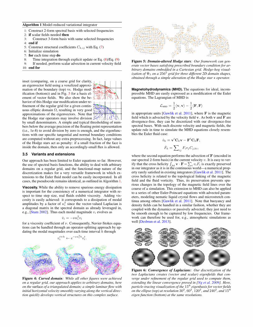
Algorithm 1 Model-reduced variational integrator

1: Construct 2-form spectral basis with selected frequencies2: if scalar fields needed then3: Construct 3-form basis with same selected frequencies4: end if5: Construct structural coefficients Ck,ij with Eq. (7)6: Initialize simulation7: for each time step do8: Time integration through explicit update or Eq. (8)/Eq. (9)9: If needed, perform scalar advection in current velocity field

10: end for

inset (comparing, on a coarse grid for clarity,an eigenvector field using a voxelized approxi-mation of the boundary (top) vs. Hodge mod-ification (bottom)) and in Fig. 5 for a basis el-ement of vector fields. We also show the be-havior of this Hodge star modification under re-finement of the regular grid for a given contin-uous elliptic domain Ω, resulting in very goodapproximations of the eigenvectors. Note thatthe Hodge star operators may involve divisionby small denominators. A simple and typical thresholding of num-bers below the average precision of the floating point representation(i.e., 1e-8) to avoid division by zero is enough, and the eigenfunc-tions with our specific tangential and normal boundary conditionsare computed without any extra preprocessing. In fact, large valuesof the Hodge stars act as penalty: if a small fraction of the face isinside the domain, then only an accordingly-small flux is allowed.

3.5 Variants and extensions

Our approach has been limited to Euler equations so far. However,the use of spectral basis functions, the ability to deal with arbitrarydomains on a regular grid, and the functional-map nature of thediscretization makes for a very versatile framework in which ex-tensions to the Euler fluid model can be easily incorporated. In allcases, the pseudocode remains identical, as outlined in Algorithm 1.

Viscosity. While the ability to remove spurious energy dissipationis important for the consistency of a numerical integrator with re-spect to time step size, real fluids exhibit viscosity. Adding vis-cosity is easily achieved: it corresponds to a dissipation of modalamplitudes by a factor of κ2

i since the vector-valued Laplacian isa diagonal matrix in the spectral domain as already leveraged in,e.g., [Stam 2002]. Thus each modal magnitude vi evolves as

vi = −νκ2i vi

for a viscosity coefficient of ν. Consequently, Navier-Stokes equa-tions can be handled through an operator-splitting approach by up-dating the modal magnitudes over each time interval h through

vt+hi ← e−νκ2ihvti .

Figure 4: Curved domain: While all other figures were achievedon a regular grid, our approach applies to arbitrary domains, hereon the surface of a triangulated domain; a simple laminar flow withinitial horizontal velocity smoothly varying along the vertical direc-tion quickly develops vortical structures on this complex surface.

Figure 5: Domain-altered Hodge stars: Our framework can gen-erate vector bases satisfying prescribed boundary condition for ar-bitrary domains embedded in a Cartesian grid. Hedge-hog visual-ization of Ψ5 on a 2562 grid for three different 2D domain shapes,obtained through a simple alteration of the Hodge star ? operator.

Magnetohydrodynamics (MHD). The equations for ideal, incom-pressible MHD are easily expressed as a modification of the Eulerequations. The Lagrangian of MHD is

LMHD =1

2〈v,v〉 − 1

2〈F,F〉

in appropriate units [Gawlik et al. 2011], where F is the magneticfield which is advected by the velocity field v. As both v and F aredivergence-free, they can be discretized with our divergence-freespectral bases. With such discrete velocity and magnetic fields, theupdate rule in time to simulate the MHD equations closely resem-bles the Euler fluid case:

vk = vtCkv − FtCkF,

Fk =∑

ijFivjCj,ki,

where the second equation performs the advection of F (encoded inour spectral 2-form basis) in the current velocity v. It is easy to ver-ify that the cross helicity

∫M v · F=

∑i viFi is exactly preserved

in our integrator as it is in the continuous world—a numerical prop-erty rarely satisfied in existing integrators [Gawlik et al. 2011]. Thecross helicity is related to the topological linking of the magneticfield and the fluid vorticity. Thus, its preservation prevents spu-rious changes in the topology of the magnetic field lines over thecourse of a simulation. This extension to MHD can also be appliedto a series of other Euler-Poincare equations with advected param-eters, modeling nematic liquid crystal flows and microstretch con-tinua among others [Gawlik et al. 2011]. Note that buoyancy anddensity fields can be handled in a similar fashion, whether they arecoupled with the dynamics or passively advected; they just need tobe smooth enough to be captured by low frequencies. Our frame-work can therefore be used for, e.g., atmospheric simulations aswell [Desbrun et al. 2013].

Figure 6: Convergence of Laplacians: Our discretization of thetwo Laplacians creates (vector and scalar) eigenfields that con-verge under refinement of the regular grid used to compute them,extending the linear convergence proved in [Ng et al. 2009]. Here,particle-tracing visualization of the 15th eigenbasis for vector fieldson the ellipse (top) at resolution 302, 602, 1202, and 2402, and 15th

eigen function (bottom) at the same resolutions.

Subgrid scale modeling. Direct numerical solvers using NavierStokes equation require high resolutions to resolve the correct cou-pling of large and small scale structures. Instead, subgrid scalemodeling requires much fewer degrees of freedom to capture thecorrect large-scale structures by simulating the main effects ofthe small subgrid scale structures without actually resolving them.Among the many models that match empirical data well, the LANS-α model (Lagrangian-Averaged-Navier-Stokes, see [Foias et al.2002]) advects the velocity in a filtered velocity to better capturethe correct energy cascading. Since filtering is achieved through aLaplacian-based Helmholtz operator, we can also use our spectralapproach to simulate this model with ease. The kinetic energy (i.e.,Lagrangian) is now defined as

Lα-Euler =

∫M

1

2v2 +

α2

2|∇v|2.

In our spectral bases, the α-model amounts to adding kinetic energyterms scaled by κ2

i for the modal amplitudes vi. Hamilton’s princi-ple for the modified Lagrangian leads to essentially the same updaterule as Navier-Stokes’, except that the structural coefficients are re-placed by (1 + α2κ2

i )Ck,ij . Note that this modification keeps theantisymmetry in j and k intact, and is therefore a trivial alterationof the basic scheme.

Figure 7: Spectral energy distribution: With forcing terms keep-ing the low wave number amplitudes fixed [Foias et al. 2002], our3D reduced model applied to the LANS-α model of turbulence pro-duces an average spectral energy distribution (blue) much closerto the expected Kolmogorov distribution (black) than with the usualNavier-Stokes equations (red).

Moving obstacles and external forces. For moving obstacles, in-stead of calculating additional boundary bases as in [Treuille et al.2006], we instead follow the simpler solution proposed in [De Wittet al. 2012]: the difference in the normal component of the velocityon the boundary is projected onto the velocity basis and subtractedfrom v, resulting in a low-frequency field roughly satisfying theboundary condition. For any external forces, e.g., buoyancy forces,their effects on the time derivative of the modal amplitude vi of thei-th frequency are simply calculated by their projection onto Ψi.The results are visually correct even on complex shapes, and withminimal computational overhead (see Fig. 10).

3.6 Generalization to other bases

While we provided detail on the construction of a variationalmodel-reduced integrator for fluid simulation using Laplace eigen-vectors, one can easily adapt our approach to arbitrary basis func-tions, even those extracted from a training set of fluid motions.Suppose that we are given a set of scalar basis elements Φi (or-thonormalized through the Gram-Schmidt procedure) and a set ofvelocity basis elements Ψi. The Lie derivative matrixAwill still beantisymmetric as long as Ψi’s are divergence-free. This means thatone can use existing finite element basis functions instead of ourLaplace eigenvectors—or even wavelet bases of H(div,Ω) (see,e.g., [Urban 2002]) if spatially localized basis functions are sought

Figure 8: Smoke rising. Using only 230 modes (about 0.003% ofthe full spectrum simulation), both [De Witt et al. 2012]’s (left) andour approach already exhibit the expected volutes for a buoyancy-driven flow over a sphere.

after to get a sparser advection. The key to the numerical benefits ofour variational approach is to ensure the anti-commutativity of theLie bracket in the evaluation of 〈Ai, [Aj , Ak]〉 (Eq. (7)) and the ad-vection of other fields by the exponential map (or approximationsthereof, see App. D) of the matrix representing the Lie derivativeas done in MHD and complex fluids [Gawlik et al. 2011]. In away, the original non-spectral variational integrators can be seen asa special case of our framework where Whitney basis functions areused. However, viscosity can no longer be handled as easily in thiscase as the Laplacian is not diagonal in general bases. Moreover,the required number of degrees of freedom to produce smooth flowsmay end up being high if the bases are arbitrary.

4 ResultsOur results were generated on an Intel i7 laptop with 12GB RAM,and visualized using our own particle-tracing and rendering tools.

Reduced vs. full simulation. In order to check the validity of ourreduced approach, we performed a stress test in a periodic 2D do-main to visualize how the increase in the number of bases used inour spectral integrator impacts the simulation over time. We se-lected a band-limited initial velocity field at time t = 0 that onlycontains non-zero components for the first 120 frequencies. Wethen advected the fluid using our integrator, with fluid markersinitially set as two colored disks near the center. Because of thepropensity of vorticity to go to higher scales, our reduced approachdoes not lead to the exact same position of the fluid markers af-ter 12s of simulation if one uses only 120 bases. However, as thenumber of bases increases to 300 or 500, the simulation quicklycaptures the same dynamical behavior as a full variational integra-tor with 2562 degrees of freedom, see Fig. 9. We demonstrate inthe accompanying video that our variational integrator also capturesthe proper qualitative behavior of two merging vortices in contrastto the result using [De Witt et al. 2012] which, instead, generatesseveral vortices (see supplementary video).

Figure 9: Convergence of simulation: A flow in a periodic do-main is initialized with a band-limited velocity fields with 120 wavenumber vectors. Fluid markers (forming a blue and red circle) areadded for visualization. After 12s of simulation, the results of ourreduced approach (left: 120, middle: 300 modes) vs. the full 2562

dynamics (right) are qualitatively similar.

Figure 10: Interactivity: We can also use the analytic expressionsfor Ψk andCk,ij in a periodic 3D domain to handle a large numberof modes directly. The explicit update rule exhibits no artificialdamping of the energy as expected, but offers realtime flows.

Arbitrary domains. We also show in Figs. 3, 5, and 11 (2D) andFigs. 1, 2, 8, 14, and 10 (3D) that the use of boundary condi-tions embedded on regular grids leads to the expected visual be-havior near domain boundaries, eliminating the staircase artifactsof traditional immersed-grid methods. Our homogenized boundarytreatment obtains results similarto those of unstructured mesheswhile using only calculations thatare directly performed on regulargrids—thus requiring significantlysimpler, smaller, and more effi-cient data structures. As shown inthe log(error)-log(resolution) plotin the inset, our basis fields con-verge with second order accuracy,much faster than the boundary condition in [Batty et al. 2007] (thelatter may, in fact, not even converge in some cases as discussedin [Ng et al. 2009]). Moreover, we also extended this approach notjust to scalar field, but vector fields. Our fluid dynamics is also con-sistent across a wide range of temporal and spatial discretizations,see Fig. 11. In addition, the regular grid structure also simplifies theinteraction with immersed solid objects as demonstrated in Fig. 14through a flow induced by a scripted car turning around a corner;interactive fluid stirring by a paddle manipulated by the user is alsoeasily achieved as shown in Fig. 10. We also show in Fig. 8 thatour method can handle the typical test case of smoke plume past asphere even at low resolution, and we can incorporate both free-slipor no-slip boundary conditions. Finally, our spectral integrator canbe carried out in the same fashion on curved domains as well, sincethe eigenvectors of the Laplace(-Beltrami) operator are no more dif-ficult to compute on a triangulated surface; Fig. 4 shows a simplelaminar flow on the surface of the bunny model.

Advanced fluid models. We also extended our method to theLANS-α turbulence model to better capture the spectral energy dis-tribution with a small number of modes. On a 3D regular grid, weperformed a simulation as described in [Foias et al. 2002] by hold-ing the low wave number components vi fixed for |κi| < 2 to actas a forcing term, and running the simulation until t = 100. Wethen extracted the average spectral energy distribution present be-tween t= 33 to t= 100. We show in Fig. 7 that the Kolmogorov“−5/3 law” is much better captured than with the usual Navier-Stokes model, even for the low number of modes used in our spec-tral context: the α-model produces a decay rate at high wave num-bers much steeper than a Navier-Stokes simulation, allowing us tocut off the higher frequencies at a lower threshold without signifi-cant deviation from the spectral distribution. This indicates that ourapproach consisting in a simple scaling of the structural coefficientshelps improving fluid simulation on coarse grids.

We also implemented our extension to MHD, and found the ex-pected preservation of cross-helicity and energy. For comparisonpurposes (see, e.g., [Gawlik et al. 2011]), we visualize our resultsof the typical rotor test with 100 modes in Fig. 15. We finally showin Figs. 2 and 8 that buoyancy forces are also easy to incorporateby adding an upwards force proportional to the local smoke tem-

Figure 11: Robustness to resolution: With the homogenizedboundary condition on grids of resolution 402 (blue), 802 (green),and 1602 (red), no staircase artifacts are observed, and the simu-lation results are consistent across resolutions.

perature; the curl of this external force is projected onto the 1-formbasis functions, and used to update the vorticity.

Computational efficiency. Our use of model reduction via Lapla-cian eigenbases provides a significantly more efficient alternative tofull simulators, obviously. Due to our variational treatment of timeintegration, we also prevent many shortcomings of the previous re-duced models as we ensure consistency of the results over a largespectrum of spatial and temporal discretization rates, and maintain aqualitatively correct behavior even on coarse grids. The efficiencygain compared to the full variational simulation is apparent, be itin 2D, curved 2D, or 3D. For instance, a full-blown 1282 grid takesaround 50s for the variational integrator to update one step (througha Newton solver) in a typical simulation using the trapezoidal ruleupdate, while a 50-mode (resp., 100-mode and 200-mode) simula-tion with our integrator takes only 0.098s (resp., 0.65s and 2.0s) forcomplex boundaries (i.e., with dense structural coefficients), and0.026s (resp., 0.070s, 0.28s) for simple box domains (with sparsecoefficients). Our Newton solver normally converges in a coupleof iterations depending on the time step size (which determines thequality of the initial guess); for instance, the average in our 3Dbunny buoyancy test in Fig. 2 is below 3 iterations.

Selection of frequencies. Depending on how many modes theuser is willing to discard (and replace by wavelet noise or dynam-ical texture for efficiency), the computational gains can be in theorder of several orders of magnitude, and this allows us to simu-late flows at interactive or realtime rates (see Fig. 14, or Fig. 10 foran example with a periodic 3D domain where we can compute theeigenbases in closed form). Note however that our model-reducedintegrator suffers from the usual limitation of model reduction: thecomplexity is actually growing quadratically (resp., cubically) withthe number of modes for sparse (resp., dense) structural coeffi-cients. So our integrator is numerically efficient only for relativelylow mode counts. However, this is exactly the regime for whichone can achieve significant computational savings for very little vi-sual degradation. Similar to [De Witt et al. 2012], we also foundthat, when using very few low frequencies leads to unappealingsimulations, adding a few high frequencies (and thus, skipping alarge amount of medium frequencies) is enough to render an ani-mation realistic: our integrator can use such a tailored frequencyrange seamlessly, and the non-linear exchange between low andhigh frequencies is enough to create much more complex patternsthat respect the expected motion of the flow, see Fig. 12. Fig 8 wasalso done in this manner: the first 115 modes were used, the next400 modes were skipped, and we added the next 115 modes to addsmall scale effects. The use of subgrid scale modeling explained in§3.5 is yet another way to make sure that the higher frequencies areproperly dealt with and provide a good, visually correct approxima-tion to the fluid equations.

Time stepping. Finally, an important feature of our model-reducedapproach is its ability to handle both explicit and implicit integra-tion. Implicit integration, using the midpoint rule (Eq. (8)) or the

trapezoidal rule (Eq. (9)), come with good numerical guaranteesdue to the time reversibility. However, explicit integration is alsovery convenient as it further reduces the time complexity of thesimulation. Nevertheless, an explicit integration has very little the-oretical guarantees, and should only be used with care.

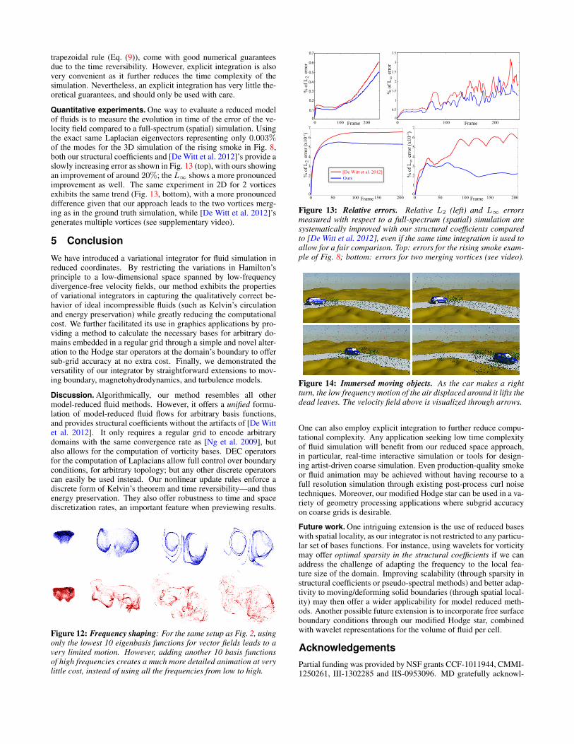
Quantitative experiments. One way to evaluate a reduced modelof fluids is to measure the evolution in time of the error of the ve-locity field compared to a full-spectrum (spatial) simulation. Usingthe exact same Laplacian eigenvectors representing only 0.003%of the modes for the 3D simulation of the rising smoke in Fig. 8,both our structural coefficients and [De Witt et al. 2012]’s provide aslowly increasing error as shown in Fig. 13 (top), with ours showingan improvement of around 20%; the L∞ shows a more pronouncedimprovement as well. The same experiment in 2D for 2 vorticesexhibits the same trend (Fig. 13, bottom), with a more pronounceddifference given that our approach leads to the two vortices merg-ing as in the ground truth simulation, while [De Witt et al. 2012]’sgenerates multiple vortices (see supplementary video).

5 Conclusion

We have introduced a variational integrator for fluid simulation inreduced coordinates. By restricting the variations in Hamilton’sprinciple to a low-dimensional space spanned by low-frequencydivergence-free velocity fields, our method exhibits the propertiesof variational integrators in capturing the qualitatively correct be-havior of ideal incompressible fluids (such as Kelvin’s circulationand energy preservation) while greatly reducing the computationalcost. We further facilitated its use in graphics applications by pro-viding a method to calculate the necessary bases for arbitrary do-mains embedded in a regular grid through a simple and novel alter-ation to the Hodge star operators at the domain’s boundary to offersub-grid accuracy at no extra cost. Finally, we demonstrated theversatility of our integrator by straightforward extensions to mov-ing boundary, magnetohydrodynamics, and turbulence models.

Discussion. Algorithmically, our method resembles all othermodel-reduced fluid methods. However, it offers a unified formu-lation of model-reduced fluid flows for arbitrary basis functions,and provides structural coefficients without the artifacts of [De Wittet al. 2012]. It only requires a regular grid to encode arbitrarydomains with the same convergence rate as [Ng et al. 2009], butalso allows for the computation of vorticity bases. DEC operatorsfor the computation of Laplacians allow full control over boundaryconditions, for arbitrary topology; but any other discrete operatorscan easily be used instead. Our nonlinear update rules enforce adiscrete form of Kelvin’s theorem and time reversibility—and thusenergy preservation. They also offer robustness to time and spacediscretization rates, an important feature when previewing results.

Figure 12: Frequency shaping: For the same setup as Fig. 2, usingonly the lowest 10 eigenbasis functions for vector fields leads to avery limited motion. However, adding another 10 basis functionsof high frequencies creates a much more detailed animation at verylittle cost, instead of using all the frequencies from low to high.

Figure 13: Relative errors. Relative L2 (left) and L∞ errorsmeasured with respect to a full-spectrum (spatial) simulation aresystematically improved with our structural coefficients comparedto [De Witt et al. 2012], even if the same time integration is used toallow for a fair comparison. Top: errors for the rising smoke exam-ple of Fig. 8; bottom: errors for two merging vortices (see video).

Figure 14: Immersed moving objects. As the car makes a rightturn, the low frequency motion of the air displaced around it lifts thedead leaves. The velocity field above is visualized through arrows.

One can also employ explicit integration to further reduce compu-tational complexity. Any application seeking low time complexityof fluid simulation will benefit from our reduced space approach,in particular, real-time interactive simulation or tools for design-ing artist-driven coarse simulation. Even production-quality smokeor fluid animation may be achieved without having recourse to afull resolution simulation through existing post-process curl noisetechniques. Moreover, our modified Hodge star can be used in a va-riety of geometry processing applications where subgrid accuracyon coarse grids is desirable.

Future work. One intriguing extension is the use of reduced baseswith spatial locality, as our integrator is not restricted to any particu-lar set of bases functions. For instance, using wavelets for vorticitymay offer optimal sparsity in the structural coefficients if we canaddress the challenge of adapting the frequency to the local fea-ture size of the domain. Improving scalability (through sparsity instructural coefficients or pseudo-spectral methods) and better adap-tivity to moving/deforming solid boundaries (through spatial local-ity) may then offer a wider applicability for model reduced meth-ods. Another possible future extension is to incorporate free surfaceboundary conditions through our modified Hodge star, combinedwith wavelet representations for the volume of fluid per cell.

AcknowledgementsPartial funding was provided by NSF grants CCF-1011944, CMMI-1250261, III-1302285 and IIS-0953096. MD gratefully acknowl-

edges all the members of the TITANE team and the Inria Interna-tional Chair program for support.

ReferencesAN, S., KIM, T., AND JAMES, D. 2008. Optimizing cubature

for efficient integration of subspace deformations. ACM Trans.Graph. 27, 5, Art. 165.

ARNOLD, D. N., FALK, R. S., AND WINTHER, R. 2006. Finiteelement exterior calculus, homological techniques, and applica-tions. Acta Numerica 15, 1–155.

AZENCOT, O., WEISSMANN, S., OVSJANIKOV, M., WARDET-ZKY, M., AND BEN-CHEN, M. 2014. Functional fluids onsurfaces. Comput. Graph. Forum 33, 5, 237–246.

BATTY, C., BERTAILS, F., AND BRIDSON, R. 2007. A fast varia-tional framework for accurate solid-fluid coupling. ACM Trans.Graph. 26, 3, Art. 100.

BELL, N., AND HIRANI, A. N., 2008. PyDEC: A Python li-brary for Discrete Exterior Calculus. Google Code project at:http://code.google.com/p/pydec/.

CHORIN, A., AND MARSDEN, J. 1979. A Mathematical Introduc-tion to Fluid Mechanics, 3rd edition ed. Springer-Verlag.

COHEN, J. M., TARIQ, S., AND GREEN, S. 2010. Interac-tive fluid-particle simulation using translating Eulerian grids. InACM Symp. on Interactive 3D Graphics and Games, 15–22.

DE WITT, T., LESSIG, C., AND FIUME, E. 2012. Fluid simulationusing Laplacian eigenfunctions. ACM Trans. Graph. 31, 1, Art.10.

DESBRUN, M., KANSO, E., AND TONG, Y. 2008. Discrete differ-ential forms for computational modeling. In Discrete Differen-tial Geometry, A. I. Bobenko et al., Ed., vol. 38 of OberwolfachSeminars. Birkhauser Basel, 287–324.

DESBRUN, M., GAWLIK, E. S., GAY-BALMAZ, F., ANDZEITLIN, V. 2013. Variational discretization for rotating strati-fied fluids. Disc. Cont. Dyn. S. 34, 2, 477–509.

ELCOTT, S., AND SCHRODER, P. 2006. Building your own DECat home. In Discrete Differential Geometry, ACM SIGGRAPHCourses, 55–59.

ELCOTT, S., TONG, Y., KANSO, E., SCHRODER, P., AND DES-BRUN, M. 2007. Stable, circulation-preserving, simplicial flu-ids. ACM Trans. Graph. 26, 1, Art. 4.

FELDMAN, B. E., O’BRIEN, J. F., AND KLINGNER, B. M. 2005.Animating gases with hybrid meshes. ACM Trans. Graph. 24, 3,904–909.

FOIAS, C., HOLM, D. D., AND TITI, E. S. 2002. The three di-mensional viscous Camassa–Holm equations, and their relationto the Navier–Stokes equations and turbulence theory. J. Dyn.Differ. Equ. 14, 1, 1–35.

FOSTER, N., AND METAXAS, D. 1997. Modeling the motion of ahot, turbulent gas. In Proc. ACM SIGGRAPH, 181–188.

GAO, Y., LI, C.-F., REN, B., AND HU, S.-M. 2013. View-dependent multiscale fluid simulation. IEEE Trans. Vis. Comput.Graph. 19, 2, 178–188.

GAWLIK, E., MULLEN, P., PAVLOV, D., MARSDEN, J., ANDDESBRUN, M. 2011. Geometric, variational discretization ofcontinuum theories. Physica D: Nonlinear Phenomena 240, 21,1724–1760.

GOLAS, A., NARAIN, R., SEWALL, J., KRAJCEVSKI, P., DUBEY,P., AND LIN, M. 2012. Large-scale fluid simulation usingvelocity-vorticity domain decomposition. ACM Trans. Graph.31, 6, Art. 148.

GUPTA, M., AND NARASIMHAN, S. G. 2007. Legendre fluids: Aunified framework for analytic reduced space modeling and ren-dering of participating media. In Symp. on Computer Animation,17–25.

HARLOW, F. H., AND WELCH, J. E. 1965. Numerical calculationof time-dependent viscous incompressible flow of fluid with freesurface. Physics of Fluids 8, 12, 2182–2189.

HOWES, R., SCHROEDER, C., AND TERAN, J. M. 2013. A vir-tual node algorithm for Hodge decompositions of inviscid flowproblems with irregular domains. Methods Appl. Anal. 20, 4,439–455.

KHAREVYCH, L., YANG, W., TONG, Y., KANSO, E., MARSDEN,J. E., SCHRODER, P., AND DESBRUN, M. 2006. Geomet-ric, variational integrators for computer animation. In Symp. onComputer Animation, 43–51.

KIM, T., AND DELANEY, J. 2013. Subspace fluid re-simulation.ACM Trans. Graph. 32, 4, 62.

KIM, T., THUREY, N., JAMES, D., AND GROSS, M. 2008.Wavelet turbulence for fluid simulation. In ACM Trans. Graph.,vol. 27, ACM, 50.

LI, S., HUANG, J., DE GOES, F., JIN, X., BAO, H., AND DES-BRUN, M. 2014. Space-time editing of elastic motion throughmaterial optimization and reduction. ACM Trans. Graph. 33, 4,Art. 108.

LONG, B., AND REINHARD, E. 2009. Real-time fluid simulationusing discrete sine/cosine transforms. In Symp. on Interactive3D Graphics and Games, 99–106.

LOSASSO, F., TALTON, J., KWATRA, N., AND FEDKIW, R. 2008.Two-way coupled SPH and Particle Level Set fluid simulation.IEEE Trans. Vis. Comput. Graph. 14, 4, 797–804.

MARSDEN, J. E., AND WEST, M. 2001. Discrete mechanics andvariational integrators. Acta Numerica 2001 10, 357–514.

MULLEN, P., CRANE, K., PAVLOV, D., TONG, Y., AND DES-BRUN, M. 2009. Energy-preserving integrators for fluid anima-tion. ACM Trans. Graph. 28, 3, Art. 38.

NARAIN, R., SEWALL, J., CARLSON, M., AND LIN, M. C. 2008.Fast animation of turbulence using energy transport and proce-dural synthesis. ACM Trans. Graph. 27, 5, 166.

NG, Y. T., MIN, C., AND GIBOU, F. 2009. An efficient fluid-solidcoupling algorithm for single-phase flows. J. Comput. Phys. 228,23, 8807–8829.

ORSZAG, S. A. 1969. Numerical methods for the simulation ofturbulence. Physics of Fluids 12, II 250–257.

PAVLOV, D., MULLEN, P., TONG, Y., KANSO, E., MARSDEN, J.,AND DESBRUN, M. 2011. Structure-preserving discretizationof incompressible fluids. Physica D: Nonlinear Phenomena 240,6, 443–458.

SCHECHTER, H., AND BRIDSON, R. 2008. Evolving sub-grid tur-bulence for smoke animation. In Symp. on Computer Animation,1–7.

SELLE, A., RASMUSSEN, N., AND FEDKIW, R. 2005. A vortexparticle method for smoke, water and explosions. ACM Trans.Graph. 24, 3, 910–914.

SILBERMAN, I. 1954. Planetary waves in the atmosphere. J. Me-teor. 11, 27–34.

STAM, J., AND FIUME, E. 1993. Turbulent wind fields for gaseousphenomena. In Proc. ACM SIGGRAPH, 369–376.

STAM, J. 1999. Stable fluids. In Proc. ACM SIGGRAPH, 121–128.

STAM, J. 2002. A simple fluid solver based on the FFT. J. Graph.Tools 6, 2, 43–52.

STAM, J. 2003. Flows on surfaces of arbitrary topology. ACMTrans. Graph. 22, 3, 724–731.

STANTON, M., SHENG, Y., WICKE, M., PERAZZI, F., YUEN, A.,NARASIMHAN, S., AND TREUILLE, A. 2013. Non-polynomialGalerkin projection on deforming meshes. ACM Trans. Graph.32, 4, Art. 86.

STEINHOFF, J., AND UNDERHILL, D. 1994. Modification of theEuler equations for Vorticity Confinement. Physics of Fluids 6,8, 2738–2744.

TONG, Y., ALLIEZ, P., COHEN-STEINER, D., AND DESBRUN,M. 2006. Designing quadrangulations with discrete harmonicforms. In Symp. on Geometry Processing, 201–210.

TREUILLE, A., LEWIS, A., AND POPOVIC, Z. 2006. Model re-duction for real-time fluids. ACM Trans. Graph. 25, 3, 826–834.

URBAN, K. 2002. Wavelet bases for H(div) and H(curl). InWavelets in Numerical Simulation, vol. 22 of Lecture Notes inComputational Science and Engineering. 83–107.

VON TYCOWICZ, C., SCHULZ, C., SEIDEL, H.-P., AND HILDE-BRANDT, K. 2013. An efficient construction of reduced de-formable objects. ACM Trans. Graph. 32, 6, Art. 213.

YUAN, Z., CHEN, F., AND ZHAO, Y. 2011. Pattern-guided smokeanimation with Lagrangian Coherent Structure. ACM Trans.Graph. 30, 6, Art. 136.

YUDOVICH, V. 1963. Non-stationary flow of an ideal incompress-ible liquid. USSR Computational Mathematics and Mathemati-cal Physics 3, 6, 1407–1456.

ZHANG, X., BRIDSON, R., AND GREIF, C. 2015. Restoringthe missing vorticity in advection-projection fluid solvers. ACMTrans. Graph. 34, 4, Art. 52.

A Computing spectral basesIn this appendix, we describe how to compute the spectral bases forboth vector fields and density fields on a meshM.

Discrete Laplacians. Finding our spectral bases first requires dis-cretizing both the scalar Laplacian ∇·∇ and the vector Laplacian−∇×∇×+∇∇· on the domainM. Discretization of these opera-tors on arbitrary simplicial complexes is well documented [Desbrunet al. 2008; Elcott and Schroder 2006], and only involves topolog-ical operators d1 and d2 deriving from the mesh connectivity, anddiagonal “Hodge star” operators ?1, ?2, and ?3 based on local mea-sures of M and its circumcentric dual, resulting in the followingsymmetric second-order operators:

?3∆3 ≡ ?3d2 ?−12 dt2?3, ?2∆2 ≡ dt2 ?3 d2+?2d1 ?

−11 dt1 ?2 .

Note that d and ? are even simpler on regular grids, even with thealteration we introduced in 3.4.

Figure 15: MHD rotor test: The rotor test for magnetohy-drodynamics consists of a dense rotating disk of fluid in aninitially uniform magnetic field (left-right, top-middle: t =0.042, 0.126, 0.210, 0.336). Our spectral integrator captures thecorrect behavior (see full dynamics in [Gawlik et al. 2011]) evenwith only 100 modes. Discrete energy (blue) and cross-helicity(red) are, as predicted, preserved over time (bottom).

Boundary conditions. The canonical boundary conditions of ve-locity fields in fluid simulation for graphics purposes are no-transfer(i.e., the normal component vn of the velocity along ∂M must bezero) and free-slip (i.e., the derivative of the tangential velocity fieldalong the boundary normal ∂vt/∂n must be zero as well). To en-force these conditions, we thus add the conditions that the flux ofΨi on every boundary face is zero, and that the circulations alongthe (interior half) boundary of the Voronoi face associated with eachboundary edge is also zero (i.e, we simply set the values of ?−1

1 aszeros for all the edges adjacent to the boundary faces to compute∆2). As for the eigenfunctions Φi of ∆3, we use either Dirich-let boundary conditions f |∂M = 0 or Neumann boundary condi-tions ∂f

∂n|∂M = 0, by considering boundary cell values or boundary

gradients as null. If other, non-homogeneous boundary conditions(such as influx or outflux conditions) are required, then one mustadd an additional harmonic (zeroth frequency) component that sat-isfies the given boundary conditions.

Eigen computations. Once the Laplacians with proper boundaryconditions are assembled, we can compute their low-frequencyeigenfields using a simple Lanczos algorithm since these operatorsare symmetric. The constant eigenbases from the kernel of ∆3 canbe safely omitted by setting zero values on boundaries, since a con-stant scalar function is unchanged when advected by a divergence-free velocity field. Note that, as mentioned in §3.1, some of theeigenfields Ψi will be of the form 1/µjδΦj : indeed, δΦi for i 6= 0is an eigenfunction of ∆2 since

∆2δΦj = δ∆3Φj = δ(−µ2jΦj) = −µ2

jδΦj .

These gradient fields are easily identifiable by checking their di-vergence. Note finally that in theory, there could be cases whereκ2i =µ2

j for multiple pairs of indices i and j. While in practice thisis very unlikely to happen, one can protect against this rare event byreplacing one of the corresponding Ψi by δΦj/µj , and replacingthe other eigenvectors of this eigenvalue through a Gram-Schmidtprocess to form an orthonormal basis again.

Comments. We note that the approach we described above to com-pute the eigen bases for our fluid integrator is far from unique. Forexample, the β1 harmonic vector fields are obtained as the eigen-vectors associated with the eigenvalue 0, but we could have alsocomputed the harmonic function dual to each homology generatorvia simple sparse linear systems instead [Tong et al. 2006]. Ad-ditionally, the vector field basis Ψi could be computed through itsvector potential ψi instead: indeed, these vector potential 1-formsare eigenvectors of the 1-form Laplacian ∆1, and boundary edgecirculations as well as divergence on boundary dual cell divergenceare assumed null to guarantee no-transfer and free-slip conditions.The curl of these 1-form basis functions are then, by construction,the flux-based Ψi basis functions. Finally, we point out that ourapproach is purposely different from what is proposed in [De Wittet al. 2012], as they use an eigendecomposition of dδ instead (lever-aging the divergence-freeness of the vector fields). However, thissimplified operator has a much larger null space that includes alsocurl-free fields, requiring many more eigenvectors to be computedvia Lanczos iterations to generate divergence-free fields.

B Analysis of structural coefficients Ck

For simplicity, we use the periodic domain [0, 1]3, i.e., the flat 3Dtorus. The eigenfields can be expressed using complex numbers as

Ψi(x) = wieki·x,

where is the unit imaginary number, x is the 3D coordinates, wi

is a unit vector, and ki is the wave number vector (i.e., with |ki| =κi). The divergence of the basis function is thus

divΨi(x) = ki ·wieki·x,

while the curl is expressed as

curlΨi(x) = ki ×wieki·x.

Since divΨi = 0 means that ki ·wi = 0, there are two independentw’s for each k in the basis. We can thus compute the structuralcoefficients Cc,ab from Eq. (7) in closed form, by the integral of

(∇×Ψa) · (Ψ∗c×Ψb) = (ka×wa) · (wc×wb)e(ka+kb−kc)·x,

where superscript ∗ denotes complex conjugation. Note thatnonzero coefficients (ka×wa)·(wc×wb) only exist when kc =ka+kb, and they advect real fields to real fields (whose coefficientssatisfy vk,w = v∗−k,w). It indicates that |kb|2Cc,ab = |ka|2Cc,bais not true in general in 3D, contrary to the claim in [De Witt et al.2012]; a simple counterexample is ka=2π(0, 2, 3), wa=(1, 0, 0),kb = 2π(1, 1, 0), and wb = (0, 0, 1). Moreover, while Cc,aa = 0indeed for this domain since wc · (2ka) = 0, this property willno longer hold for an arbitrary domain. Thankfully, our variationalintegrator does not depend on the eigenmodes being steady flows,so these symmetries (or rather, lack thereof) are inconsequential.

C Kelvin’s circulation theoremIdeal, incompressible fluids have a conserved momentum [Chorinand Marsden 1979] given by the integrated circulation of the fluidaround a closed curve which is advected by the flow. This fact isknown as Kelvin’s circulation theorem. Methods such as [Elcottet al. 2007] and [Pavlov et al. 2011] are constructed so as to con-serve a discretized form of this conserved momentum. Our spectralmethod also obeys a form of Kelvin’s theorem as follows. We candefine generalized “spectral” curves as spectral dual 1-chains (alsocalled 1-currents [Desbrun et al. 2008]) of the form:

Γ =∑i

γi ?2 Ai. (10)

The above dual 1-chain expression always represents a closedcurve, because each Ai corresponds to a closed (divergence-free)

2-form, which means the dual 1-chain is boundaryless. A pairingbetween a 2-form and a generalized loop is defined as expected:

〈A,Γ〉 =

⟨∑i

viAi,∑j

γj ?2 Aj

⟩=∑i

viγi. (11)

The Lie advection of the generalized curve along the velocity field

Γ = −[A,Γ] (12)

indicates that the coefficients γii must evolve such that

γk = −∑i,j

γivj

∫M

Ψk · (∇× (Ψi ×Ψj))

=∑i,j

γivj

∫M

(∇×Ψk) · (Ψj ×Ψi) =∑i,j

γivjCj,ki.

Thus, the spectral version of Kelvin’s theorem holds since

d

dt〈A,Γ〉 =

∑i

(viγi + viγi)

=∑i

vtCivγi+∑i

vi∑j,k

vkγjCk,ij

=∑i,j,k

vjCi,jkvkγi−∑i,j,k

vjvkγiCi,jk = 0.

In the above derivation, dummy index variables are swapped andthe identity Ck,ij = −Cj,ik is used.

D Temporal discretizationA fully discrete (in space and time) treatment of our variationalintegrator is easily achieved using the Hamilton-Pontryagin princi-ple [Kharevych et al. 2006], where Lagrange multipliers µk enforcethat A is indeed the Eulerian velocity of state q. If one denotes byh is the time step, Ak the velocity field between time k & stateqk and time k+1 & state qk+1, the discrete Hamilton-Pontryaginaction between t = 0 and t = Nh is expressed as

Sd =

N−1∑k=0

1

2〈Ak, Ak〉h+ 〈µk, τ−1(qk+1(qk)−1)− hAk〉.

The map τ must convert an element of the Lie algebra to a Liegroup element, thus making Ak the Eulerian velocity between timetk and tk+1; instead of the usual exponential map which is com-putationally difficult to handle, we approximate it to be the Cayleytransform τ(A)=(I−A/2)−1(I+A/2), as it efficiently maps anti-symmetric matrices to orthogonal matrices. Taking variations withrespect to µk, we recover the expected group element update rule

qk+1 = τ(hAk)qk.

Variations with respect to Ak show that the multiplier is actuallythe momentum: µk = Ak. Finally variations with respect to qk

restricted to δqk = Bkqk with Bk in the Lie algebra (to enforceLin constraints) yield

〈µk−1, (I − hAk−1/2)Bk(I + hAk−1/2)〉

= 〈µk, (I + hAk/2)Bk(I − hAk/2)〉.

Omitting the cubic terms inO(h2) still preserves a discrete Kelvin’stheorem, so we follow the suggestion in [Gawlik et al. 2011] andsimplify the update rule to

∀Bk, 〈Ak−1, Bk +h

2[Bk, Ak−1]〉 = 〈Ak, Bk +

h

2[Bk,−Ak]〉,

which reduces to the trapezoidal rule with Ak =∑i vki Ai and an

arbitrary Bk=∑i bkiAi.