model reduction of flow systems and networks by the ... · robert k. niven unsw canberra, act,...

Model Reduction of Flow Systems and

Networks by the Maximum Entropy Method

Model Reduction Across Disciplines, University of Leicester, UK, 20 August 2014

Robert K. Niven

UNSW Canberra, ACT, AustraliaInstitut PPrime, Poitiers, France

⎧⎨⎩

[email protected]

Bernd R. Noack Institut PPrime, Poitiers, France.

Marcus Abel Ambrosys GmbH / Univ. of Potsdam, Germany

Michael Schlegel T.U. Berlin, Germany

Steven H. Waldrip UNSW Canberra, ACT, Australia

Eurika Kaiser Institut PPrime, Poitiers, France

Funding from ARC, Go8/DAAD, CNRS, Region Poitou-Charentes

© R.K. Niven 4

Contents 1. MaxEnt analysis - justification + mathematical structure

2. MaxEnt in fluid mechanics - infinitesimal fluid element

3. MaxEnt in dynamical systems - oscillatory cylinder wake

4. MaxEnt analyses of flow networks - “standard” problem: flow rates + potentials - e.g. pipe flow system (nonlinear) - real example - “extended” problem: other uncertainties - chemical reaction networks

5. Conclusions

© R.K. Niven 5

Systems Analysis

© R.K. Niven 6

Probabilistic Systems Consider any system of discrete entities:

MaxEnt method (Jaynes, 1957, 1963, 2003)

- maximise entropy, subject to constraints → “least informative” description of system

MaxProb principle (Boltzmann, 1877; Planck, 1901) - maximise probability (⇒ entropy), subject to constraints → most probable state of system

e.g. atoms / molecules / ions, oscillators, quantum particles, fluid elements, motor vehicles, organisms, economic agents, social actors, humans, entire systems

© R.K. Niven 7

Boltzmann Principle (“MaxProb”)

H = lnP

N

P=N! qi

ni

ni !i=1

s∏

N→∞, ni /N→pi⎯ →⎯⎯⎯⎯⎯⎯⎯

H = − pi ln

piqii=1

s∑

Also pi→p(x)dx qi→q(x)dx

⎯ →⎯⎯⎯⎯⎯⎯⎯

H = − dx

−∞

∞

∫ p(x)ln p(x)q(x)

≡ Large Deviations theory (Ellis 1985) ≡ Method of Types (Csiszár, 1998)

{n.b. if P ≠ multinomial → different entropy function}

© R.K. Niven 8

Boltzmann Principle / MaxEnt / 2nd Law (Boltzmann, 1877; Planck, 1901 ↔ Jaynes 1957)

Weak Form “A system can be represented by its most probable state” → probabilistic inference - does not require asymptotic limit - does not give certainty Strong Form “A system tends towards its most probable state” - not just thermodynamics!

Inference

Ergodicity

© R.K. Niven 9

Contention: - identify MaxEnt / MaxProb solution with stationary state ⇒ dramatic simplification (model reduction) - old / new thermodynamics - fluid flow + non-equilibrium systems - other systems

Caveats: - probabilistic, not deterministic (this is inference !) - only infers the stationary state - discards the (unnecessary) dynamics

© R.K. Niven 10

Jaynes’ Mathematical Structure

© R.K. Niven 11

Jaynes’ MaxEnt Define probability pi over uncertainties i →

Maximise H = − pi ln

piqii=1

s∑ relative entropy

subject to

pii=1s∑ = 1 normalisation constraint

pii=1s∑ fri = ⟨fr ⟩, r = 1,...,R moment constraints

Write Lagrangian, extremise →

pi

* =qiZ

e− λr frir=1R∑ Boltzmann distribution

H* = lnZ + λr ⟨fr ⟩

r =1

R∑ maximum relative entropy

where λr = Lagrangian multipliers; Z = partition function

© R.K. Niven 12

Thermodynamic System (2 competing constraints) e.g.

pijj∑i∑ = 1 normalisation

pijεij∑i∑ = U mean energy

pijVjj∑i∑ = V mean volume

MaxEnt →

pij

* =qijZ

e−λEεi −λVVj

H* = lnZ + λE U + λV V

Identify S = kH* , λE = 1/ kT , λV = P / kT →

pij

* =qijZ

e−(εi +PVj )/kT

with qij ∝ degeneracy

S = k lnZ + U

T+ P V

T

© R.K. Niven 13

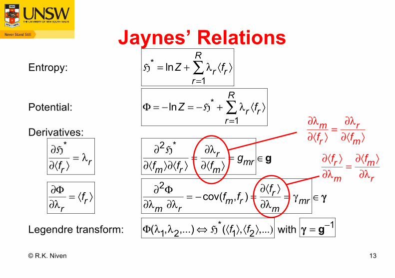
Jaynes’ Relations Entropy:

H* = lnZ + λr ⟨fr ⟩

r=1

R∑

Potential: Φ = − lnZ = −H* + λr ⟨fr ⟩

r=1

R∑

Derivatives:

∂H*

∂⟨fr ⟩= λr

∂2H*

∂⟨fm ⟩∂⟨fr ⟩=

∂λr∂⟨fm ⟩

= gmr ∈g

∂Φ∂λr

= ⟨fr ⟩

∂2Φ∂λm ∂λr

= −cov(fm,fr ) =∂⟨fr ⟩∂λm

= γmr ∈γγ

Legendre transform: Φ(λ1,λ2,...) ⇔ H*(⟨f1⟩,⟨f2⟩,...) with γ = g−1

∂⟨fr ⟩∂λm

=∂⟨fm ⟩∂λr

∂λm∂⟨fr ⟩

=∂λr∂⟨fm ⟩

© R.K. Niven 14

Thermodynamic System (c.f. Callen, 1985)

Entropy: S = k lnZ + U

T+ P V

T

Potential: kΦ = −k lnZ = −S + U

T+ P V

T= G

T Planck potential

i.e. G = kTΦ = −kT lnZ = −TS + U + P V Gibbs free energy

Derivatives:

∂S∂⟨U⟩

, ∂S∂⟨V ⟩

⎡⎣⎢

⎤⎦⎥= 1

T,PT

⎡⎣⎢

⎤⎦⎥

,

∂(G /T )∂(1/T )

,∂(G /T )∂(P /T )

⎡⎣⎢

⎤⎦⎥= ⟨U⟩,⟨V ⟩[ ]

Legendre transform:

GT

1T

,PT

⎛⎝⎜

⎞⎠⎟ ⇔ S(⟨U⟩,⟨V ⟩)

∂2(G /T )

∂(1/T )2∂2(G /T )

∂(1/T )∂(P /T )

∂2(G /T )∂(1/T )∂(P /T )

∂2(G /T )

∂(P /T )2

⎡

⎣

⎢⎢⎢⎢⎢

⎤

⎦

⎥⎥⎥⎥⎥

=

∂⟨U⟩∂(1/T )

∂⟨U⟩∂(P /T )

∂⟨V ⟩∂(1/T )

∂⟨V ⟩∂(P /T )

⎡

⎣

⎢⎢⎢⎢

⎤

⎦

⎥⎥⎥⎥

CV = ∂⟨U⟩∂T

α = − 1⟨V ⟩

∂⟨V ⟩∂P

β = 1⟨V ⟩

∂⟨V ⟩∂T

⎧

⎨

⎪⎪⎪

⎩

⎪⎪⎪⎪

© R.K. Niven 15

Interpretation of Φ System + Environment

dHuniv = dHsys* + dHext

= dHsys* − d λr ⟨fr ⟩

r=1

R∑ = −dΦ

Identify Φ = generalised Planck potential (~ free energy / T)

Isolated system: no change in {λr } or {⟨fr ⟩} → max H

Open system: can change {λr } or {⟨fr ⟩} → max Huniv = min Φ

dς = diff. generalised entropy produced

© R.K. Niven 16

Thermodynamic System Change in potential:

kdΦ = d G

T= −dS * + d U

T+ d P V

T

hence

min Φ →

↑S, ↑ σ↓S, ↑ σ↑S, ↓ σ

⎧

⎨⎪

⎩⎪

driven by ΔΦ = ΔG

T≤ 0

Accounts for internal + external changes in entropy Chemical thermodynamics → model reduction of ~23 orders of magnitude !

d H

T= −dσ = entropy produced

© R.K. Niven 17

MaxEnt in Fluid Mechanics

© R.K. Niven 18

Flow Systems Eulerian description: consider motion of fluid

volume through control volume

Control volume analysis of S

→ thermodynamic entropy production

diSdt

Global:

σ = ∂

∂tρsdV

CV∫∫∫ + ρsv + js( ) indA

CS∫∫

Local: σ̂ = ∂

∂tρs + ∇ i ρsv + js( ) with

σ = σ̂dV

CV∫∫∫

de Groot & Mazur (1984) → σ̂ = jr iFr

r∑

js = jrλr

r∑

with jr ∈ jQ, jc ,τ,ξd{ } ,

Fr ∈ ∇ 1

T,−∇

μcT

,− ∇vT

,−ΔGdT

⎧⎨⎩

⎫⎬⎭

, λr ∈ 1

T,−

μcT

⎧⎨⎩

⎫⎬⎭

© R.K. Niven 19

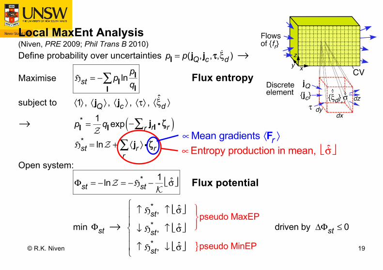
Local MaxEnt Analysis (Niven, PRE 2009; Phil Trans B 2010)

Define probability over uncertainties pI = p(jQ, jc ,τ,ξd ) →

Maximise Hst = − pI ln

pIqII

∑ Flux entropy

subject to ⟨1⟩ , ⟨jQ ⟩ , ⟨jc ⟩ , ⟨τ⟩ , ⟨ξ̂d ⟩

→ pI

* = 1Z

qI exp − jrI i ζrr∑( )

Hst

* = lnZ + ⟨jr ⟩ i ζrr∑

Open system:

Φst = − lnZ = −Hst

* − 1K

σ̂⎢⎣ ⎥⎦ Flux potential

min Φst → driven by ΔΦst ≤ 0

↑ Hst* , ↑ σ̂⎢⎣ ⎥⎦

↓ Hst* , ↑ σ̂⎢⎣ ⎥⎦

↑ Hst* , ↓ σ̂⎢⎣ ⎥⎦

⎧

⎨

⎪⎪

⎩

⎪⎪

⎫⎬⎪

⎭⎪pseudo MaxEP

}pseudo MinEP

∝Entropy production in mean, σ̂⎢⎣ ⎥⎦ ∝Mean gradients ⟨Fr ⟩

© R.K. Niven 20

Summary: MaxEnt analysis of local flow system → 1. “Minimum flux potential” principle:

Φst= −Hst

* − 1K

σ̂⎢⎣ ⎥⎦

2. Connected to subsidiary MaxEP or MinEP principles (analogous to min or max enthalpy principles)

EP in the mean

© R.K. Niven 21

MaxEnt and Dynamical Systems

© R.K. Niven 22

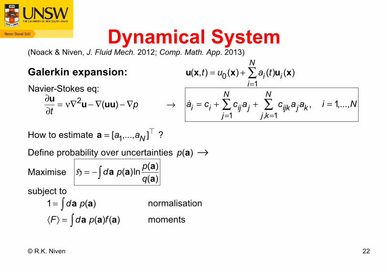
Dynamical System (Noack & Niven, J. Fluid Mech. 2012; Comp. Math. App. 2013)

Galerkin expansion: u(x,t) = u0(x) + ai (t)ui (x)

i=1

N∑

∂u∂t

= ν∇2u− ∇(uu) − ∇p → ai = ci + cijaj

j=1

N∑ + cijkajak

j,k=1

N∑ , i = 1,...,N

How to estimate a = [a1,...,aN ] ?

Define probability over uncertainties p(a) →

Maximise H = − da p(a)ln p(a)

q(a)∫

subject to 1= da p(a)∫ normalisation

⟨F⟩ = da p(a)f (a)∫ moments

Navier-Stokes eq:

© R.K. Niven 23

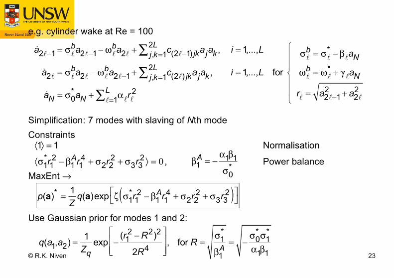
e.g. cylinder wake at Re = 100

a2 −1 = σba2 −1− ωba2 + c(2 −1) jkajakj,k=1

2L∑ , i = 1,...,L

a2 = σba2 − ωba2 −1+ c(2 ) jkajakj,k=12L∑ , i = 1,...,L

aN = σ0* aN + α r 2

=1L∑

for

σb = σ* − β aN

ωb = ω* + γ aN

r = a2 −12 + a2

2

⎧

⎨

⎪⎪

⎩

⎪⎪

Simplification: 7 modes with slaving of Nth mode Constraints ⟨1⟩ = 1 Normalisation

⟨σ1*r1

2 − β1Ar1

4 + σ2r22 + σ3r3

2 ⟩ = 0 , Power balance MaxEnt →

p(a)* = 1

Zq(a)exp ζ σ1

*r12 − β1

Ar14 + σ2r2

2 + σ3r32( )⎡

⎣⎤⎦

Use Gaussian prior for modes 1 and 2:

q(a1,a2) = 1

Zqexp −

(r12 −R2)2

2R4

⎡

⎣⎢⎢

⎤

⎦⎥⎥, for R =

σ1*

β1A

= −σ0

*σ1*

α1β1

β1

A = −α1β1σ0

*

© R.K. Niven 24

Summary: apply MaxEnt → closely match DNS solution → system closure ! Current work: - examine higher dimensionality systems (→ turbulence!)

© R.K. Niven 25

MaxEnt Analysis of Flow Networks

© R.K. Niven 26

Flow Network Consider generalised flow network, with nodes connected by flow paths:

Many applications ! - electrical, fluid flow, communications networks - transport (road, air, shipping), chemical reaction, ecological networks - human industrial, economic, social, political networks

© R.K. Niven 27

Network Specification Network structure

- N nodes, M edges - adjacency matrix A

Flow parameters - internal flow rates

Qij ∈Q (edges)

- external flow rates θi ∈ΘΘ (nodes) - potential differences

ΔEij ∈ΔE (edges) (for Δ = init − final )

Kirchhoff’s Laws

Ki ∈K : Continuity at each node i: θi − Qij

i=1

N∑ = 0

K ∈L : No potential difference around each loop :

ΔEijij∈∑ = 0

⎫⎬⎭⇒ L loops

© R.K. Niven 28

Resistance Functions Specify

ΔEij = Rij (Qij ) ∈ ΔE = R (Q )

e.g.

Electrical: linear: ΔE = RQ c.f. V = RI

Pipe flows: quadratic: ΔE = RQ2

power law: ΔE = RQ |Q |a−1 a ∈[0,1]

Colebrook:

ΔE = 8fL

π2D5gQ |Q | with

Re = 4ρQ

πμD and

f = 64|Re|

, Re < 2100

1f= 1.14 − 2.0 log10

εD

+ 9.28|Re | f

⎛⎝⎜

⎞⎠⎟, Re ≥ 4000

⎧

⎨

⎪⎪

⎩

⎪⎪

Transport: ΔE = R(Q) with ΔE →∞ as Q →Qmax

© R.K. Niven 29

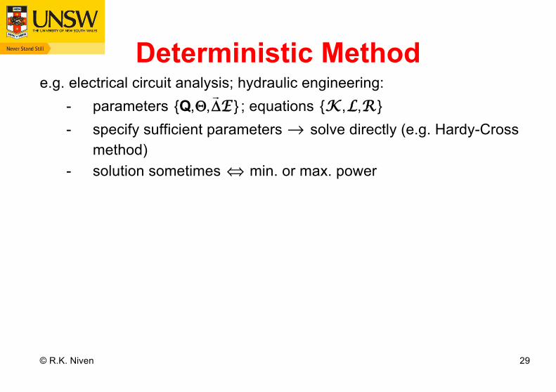
Deterministic Method e.g. electrical circuit analysis; hydraulic engineering: - parameters {Q,Θ,ΔE } ; equations {K ,L,R } - specify sufficient parameters → solve directly (e.g. Hardy-Cross

method) - solution sometimes ⇔ min. or max. power

© R.K. Niven 30

Previous Use of MaxEnt (a) Transport networks e.g. Ortúzar & Willumsen (2001): “gravity model”:

- define over trip counts Tij

→ max

H = − (Tij logTij −Tij )

ij∑

subject to Kirchhoff node constraints + cost function - use multiplier as fitting parameter

(b) Hydraulic networks e.g. Awumah et al. 1990; Tanyimboh & Templeman 1993; de Schaetzen et al. 2000; Formiga

et al. 2003, Ang & Jowitt 2003; Setiadi et al. 2005

- define probabilities

pij = Qij Qij

ij∑

→ MaxEnt subject to Kirchhoff node constraints - did not include Kirchhoff loop constraints or pipe resistances!

© R.K. Niven 31

“Standard Problem” Define probability over uncertainties → joint pdf p(Q ,Θ,ΔE )

→ maximise

Hnet = − ...∫ dQ dΘdΔE p(Q ,Θ,ΔE ) ln p(Q ,Θ,ΔE )

q(Q ,Θ,ΔE )∫

Constraints: - normalisation ⟨1⟩ - known moments: some of

⟨Qij ⟩ , ⟨θi ⟩ ,

⟨ΔEij ⟩ - resistance functions ⟨ΔE ⟩ −R (⟨Q ⟩) = 0 - Kirchhoff node + loop constraints f(⟨Q ⟩,⟨ΘΘ⟩) = 0, g(⟨ΔE ⟩) = 0

→ Boltzmann distribution, MaxEnt:

p* = qZ

exp −λλ :Q − μ iΘ − νν : ΔE − ρρ : ⟨ΔE ⟩ −R (⟨Q ⟩)( )− αα i f − ββ i g⎡⎣ ⎤⎦

Hnet* = − lnZ + λ : ⟨Q ⟩ + μ i ⟨ΘΘ⟩ + ν : ⟨ΔE ⟩

Entropy production σnet⎢⎣ ⎥⎦

Non-linearities!

© R.K. Niven 32

Comments 1. Kirchhoff constraints imposed in mean:

θi − Qij

i=1

N∑ = 0 , all nodes;

ΔEijij∈∑ = 0 , all indep. loops

2. Handling of resistance functions: I.

⟨ΔEij ⟩ = ⟨Rij (Qij )⟩ → simple Lagrangian

II. ⟨ΔEij ⟩ = Rij (⟨Qij ⟩) → implicit Lagrangian

3. Dimensionality of integrals

...∫ dQ dΘdΔE ...∫ R (Q )⎯ →⎯⎯⎯ ...∫ dQ dΘ...∫

4. Prior probabilities - Gaussian priors convenient

© R.K. Niven 33

Results 3-node network (Waldrip et al., MaxEnt2013) - 6 parameters (

⟨ΔEij ⟩ dependent)

- 3 x Ki + 1 x K - power-law resistances:

⟨ΔEij ⟩ = Kij ⟨Qij ⟩ | ⟨Qij ⟩ |

- Gaussian priors Solved numerically (multidimensional quadrature, quasi-Newton iteration for multipliers, outer implicit iteration)

Constraints ⟨θ1⟩ = 1, ⟨θ2⟩ = 0; fixed K12 = K23 = 0.5

Constraints ⟨θ1⟩ = 1; fixed K12 = K23 = 0.5

© R.K. Niven 36

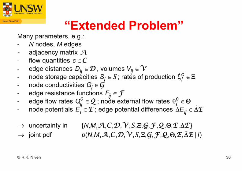
“Extended Problem” Many parameters, e.g.: - N nodes, M edges - adjacency matrix A - flow quantities c ∈C - edge distances

Dij ∈D , volumes

Vij ∈V

- node storage capacities Si ∈S ; rates of production ξic ∈ΞΞ

- node conductivities Gi ∈G - edge resistance functions

Fij ∈F

- edge flow rates Qij

c ∈Q ; node external flow rates θic ∈ΘΘ

- node potentials Ei ∈E ; edge potential differences ΔEij ∈ΔE

→ uncertainty in {N,M,A,C ,D,V ,S,Ξ,G,F ,Q ,Θ,E ,ΔE } → joint pdf p(N,M,A,C ,D,V ,S,Ξ,G,F ,Q ,Θ,E ,ΔE | I)

© R.K. Niven 37

Define probability over the uncertainties → relative entropy

Hnet = − ...∫ dX p(X | I) ln p(X | I)

q(X | I)∫ X = uncertain parameter(s)I = known information

Maximise subject to constraints → infer p(X | I) * → moments ⟨Xij ⟩

Open systems: minimise potential

Φnet = −Hnet

* − 1K

σnet⎢⎣ ⎥⎦

© R.K. Niven 38

Chemical Reaction Networks Species

X =

PQAP *QA

P+QA−

⎡

⎣

⎢⎢⎢⎢

⎤

⎦

⎥⎥⎥⎥

=XYZ

⎡

⎣

⎢⎢⎢

⎤

⎦

⎥⎥⎥

Reactions

Π = L+ L− D+ D− B1

+ B1− B2

+ B2−⎡

⎣⎤⎦

Stoichiometric matrix:

Γ =-1 1 1 -1 0 0 1 -11 -1 -1 1 -1 1 0 00 0 0 0 1 -1 -1 1

⎡

⎣

⎢⎢⎢

⎤

⎦

⎥⎥⎥

(e.g. Juretic & Županovic, 2003)

© R.K. Niven 39

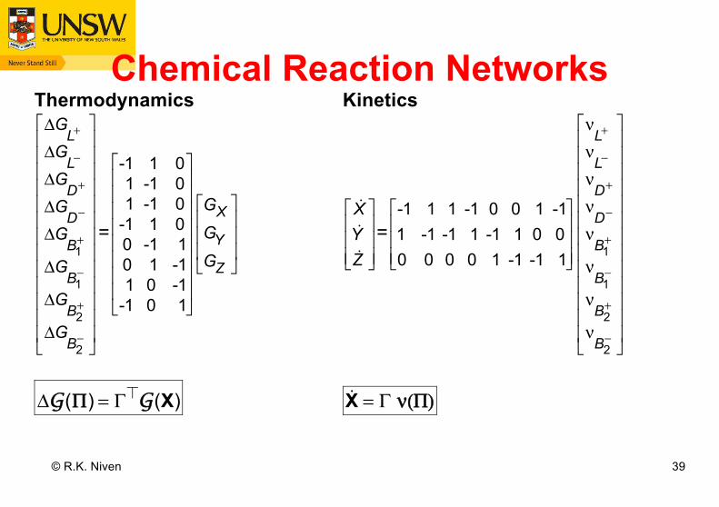
Chemical Reaction Networks Thermodynamics Kinetics

ΔGL+

ΔGL−

ΔGD+

ΔGD−

ΔGB1+

ΔGB1−

ΔGB2+

ΔGB2−

⎡

⎣

⎢⎢⎢⎢⎢⎢⎢⎢⎢⎢⎢⎢⎢

⎤

⎦

⎥⎥⎥⎥⎥⎥⎥⎥⎥⎥⎥⎥⎥

=

-1 1 01 -1 01 -1 0

-1 1 00 -1 10 1 -11 0 -1

-1 0 1

⎡

⎣

⎢⎢⎢⎢⎢⎢⎢⎢

⎤

⎦

⎥⎥⎥⎥⎥⎥⎥⎥

GXGYGZ

⎡

⎣

⎢⎢⎢

⎤

⎦

⎥⎥⎥

XYZ

⎡

⎣

⎢⎢⎢

⎤

⎦

⎥⎥⎥=

-1 1 1 -1 0 0 1 -11 -1 -1 1 -1 1 0 00 0 0 0 1 -1 -1 1

⎡

⎣

⎢⎢⎢

⎤

⎦

⎥⎥⎥

νL+

νL−

νD+

νD−

νB1+

νB1−

νB2+

νB2−

⎡

⎣

⎢⎢⎢⎢⎢⎢⎢⎢⎢⎢⎢⎢⎢

⎤

⎦

⎥⎥⎥⎥⎥⎥⎥⎥⎥⎥⎥⎥⎥

ΔG(Π) = Γ G(X) X = Γ ν(Π)

© R.K. Niven 44

Conclusions 1. MaxEnt analysis

- justification; mathematical structure

2. MaxEnt in fluid mechanics- infinitesimal fluid element

3. MaxEnt in dynamical systems- oscillatory cylinder wake

4. MaxEnt analyses of flow networks- “standard” problem: flow rates + potentials

- e.g. pipe flow system (nonlinear) - real example

- “extended” problem: further uncertainties - incl. network structure - chemical reaction networks → stationary states

model reduction of flow systems and networks by the ... · robert k. niven unsw canberra, act,...

Documents