model scenarios of shoreline change at kaanapali … resolved. thus effort is needed to observe and,...

1

MODEL SCENERIOS OF SHORELINE CHANGE AT KAANAPALI BEACH, MAUI, HAWAII: SEASONAL AND EXTREME EVENTS Sean Vitousek1, Charles H. Fletcher1, Mark A. Merrifield2, Geno Pawlak3, Curt D. Storlazzi4. 1: Department of Geology and Geophysics, 1680 East-West Rd. POST Room 721, Honolulu, Hawaii, 96822, USA. [email protected] and [email protected]. 2: Department of Oceanography, 1000 Pope Road, MSB 317, Honolulu, HI 96822,USA. [email protected]. 3: Department of Ocean Resource Engineering, 2540 Dole St., Holmes Hall 404, Honolulu, Hawaii 96822,USA. [email protected]. 4. USGS Pacific Science Center 400 Natural Bridges Drive Santa Cruz, CA, 95060, USA. [email protected]. Abstract: Kaanapali beach is a well-defined littoral cell of carbonate sand extending 2 km south from Black Rock (a basalt headland) to Hanakao’o Point. The beach experiences dynamic seasonal shoreline change forced by longshore transport from two dominant swell regimes. In summer, south swells (Hs = 1-2 m Tp = 14-25 s) drive sand to the north, while in winter, north swells (Hs = 5-8 m Tp = 14-20 s) drive sand to the south where it accumulates on a submerged fossil reef. The Delft3D modeling system accurately predicts directly observed tidal currents and wave heights around West Maui, and is applied to simulate shoreline change. Morphologic simulations qualitatively resolve the observed seasonal behavior.

INTRODUCTION Numerical modeling allows for simulations of coastal behavior provided that physical processes involved in sediment transport and morphologic development are well

Coastal Sediments '07 © 2007 ASCE

2

resolved. Thus effort is needed to observe and, through modeling, reproduce wave and current fields with adequate spatial resolution. The Delft3D modeling system accurately reproduces hydrodynamic behavior at a number of field sites (Elias et al. 2000; Klein et al. 2001; Luijendijk 2001; Walstra et al. 2001, 2003). Delft3D also reproduces observed sediment transport patterns in laboratory tests and morphologic simulations (Lesser 2000; Lesser et. al. 2004; Elias 2006) using the Van Rijn 1993 transport formulations. As an extension of these successes, it is hoped that adequate resolution of water levels, waves, and currents allow the model to reproduce sediment transport patterns in carbonate reef environments.

Kaanapali Kaanapali Beach, located on the west coast of Maui, Hawaii, lies within a well-defined littoral cell extending 2 km south from Black Rock (a basalt headland) to Hanakao’o Point. Kaanapali Beach is at the center of the Maui Nui complex shown in Figure 1, which consists of the islands of Molokai, Lanai, Maui, and Kahoolawe. Shadowed by these islands, Kaanapali is exposed to direct swell from limited windows: north (350-10o), south (210-170o), west (280-260o), as well as refracted swell from the remaining directions.

Figure 1 –Hawaiian Islands, Maui Nui, and Kaanapali.

Like the wave field, the Maui Nui current field is also spatially complex due to mean flows through the Pailolo Channel, which have been investigated in (Flament et al. 1996; Sun 1996; Storlazzi et al. 2006). Eversole (2003) characterized Kaanapali as an alongshore system that transports approximately 30,000 m3 of sand to the north during summer months driven by south swell, which later returns to the south in winter months forced by north swell. This volume of sand can result in dramatic beach width changes of more than 50 m.

Erosion Event In early July 2003, Kaanapali experienced a rapid-onset erosion event that undermined resort landscaping and infrastructure landward of Hanakao’o Point. This event was likely the result of unusually high sea levels resulting from a series of


3

mesoscale eddies that arrived over spring and summer months as seasonal sea level increased due to water column warming. Mesoscale eddies, investigated in Firing et al. (2004), can persist for weeks to months and produce sea levels 15-20 cm above normal. The Kahului tide station on Maui reached its highest recorded hourly water levels during the mesoscale eddy sequence of 2003. While 15-20 cm may seem like a small sea-level signal, in micro-tidal areas such as Hawaii (tide range = 0.6-0.8 m), these eddies represent a significant percentage of the tide range, and a significant increase on sandy shorelines otherwise exposed to nearly constant water levels. It is unlikely that the sea-level signal produced by these events would be able, by themselves, to cause significant erosion. However, when these coincide with spring tides and swell, the conditions for significant erosion exist. Mesoscale eddies are an episodic phenomenon today that represent a future permanent condition in coming decades due to eustatic sea-level rise on the order of 3 mm/year. South swell associated with the July eddy in 2003 reached a significant wave height of only 0.75 m at 10 m water depth (Tp = 15 s, breaking wave height = 1.3 m), which is considerably lower than the annually recurring deep-water significant wave height of 2 m (Tp = 17 sec, breaking wave height = 2 m). These factors emphasize the importance of sea level as a contributing factor to erosion, and seem to be a clear case of unprecedented water levels in combination with uneventful waves leading to unprecedented erosion.

Seasonal Change Seasonal profile changes at Kaanapali beach are pronounced. Accretion periods can be idealized as two simple, different systems: accretion updrift of a headland (acting as a barrier to longshore transport, similar to a groin) and accretion on a flat fossil reef. Accretion updrift of a groin has been widely studied and is a common occurrence on coastlines in the US and abroad. The case of sand accretion on a perched beach is much less common, receiving only limited scientific attention. Beach widening at Hanakao’o Point during winter months is an acute example of accretion on a perched beach, and poses one of the most interesting questions presented by the dynamic cycle of accretion and erosion at Kaanapali. Accretion at Hanakao’o is much more concentrated and dramatic than at Black Rock, even though the north end has an obvious accretion mechanism in place: the physical barrier of Black Rock. It is likely that the shallow, rough reef at Hanakao’o slows southward propagating alongshore currents generated by north swell leading to bed deposition. Hanakao’o also marks the point where swell regimes change from surging breakers in the northern portion of the beach at Black Rock where swash transport may play an important role in beach morphology to offshore dissipative breakers on the reef (characterizing the southern portion of the beach). Because of the difference in offshore depth and wave breaking characteristics, Hanakao’o likely marks the termination of swash zone transport. Improving an understanding of the various


4

processes governing beach dynamics is critical to defining the role of eddy-generated water-level changes in episodic erosion.

METHODS

Data An array of instruments shown in Figure 2 (including CTD/OBS and ADCP’s) was deployed at the 10 m depth contour along West Maui in 2003 as part of the USGS coral reef project to monitor physical processes affecting formation and lifespan of coral reef systems (Storlazzi et al., 2006). Another instrument (PUV) was deployed at Kaanapali in the summer of 2006 for further monitoring of waves and currents in shallow water.

Modeling The Delft3D-FLOW module (v. 3.24.03 used here) solves the unsteady shallow-water equations with the hydrostatic and Boussinesq assumptions. In 2D mode the model solves two horizontal momentum equations (see Eq. 1-2), a continuity equation (Eq. 3) and a transport (advection-diffusion) equation (Eq. 4) shown below:

2 2

2 2( ) 0( ) ( )

bx xe

w w

Fu u u u uu v g fvt x y x h h x y

τη νρ η ρ η

∂ ∂ ∂ ∂ ∂ ∂+ + + − + − − + =∂ ∂ ∂ ∂ + + ∂ ∂

(1)

2 2

2 2( ) 0( ) ( )

by ye

w w

Fv v v v vu v g fut x y y h h x y

τη νρ η ρ η

∂ ∂ ∂ ∂ ∂ ∂+ + + − + − − + =∂ ∂ ∂ ∂ + + ∂ ∂

(2)

[( ) ] [( ) ] 0h u h vu vt x yη η η∂ ∂ + ∂ ++ + =

∂ ∂ ∂ (3)

[ ] [ ] [ ]H H

hc huc hvc c ch D Dt x y x x y y

⎡ ⎤⎛ ⎞∂ ∂ ∂ ∂ ∂ ∂ ∂⎛ ⎞+ + = +⎢ ⎥⎜ ⎟⎜ ⎟∂ ∂ ∂ ∂ ∂ ∂ ∂⎝ ⎠ ⎝ ⎠⎣ ⎦ (4)

where u and v = the horizontal velocities in the x and y directions respectively; t = time; g = gravity; η = free surface height; h = water depth; f = coriolis force; wρ = density of water; bτ = bed friction; F = external forces due to wind and waves, eν = horizontal eddy viscosity; HD = horizontal eddy diffusivity; and c = concentration of suspended sediment. The equations are solved on a staggered finite difference grid using the Alternating Direction Implicit (ADI) method after Stelling (1984).

Computational Grids The computations of Delft3D are performed on orthogonal curvelinear grids shown in Figure 2. Modeling for this project involves two flow grids: a regional model covering the West Maui coast and a local Kaanapali model. These grids are linked either by domain decomposition (DD) or interpolation of boundary conditions from the regional grid to the local grid. The use of DD models is very elegant, although primarily used here to validate the flow field in the smaller models, and justify the use of the local grid by itself. The use of just a local grid for simulations offers an


5

improvement in computation time over domain decomposition models, especially if the single domain models return results similar to the DD models.

Figure 2 - Instrument locations and grid layout.

Boundary Conditions West Maui experiences a propagating tide, where gradient phases and amplitudes of tidal constituents exist along the coast, and tidal velocities are directed shore parallel (Storlazzi et al., 2006). Boundary conditions ideal for modeling this particular tidal configuration have been expressed in Roelvink and Walstra (2004), using water-level boundaries at the open (offshore) boundary and water-level gradient (Neumann) boundary conditions at lateral boundaries to solve for alongshore tidal velocities. The boundaries use a harmonic forcing type, which facilitates use of the harmonic tidal components in water-level boundaries and determining water-level gradients. Water-level gradient boundary conditions can be determined simply from the amplitudes and phases of the tidal constitutes at each lateral boundary using the equations given in Roelvink and Walstra (2004):

Given tidal constituent Gradient amplitude:

Amplitude: iη north southi i

itsd

φ φη⎛ ⎞−⎜ ⎟⎝ ⎠

(5)

Phase: iφ / 2iφ π+ (6)


6

where iη = amplitude of the tidal constituent (m); iφ = phase of the tidal constituent ( ,north south

i iφ φ for north and south boundaries respectively (radians)) and tsd = distance between the lateral boundaries (m). With these boundary conditions prescribed, the bed roughness is tuned to match the observed current magnitude. These boundary conditions have been shown to provide accurate simulations of tidal velocities in Roelvink and Walstra’s modeling studies (2004) at Egmond (Netherlands). This study provides another example of the excellent performance of boundary conditions developed from this scheme (see Results). The wave boundary conditions are determined from model hindcasts (WaveWatch III) because there are no recorded buoy observations that include wave direction. These hindcasts adequately resolve observed wave heights and periods at a number of buoy locations in Hawaii. In this study, hindcast values of significant wave height, peak period and direction are applied uniformly at the open boundaries of the largest SWAN model, and a series of nested grids resolve the wave field down to the nearshore scale (10m grid) at West Maui and Kaanapali Beach. The SWAN nesting scheme is shown on Figure 3.

Figure 3 - SWAN nesting scheme. WaveWatch III hindcast locations are shown in

boxes.

RESULTS Model calibration has been carried out with the USGS data set. The model shows good comparison to the observed data set for tidal water levels, wave heights, and currents. Good comparisons of tidal water levels are readily achieved with the use of a water-level boundary at the open boundary. The modeled and observed tidal components at the instrument location are shown in Table 1.


7

Table 1 - Observed vs. modeled tidal constituents at instrument locations______ Airport Honokowai Obs Amp

[m] Mod Amp [m]

Obs Phase [deg]

Mod Phase [deg]

Obs Amp [m]

Mod Amp [m]

Obs Phase [deg]

Mod Phase [deg]

M2 0.175 0.173 -124.1 -124.0 M2 0.176 0.174 -122.6 -121.6 N2 0.029 0.029 157.9 157.7 N2 0.029 0.029 159.1 160.3 S2 0.062 0.061 79.4 79.4 S2 0.061 0.06 81.2 82.1 K1 0.182 0.181 79.4 79.2 K1 0.18 0.18 79.0 78.6 P1 0.048 0.048 85.9 85.1 P1 0.048 0.048 86.3 85.3 O1 0.105 0.105 -148.2 -148.5 O1 0.105 0.104 -148.5 -148.9 K2 0.029 0.028 -107.5 -108.3 K2 0.028 0.028 -107.1 -106.6 Black Rock Puamana Obs Amp

[m] Mod Amp [m]

Obs Phase [deg]

Mod Phase [deg]

Obs Amp [m]

Mod Amp [m]

Obs Phase [deg]

Mod Phase [deg]

M2 0.177 0.174 -119.3 -118.3 M2 0.179 0.177 -107.4 -106.8 N2 0.029 0.029 161.1 163.6 N2 0.028 0.029 174.4 175.8 S2 0.059 0.058 85.3 86.0 S2 0.052 0.052 100.0 100.6 K1 0.178 0.177 78.9 77.7 K1 0.168 0.169 75.0 74.9 P1 0.048 0.047 86.9 85.2 P1 0.045 0.045 84.4 85.0 O1 0.104 0.102 -148.3 -149.3 O1 0.096 0.096 -150.8 -150.9 K2 0.027 0.027 -106.3 -103.7 K2 0.025 0.025 -95.4 -93.4 Agreement between modeled and observed currents is more difficult to achieve because of unresolved current-generating sources including mean flows through the Pailolo channel, internal tides, and the influence of the mesoscale eddy. Nevertheless the model shows good comparison with the observed currents, especially for stations dominated by barotropic flow, shown in Figure 4 and Figure 5.

Figure 4 - Modeled vs. observed current comparison for Honokowai station.


8

Figure 5 - Modeled vs. observed current comparison for the South Kahana (Airport)

station.

Use of the SWAN model appears to resolve spatial variability around and inside of the Maui Nui complex. Modeled wave heights show good comparison with observations at instrument locations shown in Figure 6. Tidal residuals from two dominant swell regimes are shown in Figure 7, which show significant longshore currents at Kaanapali. Morphologic simulations under dominant north and south swell conditions are shown in Figure 8 with aerial photographs of the seasonal beach states when these swell regimes dominate.


9

Figure 6 - WaveWatch III boundary conditions and comparisons of modeled (x) and

observed (-) wave heights [m] at instrument locations. The lines on the second subplot represent the south swell window (170-210o).

Figure 7 - Tidal residuals [m/s] for South (A) and North (B) swell at Kaanapali Beach

A B


10

Figure 8 – Observed (above) and simulated (below) beach states (accretion - red;

erosion - blue [m]) during summer (left) and winter (right) swell conditions.

DISCUSSION Using Delft3D with water-level gradient boundary conditions prescribed in Roelvink and Walstra (2004) provide excellent resolution of current velocities in regions dominated by barotropic tidal flow. For regions influenced by mean flows and internal tides, more physical processes need to be accounted for to better resolve observed velocities. It appears the Honokowai station (Figure 4) is well resolved, while the South Kahana (Airport) station (Figure 5) is influenced by the presence of mean flows and internal tides. Despite the influence of unresolved processes, the models show good comparison with the observed flow velocities.


11

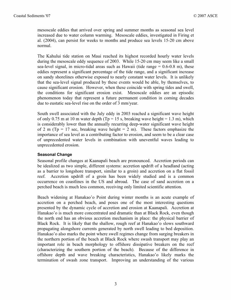
Mean flows observed at the South Kahana (Airport) Station appear to be related to wind direction, and may be related to island-trapped wave events (Merrifield 2002; Storlazzi 2006). Figure 9 shows the time series of wind speed and mean flow and their inter-relationship.

Figure 9 - Relationship between winds and mean flow through the Pailolo Channel.

Wind speed and mean flow seem to mirror each other. A notable event in the time series is the decrease in wind speed in late July which leads to a corresponding decrease in the mean flow through the channel. Although the model accounts for wind forcing, the mean flow is not resolved. If the mean flow is due to wind forcing, the inability to resolve the mean flow is probably due to the limited coverage of the model domain: inability to develop significant wind-generated currents, and/or the topographic influence of West Maui which may cause local acceleration of the wind field. The mean flow observed at South Kahana seems unlikely, from the two observed time series, to extend past the Honokowai station and potentially affect currents and sand transport at Kaanapali Beach. The major influence in sand transport at Kaanapali seems to be the wave-generated currents that arise from obliquely incident waves from north and south swell breaking on the westward-facing shoreline. While simulations of shoreline accretion and erosion forced by the dominant swell regimes show a qualitative morphologic behavior, the ultimate goal of modeling is to reproduce or predict transport volumes and resulting changes in the beach profile. Modeling beach profile changes often captures observed changes in mean state, but is


12

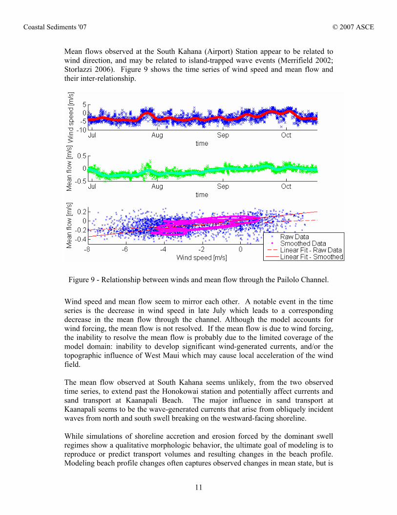
less successful at predicting significant erosion and accretion events. While the model seems to perform adequately for scenarios on timescales of a few days, variability of wave and current conditions on longer timescales make simulations on timescales of months to years more difficult to resolve. Comparisons of observed and modeled profile changes, in Figure 10, show that the model tends to overpredict accretion (indicated by the frequency of records in quadrant 2 and above the perfect fit line) and to miss large erosion and accretion events in the end members of the littoral cell (Black Rock and Hanakao’o). Bias towards accretion is likely due to the persistence of small wave states during the 3-month simulation, and inability to resolve swell events that lead to significant change. The effects of 2D vs. 3D modeling on accretion predictions should also be investigated.

Figure 10 - Observed vs. modeled beach profile changes over 3 months at a number

of locations at Kaanapali, Summer 2000.

Additionally, there appears to be no significant difference in modeling the summer 2003 erosion event with and without the presence of the small sea-level signal contributed by mesoscale eddies. This is likely the result of discretization by the model. There is an inherent problem simulating natural processes using discrete numerical simulations, especially when variability of a particular process, in this case sea level in its vertical and horizontal position, exists on a smaller scale than the discrete grid is capable of resolving. Another process we are not effectively resolving in the model is the action of swash transport producing morphologic changes in the beach face. The model does, however, have a scheme to replicate morphologic beach face changes by applying a relative amount of erosion or accretion in wet grid cells to


13

adjacent dry grid cells. While this scheme is a practical solution to an extremely complex problem, it does leave a potentially important processes unresolved. We can, however, make interesting conclusions about sand transport from simulations of simple scenarios. Morphologic simulations of transport due to north swell with a uniform bed roughness demonstrate transport of a considerable amount of sand around Hanakao’o Point. Increasing the simulated roughness for the submerged fossil reef offshore from Hanakao’o Point causes the sand to accumulate in this location. This is consistent with field observations. Inability of the model to resolve the signal of the mesoscale eddy should not cause us to dismiss its influence. Simple Bruunian models assign sea-level position paramount influence, although the presence of reef surfaces may change this simple dynamic. It appears that increased sea level on a normal shoreline profile (not perched) may exist in unstable equilibrium until wave energy initiates transfer to a new position. The duration of mesoscale eddies is sufficient to begin this transition as evidenced by the considerable erosion observed in summer 2003 at Kaanapali. The event also suggests that increased sea-level signals may cause accelerated seasonal response in alongshore systems. CONCLUSIONS Robust numerical models allow for realistic shoreline change simulations. Adequate observations are indispensable to ensure realistic performance. Poor modeling performance arises from inadequate tuning, unresolved processes, and spatial discretization of continuous natural processes. Use of water-level gradient boundary conditions given by observations of tidal components and the equations used in Roelvink and Walstra (2004) successfully model tidal velocities. Scenario-based modeling of seasonal shoreline change is qualitatively successful, whereas real-time, long-term simulations often to not capture significant changes in beach profile and shoreline position. Mesoscale eddies and accretion on perched beaches atop rough reef substrates play a potentially significant role in beach morphology of Hawaiian shorelines, and merit continued investigation. ACKNOWLEDGMENTS The authors would like to thank Edwin Elias, Dolan Eversole, Chris Conger, Jeff List, Capt. Joe Reich, Lamber Hulsen, Dano Roelvink, Dirk-Jan Walstra, Everyone at Delft3D support: Johan Dijkzeul, Arjen Luijendijk, and Meo de Rover. This paper is funded by a grant/cooperative agreement from the National Oceanic and Atmospheric Administration, Project # R/EP-26, which is sponsored by the University of Hawaii Sea Grant College Program, SOEST, under Institutional Grant No. NA05OAR4171048 from NOAA Office of Sea Grant, Department of Commerce. The views expressed herein are those of the author(s) and do not necessarily reflect the views of NOAA or any of its subagencies. UNIHI-SEAGRANT-OP-07-06.


14

REFERENCES: Elias, W.P.L. (2000). “Hydrodynamic validation of Delft2/3D with field measurements at

Edmond,” Proc. 27th ICCE, Sydney, Australia. Elias, W.P.L. (2006). “Morphodynamics of Texel Inlet,” Ph. D. thesis. Delft University of

Technology, The Netherlands. Eversole, D., Fletcher, C.H., (2003). “Longshore Sediment Transport Rates on a Reef-

Fronted Beach: Field Data and Empirical Models Kaanapali Beach, Hawaii,” Journal of Coastal Research: Vol. 19, No. 3, pp. 649–663.

Firing, Y. L., and Merrifield, M. A., (2004). “Extreme sea level events at Hawaii: Influence of mesoscale eddies,” Geophys. Res. Lett. 31, L24306

Flament, P., Lumpkin, C., (1996). “Observations of currents through the Pailolo Channel: Implications for nutrient transport,” In: Wiltse, W. (Ed.), Algal Blooms: Progress Report on Scientific Research, West Maui Watershed Management Project, pp. 57 –64.

Klein, M.D., Elias, E.P.L., Stive, M.J.F., Walstra, D.J.R., (2001). “Modelling inner surf zone hydrodynamics at Egmond, The Netherlands,” In: Hanson, H., Larson, M. (Eds.), Proc. 4th Int. Conf. on Coastal Dynamics ’01. ASCE, Reston, pp. 500–509.

Lesser, G.R., (2000). “Computation of Three-dimensional Suspended Sediment Transport within the DELFT3D-FLOW Module,” Master’s thesis. Delft University of Technology, The Netherlands.

Lesser, G.R., Roelvink, J.A., van Kester, J.A.T.M., Stelling G.S., (2004). “Development and validation of a three-dimensional morphological model,” Coastal Engineering. v. 51. pp. 883–915.

Luijendijk, A.P., (2001). “Validation, calibration and evaluation of Delft3D-FLOW model with ferry measurements,” Master’s thesis. Delft University of Technology, The Netherlands.

Merrifield, M.A., Yang, L., Luther, D.S., (2002). “Numerical simulations of a storm generated island-trapped wave event at the Hawaiian Islands” Journal of Geophysical Research 107 (C10), 3169.

Roelvink, J.A., Wasltra, D.J., (2004). “Keeping in simple by using complex models,” 6th International Conference on Hydroscience and Engineering, Advances in Hydro- Science and Engineering, Brisbane, Australia.

Stelling, G.S., (1984). “On the construction of computational methods of shallow water flow problems,” Rijkswaterstaat communications, No. 35

Storlazzi, C.D., McManus, M.A., Logan, J.B. McLaughlin, B.E., (2006). “Cross-shore velocity shear, eddies and heterogeneity in water column properties over fringing coral reefs: West Maui, Hawaii,” Continental Shelf Research 26 (2006) 401 –421

Sun, L.C., (1996). “The Maui algal bloom: the role of physics,” In: Wiltse, W. (Ed.), Algal Blooms: Progress Report on Scientific Research. West Maui Watershed Management Project, pp. 54 –57.

Walstra, D.J.R., Roelvink, J.A., Groeneweg, J., (2000). “Calculation of wave-driven currents in a 3D mean flow model,” Proc. 27th Int. Conf. on Coastal Engineering. ASCE, New York, pp. 1050– 1063.

Walstra, D.J.R., Van Rijn, L.C., Boers, M., Roelvink, J.A., (2003). “Offshore sand pits: verification and application of hydrodynamic and morphodynamic models,” Proc. 5th Int. Conf. on Coastal Sediments ’03. ASCE, Reston, Virginia


model scenarios of shoreline change at kaanapali … resolved. thus effort is needed to observe and,...

Documents