Model Selection for Geostatistical Models∗

Jennifer A. Hoeting, Richard A. Davis, Andrew A. Merton

Colorado State University

Sandra E. Thompson

Pacific Northwest National Lab

August 7, 2004

Abstract

We consider the problem of model selection for geospatial data. Spatial correlation is oftenignored in the selection of explanatory variables and this can influence model selection results.For example, the inclusion or exclusion of particular explanatory variables may not be apparentwhen spatial correlation is ignored. To address this problem, we consider the Akaike InformationCriterion (AIC) as applied to a geostatistical model. We offer a heuristic derivation of the AIC inthis context and provide simulation results that show that using AIC for a geostatistical model issuperior to the often used traditional approach of ignoring spatial correlation in the selection ofexplanatory variables. These ideas are further demonstrated via a model for lizard abundance.We also employ the principle of minimum description length (MDL) to variable selection for thegeostatistical model. The effect of sampling design on the selection of explanatory covariates isalso explored. S-Plus and R software to implement the geostatistical model selection methodsdescribed in this paper is available at www.stat.colostate.edu/∼jah.

KEYWORDS: geospatial data, AIC, MDL, kriging, Matern autocorrelation function,

orange-throated whiptail lizard abundance

1 Introduction

Ecologists and scientists in other fields typically consider a number of plausible models in statistical

applications. Formal consideration of model selection in ecological applications has dramatically

increased in recent years, perhaps in part due to the publication of the book by Burnham and

Anderson (1998; 2002). Concurrently, the wide availability of inexpensive global positioning systems

and other advances in technology have allowed for the collection of vast quantities of data with

geo-referenced sample locations. As a result, models for spatially correlated data are becoming

increasingly important. We consider these two problems together, spatial modeling and model

selection. The importance of accounting for spatial correlation has been discussed in other contexts

(Cressie, 1993), but the effect of spatial correlation on model selection has not been fully explored.

∗Research supported in part by National Science Foundation grants DEB-0091961, DMS-9806243 (Hoeting), DMS-0308109 (Davis), and by STAR Research Assistance Agreement CR-829095 awarded to Colorado State University bythe U.S. Environmental Protection Agency (Hoeting and Davis). EPA does not endorse any products or commercialservices mentioned here. The views expressed here are solely those of the authors.

1

A general philosophy for choosing a model is that we would like to incorporate information that

we believe influences the response variable while acknowledging that we do not know everything

associated with the response. These unknowns could be quantities that we did not (or could not)

measure, complex variable interactions, heterogeneity, etc. Thus an error process is often included

in the model that “accounts” for these unknowns. For example, we may suspect that the abundance

of a certain species is dependent on the availability of a certain type of vegetation and the predator

to prey ratio. But we must acknowledge that other variables are likely to play an important role

such as the abundance of fresh water or the prevalence of a certain disease. Thus the model that

we construct must account for these unknown influences. This is the main role of any error term in

any such modeling exercise. The problem becomes more complicated when we consider that there

may be competing models each using a different subset of known variables. For example, perhaps

there are two types of vegetation that the species will eat. Is either vegetation species a better

predictor of abundance or perhaps some combination of the two? In other words, which subset

of explanatory variables and error structure together provides the best model? To attempt to

answer this question, we adopt a geostatistical model (Cressie, 1993) which can be used to predict

a response at unobserved locations. This approach, also referred to as kriging, involves the fitting

of an autocorrelation function which describes the relationship between observations based on the

distance between the observations. This method allows for any number of the explanatory variables

observed at the sample locations to be included in the model to improve the overall predictions.

Typically spatial correlation is ignored in the selection of explanatory variables. Ignoring the

autocorrelation structure in the data can influence model selection results. For example, the impor-

tance of particular explanatory variables may not be apparent when spatial correlation is ignored.

To address this problem, we consider the Akaike Information Criterion (AIC) as applied to a geo-

statistical model. We provide simulation results that show that using AIC for a geostatistical model

is superior to the standard approach of ignoring spatial correlation in the selection of explanatory

variables. We also consider the impact of the sampling pattern on the model selection. We further

demonstrate these ideas via a model for the abundance of the orange-throated whiptail lizard found

in southern California. The principle of minimum description length (MDL) applied to the variable

selection problem is also investigated and simulation results are provided for comparison.

Our paper proceeds as follows. In Section 2 we describe a geostatistical model and methods for

parameter estimation by using the whiptail lizard data set as a working example. In Section 3 we

develop the AIC as applied to a geostatistical model and discuss spatial model fitting and other

model selection issues. Simulation results in Section 4 and an example in Section 5 underscore

the importance of accounting for spatial correlation in the selection of explanatory variables. The

effect of sampling design on the selection of explanatory variables for geostatistical models is also

considered in Section 4. S-Plus and R software to implement the methods described in this paper

will be made freely available on the internet. In the Appendix we offer a heuristic derivation of the

2

AIC in context of the geostatistical model.

2 The Geostatistical Model

Suppose we are interested in the abundance of the orange-throated whiptail lizard in a specific

region in southern California. (Analysis results of this data set are given in Section 5.) Assume

that we have collected information at each of 150 sites spread across the area of interest. Our data

set consists of the average number of lizards observed per day, the percent coverage of vegetation,

the abundance of ants (a primary food source), and a geo-reference for each site, such as latitude

and longitude. It is not feasible to collect data at all possible locations, thus we are assuming

that these 150 sites are representative of the entire area of interest. Let Z(si) denote the average

abundance of lizards at site i where i = 1, . . . , 150. Thus the vector Z = (Z(s1), . . . , Z(s150))′ is a

partial realization of the continuous random field over this finite area, D. In other words, we are

assuming that at any given site s within the domain D, the average abundance of the lizards is a

function of a specific set of variables that can be observed along with some random noise.

A model for the continuous random field at any location s ∈ D is given by

Z(s) = β0 + β1X1(s) + . . . + βp−1Xp−1(s) + δ(s)

= X′(s)β + δ(s),

(1)

where X(s) = (1, X1(s), . . . , Xp−1(s))′ is a p vector consisting of the constant 1 and p−1 explanatory

variables observed at location s, β = (β0, . . . , βp−1)′ is a p vector of the unknown model coefficients,

and δ(s) is the unobserved “regression” error at location s. For example, X1(s) and X2(s) may

be the percent coverage of vegetation and the abundance of ants at location s, respectively. For

computational ease we will assume that the error process δ(s) is a stationary, isotropic Gaussian

process with mean zero and covariance function Cov(δ(si), δ(sj)) = σ2ρθ(||si−sj ||). Here σ2 is the

variance of the process, ρθ(|| · ||) is a family of autocorrelation functions with a parameter vector

θ of length k, and || · || denotes the Euclidean distance between two sites. Thus, we assume that

the correlation between any two sites is only a function of the distance between them. In deciding

among the covariates, we must also choose an appropriate autocorrelation function. As will be

demonstrated below, these two issues are inextricably linked.

The autocorrelation function must satisfy certain mathematical conditions in order to be valid.

This restricts our selection to one of a number of standard autocorrelation families. Most readers

should be familiar with the independent error process associated with multilinear regression. In

this case one is assuming that the errors are identically distributed and independent of one another

and location. For geospatial data, it is reasonable to assume that observations that are nearby will

have similar response values, so we seek to model this relationship via the autocorrelation function.

A rich family of autocorrelation functions is the Matern family (Handcock and Stein, 1993; Stein,

3

1999). The Matern autocorrelation function has the general form

ρθ(d) =1

2θ2−1Γ (θ2)

(

2d√

θ2

θ1

)θ2

Kθ2

(

2d√

θ2

θ1

)

, θ1 > 0, θ2 > 0, (2)

where Kθ2(·) is the modified Bessel function of order θ2 (Abramowitz and Stegun, 1965). The

“range” parameter, θ1, controls the rate of decay of the correlation between observations as dis-

tance increases. Large values of θ1 indicate that sites that are relatively far from one another are

moderately (positively) correlated. The parameter θ2 can be described as controling behavior of the

autocorrelation function for observations that are separated by small distances. The Matern class

includes the exponential autocorrelation function when θ2 = 0.5 and the Gaussian autocorrelation

function as a limiting case when θ2 → ∞. The Matern class is very flexible, being able to to strike

a balance between these two extremes, thus making it well suited for a variety of applications.

Figures 1 and 2 illustrate the flexibility of the Matern autocorrelation function. Notice that for

small distances the correlation between sites is large and decreases as distance increases.

The autocorrelation function given in (2) can be further adapted to include the possibility of

measurement error, called nugget in many spatial contexts. A mixture model that incorporates

measurement error in these spatial models is considered in Thompson (2001). To minimize the

complexity of the current discussion, we have chosen not to include a nugget effect in our simula-

tions or analysis of the lizard data example. It should be noted that selection of the form of the

autocorrelation function can be easily incorporated into the model selection process. For example,

one could assume that the autocorrelation function is Matern but allow the selection process to

determine whether or not a nugget should be included.

2.1 Estimation

The model in (1) is often referred to as a geostatistical model or a universal kriging model. For a

particular subset of explanatory variables and a structure for the error process, we are now tasked

with estimating the parameters β, σ2, and θ. Estimation of the parameters of this model can

proceed using one of several likelihood based approaches (Cressie, 1993; Haining, 1990; Smith,

2000) or a Bayesian approach (Handcock and Stein, 1993; Thompson, 2001). Here we consider the

former. Both approaches can be computationally challenging to implement for large sample sizes.

Using the assumption that the error process is Gaussian, the log-likelihood of the parameters

in equation (1),(

θ, β, σ2)

, based on the observed data, Z, is given by

ℓ(

θ, β, σ2; Z)

= −1

2log

∣

∣σ2Ω

∣

∣ − 1

2σ2(Z − Xβ)′ Ω−1 (Z − Xβ) ,

where Ω = [ρθ(||si − sj ||)] represents the matrix of correlations between all pairs of observations,

i, j = 1, . . . , n. By concentrating out β and σ2, the profile likelihood can be easily computed

which can often accelerate optimization of the likelihood. That is, by maximizing the likelihood

4

with respect to β and σ2, we obtain β = β (θ) =(

X ′Ω

−1X)

−1X ′

Ω−1Z and σ2 = σ2 (θ) =

(

Z − Xβ)

′

Ω−1

(

Z − Xβ)

/n. The resulting log profile likelihood is

ℓprofile

(

θ; β, σ2, Z)

= −1

2log |Ω| − n

2log

(

σ2)

− n

2. (3)

Maximizing (3) produces the maximum likelihood estimates for the parameters of the spatial au-

tocorrelation function, θ.

An alternative approach for parameter estimation is the restricted maximum likelihood (REML)

approach of Patterson and Thompson (1971). Cressie (1993), p.93, supports the use of REML over

maximum likelihood as a method of estimation when the number of explanatory variables is large.

For model selection, most procedures involve a component consisting of the maximized likelihood

function. Since REML does not maximize the likelihood, we do not consider REML here further.

However, once a model has been selected, the researcher is free to re-estimate the model parameters

using, for example, REML for parameter estimation.

3 Model Selection for Geostatistical Models

Model selection is a critical ingredient in nearly any model building exercise. Depending on one’s

philosophical bent, which is often driven by the modeling objective, there are a myriad of procedures

for selecting an optimal model subject to a particular criterion. The introductions in the books

by McQuarrie and Tsai (1998) and Burnham and Anderson (2002) give excellent accounts of the

various philosophies underpinning model selection. It is important, however, to adopt a model

selection paradigm that reflects the ultimate objective of the modeling process. For example, an

explanatory model that establishes useful relationships between explanatory and response variables

may not necessarily perform as well as a predictive model and vice versa. Section 3.1 develops the

Akaike Information Criterion (AIC) for spatial models of the form (1) while Section 3.2 discusses

spatial model fitting. Section 3.3 contains a brief discussion of the concept of Minimal Description

Length (MDL) and further remarks on model selection issues. (Online Appendix B gives the

formulas for all three model selection procedures described here).

Returning to our working example of the whiptail lizard, the current question at hand is which

model should be selected? Should we include both of the potential explanatory variables, just one,

or perhaps neither? What is required is a quantitative measure of how closely each of the candidate

models coincides with the true model. We may also wish to penalize less parsimonious models. We

suggest that AIC, extended to spatial models, accomplishes these goals.

3.1 AIC for Spatial Models

There are often two points of view taken in model selection. The first presumes that there exists

a true finite-dimensional model from which the data were generated. For example, one might

5

hypothesize the true model to be linear in which there exists an explicit linear relationship between

the explanatory variables and the response. In this case, the key modeling objective is to identify the

correct set of covariates that comprise the model. The second modeling perspective, which seems

particularly well suited for ecological data, is that the “truth” and consequently, the underlying true

model, is essentially infinite dimensional and we have no hope of identifying all the requisite factors

that go into the process under study. In other words, reality cannot be expressed as a simple, “true

model” because, as Burnham and Anderson (1998) observe, “[Ecological] systems are complex,

with many small effects, interactions, individual heterogeneity, and individual and environmental

covariates (being mostly unknown to us).” Thus, the goal is to find the best approximating finite

dimensional model to this infinite dimensional problem.

Under the first scenario, consistency should be a minimum requirement of a model selection

procedure. That is, as more data are acquired, the model selection procedure should ultimately

choose the correct model with probability one. In the second situation when the true model is

infinite dimensional, a model selection procedure ought to choose a finite dimensional model that

is closest to the true model in some sense. The Akaike Information Criterion (Akaike, 1973) is one

procedure that is designed to achieve this second goal.

AIC was developed as an estimator of the Kullback-Leibler Information. Roughly speaking AIC

is a measure of the loss of information incurred by fitting an incorrect model to the data. To describe

the main idea behind AIC, let Z be an n-dimensional random vector with true probability density

function fT and consider a family f(·; ψ), ψ ∈ Ψ of candidate probability density functions. The

Kullback-Leibler information between f(·; ψ) and fT is defined as

I(ψ) =

∫

−2 log

f(z; ψ)

fT (z)

fT (z)dz . (4)

Applying Jensen’s inequality, we see that

I(ψ) =

∫

−2 log

f(z; ψ)

fT (z)

fT (z)dz

≥ −2 log

∫

f(z; ψ)

fT (z)fT (z)dz

= −2 log

∫

f(z; ψ)dz

= 0 ,

with equality holding if and only if f(z; ψ) = fT (z) almost everywhere with respect to the true

model fT .

By treating I(ψ) as the information loss associated with f(·; ψ), the idea is to minimize I(ψ)

over all candidate models ψ ∈ Ψ. Unfortunately this is not possible without knowing fT , thus we

need to adopt a strategy that is not dependent on the unknown density fT .

6

First rewrite the Kullback-Leibler information in the following manner;

I(ψ) =

∫

−2 log

f(z; ψ)

fT (z)

fT (z)dz

=

∫

−2 log f(z; ψ) fT (z)dz +

∫

2 log fT (z) fT (z)dz

= ∆(ψ) +

∫

2 log fT (z) fT (z)dz.

(5)

The first term, defined as the Kullback-Leibler index, can be written as ∆(ψ) = ET −2 log LZ(ψ)where the expectation is taken with respect to the true density and LZ(ψ) is the likelihood based

on the candidate model corresponding to ψ using the data Z. Note that the second term in (5)

is a constant and plays no role in the minimization of I(ψ). While it is generally not possible

to compute either ∆(ψ) or ∆(ψ), where ψ is the maximum likelihood estimate of ψ, we instead

strive to find a model that minimizes an unbiased estimate of Eψ(∆(ψ)), where Eψ represents the

expectation operator relative to the candidate density f(·; ψ).

A heuristic derivation of the AIC statistic in the spatial model setup of (1) can be found in the

Appendix. The quantity

AICC = −2 log LZ(ψ) + 2np + k + 1

n − p − k − 2(6)

is an approximately unbiased estimate of the expected Kullback-Leibler information evaluated at ψ,

where there are p explanatory variables, including an intercept term, k is the number of parameters

associated with the autocorrelation function, and n is the number of observed sites. This version is

known as the corrected AIC (AICC) which includes a measure of the quality of fit of the model (first

term) and a penalty factor for the introduction of additional parameters into the model (second

term). The AIC statistic for this model is

AIC = −2 log LZ(ψ) + 2(p + k + 1).

For large n the penalty factors, 2n(p+k +1)/(n−p−k− 2) and 2(p+k +1) are nearly equivalent.

The AICC statistic has a more severe penalty for larger order models which helps counterbalance

the tendency of AIC to over fit models to data.

The principle of AIC is to select a combination of explanatory variables and models for the

autocorrelation function which minimize either AICC or AIC. It is worth remarking that in many

classical situations, such as linear regression or time series modeling, AICC and AIC are not con-

sistent order selection procedures. In other words, as the sample size increases there is a positive

probability that a model selected by AICC or AIC does not correspond to the true model. Nev-

ertheless, these statistics should produce good estimates of the Kullback-Leibler Information for

which they were formulated.

7

3.2 Spatial Model Fitting

Traditionally, the fitting of the model (1) is accomplished in two steps (see, for example, Venables

and Ripley (1999), p. 439–444). In the first step, explanatory variables for modeling the large

scale variation are chosen via a model selection technique such as Akaike’s Information Corrected

Criterion (AICC) (Sugiura, 1978; Hurvich and Tsai, 1989). Second, the residuals from the model

are examined for spatial correlation and a suitable family of correlations is chosen. The estimates

of the parameters in the trend surface are updated using generalized least squares followed by

maximum likelihood estimation of the parameters of the covariance function using the residuals.

This two step estimation process is repeated until some suitable convergence criterion is attained.

Since a correlation function is not identified in the selection of the explanatory variables in Step

1, AICC is implemented under the working assumption of independence of the residuals (Cressie,

1993; Haining, 1990).

A limitation of the model selection procedure described above is that it ignores potential con-

founding between explanatory variables and the correlation in the spatial noise process δ(s).Although it is extremely convenient to select explanatory variables for the model before fitting a

covariance function to the residuals, it is generally not a good idea to separate these two steps.

The inclusion of one or more important explanatory variables may remove or reduce the correlation

structure of the residuals from the model. For example, Ver Hoef et al. (2001) demonstrate the

similarities between a model with independent errors and a linearly decreasing mean and a model

with correlated errors and a constant mean. Alternatively, ignoring the autocorrelation structure of

the error process may mask explanatory variables which are very important in modeling the mean

function. The additional noise in the data can overwhelm the information in the data, resulting

in the identification of fewer important explanatory variables. An example of this behavior will be

explored in Section 4.

Model selection techniques for spatial models need to include the correlation structure in de-

termining the best set of predictors. By computing the AICC statistic described in Section 3.1 for

all possible sets of explanatory variables and autocorrelation functions, one can find a single “best”

model or a set of models which fit the data well. This method attempts to strike a balance between

the competing forces of large scale variability as modeled via the explanatory variables with small

scale variability as modeled through the correlation in the residuals.

3.3 Other considerations

In Section 3.1 the AICC statistic presented for the geostatistical model (1) required that the true

model was a member of the family of candidate models, all of which were finite dimensional.

However, in many applications (McQuarrie and Tsai, 1998; Burnham and Anderson, 2002), the

AICC selection procedure enjoys additional optimality properties regarding the choice of a finite-

8

dimensional model when the true model is in fact infinite dimensional. This includes the notion of

efficiency for prediction in time series models and optimal signal-to-noise ratios for linear models

(McQuarrie and Tsai, 1998).

AIC and other information-based criteria such as BIC and HQ (Kass and Raftery, 1995; Mc-

Quarrie and Tsai, 1998) have an objective function consisting of two pieces. The first is related to

-2(log-likelihood), which is a measure of the quality of fit of a model, and the second is a penalty

factor for the introduction of additional parameters into the model. The principle of minimum

description length (MDL), an idea developed by Rissanan in the 1980s, also contains two similar

pieces, but is motivated by different ideas. MDL attempts to achieve maximum data compression

by the fitted model.

The idea behind MDL is to decompose the code length of the “data” into two pieces (see the

survey paper by Lee (2001) for more details). Roughly speaking, the code length of the “data” is

the amount of memory required to store the data. Typically the code length of the data can be

decomposed into the sum of the code length of the fitted model and the code length of the data

given the fitted model, i.e.,

L(“data”) = L(“fitted model”) + L(“data given fitted model”).

Here L(“fitted model”) might be interpreted as the code length of the model parameters and

L(“data given fitted model”) as the code length of the residuals from the fitted model. It follows

that a more complex model is chosen provided there has been a compensating decrease in the code

length of the residuals. According to the MDL principle, the best model is the one producing

the shortest code length for the data. The attraction of this procedure is that the data is being

compressed in the most efficient manner possible and the notion of a true model at any level is not

required.

The code length of the fitted model based on the MLE, ψ, can be approximated by

L(“fitted model”) ≃ 1

2(p+k+1) log2 n. The code length of the data given the model based on ψ is

approximated by log2 L(ψ). Adding these terms together and rescaling, the minimum description

length is defined by

MDL =1

2

(

−2 log(LZ(ψ)) + log(n)(p + k + 1))

.

The only difference between the value of AICC (using the spatial AICC method) and 2·MDL is the

magnitude of the penalty term coefficient. For AICC, the leading coefficient is of order 2 compared

to log(n) for 2·MDL. For sample sizes greater than 8, the penalty for 2·MDL is larger. For example,

when n = 100, p = 4, and k = 2 the penalty coefficients are 2 and 4.60, respectively. MDL generally

selects more parsimonious models, i.e., models with fewer explanatory variables.

Bayesian model averaging is an alternative approach to model selection and prediction (Hoet-

ing et al., 1999). The idea of Bayesian model averaging is to average across several models instead

9

of selecting one model. In computing the average, each model is weighted by its posterior model

probability, a measure of the degree of model support in the data. Empirical and theoretical results

over a broad range of model classes indicate that Bayesian model averaging can provide improved

out-of-sample predictive performance as compared to single models. For the geostatistical model

in (1), Thompson (2001) showed that Bayesian model averaging can offer improved predictive per-

formance as compared to the single models that are selected when spatial correlation is ignored.

However, the gains are modest in the simulations that were explored.

4 Simulation

To explore the impact of ignoring spatial correlation on model selection, we carried out a simulation

comparing the explanatory variables selected using standard independent AIC model selection

which ignores spatial correlation to those selected using the spatial AIC approach and the MDL

approach described in Section 3. In addition to comparing the impact of accounting for spatial

correlation in the selection of a set of explanatory variables, we also explored the impact of sampling

pattern on the selection of explanatory variables. We considered five sampling patterns shown

in Figure 4; highly clustered, lightly clustered, random, regular, and a grid design. Finally, we

conducted some simulation studies to characterize the strength of the predictive ability when spatial

correlation is included in the selection process of explanatory variables.

We simulated five possible explanatory variables, X1, X2, X3, X4, X5. Each explanatory vari-

able was independently generated from a standardized Student’s t distribution with 12 degrees of

freedom, Xi ∼√

12

10t12 for i = 1, . . . , 5. The explanatory variables were fixed and identical for all

simulations.

For a given sampling pattern of size n = 100, the data were simulated from the model

Z = 2 + 0.75X1 + 0.50X2 + 0.25X3 + δ, (7)

where δ is a Gaussian random field with mean zero, σ2 = 50, and autocorrelation Matern with

parameters θ1 = 4 and θ2 = 1. (Results for other values of the Matern parameters are also

provided.) For each sampling pattern, 500 to 1000 replicates were simulated with a new Gaussian

random field generated for each replication. The largest signal of (7) is associated with X1 which

is three times the “strength” of X3. Thus we expect that the majority of models selected should

at least include X1.

With five possible explanatory variables, there are 25 = 32 possible combinations of explanatory

variables, including the intercept-only model. For each realization, we computed the AICC statistic

for all 32 possible models. For the traditional method, the AICC statistic was calculated using (6)

with k = 0. We call this the independent AICC approach. The spatial AICC results were calculated

10

Table 1: Model Selection Results for the Random Pattern. Independent AICC, Spatial AICC, and

MDL report the percentage of simulations that each model was selected. Of the 32 possible models,

the results given here include only those with 10% or more support for one of the models.

Variables in ModelSpatial

AICC

Independent

AICCMDL

X1, X2, X3 56.0 2.4 40.4

X1, X2, X3, X5 14.4 0.2 4.2

X1, X2, X3, X4 10.8 0.2 0.8

X1, X2 10.2 8.4 46.4

Intercept only 0.0 26.8 0.0

X1 0.4 14.2 1.2

X2 0.0 13.8 0.2

using (6) as well with k = 2. Further details on the simulation set-up and additional simulation

results are given in Thompson (2001).

4.1 General Simulation Results

Table 1 compares the models selected by the spatial AICC and independent AICC approaches.

When independence is assumed, the AICC statistic selects the true model (X1, X2, X3) only 12

out of 500 simulations (2.4%) while the intercept-only model is selected in 134 out of 500 simulations

(26.8%). Over all 500 simulations, the AICC independence approach selected models that included

both explanatory variables X1 and X2 only 15.8% of the time. These results provide a vivid

example of the drawbacks of the standard model selection approach for spatially correlated data.

In total, the first explanatory variable is in 40.2% of the selected models, and the second explanatory

variable is included in 35.4% of the models.

Spatial AICC has superior model selection performance as compared to the independent AICC

method. The true model is selected in 56.0% of the simulations (Table 1). When the true model is

not selected, this method tends to overestimate the number of parameters in the model, selecting

models with one or two extra variables (28.4%). In contrast to the AICC independence approach,

the first explanatory variable is in 100% of the selected models and the second explanatory variable

is included in 98.6% of the models.

Figure 3 illustrates the necessity of including spatial correlation during model selection. The

first panel lists the models from smallest to largest average AICC over all 500 simulations. The

horizontal axis list the variables included in the model where null refers to the intercept-only

11

Table 2: Spatial AICC Model Selection Results for Five Different Sampling Patterns. Each column

reports the percentage of simulations that each model was selected. Of the 32 possible models, the

results given here include only those with 10% or more support for at least one of the sampling

patterns.

Variables in ModelHighly

Clustered

Lightly

ClusteredRandom

Regular

Pattern

Grid

Design

X1, X2, X3 73 65 46 43 16

X1, X2 0 2 18 21 35

X1, X2, X3, X4 12 13 8 8 3

X1, X2, X3, X5 10 13 11 7 7

model. Note that the model with the smallest average AICC is the true model (X1, X2, X3).

All of the first 16 models listed include X1, while the first eight models also include X2. In

sharp contrast, the boxplots for the independence assumption during model selection are virtually

identical. Although the models are listed from most to least parsimonious, any rearrangement would

look nearly identical. The lack of trend in this plot illustrates that ignoring spatial dependence

during variable selection may lead to selection of an inappropriate model.

Table 1 also demonstrates MDL’s ability to select the appropriate model when spatial correlation

is accounted for during variable selection. Although it only selects the “true” model for 40.4% of

the simulations, it selects the model containing only (X1 and X2) 46.4% of the time. These results

are consistent with the idea that MDL more strongly penalizes models with a large number of

explanatory variables and thus tends to select more parsimonious models. Also note that MDL

selects one of three models for more than 90% of the simulations.

To further evaluate the performance of the spatial AICC strategy, we performed additional

simulations using different true values of the Matern correlation function parameters. These results

are given in Online Appendix A. As the range and smoothenss parameters increased, the true model

was selected with increasing frequency. The result for the range parameter is somewhat suprising

and may be a result of the signal-to-noise ratio used in these simulations. The independent AICC

approach had uniformly poor performance for all parameter values.

4.2 Impact of Sampling Pattern

The advantages of using spatial AICC when the data are spatially correlated are enhanced when

the sampling pattern includes both some closely spaced and more distant pairs of sample locations.

Similar simulations to those described above were performed using the five sampling patterns

12

shown in Figure 4. The models selected using spatial AICC for the five sampling patterns are given

in Table 2. The highly and lightly clustered patterns select the true model in over 65% of the

simulations. For this simulation set-up, as the sampling pattern provides less information at small

distances, the selection of the correct explanatory variables becomes more challenging. Indeed, for

the grid design the correct model was only selected in 16% of the simulations.

For all five sampling patterns, the independent AICC approach gave similar results to those

for the random pattern given in Table 1. Over all five sampling patterns, the independent AICC

approach selected the correct model in less than 1% of the simulations and the model with X1 and

X2 was selected 5% of the simulations.

For these simulations, the AICC independence method tends to select models with very few

explanatory variables, and does a poor job of selecting models that contain the true parameters.

The spatial AICC method does very well in selecting the true model, over a variety of sampling

designs. The spatial AICC approach performs best when the sampling pattern provides sample

locations at both close and near distances such as the highly and lightly clustered patterns shown

in Figure 4.

4.3 Mean Square Prediction Error

Another measure of the importance of including spatial correlation during model selection is the

concept of the mean square prediction error (MSPE). We can evaluate MSPE for the simulated

data because we know the true underlying model, Equation (7). MSPE is the average squared

difference between the actual and predicted values at the new series of locations such that

MSPE =1

n

n∑

j=1

(Zj − Zj)2.

Here Zj is the universal kriging predictor for the jth prediction location using the maximum like-

lihood estimate of the parameter vector ψ and Zj is the true value at location j. Small values of

MSPE indicate predicted values are close to the true values on average, where an MSPE of exactly

zero corresponds to perfect prediction. What we expect to see is that the MSPE is systematically

smaller for spatial AICC compared to independent AICC.

First, 100 locations were randomly selected over the 10 × 10 grid. For each simulation in

Section 4.1 a new set of observations was generated over the new grid using (1). Next we computed

the predicted response at each site using the selected model from each method. Last, MSPE was

calculated using both methods for each of the 500 simulations. Figure 5 illustrates the improvement

made by incorporating spatial correlation into the model selection process. The mean MSPE for

the spatial AICC method was 4.57 compared to 5.50 for the independent AICC selection method

(an improvement of 16.9%). Over the set of 500 simulations, the two methods selected the same

model only 11 times. When these simulations were removed from the data set, the improvement

13

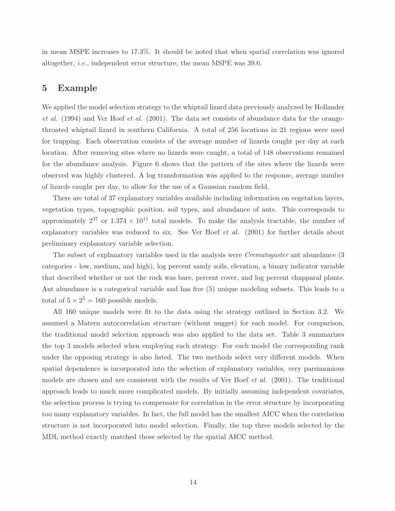
in mean MSPE increases to 17.3%. It should be noted that when spatial correlation was ignored

altogether, i.e., independent error structure, the mean MSPE was 39.6.

5 Example

We applied the model selection strategy to the whiptail lizard data previously analyzed by Hollander

et al. (1994) and Ver Hoef et al. (2001). The data set consists of abundance data for the orange-

throated whiptail lizard in southern California. A total of 256 locations in 21 regions were used

for trapping. Each observation consists of the average number of lizards caught per day at each

location. After removing sites where no lizards were caught, a total of 148 observations remained

for the abundance analysis. Figure 6 shows that the pattern of the sites where the lizards were

observed was highly clustered. A log transformation was applied to the response, average number

of lizards caught per day, to allow for the use of a Gaussian random field.

There are total of 37 explanatory variables available including information on vegetation layers,

vegetation types, topographic position, soil types, and abundance of ants. This corresponds to

approximately 237 or 1.374 × 1011 total models. To make the analysis tractable, the number of

explanatory variables was reduced to six. See Ver Hoef et al. (2001) for further details about

preliminary explanatory variable selection.

The subset of explanatory variables used in the analysis were Crematogaster ant abundance (3

categories - low, medium, and high), log percent sandy soils, elevation, a binary indicator variable

that described whether or not the rock was bare, percent cover, and log percent chapparal plants.

Ant abundance is a categorical variable and has five (5) unique modeling subsets. This leads to a

total of 5 × 25 = 160 possible models.

All 160 unique models were fit to the data using the strategy outlined in Section 3.2. We

assumed a Matern autocorrelation structure (without nugget) for each model. For comparison,

the traditional model selection approach was also applied to the data set. Table 3 summarizes

the top 3 models selected when employing each strategy. For each model the corresponding rank

under the opposing strategy is also listed. The two methods select very different models. When

spatial dependence is incorporated into the selection of explanatory variables, very parsimonious

models are chosen and are consistent with the results of Ver Hoef et al. (2001). The traditional

approach leads to much more complicated models. By initially assuming independent covariates,

the selection process is trying to compensate for correlation in the error structure by incorporating

too many explanatory variables. In fact, the full model has the smallest AICC when the correlation

structure is not incorporated into model selection. Finally, the top three models selected by the

MDL method exactly matched those selected by the spatial AICC method.

14

Table 3: Model selection results for the whiptail lizard data set. Listed are the explanatory variables

selected using AIC as the selection criterion. The rank of the model (by AIC) is provided under

both model selection strategies. Ant1 corresponds to low abundance and Ant2 corresponds to

medium abundance.

Predictors AICCSpatial

Rank

Independent

Rank

Ant1, % sand 54.1 1 66

Ant1, Ant2, % sand 54.8 2 56

Ant1, % sand, % cover 55.7 3 59

Ant1, Ant2, % sand, % cover, elevation, barerock, % chaparral 92.0 41 1

Ant1, Ant2, % sand, elevation, barerock, % chaparral 95.3 33 2

Ant1, % sand, % cover, elevation, barerock, % chaparral 95.6 38 3

6 Software

Software to perform the model selection strategy for geostatistical models described in Section

3.1 is available at www.stat.colostate.edu/∼jah and at Statlib (lib.stat.cmu.edu). The software is

compatible with both S-plus and R statistical packages, the latter which is also freely available

at Statlib. The software implements the Matern covariance function (2), but other covariance

functions can easily be adopted.

7 Conclusions

Our results demonstrate the problems that can be encountered in the selection of an appropriate set

of explanatory variables when spatial correlation is ignored. Both the AIC and MDL criteria based

on the geostatistical models performed well in the selection of appropriate explanatory variables.

Ignoring spatial correlation in the selection of explanatory variables and/or in the modeling of the

data can lead to the selection of too few explanatory variables as well as higher prediction errors. In

addition, we showed that for the sampling patterns considered here, it is advantageous to consider

a clustered type of sampling design that offers observation pairs at both small and larger distances.

We have considered the impact of ignoring spatial correlation on the selection of explanatory

variables. We must note that the concept of “all possible models” can become intractable quickly

when the number of potential explanatory variables becomes large. For this presentation, we have

assumed that only the candidate predictors enter the model as main effects with no interactions or

15

higher order terms under consideration. Thus for a data set with 10 potential explanatory variables

there are 210 = 1024 candidate models if only a single error structure is examined. But a data set

with 20 potential explanatory variables leads to 1.04×106 candidate models under the same set up.

This number will increase further if, for example, we allow interactions or higher-order polynomial

fits. Thus there are practical limitations to the proposed model selection method. To overcome

this limitation the researcher has many avenues open to her. She can perform exploratory data

analyses to reduce the number of potential explanatory variables, limit the candidate models to a

particular class (such as linear), restrict the error structure to a single form, e.g., Matern without

nugget, etc.. Often a researcher can rely on their expertise to further reduce the size of the family

of candidate models. Both spatial AICC and MDL allow the researcher to restrict the type and

class of models that best suits her needs.

Finally, other aspects of model mis-specification, such as the appropriateness of the adoption

of a Gaussian random field and stationarity autocorrelation function, are also important. Cressie

(1993) p. 289 and Smith (2000) p. 94–96 summarize some of the research on these issues.

Appendix

To give a heuristic derivation of the AIC statistic in the spatial model setup of (1), we follow

the development in Brockwell and Davis (1991), p. 303. Suppose Z = (Z1, . . . , Zn)′ and Y =

(Y1, . . . , Yn)′ are two independent realizations from model (1) at fixed locations (s1, . . . , sn) with

true parameter value ψ0 = (β0, θ0, σ20)′. Let f(·; ψ) be a candidate Gaussian density function

corresponding to the parameter vector ψ = (β, θ, σ2)′. Then by the independence of Y and Z,

Eψ

[

∆(ψ)]

= Eψ

[

Eψ

−2 log LY (ψ)|Z]

= Eψ

[

−2 log LY (ψ)]

,

where LY is the likelihood based on Y and ψ is the maximum likelihood estimate of ψ based

on Z. Using properties of the Gaussian density function and the representation σ2 = (Z −Xβ)′Ω

−1

(θ)(Z − Xβ)/n, we have

−2 log LY (ψ) = −2 log LZ(ψ) + σ−2SY (β, θ) − n, (8)

where SY (β, θ) = (Y − Xβ)′Ω−1

(θ)(Y − Xβ). The goal is find an unbiased approximation for

Eψ

[

σ−2SY (β, θ)]

of equation (8).

Using a second order Taylor series to expand SY (β, θ) in a neighborhood of (β, θ), we obtain

SY (β, θ) ≃ SY (β, θ) +(

(β, θ) − (β, θ))

′ ∂SY (β, θ)

∂(β, θ)

+1

2

(

(β, θ) − (β, θ))

′ ∂2SY (β, θ)

∂(β, θ)∂(β, θ)′

(

(β, θ) − (β, θ))

.

(9)

To evaluate the expected value of the terms in (9), we assume that standard asymptotics hold for

the MLE ψ = (β, θ, σ2)′. These are

16

i. (β, θ)′ is approximately normal with mean (β, θ)′ and asymptotic covariance matrix given by

the inverse of the Fisher information, In,

ii. for large n, I−1n can be approximated by

V (β, θ) :=

− 1

2σ2Eψ

[

∂2SY (β, θ)

∂(β, θ)∂(β, θ)′

]−1

,

iii. for large n, nσ2 = SZ(β, θ) is distributed as σ2χ2(n − p − k) and is independent of (β, θ)′,

where k is the dimension of the parameter θ associated with the correlation function for the

noise process δ(s).

Using the independence of Y and Z, we find that

EψSY (β, θ) ≃ EψSY (β, θ) +(

(β, θ) − (β, θ))

′

V (β, θ)

−1 (

(β, θ) − (β, θ))

≃ σ2n + σ2(p + k).

Hence, from the last two terms of (8), we have

Eψ(σ−2SY (β, θ)) − n = Eψ(σ−2)Eψ(SY (β, θ)) − n

≃(

σ2n − p − k − 2

n

)

−1

σ2(n + p + k) − n

= 2np + k + 1

n − p − k − 2.

The quantity

AICC = −2 log LZ(ψ) + 2np + k + 1

n − p − k − 2(10)

is an approximately unbiased estimate of the expected Kullback-Leibler information evaluated at

ψ.

The argument given above for AICC relied on the validity of standard asymptotic theory for

the maximum likelihood estimates of the parameters in the spatial model (1). In order for these

results to hold, it is likely an increasing sample size that both fills in and expands the domain under

study is required. In the statistics literature, this is often referred to as infill and increasing domain

asymptotics. Unfortunately asymptotic theory for maximum likelihood estimates for unequally

spaced data is not fully developed. In the case where data are regularly spaced on a lattice, more

complete asymptotic results can be obtained.

References

Abramowitz, M. and Stegun, I. A., editors (1965). Handbook of Mathematical Functions. Dover:

New York.

17

Akaike, H. (1973). Information theory and an extension of the maximum likelihood principle. In

Petrox, B. and Caski, F., editors, Second International Symposium on Information Theory, page

267.

Brockwell, P. J. and Davis, R. A. (1991). Time Series: Theory and Methods. Springer-Verlag.

Burnham, K. P. and Anderson, D. R. (1998). Model Selection and Inference A Practical Information

Theoretic Approach. Springer: New York.

Burnham, K. P. and Anderson, D. R. (2002). Model Selection and Inference A Practical Information

Theoretic Approach. Springer: New York, 2nd edition.

Cressie, N. A. C. (1993). Statistics for Spatial Data, revised edition. Wiley: New York.

Haining, R. (1990). Spatial data analysis in the social and enviromental sciences. Cambridge

University Press: Cambridge.

Handcock, M. S. and Stein, M. L. (1993). A Bayesian analysis of kriging. Technometrics, 35:403–

410.

Hoeting, J. A., Madigan, D., Raftery, A. E., and Volinsky, C. T. (1999). Bayesian model averaging:

A tutorial with discussion. Statistical Science, 14:382–417.

Hollander, A. D., Davis, F. W., and Stoms, D. M. (1994). Hierarchical representations of species

distributions using maps, images and signting data. In Miller, R. I., editor, Mapping the diversity

of Nature. Chapman and Hall: London.

Hurvich, C. M. and Tsai, C.-L. (1989). Regression and time series model selection in small samples.

Biometrika, 76:297–307.

Kass, R. E. and Raftery, A. E. (1995). Bayes factors. Journal of the American Statististical

Association, 90:773–795.

McQuarrie, A. D. and Tsai, C.-L. (1998). Regression and Time Series Model Selection. World

Scientific: New Jersey.

Patterson, H. D. and Thompson, R. (1971). Recovery of inter-block information when block sizes

are unequal. Biometrika, 58:545–554.

Smith, R. L. (2000). Spatial statistics in environmental science. In Nonlinear and Nonstationary

Signal Processing. Cambridge University Press.

Stein, M. L. (1999). Interpolation of Spatial Data. Springer: New York.

Sugiura, N. (1978). Further analysis of the data by Akaike’s information criterion and the finite

corrections. Communications in Statistics, Part A – Theory and Methods, 7:13–26.

Thompson, S. E. (2001). Bayesian Model Averaging and Spatial Prediction. PhD thesis, Colorado

State University.

Venables, W. N. and Ripley, B. D. (1999). Statistics and Computing. Springer: New York, third

edition.

Ver Hoef, J. M., Cressie, N., Fisher, R. N., and Case, T. J. (2001). Uncertainty and spatial linear

models for ecological data. In Hunsaker, C., Goodchild, M., Friedl, M., and Case, T., editors,

Spatial Uncertainty for Ecology: Implications for Remote Sensing and GIS Applications, pages

214–237. Springer-Verlag, New York, NY.

18

0 1 2 3 4

0.0

0.2

0.4

0.6

0.8

1.0

Distance

Cor

rela

tion

Exponentialθ2=0.75

θ2=2.00

θ2=4.00

Gaussian

Figure 1: Matern autocorrelation function for several parameter values. The horizontal axis is

the distance between points and the vertical axis is the correlation between two points at a given

distance. We used a fixed range parameter, θ1 = 2.00, with various smoothness parameter values,

θ2. Note that the exponential autocorrelation is equivalent to the Matern autocorrelation function

with θ2 = 0.50 and that the Gaussian autocorrelation function corresponds to the limiting case

such that θ2 → ∞.

0 2 4 6 8 10

0.0

0.2

0.4

0.6

0.8

1.0

Distance

Cor

rela

tion

θ1=2.00

θ1=4.00

θ1=6.00

θ1=8.00

Figure 2: Matern autocorrelation function for smoothness parameter θ2 = 1.00 and various range

parameter values, θ1.

19

220

260

300

340

AIC

C

1 1 1 1 1 1 1 1 1 1 1 1 1 1 1 1 2 2 2 2 2 2 2 2 4 4 N 3 5 3 3 32 2 2 2 2 2 2 2 3 3 4 5 3 3 4 4 3 5 3 4 3 3 5 U 4 4 53 3 3 3 5 4 4 4 5 4 5 4 5 5 4 L 5 5 4 4 5 5 5 L 5

Spatial Model Selection

350

450

550

AIC

C

N 1 2 3 4 5 1 1 1 1 2 2 2 3 3 4 1 1 1 1 1 1 2 2 2 3 1 1 1 1 2 1U 2 3 4 5 3 4 5 4 5 5 2 2 2 3 3 4 3 3 4 4 2 2 2 3 3 2L 3 4 5 4 5 5 4 5 5 5 3 3 4 4 4 3L 4 5 5 5 5 4 5

Independent Model Selection

Figure 3: AICC values for the spatial AICC and independent AICC selection strategies. Note that

the models for the spatial AICC method have been ordered from smallest to largest average AICC

over all 500 simulations. The horizontal axis lists the variables included in each model where null

refers to the intercept-only model.

20

•

•

•

•

•

•

•

•

•

•

••

•

•

•

•

•

•

••

••

••

•

•

•

•

•

•

•

•

•

••

•

•

•

•

• •

••

•

•

•

•

•

•

•••

•

•

•

•

•

•

•

•

•

•

•

•

•

••

•

•

•

•

•

•

•

•

•

••

•

•

•

•••

•

•

•

•••

••

•

•

•

••

•

•

•

x

y

0 2 4 6 8 10

02

46

810

Highly Clustered

•

•

•

•

•

•

•

•

•

•

••

•

•

•

••

• •

•• •

•

••

••

•

•

• •

•

•

•

•

•

•

•

•

•

•

•

•

•

•

•

••

•

•

•

•

•

•

•

•

•

••

•

•

••

•

•

•

•

•

•

•

•

•

•

•

••

•

••

•

••

•

•

••

•

•

•

•

•

•

•

•

•

•••

•

•

x

y

0 2 4 6 8 10

02

46

810

Lightly Clustered

•

•

••

•

•

•

•

•

•

•

•

•

•

•

•

•

•

••

•

•

•

•

•

••

•

•

•

•••

•

•

•

•

•

•

•

•

•

•

•

•

••

•

•

•

••

•

•

•

•

•

•

••

•

•

•

•

•

•

•

•

•

•

•

•

•

•

•

•

•

••

•

•

•

•

•

• •

•

•

•

•

•

•

•

•

••

•

•

•

•

x

y

0 2 4 6 8 10

02

46

810

Random Pattern

•

•

•

••

•

•

••

•

•

•

•

•

•

•

••

•

•

••

•

•

•

•

•

•

•

•

•

••

•

•

•

•

••

•

•

•

•

•

••

•

•

•

•

•

•

•

•

•

•

•

••

•

•

•

•

•

•

•

•

•

•

•

•

•

•

•

•

•

• •

•

•

•

•

••

•

••

••

•

•

•

•

•

•• •

•

•

•

x

y

0 2 4 6 8 10

02

46

810

Regular Pattern

•

•

•

•

•

•

•

•

•

•

•

•

•

•

•

•

•

•

•

•

•

•

•

•

•

•

•

•

•

•

•

•

•

•

•

•

•

•

•

•

•

•

•

•

•

•

•

•

•

•

•

•

•

•

•

•

•

•

•

•

•

•

•

•

•

•

•

•

•

•

•

•

•

•

•

•

•

•

•

•

•

•

•

•

•

•

•

•

•

•

•

•

•

•

•

•

•

•

•

•

x

y

0 2 4 6 8 10

02

46

810

Grid Design

Figure 4: Five Sampling Patterns

21

05

1015

20

Spatial AICC Independent AICC

MS

PE

Figure 5: Mean Squared Prediction Error (MSPE) for the two model selection methods based on

500 simulations.

•••••• •••••••

•• •••••

•

••••••••••

••••••••••

•••••••••• •••••

•

•••••••••••

• •••••••• ••••••••

••••••••

••••••••••••••••••••••••

•••••••••••••••••••

Longitude (degrees)

Latit

ude

(deg

rees

)

−117.6 −117.4 −117.2 −117.0 −116.8

32.6

32.8

33.0

33.2

33.4

33.6

33.8

34.0

Figure 6: Locations in southern California where the whiptail lizard was observed (n = 148).

22