model selection strategies for identifying most relevant - mediatum

Model selection strategies for identifying most

relevant covariates in homoscedastic linear models

Aleksey Min1,a, Hajo Holzmannb and Claudia Czadoa

aZentrum MathematikTechnische Universitat Munchen

Boltzmannstr. 3D-85747 Garching, Germany

and

bInstitut fur StochastikUniversitat Karlsruhe

Kaiserstraße 89D-76133 Karlsruhe, Germany

Key words and phrases: Asymptotic normality; linear regression; model selection; modelvalidation; nested models; restricted least squares.

MSC 2000: Primary 62J05; secondary 62J20.

Abstract: We propose a new method in two variations for the identification of most

relevant covariates in linear models with homoscedastic errors. In contrast to AIC, BIC and

other information criteria, our method is based on an interpretable scaled quantity. This

quantity measures a maximal relative error one makes by selecting covariates from a given

set of all available covariates. The proposed model selection procedures rely on asymptotic

normality of test statistics, and therefore normality of the errors in the regression model

is not required. In a simulation study the performance of the suggested methods along

with the performance of the standard model selection criteria AIC and BIC is examined.

The simulation study illustrates the evident superiority of the proposed method over the

AIC and the BIC, and especially when regression effects possess influence of several orders

1corresponding author, Zentrum Mathematik, Technische Universitat Munchen, Boltzmannstr. 3,D-85747 Garching , Germany, Tel.: +49/89/28917015, Fax: +49/89/28917435E-mail address: [email protected]

1

in magnitude. The accuracy of the normal approximation to the test statistics is also

investigated. The normal approximation is already satisfactory for sample sizes 50 and

100. As an illustration we analyze US college spending data from 1994.

1 Introduction

The choice of the relevant covariates in a linear regression model is an important and much

studied problem. For this purpose, various methods have been suggested in the literature.

One approach is via model selection criteria. Here one seeks to find the sub-model which

minimizes a certain information criterion, for example Akaike’s information criterion AIC

(Akaike 1974) or the Bayesian information criterion BIC (Schwarz 1978). Typically, one of

the various stepwise methods for subset selection in regression (c.f. Miller 2002) is applied

in order to find the sub-model which actually minimizes the information criterion in use.

There is a wide variety of model selection criteria in the literature, apart from AIC and

BIC we mention Mallows’ (1973) Cp, the deviance information criterion DIC as discussed

in Spiegelhalter et al. (2002) or the focused information criterion FIC of Claeskens &

Hjort (2003). For further information see the monograph of Burnham & Anderson (2002).

Another popular approach to model selection is by sequentially testing the relevant linear

restrictions determining the sub-models. For relationship between model testing using the

F−test and certain information criteria see Terasvirta & Mellin (1986).

In this paper we introduce a new type of test which is designed to validate a linear sub-

model consisting of variables with strong effects on the response, and discuss its use for

variable selection purposes. More specifically, consider the homoscedastic linear regression

model

Y = Xβ + ǫ = X1β1 + X2β2 + ǫ, (1)

2

where Y ∈ Rn is the response vector, X := [X1, X2] ∈ R

n×(p+q) is the known design

matrix and β := (β′1,β

′2)

′ ∈ Rp+q denotes the unknown regression parameter vector of

interest. For the moment the errors ǫ1, . . . , ǫn constituting ǫ in model (1) are assumed

to be independent, identically normally distributed with E(ǫ1) = 0 and V ar(ǫ1) = σ2.

However the distribution of the errors should not be necessarily a normal distribution and

later we specify it more generally depending on aims we pursue. Suppose that we want to

check the validity of the sub-model

Y = X1β1 + ǫ, (2)

where X1 ∈ Rn×p and β1 ∈ R

p. Classically one verifies model (2) by testing the point

hypothesis

H0 : β2 = 0

using the F−test. However, for many purposes it is not adequate to base a decision for or

against the sub-model (2) on testing the hypothesis H0, and some alternative methods have

been developed. Toro-Vizcarrondo & Wallace (1968), see also Wallace (1972), observed

that the sub-model may be superior to the complete model in terms of mean square error

(MSE) even if the sub-model is incorrect. Therefore they suggested to test in which model

the least squares estimator has smaller MSE. More precisely, let β = (X ′X)−1X ′Y and

βr = (X ′1X1)

−1X ′1Y denote the least squares (LS) estimator in the full model (1) and in

the sub-model (2), respectively. Here βr is also considered as a (p+ q)−dimensional vector

by filling the last q entries by 0, i.e. βr = [Y′X1(X′1X1)

−1,0′]′. For an arbitrary estimator

b of β we let MSE(b) := E [(b − β)(b − β)′], and MSE(βr) ≤ MSE(β) means that

MSE(β) − MSE(βr) is positive semidefinite. Now they suggest to test the hypothesis

HMSE : MSE(βr) ≤ MSE(β) versus KMSE : Not HMSE

3

Setting

λ := ndn(β2)

σ2, dn(β2) :=

1

nβ′

2X′2QX1

X2β2, (3)

where PX1:= X1(X

′1X1)

−1X ′1 is the projection matrix unto the column space spanned

by X1, QX1:= In − PX1

and In is the identity matrix of dimension n, Toro-Vizcarrondo

& Wallace (1968) showed that HMSE is equivalent to λ ≤ 1. Using the fact that under

the assumption of normal errors, the F-statistic corresponding to HMSE is non-central F-

distributed (in the notation of Kotz & Johnsson 1970) with non-centrality parameter λ,

Toro–Vizcarrondo & Wallace (1968) constructed a uniformly most powerful test for HMSE

versus KMSE based on the F-statistic. Hypotheses related to HMSE were investigated by

Wallace (1972) and by Yancey et al. (1973).

The hypothesis HMSE still has some drawbacks. Instead of comparing models, it com-

pares the performance of certain estimators. This is a somewhat arbitrary choice since

there are other estimators (e.g. the ridge estimator, cf. Farbrother 1975), which have

smaller MSE than the LS estimator. Further, the hypothesis HMSE compares the perfor-

mance of pre-model selection estimators, while it should compare the performance of post

model-selection estimators (cf. Leeb & Potscher 2003).

Moreover, even if the hypothesis HMSE (or H0) cannot be rejected with a large p-value,

this does not imply that the hypothesis HMSE (or H0) is actually true, and therefore no

evidence for sub-model (2) is provided. Hence, we suggest to test a hypothesis which focuses

on validating the sub-model (2). A related approach to validating parametric functional

forms of regression models (against nonparametric alternatives) was suggested by Dette

& Munk (1998). For an extensive discussion on the methodological aspects of performing

tests for model validation see Dette & Munk (2003).

In some variable selection problems one is interested not solely in identifying variables

which have a nonzero regression coefficients but in identifying variables which have a strong

4

effect on the response compared to the joint effect of the variables not selected. Therefore

we need a distance measure between the restricted model (2) and the full model (1).

Note that dn(β2) given in (3) is the squared normalized length (with factor n−1) of the

n−vector X2β2, when projected onto the orthogonal complement of the space spanned by

the columns of X1 with projection matrix QX1. Thus it provides a natural measure of

distance between the restricted model (2) and the full model (1). We propose to validate

sub-model (2) by testing the hypothesis that

H∆,n : dn(β2) > ∆ against K∆,n : dn(β2) ≤ ∆, (4)

for some ∆ > 0. Thus, rejecting H∆,n actually is a decision in favor of sub-model (2), up

to the prespecified precision ∆ and significance level α. The test of H∆,n versus K∆,n will

be based on asymptotic normality of an appropriate test statistic and therefore it does not

require normality of the homoskedastic errors in the regression model specified in (1).

Section 2 deals with testing hypotheses related to H∆,n. In Section 2.1 we introduce an

asymptotic version H∆ of H∆,n, a test statistic for H∆ and derive its asymptotic distribu-

tion. Section 2.2 is concerned with a nested testing situation, where we test a hypothesis

H∆, related to H∆, for model (2) against model (1) in the presence of another larger super-

model containing model (1) as its sub-model. The results have their main application for

deriving model selection method for identifying strong regression effects. In Section 3 we

define quantities Dα,n and Dα,n, which can be interpreted as estimated maximal relative

errors (with level α) that one makes when using the smaller sub-model. These are very

convenient for model-selection purposes, and in Section 3 we discuss how they can be

employed in a backward selection procedure.

Model selection criteria are classically divided into consistent and conservative criteria.

In certain situations such as nested models containing the true model, consistent criteria

like the BIC, choose the correct model, i.e. the minimal model that contains all covariates

5

with βi 6= 0, with a probability converging to 1. In these cases conservative criteria, like

the AIC or Mallows’ Cp, asymptotically choose models that are too large with a positive

probability, but not models that are too small. Of course, criteria such as AIC have other

advantages, e.g. when the linear model is misspecified, see Burnham & Anderson (2002).

In finite samples and in cases where there are many covariates with small but nonzero

influence, both conservative and consistent criteria will typically include some but not all

of these covariates in a somewhat arbitrary way. In contrast, model selection based on

a threshold value of Dα,n or Dα,n allows to discard covariates with a small influence in a

controlled and interpretable way, namely as long as the relative error that arises remains

below the chosen threshold t. Thus, model selection based on Dα,n or Dα,n does not aim

at finding all the covariates with nonzero influence. Rather, its goal is to find the relevant

covariates in terms of maximal relative error.

The actual performance of Dα,n and Dα,n for model selection purposes, as compared

to the AIC and the BIC are investigated in Section 4 in an extensive simulation study.

Here we also give illustrative examples for selection methods based on Dα,n and Dα,n,

respectively and investigate the quality of the normal approximation of the test statistics

introduced in Section 2. Further in Section 5, we illustrate the practical usefulness of our

method by analyzing US college spending data from 1994. Finally, Section 6 closes the

paper with conclusions and a discussion on future research. Technical assumptions and

proofs are deferred to an appendix.

6

2 Asymptotic tests for identifying large regression ef-

fects

As an illustration, suppose for the moment that the errors are normally distributed, and

let SSE(b) denote the error sum of squares of an estimator b of β. Then the statistic

T =SSE(βr) − SSE(β)

qσ2, where σ2 =

1

n − (p + q)

(

Y − Xβ)′ (

Y − Xβ)

,

is F -distributed with degrees of freedom q and (n−(p+q)) and non-centrality parameter λ,

given in (3). Since H0 is equivalent to λ = 0 and HMSE to λ ≤ 1, it is then straightforward

to construct tests for H0 and HMSE based on the F -distribution of T .

However, H∆,n is equivalent to Hλ,n : λ > n∆/σ2. Since σ2 is unknown we cannot

construct even under normality an exact test of H∆,n. However we can construct an

asymptotic test for a limiting test hypothesis of H∆,n, which does not require normal

errors in the regression model (1). In Section 2.1, we consider this limiting version of the

hypotheses H∆,n, and construct an asymptotic test for this hypothesis in case the larger

model is correct. Section 2.2 gives a corresponding test in case model (1) to which to (2)

is compared is also incorrect, assuming that there is some larger valid super-model. In

this situation, and in case of normally distributed errors, a test for HMSE is discussed in

Terasvirta & Mellin (1986).

2.1 Testing when the larger model is correct

In this section we consider testing model (2) against the larger model (1) assuming that the

larger model (1) is correct and the errors are not necessarily normally distributed. First

we introduce an asymptotic version of H∆,n. To do so, we consider the following condition

under which dn(β2) converges as n → ∞, say to d(β2).

7

Assumption 1. The regressors X are non-random and we have X ′X/n → G as n → ∞,

where G ∈ R(p+q)×(p+q) is a symmetric positive definite matrix.

Split G into blocks as follows

G =

G11 G12

G21 G22

, G11 ∈ R

p×p, G22 ∈ Rq×q, G12 = G′

21 ∈ Rp×q.

Note that dn(β2) can be rewritten as

dn(β2) =1

nβ′

2X′2(In − X1(X

′1X1)

−1X ′1)X2β2

= β′2

[

X ′2X2

n− X ′

2X1

n

(

X ′1X1

n

)−1X ′

1X2

n

]

β2

and from Assumption 1 it follows that

dn(β2) → d(β2) := β′2(G22 − G21G

−111 G12)β2 as n → ∞. (5)

Under Assumption 1, G is positive definite, which implies that G22 − G21G−111 G12 is also

positive definite. Therefore we consider the following asymptotic version of test problem

(4) given by

H∆ : d(β2) > ∆ against K∆ : d(β2) ≤ ∆. (6)

The test statistic Rn for (6) is now derived in the standard manner. To do this, we

substitute the unknown β2 in d(β2) by its consistent LS estimate β2 from model (1), i.e.

Rn := dn(β2).

It is not difficult to see that the test statistic Rn is also the normalized numerator of the

F-statistic for H0 : β2 = 0, i.e.

Rn =1

n

(

MSE(βr) − MSE(β))

=1

nY′(PX − PX1

)

Y,

with PX := X(X ′X)−1X ′. In Theorem 1 we show that Rn is an asymptotic unbiased

estimator of d (β2) and derive the asymptotic distribution of Rn when β2 6= 0.

8

Theorem 1.

i) Suppose that in model (1) with independent zero mean homoscedastic errors Assump-

tion 1 is satisfied. Then E(Rn) → d(β2) as n → ∞.

ii) Suppose that in model (1) with independent zero mean homoscedastic errors Assump-

tions 3, 4 and 5 (cf. the appendix) are satisfied. If d(β2) > 0 we have that√

n(

Rn −

d(β2)) L−→ N

(

0, 4σ2d(β2))

as n → ∞.

The proof of Theorem 1 is given in the appendix. Using Theorem 1, we construct an

asymptotic test for H∆ : d(β2) > ∆ versus K∆ : d(β2) ≤ ∆ as follows. Given ∆ > 0,

reject H∆ with level α > 0 if

Rn ≤ ∆ + 2σuα

√∆/

√n, (7)

where uα denotes the α-quantile of the standard normal distribution.

2.2 Testing when having a valid super-model

Theorem 1 is only valid if the larger model (1) is correct. However, if we apply the test

sequentially, then we will possibly also have the situation where the larger model is not

true either, because we already excluded covariates with too small an influence, which are

however non-zero. Therefore, we now study the situation where the larger model is also not

correct. However, we assume that at least the linear regression model with all covariates

is correct, thus, there is a valid super-model.

Changing the notation slightly, suppose that we already erroneously believe that at

most the following sub-model

Y = X1β1 + X2β2 + ǫ, (8)

9

of the true super-model

Y = Zβ + ǫ, Z = [X1, X2, X3], β = [β′1,β

′2,β

′3]

′, (9)

contains all the relevant covariates, and that we want to check the validity of the smaller

sub-model Y = X1β1+ǫ. to Note that X1 ∈ Rn×p, X2 ∈ R

n×q1 , X3 ∈ Rn×q2 , β1 ∈ R

p, β2 ∈

Rq1 , β3 ∈ R

q2 . Further the errors ǫi’s are independent identically distributed (i.i.d.) with

E(ǫ1 = 0), V ar(ǫ1) = σ2 and not necessarily normal. For convenience let X := [X1, X2]

and let QX,X1:= PX − PX1

. Now define

dn(β2,β3) :=1

n

(

β′2X

′2 + β′

3X′3

)

QX,X1

(

X2β2 + X3β3

)

. (10)

The quantity dn(β2,β3) is the normalized (by a factor of 1/n) length of the n−vector

X2β2 + X3β3 when orthogonally projected by QX,X1onto the orthogonal complement of

the space spanned by the column vectors of X1 in the space spanned by those of X. As in

Section 2.1 we impose here the following assumption on the design matrix Z.

Assumption 2. The regressors Z are non-random and we have Z ′Z/n → G as n → ∞,

where G ∈ R(p+q1+q2)×(p+q1+q2) is a symmetric positive definite matrix.

Split G into blocks as follows

G =

G11 G12 G13

G21 G22 G23

G31 G32 G33

,

where G11 ∈ Rp×p, G22 ∈ R

q1×q1 , G33 ∈ Rq2×q2 , G12 = G′

21 ∈ Rp×q1 , G13 = G′

31 ∈ Rp×q2 and

G23 = G′32 ∈ R

q1×q2 . Under Assumption 2 it follows also for n → ∞ that

X ′X/n →

G11 G12

G21 G22

=: Gr1,2

.

10

Lemma 1. Let Assumption (2) hold for the design matrix Z of model (9). Then

dn(β2,β3) → d(β2,β3) := β′2Aβ2 + β′

3BA−1B′β3 + 2β′3Bβ2 as n → ∞,

where

A := G22 − G21G−111 G12, B := G32 − G31G

−111 G12. (11)

The proof of Lemma 1 is given in the appendix.

For ∆ > 0 Lemma 1 allows to consider a testing problem

H∆ : d(β2,β3) ≥ ∆ against K∆ : d(β2,β3) < ∆, (12)

which is an asymptotic version of

H∆,n : dn(β2,β3) ≥ ∆ against K∆,n : d(β2,β3) < ∆.

The test statistic Rn for (12) is derived by substituting β2 and β3 in d(β2,β3) with their

consistent LS estimates β2 and β3 based on model (9). Thus

Rn := dn(β2, β3).

It should be noted that the test statistic Rn can be rewritten as

Rn =1

n

(

MSE(βr1) − MSE(βr1,2

))

=1

nY′(PX − PX1

)

Y,

where βr1is the restricted LS estimator in model (2) and βr1,2

the restricted LS estimator

in model (8). Here additional zeros have been added to obtain the same dimension as β.

In the appendix we sketch the proof of the following result:

Theorem 2.

i) Suppose that in model (9), Assumption 2 is satisfied. Then E(Rn) → d(β2,β3) as

n → ∞.

11

ii) Suppose that in model (9), Assumptions 3, 6 and 7 (cf. the appendix) are satisfied. If

d(β2,β3) > 0 we have that√

n(

Rn − d(β2,β3)) L−→ N

(

0, 4σ2d(β2,β3))

as n → ∞.

Theorem 2 allows to construct an asymptotic test for the testing problem (12). Indeed,

given ∆ > 0, reject H∆ versus K∆ with level α > 0 if

Rn ≤ ∆ + 2σuα

√∆/

√n, (13)

where σ is an estimate of σ based on the full super-model (9).

3 Model validation and model selection

Test decisions based on (7) or (13) will obviously strongly depend on the choice of ∆.

For example, in (7), ∆ is a threshold for d(β2), the limit of the distance dn(β2), which

as mentioned above measures the normalized (with factor n−1) squared distance of the

projected vector X2β2. This has to be seen in relation with the total normalized squared

length β′X ′Xβ/n, and thus, a general recommendation for a numerical value of ∆ (like

0.1) does not make sense. Therefore, in the following we suggest objective procedures for

choosing ∆, and discuss how the resulting tests can be used for model selection purposes

within a backward selection procedure.

3.1 Model selection based on Dα,n

First consider the hypothesis H∆ in (6) for arbitrary ∆. Using (7) one can, for a given

level α (e.g. α = 0.05), determine a critical threshold ∆crit(α, n) for which H∆crit(α,n) can

be rejected at level α, while H∆ cannot be rejected for ∆ < ∆crit(α, n), i.e. ∆crit(α, n) is

defined as

∆crit(α, n) :=(

(

Rn + σ2u2α/n)1/2 − σuα/

√n)2

.

12

Then we suggest to normalize ∆crit(α, n) by an estimate of the total normalized squared

length and take square roots to obtain

Dα,n :=( ∆crit(α, n)

β′X ′Xβ/n

)1/2

,

where β is the LSE of β in (1). The quantity Dα,n can be nicely interpreted as the estimated

maximal relative error one makes (with level α) if one uses sub-model (2) instead of the

full model (1). In fact, one has Dα,n → [d(β2)/(β′Gβ)]

1/2:= D in probability as n → ∞.

Note that D depends on the unknown regression vector β which for brevity is suppressed

in the following. Variable identification with strong effects on the response now proceeds

in terms of Dα,n: If Dα,n is less than some fixed value which we allow as maximal relative

error (say 0.1), we identify the variables included in the smallest sub-model as variables

with strong effects.

Let us describe how the above method can be used in a backward selection procedure.

After fixing the level α, we compute Dα,n for all sub-models of the full model (1) which

exclude one covariate. Let the sub-model with minimal Dα,n, denoted by D1α,n, be M1.

Next we compute Dα,n, relative to the full model (1), for all sub-models of M1 which

exclude a further covariate. Let the sub-model among the sub-models of M1 with minimal

Dα,n, denoted by D2α,n, be M2. Let us stress that in each step we compute Dα,n relative to

the full model (which we assume to be correct so that we have no misspecification), since

we possibly already excluded covariates with small but still notable influence. In this way

we obtain a decreasing sequence of sub-models M1 ⊃ M2 ⊃ . . . with increasing sequence

D1α,n ≤ D2

α,n ≤ . . . with corresponding relative errors w.r.t. the full model (1). One can

now choose the model from the sequence Mi, e.g. as the model for which the relative

error is just below some threshold t (e.g. 0.1). Note that we use Dα,n, which is always

normalized by the same factor βX ′Xβ/n. Therefore, the order M1 ⊃ M2 ⊃ . . . in which

the model is reduced is the same as for the F-test and the AIC and BIC, only the stopping

13

is more transparent as it is based on the maximal relative error. We further discuss this

in the simulation study in Section 4.

3.2 Model selection based on Dα,n

For the testing problem H∆ versus K∆ in (12) and for a given level α, the threshold

∆crit(α, n) for which H∆crit(α,n) can be rejected at level α, while H∆ cannot be rejected for

∆ < ∆crit(α, n), is determined by using (13) as follows:

∆crit(α, n) :=(

(

Rn + σ2u2α/n)1/2 − σuα/

√n)2

,

where σ is an estimator of σ in (9). We suggest to normalize ∆crit(α, n) by an estimate of

the total normalized length in model (8)

Dα,n :=( ∆crit,α,n

β′r1,2

X ′Xβr1,2/n

)1/2

,

where βr1,2is the LSE in (8). The interpretation of Dα,n is also that of an estimated

relative error, since d(β2,β3) only involves the normalized length of Zβ when orthogonally

projected onto the orthogonal complement of the column space of X1 in that of X =

[X1, X2]. However, it takes into account the whole contribution of X2β2 + X3β3, and

is therefore not exclusively relative to the intermediate model (8). Note that Dα,n →√

d(β2,β3)/β′r1,2

Gr1,2βr1,2

=: D in probability as n → ∞. Note that D depends on β2 and

β3, which we omit in the sequel.

The backward selection procedure based on Dα,n proceeds as follows. After fixing the

level α and a threshold value t for Dα,n, we compute Dα,n for all sub-models of the correct

super-model M0 which exclude one covariate. Let the sub-model of M0 with minimal Dα,n,

denoted by D1α,n, be M1. Next we compute Dα,n, relative to M1, for all sub-models of M1

which exclude a further covariate. Thus here we are possibly already in the situation where

14

the intermediate model is incorrect, since we compare relative to the (possibly already

incorrect) sub-model M1. Let the sub-model among the sub-models of M1 with minimal

Dα,n, denoted by D2α,n, be M2. In this way we obtain a decreasing sequence of sub-models

M1 ⊃ M2 ⊃ . . . with (not necessarily increasing) relative errors D1α,n, D2

α,n, . . .. Now one

chooses the first model from the sequence Mi for which Diα,n is below the threshold t, while

Di+1α,n is larger than the threshold t. Note that the denominator of Di

α,n changes in each

step, since the intermediate models (8) are changing. This implies that the order in which

the models are reduced M1 ⊃ M2 ⊃ . . . may be different from that for the AIC, the BIC

and the method based on Dα,n.

4 Simulation study

In the simulation study we consider three different scenarios for the regression effects. First

we choose strong equal regression effects (Scenario 1), one set of variables with very strong

and one set with medium strength regression effects (Scenario 2) and finally regression

effects which vary from very strong to weak effects (Scenario 3). The specific values of the

regression coefficients are given in Table 1 where β0 is an intercept. For i = 1, . . . , 6

Table 1: Simulation setups

Scenarios for β = (β0, β1, β2, β3, β4, β6)′ Sample size n

1 β = (2, 2, 2, 2, 0.1, 0.1, 0.1)′ a) 200

2 β = (10, 5, 5, 1, 1, 0.05, 0.05)′ b) 400

3 β = (10, 15, 7, 3, 1.5, 0.7, 0.3)′ c) 1000

d) 5000

Error distribution

i) t-distribution with 5 degrees of freedom

ii) standard normal distribution

the covariate vector xi is drawn independently from a uniform distribution on [−1, 1]n.

The n−dimensional unit vector x0 corresponds to the intercept β0. For the corresponding

15

design matrix X = [x0,x1,x2,x3,x4,x5,x6] Assumption 1 (Assumption 2) is satisfied with

X ′X/n → G = diag (1, 1/3, . . . , 1/3) (Z ′Z/n → G = diag (1, 1/3, . . . , 1/3)) .

As error distribution we choose a t−distribution with 5 degrees of freedom (df) and the

standard normal distribution. Note that the errors ǫi for i = 1, . . . , n should be scaled by

a factor SF in such a way that observations with signal to noise ratio (SNR) larger than

2 approximately form 40%–50% of the whole data. Here SNR is just a ratio of mean to

standard deviation of an observation. Finally sample sizes n = 200, 400, 1000 and 5000 are

investigated. Thus for each combination of β, n and an error distribution given in Table 1

we apply our methods.

In Section 4.1 we illustrate in detail how our methods work in Scenario 1 and 2 for

regression coefficients. Section 4.2 contains a simulation study in which we investigate the

performance of model selection based on Dα,n and Dα,n as compared to the standard model

selection criteria AIC and BIC. We give results for two choices of the threshold t and discuss

its choice. Finally in Section 4.3 we investigate the quality of the normal approximation in

Theorems 1 and 2 for t−distributed errors. In all model selection methods, we use backward

elimination and always keep the intercept, thus only choosing from the covariates.

4.1 Illustrating examples

Consider Scenario 1 where the vector of regression coefficients β is set as β = (2, 2, 2, 2, 0.1,

0.1, 0.1)′. Now we chose n = 200 and t−distributed errors with 5 df scaled by the factor

SF =√

0.8. This results that the variance of scaled errors is equal to 1.33. Table 2 contains

the results of our model selection procedures for one sample, together with the estimated

Dα,n and Dα,n as wells as with the true values D and D. Models which contain x1,x2 and

x3 result in estimated relative error (Dα,n or Dα,n) around 0.1, however models which miss

16

one of x1,x2 and x3 have estimated relative error larger than 0.4. Thus, there are only

two reasonable choices for possible models. Either one is willing to except a relative error

at about 0.2 and only keeps x1,x2,x3, or one keeps all the covariates.

Table 2: Results of model selection procedure based on the Dα,n− and Dα,n−methods for

a data set of size n = 200 simulated with β = (2, 2, 2, 2, 0.1, 0.1, 0.1)′ and t−distributed

errors with 5 df scaled by SF =√

0.8. The level α is equal to 0.05.

step i sub-model discarded cov. Diα,n D Di

α,n D

1 x0,x1,x2,x3,x4,x5 x6 0.106 0.020 0.106 0.020

2 x0,x1,x2,x3,x5 x4 0.107 0.028 0.107 0.020

3 x0,x1,x2,x3 x5 0.113 0.035 0.112 0.020

4 x0,x1,x3 x2 0.488 0.040 0.488 0.408

5 x0,x3 x3 0.643 0.578 0.503 0.447

For the second illustration we consider Scenario 2 for regression coefficients, t−distribu-

ted errors with 5 df and sample sizes n = 200, 400, 1000 and 5000. Note that this scenario

has several orders of magnitude for the regression coefficients β’s. The scaling factor SF is

set to 4 and it ensures for example that 48% observations have a SNR>2 for n = 200. Table

3 contains the results of the model selection procedure for one sample, together with the

Table 3: Results of model selection procedure based on the Dα,n−method for a data set

simulated with β = (10, 5, 5, 1, 1, 0.05, 0.05)′ and t−distributed errors with 5 df scaled by

SF = 4. Note α = 0.05, β1 = (10, 5, 5)′, β2 = (1, 1, 0.05, 0.05)′ and D ≈ 0.08.

Step i Sub-Model discarded Diα,n

covariate n =

200 400 1000 5000

1 x0,x1,x2,x3,x4,x6 x5 0.120 0.048

x0,x1,x2,x3,x4,x5 x6 0.076 0.022

2 x0,x1,x2,x3,x4 x5 0.080 0.030

x0,x1,x2,x3,x4 x6 0.120 0.057

3 x0,x1,x2,x4 x3 0.061

x0,x1,x2,x3 x4 0.125 0.105 0.070

4 x0,x1,x2 x3 0.147 0.127 0.094

x0,x1,x2 x4 0.081

5 x0,x2 x1 0.350 0.263

x0,x1 x2 0.293 0.272

17

values of Dα,n. Here we are interested in identifying the large effects, namely covariates

x0, x1 and x2 in the presence of moderate effects x3 and x4. Thus the regression vector

β is split as (β′1,β

′2)

′, where β1 = (10, 5, 5)′ and β2 = (1, 1, 0.05, 0.05)′. Further the true

theoretical value of D for identifying β1 is equal to 0.08. If we would now use the threshold

t = 0.1 then the important covariates x0, x1 and x2 should be chosen by the Dα,n−method.

In each column of Table 3 the value of Diα,n is bolded as soon as Di

α,n > 0.1 for a first

time. This implies that the method chooses the previous model above. For n = 200 our

model selection procedure with t = 0.1 does not choose any sub-model with 5 covariates

and therefore the full model cannot be simplified. When now sample sizes increases to

400, then the sub-model with x0,x1,x2,x3 and x4 is identified which contains the medium

regression effects x3 and x4. For n = 1000 and n = 5000 the desired sub-model is detected

with threshold t = 0.1, even though the empirical values of Dα,n are slightly larger then

the true value D = 0.8. This example shows that for small and moderate sample sizes n

such as 200 or 400 a correction for threshold value t is needed. We discuss this point in

the next section in more detail.

4.2 Model selection performance

Here we report results of an extensive simulation study to compare the performance of

our model selection criteria based on the Dα,n− and Dα,n−methods with the AIC and the

BIC. For the Dα,n− and Dα,n−methods, in each simulation we choose the level α = 0.05

and sample size 200 as wells as 400.

Table 4 displays the frequency of chosen sub-models for 1000 data sets simulated

with β = (2, 2, 2, 2, 0.1, 0.1, 0.1)′, a fixed design matrix X and the two error distributions

from Table 1. The t−errors are scaled with SF =√

0.8 while the normal errors are

scaled with SF =√

4/3. This implies that the both type of scaled errors have the same

18

variance and 44% of observations have the SNR>2 for n = 200. Obviously, this regression

model has three covariates x0, x1, x2 and x3 corresponding to β1 = (2, 2, 2, 2)′ which we

want to identify. The true value of D (D) for identifying these is equal to 0.04 (0.02).

However as we noticed in the previous section the threshold value t should be corrected

for small and moderate sample sizes. Therefore we chose 0.1 or 0.15 as the threshold t

for the Dα,n−method, which are obtained by rounding 3 · 0.04 and 4 · 0.04 to the nearest

numbers 0.1, 0.15 or 0.2. From our experience the true relative error D (D) for choosing

the threshold t for the Dα,n−method (Dα,n−method) should be multiplied by the factor 2,

3 or even 4 (3,4 or even 5) for sample sizes 200 or 400 when about 50% observations have

SNR larger than 2 and only 6 covariates are under consideration. For both methods we

Table 4: Number of times specific sub-models are chosen using Dα,n, Dα,n, BIC and AIC

among 1000 simulated data sets with β = (2, 2, 2, 2, 0.1, 0.1, 0.1)′. We want to identify

covariates x0,x1,x2, and x3. Note β1 = (2, 2, 2, 2)′, β2 = (0.1, 0.1, 0.1)′, D ≈ 0.04 for

the Dα,n−method and β1 = (2, 2, 2, 2)′, β2 = 0.1, β3 = (0.1, 0.1)′, D ≈ 0.02 for the

Dα,n−method.

t-errors with 5 degrees of freedom (SF =√

0.8)

Sub-model Dα,n Dα,n BIC AIC

t = 0.1 t = 0.15 t = 0.1 t = 0.15

n = n = n = n = n = n =

200 400 200 400 200 400 200 400 200 400 200 400

x0,x1,x2,x3,x4,x5 283 3 4 0 271 0 1 0 3 5 50 105

x0,x1,x2,x3,x5,x6 271 11 4 1 261 6 2 1 2 16 60 103

x0,x1,x2,x3,x4,x6 289 5 5 0 281 3 3 0 3 3 56 96

x0,x1,x2,x3,x4 44 118 54 1 41 59 23 0 64 92 165 155

x0,x1,x2,x3,x5 34 88 49 2 40 38 21 0 45 65 129 134

x0,x1,x2,x3,x6 46 76 42 0 49 29 15 0 50 61 132 145

x0,x1,x2,x3 33 699 842 996 57 865 935 999 833 758 408 262

Normal errors (SF =p

4/3)

x0,x1,x2,x3,x4,x5 318 5 1 0 313 1 0 0 1 7 44 100

x0,x1,x2,x3,x5,x6 277 4 3 0 272 1 1 0 3 6 55 123

x0,x1,x2,x3,x4,x6 305 4 3 0 296 1 1 0 4 4 64 84

x0,x1,x2,x3,x4 26 106 48 0 28 38 18 0 48 70 163 159

x0,x1,x2,x3,x5 31 98 48 0 33 34 22 0 47 66 150 145

x0,x1,x2,x3,x6 23 100 47 0 23 41 15 0 40 73 113 133

x0,x1,x2,x3 20 683 850 1000 35 884 943 1000 857 774 411 256

19

use the same threshold values in order to illustrate the difference between them.

For t−errors both methods choose in over 99% the sub-model with three important

covariates x1,x2 and x3 when t = 0.15 and n = 400. They clearly outperform BIC (AIC),

which rather chooses the sub-model with x1,x2 and x3 only in 76% (26%). If the sample size

decreases from 400 to 200 then the Dα,n−method is comparable with BIC and outperforms

AIC. The Dα,n− method performs here clearly better than BIC and AIC. If the threshold

t = 0.1 then our methods are comparable with BIC only for n = 400 while for n = 200

their performance is very poor with respect to BIC and AIC. It should be noted that when

a sample size increases then BIC and AIC start to detect the small and medium regression

effects. In contrast, in this situation the precision of our methods increases and they start

to choose a smaller model with all large regression effects. For normal errors we get similar

results as for the t−error case.

We performed simulations for regression coefficients from Scenario 2 and the same

design matrix X in a similar manner. The t−errors are now scaled with SF = 4 while

the normal errors are scaled with SF = 4√

5/3. This ensures that the scaled errors have

the same variance and 48% of the observations have SNR>2 for n = 200. Here we would

like to identify strong regression effects x0, x1 and x2 corresponding to β1 = (10, 5, 5)′ in

the presence of the moderate effect regressors x3 and x4. The true value of D (D) for

identifying them is equal to 0.08 (0.05). We set the threshold t for both methods to 0.15

and 0.2 which are argued by multiplying the true relative error D = 0.08 by 2 and 3 and

then rounding them to the nearest numbers 0.1, 0.15 or 0.2.

Table 5 displays how often sub-models have been selected for 1000 data sets simulated

according to the above setup. We see that the correction of the true relative error by

multiplying with 2 (t = 0.15) is not enough for n = 200. To see a better performance

of our methods in comparison with BIC and AIC, the sample size should be increased to

20


among 1000 simulated data sets with β = (10, 5, 5, 1, 1, 0.05, 0.05)′. We want to identify

covariates x0,x1 and x2. Note β1 = (10, 5, 5)′, β2 = (1, 1, 0.05, 0.05)′, D ≈ 0.08 for

the Dα,n−method and β1 = (10, 5, 5)′, β2 = 1, β3 = (1, 0.05, 0.05)′, D ≈ 0.05 for the

Dα,n−method.t-errors with 5 degrees of freedom (SF = 4)


t = 0.15 t = 0.2 t = 0.15 t = 0.2

n = n = n = n = n = n =

200 400 200 400 200 400 200 400 200 400 200 400

x0,x1,x2,x3,x4,x5 10 1 0 0 7 0 0 0 3 5 40 99

x0,x1,x2,x3,x5,x6 6 1 0 0 4 1 0 0 1 0 6 9

x0,x1,x2,x3,x4,x6 12 0 0 0 11 0 0 0 3 4 60 102

x0,x1,x2,x4,x5,x6 7 0 0 0 2 0 0 0 1 0 7 8

x0,x1,x2,x3,x4 130 3 3 0 70 0 0 0 58 179 230 435

x0,x1,x2,x3,x5 19 0 0 0 7 0 0 0 1 5 28 18

x0,x1,x2,x3,x6 26 0 1 1 10 0 0 0 6 2 32 22

x0,x1,x2,x4,x5 22 0 1 0 8 0 0 0 3 5 38 21

x0,x1,x2,x4,x6 29 0 2 0 13 0 0 0 5 3 41 11

x0,x1,x2,x5,x6 2 0 0 0 1 0 0 0 0 0 7 1

x0,x1,x2,x3 211 112 72 2 180 14 12 0 169 203 131 116

x0,x1,x2,x4 251 112 82 0 215 27 23 0 225 237 203 119

x0,x1,x2,x5 26 5 1 0 6 0 1 0 8 5 21 5

x0,x1,x2,x6 22 2 5 0 5 0 0 0 1 7 17 7

x0,x1,x2 227 764 833 997 461 958 964 1000 516 345 139 27


80/3)

x0,x1,x2,x3,x4,x5 5 0 0 0 1 0 0 0 0 3 39 94

x0,x1,x2,x3,x5,x6 5 0 0 0 1 0 0 0 0 0 8 7

x0,x1,x2,x3,x4,x6 4 0 0 0 1 0 0 0 0 1 49 95

x0,x1,x2,x4,x5,x6 3 0 0 0 1 0 0 0 0 0 8 7

x0,x1,x2,x3,x4 129 0 1 0 70 0 0 0 64 184 246 436

x0,x1,x2,x3,x5 19 0 0 0 12 0 0 0 8 4 37 21

x0,x1,x2,x3,x6 16 0 0 0 6 0 0 0 5 6 21 24

x0,x1,x2,x4,x5 25 0 0 0 10 0 0 0 5 4 37 17

x0,x1,x2,x4,x6 38 0 0 0 10 0 0 0 8 5 45 18

x0,x1,x2,x5,x6 4 0 0 0 2 0 0 0 0 1 4 3

x0,x1,x2,x3 228 92 70 1 190 12 11 0 176 187 152 101

x0,x1,x2,x4 273 98 78 0 234 10 18 0 233 217 202 130

x0,x1,x2,x5 27 4 6 0 10 0 0 0 10 3 15 5

x0,x1,x2,x6 26 5 3 0 14 0 0 0 9 13 20 6

x0,x1,x2 198 801 842 999 438 978 970 1000 482 372 117 36

400. The correction by the factor 3 shows that our methods clearly outperform BIC and

AIC for the both sample sizes. A change of the error distribution does not change the

results by much. If a larger proportion of observations has a SNR larger than 2 then a

correction factor 2 becomes acceptable. Table 6 shows the same results as in Table 5 but

21


among 1000 simulated data sets with β = (10, 5, 5, 1, 1, 0.05, 0.05)′. We want to identify

covariates x0,x1 and x2. Note β1 = (10, 5, 5)′, β2 = (1, 1, 0.05, 0.05)′, D ≈ 0.08 for

the Dα,n−method and β1 = (10, 5, 5)′, β2 = 1, β3 = (1, 0.05, 0.05)′, D ≈ 0.05 for the

Dα,n−method.t-errors with 5 degrees of freedom (SF = 2)


t = 0.15 t = 0.2 t = 0.15 t = 0.2

n = n = n = n = n = n =

200 400 200 400 200 400 200 400 200 400 200 400

x0,x1,x2,x3,x4,x5 0 0 0 0 0 0 0 0 14 25 129 160

x0,x1,x2,x3,x5,x6 0 0 0 0 0 0 0 0 0 0 0 1

x0,x1,x2,x3,x4,x6 0 0 0 0 0 0 0 0 11 10 147 148

x0,x1,x2,x4,x5,x6 0 0 0 0 0 0 0 0 0 0 3 0

x0,x1,x2,x3,x4 0 0 0 0 0 0 0 0 621 919 637 690

x0,x1,x2,x3,x5 0 0 0 0 0 0 0 0 3 0 4 0

x0,x1,x2,x3,x6 0 0 0 0 0 0 0 0 2 2 5 0

x0,x1,x2,x4,x5 0 0 0 0 0 0 0 0 2 0 8 0

x0,x1,x2,x4,x6 0 0 0 0 0 0 0 0 4 0 4 0

x0,x1,x2,x3 13 1 0 0 0 0 0 0 116 11 19 0

x0,x1,x2,x4 18 0 0 0 2 0 0 0 197 31 43 1

x0,x1,x2,x5 0 0 0 0 0 0 0 0 1 0 0 0

x0,x1,x2 969 999 1000 1000 998 1000 1000 1000 29 2 1 0


20/3)

x0,x1,x2,x3,x4,x5 0 0 0 0 0 0 0 0 19 14 139 154

x0,x1,x2,x3,x5,x6 0 0 0 0 0 0 0 0 0 0 2 0

x0,x1,x2,x3,x4,x6 0 0 0 0 0 0 0 0 11 25 124 153

x0,x1,x2,x4,x5,x6 0 0 0 0 0 0 0 0 0 0 3 0

x0,x1,x2,x3,x4 0 0 0 0 0 0 0 0 618 921 663 691

x0,x1,x2,x3,x5 0 0 0 0 0 0 0 0 3 0 7 0

x0,x1,x2,x3,x6 0 0 0 0 0 0 0 0 6 0 5 0

x0,x1,x2,x4,x5 0 0 0 0 0 0 0 0 2 0 0 0

x0,x1,x2,x4,x6 0 0 0 0 0 0 0 0 5 1 7 1

x0,x1,x2,x3 8 0 0 0 1 0 0 0 125 16 18 0

x0,x1,x2,x4 11 0 0 0 1 0 0 0 188 22 32 1

x0,x1,x2 981 1000 1000 1000 998 1000 1000 1000 23 1 0 0

with different scale factors SF ’s. The values for SF are chosen in such a way that 80%

of observations have SNR>2. We see that for the both error distributions our methods

identify the desired model with a correction factor 2 or 3 for the true threshold correctly,

thus improving the precision of the methods. In contrast BIC and AIC start to choose

strong and intermediate regression effects together. A change of the error distribution does

not change the results by much.

22

Finally consider a scenario with no clearly separated orders of magnitudes for the β’s.

We choose β = (10, 15, 7, 3, 1.5, 0.7, 0.3)′, i.e. Scenario 3 in Table 1. Thus regression effects

decrease without having strong separation of effects. The t−errors are now scaled with

SF = 4 while the normal errors are scaled with SF = 4√

5/3. The scaled errors for

both error distributions thus have the same variance and 47.5% of the observations have

SNR>2 for n = 200. Now we want to identify covariates x0, x1, x2 and x3 corresponding

to β = (β0, β1, β2, β3)′. The true value of D (D) for identifying them is equal to 0.07 (0.06).

As above, we set the threshold as t = 0.15 and t = 0.2 which are motivated by multiplying

0.07 by 2 and 3. Table 7 contains the results of the model selection procedures for 1000

data sets simulated within Scenario 3. Here we see that a correction factor 2 (t = 0.15)

works well for our both methods and they outperform BIC and AIC for sample sizes 200

and 400. Thus for n = 200 the Dα,n−method (Dα,n−method) chooses the sub-model with

x0,x1,x2,x3 in 64% (74%) while the BIC does so in 35%. If now the threshold 0.2 is used

then the Dα,n−method identifies the desired model still better than the BIC (59% versus

35%) while Dα,n−method fails to do this (25% versus 35%). This indicates that when there

are no clear strong effects then the choice of the correction factor for the desired relative

errors D and D should be done carefully.

Now we discuss our results using a false discovery rate (FDR) criterion for multiple test-

ing problems introduced by Benjamini & Hochberg (1995). This criterion has been found

especially useful when a large number of covariates are under consideration. Therefore its

use became quite popular for microarray data (see e.g. Drigalenko & Elston (1997)), where

an experimenter aims to detect a few genes relevant to a disease among many ten thousands

or even hundred thousands of genes. In order to introduce the FDR criterion the related

quantities such as the number of true positives (TP), the number of false negatives (FN),

the number of false positives (FP) should be characterized. In a model selection procedure

23


among 1000 simulated data sets with β = (10, 15, 7, 3, 1.5, 0.7, 0.3)′. We want to identify

covariates x0,x1,x2 and x3. Note β1 = (10, 15, 7, 3)′, β2 = (1.5, 0.7, 0.3)′, D ≈ 0.07 for

the Dα,n−method and β1 = (10, 15, 7, 3)′, β2 = 1.5, β3 = (0.7, 0.3)′, D ≈ 0.06 for the

Dα,n−methodt-errors with 5 degrees of freedom (SF = 4)


t = 0.15 t = 0.2 t = 0.15 t = 0.2

n = n = n = n = n = n =

200 400 200 400 200 400 200 400 200 400 200 400

x0,x1,x2,x3,x4,x5 4 0 0 0 3 0 0 0 57 156 297 496

x0,x1,x2,x3,x5,x6 0 1 0 0 0 1 0 0 1 2 23 9

x0,x1,x2,x3,x4,x6 3 0 0 0 1 0 0 0 16 26 127 146

x0,x1,x2,x3,x4 257 17 5 0 129 3 1 0 499 648 433 337

x0,x1,x2,x3,x5 37 2 1 0 8 0 0 0 50 33 41 6

x0,x1,x2,x3,x6 5 0 0 0 0 0 0 0 8 4 13 1

x0,x1,x2,x4,x5 3 0 0 0 0 0 0 0 3 0 0 0

x0,x1,x2,x3 642 929 568 157 743 693 256 13 349 131 65 5

x0,x1,x2,x4 41 14 35 2 40 4 4 0 11 0 1 0

x0,x1,x2,x5 0 0 1 0 1 0 0 0 1 0 0 0

x0,x1,x2 8 37 390 841 75 299 739 987 5 0 0 0


80/3)

x0,x1,x2,x3,x4,x5 2 0 0 0 1 0 0 0 59 172 290 531

x0,x1,x2,x3,x5,x6 1 0 0 0 0 0 0 0 4 8 18 20

x0,x1,x2,x3,x4,x6 0 0 0 0 0 0 0 0 19 22 118 123

x0,x1,x2,x3,x4 270 14 1 0 134 1 0 0 505 633 434 311

x0,x1,x2,x3,x5 34 2 0 0 8 0 0 0 49 31 43 9

x0,x1,x2,x3,x6 5 0 0 0 0 0 0 0 7 9 16 2

x0,x1,x2,x4,x5 1 0 0 0 1 0 0 0 0 0 0 0

x0,x1,x2,x4,x6 2 0 0 0 0 0 0 0 2 0 0 0

x0,x1,x2,x3 643 932 593 152 753 697 255 11 345 125 80 4

x0,x1,x2,x4 28 7 39 0 30 0 3 0 8 0 1 0

x0,x1,x2,x5 1 0 1 0 0 0 0 0 0 0 0 0

x0,x1,x2 13 45 366 848 73 302 742 989 2 0 0 0

the relevant covariates to the response can be identified or not. Now the number of TP

describes the number of correctly identified relevant covariates while the number of FN

describes the number of relevant covariates which are not identified. Their sum results in

the number p of the important covariates for the response (dimension of β1). Similarly,

non-relevant covariates can be wrongly identified as relevant or not. The number FP is just

the number of non-relevant regression effects which are wrongly identified as important.

24

Table 8: Averaged values of true positives (TP), false negatives (FN), false positives (FP)

and the corresponding false discovery rate (FDR) based on the averaged values among

1000 simulated data sets for t−errors with 5 degrees of freedom.β = (2, 2, 2, 2, 0.1, 0.1, 0.1)′, SF =

√0.8 and desired sub-model x0,x1,x2,x3

Dα,n Dα,n BIC AIC

t = 0.1 t = 0.15 t = 0.1 t = 0.15

n = n = n = n = n = n =

200 400 200 400 200 400 200 400 200 400 200 400

TP 4 4 4 4 4 4 4 4 4 4 4 4

FN 0 0 0 0 0 0 0 0 0 0 0 0

FP 1.81 0.320 0.171 0.005 1.756 0.144 0.071 0.002 0.175 0.266 0.758 1.042

FDR 0.312 0.074 0.041 0.001 0.305 0.035 0.017 0.000 0.042 0.062 0.159 0.207

β = (10, 5, 5, 1, 1, 0.05, 0.05)′, SF = 4 and desired sub-model x0,x1,x2

Dα,n Dα,n BIC AIC

t = 0.15 t = 0.2 t = 0.15 t = 0.2

n = n = n = n = n = n =

200 400 200 400 200 400 200 400 200 400 200 400

TP 3 3 3 3 3 3 3 3 3 3 3 3

FN 0 0 0 0 0 0 0 0 0 0 0 0

FP 1.071 0.243 0.174 0.004 0.696 0.044 0.696 0 0.573 0.867 1.463 1.917

FDR 0.263 0.075 0.055 0.001 0.188 0.014 0.188 0 0.160 0.224 0.328 0.390

β = (10, 15, 7, 3, 1.5, 0.7, 0.3)′, SF = 4 and desired sub-model x0,x1,x2,x3

Dα,n Dα,n BIC AIC

t = 0.15 t = 0.2 t = 0.15 t = 0.2

n = n = n = n = n = n =

200 400 200 400 200 400 200 400 200 400 200 400

TP 3.948 3.949 3.574 3.157 3.884 3.697 3.257 3.013 3.980 4 3.999 4

FN 0.052 0.051 0.426 0.843 0.116 0.303 0.743 0.987 0.020 0 0.001 0

FP 0.360 0.035 0.042 0.002 0.186 0.009 0.005 0 0.723 1.053 1.382 1.646

FDR 0.084 0.009 0.012 0.001 0.046 0.002 0.002 0 0.154 0.208 0.257 0.292

Now FDR is defined as follows

FDR :=FP

FP + TP.

Thus FDR measures the rate of false discoveries among all discoveries. A low FDR with

TP close to p indicates a good performance of the method. In Table 8 we give averaged

values of TP, FN and FP for all investigated methods based on 1000 simulated data sets

when errors are distributed according to the scaled t−distribution with 5 df. The FDR

given in Table 8 is then computed using the average values of FP and TP. For Scenario

1 when β = (2, 2, 2, 2, 0.1, 0.1, 0.1)′ the BIC performs better than AIC for n = 200 and

25

400. Our methods clearly outperform BIC for n = 400 and t = 0.15. For n = 200 a

threshold of t = 0.1 is too small to achieve a better performance than BIC. For Scenario

2 when β = (10, 5, 5, 1, 1, 0.05, 0.05)′ we obtain similar results, i.e. t = 0.2 and n = 400

outperform BIC. For Scenario 3 when β = (10, 15, 7, 3, 1.5, 0.7, 0.3)′ we see a difference.

Here a threshold t = 0.15 is outperforming BIC and AIC. However the average TP value

is lower for our methods compared to AIC and BIC, i.e. too small models are identified by

our methods. For normal errors we obtained similar results. Therefore we omit them for

brevity. Overall we see that our tailored methods to identify relevant covariates outperform

all purpose model selection criteria such as BIC and AIC.

4.3 Quality of the normal approximation

Finally, we investigate the quality of the normal approximations in Theorems 1 and 2.

Since the true value of d(β2) and d(β2,β3) are usually not known we use dn(β2) and

dn(β2,β3) instead of d(β2) and d(β2,β3) in Theorem 1 and Theorem 2, respectively. By

virtue of Assumption 4 and Slutsky’s theorem the above change does not affect the limiting

normal distribution.

For Theorem 1, we test the complete model (1) against the model given in (2). We use

β = (2, 2, 0.1, 0.1, 0.1, 2, 2)′ and t−errors with 5 df scaled by the factor SF =√

0.8. The

design matrix X is constructed in a similar manner as in the previous sections. Model 2 is

defined by excluding the covariate x6 corresponding to the regression coefficient β6 = 2. We

simulate the statistic Rn 10000 times for n = 50, 100 and 200. For visualization in Figure

1 we use P-P plots. They show α ∈ [0, 1] on the y−axis and the empirical probability αn

of the event {√n[Rn − dn(β2)] ≤ Qα,n} on the x−axis. Here Qα,n is the α-quantile of the

asymptotic normal distribution of Theorem 1 with consistently estimated variance 4σ2Rn.

Note that σ2 is the estimate of the error variance σ2 in model (1).

26

Figure 1: P-P plots for√

n[Rn − dn(β2)] based on 10000 replications when β1 =

(2, 2, 0.1, 0.1, 0.1, 2)′, β2 = 2 and errors are scaled t−distributed with 5 df (top row

α ∈ (0, 1), bottom row α ∈ (0, 0.1)).

0.0 0.2 0.4 0.6 0.8 1.0

0.0

0.2

0.4

0.6

0.8

1.0

α

αn

0.0 0.2 0.4 0.6 0.8 1.0

0.0

0.2

0.4

0.6

0.8

1.0

α

αn

0.0 0.2 0.4 0.6 0.8 1.0

0.0

0.2

0.4

0.6

0.8

1.0

α

αn

0.00 0.02 0.04 0.06 0.08 0.10

0.0

00.0

40.0

80.1

2α

αn

0.00 0.02 0.04 0.06 0.08 0.10

0.0

00.0

40.0

80.1

2α

αn

0.00 0.02 0.04 0.06 0.08 0.10

0.0

00.0

20.0

40.0

60.0

80.1

0α

αn

Similarly for Theorem 2, we test a sub-model without the covariate x6 against a sub-

model where the covariate x5 and x6 are excluded, and simulate the statistic Rn 10000

times for n = 50, 100 and 200 and scaled t− distributed errors with 5 df as above. Thus

β2 and β3 from Theorem 2 are both equal to 2. Figure 2 shows for each α ∈ [0, 1] on

the y−axis the empirical probability αn of the event {√n[Rn − dn(β2,β3)] ≤ Qα,n} on

the x−axis. Here Qα,n is the α-quantile of the asymptotic normal distribution of Theorem

2 with consistently estimated variance 4σ2Rn. Note that σ2 is the estimate of the error

variance σ2 in model (9). From the top row of Figures 1 and 2 we see that the asymptotic

approximation is quite good already for rather small sample sizes. Note that for the test

decisions (7) and (13), the approximations for small α’s are relevant, which can be assessed

using the bottom row.

27

Figure 2: P-P plots for√

n[Rn − dn(β2,β3)] based on 10000 replications when β1 =

(2, 2, 0.1, 0.1, 0.1)′, β2 = 2, β3 = 2 errors are scaled t−distributed with 5 df (top row

α ∈ (0, 1), bottom row α ∈ (0, 0.1)).

0.0 0.2 0.4 0.6 0.8 1.0

0.0

0.2

0.4

0.6

0.8

1.0

α

αn

0.0 0.2 0.4 0.6 0.8 1.0

0.0

0.2

0.4

0.6

0.8

1.0

α

αn

0.0 0.2 0.4 0.6 0.8 1.0

0.0

0.2

0.4

0.6

0.8

1.0

α

αn

0.00 0.02 0.04 0.06 0.08 0.10

0.0

00.0

40.0

80.1

2α

αn

0.00 0.02 0.04 0.06 0.08 0.10

0.0

00.0

40.0

80.1

2α

αn

0.00 0.02 0.04 0.06 0.08 0.10

0.0

00.0

20.0

40.0

60.0

80.1

0α

αn

5 College spending data

To illustrate our method in a practical application we analyze the college spending data

from U.S. News and World Report 1994 College Guide. The complete data can be found in

Dielman (1996) and its short description is given in Table 9. The variable of interest is

educational spending per full-time equivalent (SPEND) given for 147 US colleges. A simple

explorative data analysis shows that there is a presence of variance heterogeneity and a

log transformation of the response SPEND is needed. Further, for numerical stability, all

variables including the response log(SPEND) are centered and normalized by their sample

mean and sample standard deviation.

For our methods we set the desired relative errors D and D equal to 0.1 and choose the

nominal level α = 0.05. Further we use the correction factor 3 for D and D which works

28

Table 9: Variables of college spending data in USA from 1994

Notation Short description

SAT average SAT score

TOP10 freshmen in the top 10% of their

high school class (in percentage)

ACCRATE acceptance rate (in percentage)

PHD faculty with PhD (in percentage)

RATIO student faculty ratio

SPEND educational spending per full-time

equivalent student (in dollars)

GRADRATE graduation rate (in percentage)

ALUMNI alumni giving rate (in percentage)

Table 10: Results of a backward selection procedure for college spending data based on

the Dα,n−, Dα,n−methods, BIC and AIC.

Model selection based on Dα,n, BIC and AIC

step i sub-model discarded cov. Diα,n BIC AIC

1 SAT, TOP10, ACCRATE,

PHD, RATIO, ALUMNI GRADRATE 0.164 253.7 229.8


PHD, RATIO ALUMNI 0.165 248.8 227.9

3 SAT, TOP10, PHD,RATIO ACCRATE 0.185 245.5 227.5

4 SAT, TOP10, RATIO PHD 0.215 243.5 228.5

5 TOP10, RATIO SAT 0.278 247.0 235.1

6 TOP10 RATIO 0.650 326.1 317.1

Model selection based on Dα,n

step i sub-model discarded cov. Diα,n


PHD, RATIO, ALUMNI GRADRATE 0.164


PHD, RATIO ALUMNI 0.164

3 SAT, TOP10, PHD, RATIO ACCRATE 0.389

4 SAT, TOP10, RATIO PHD 0.394

5 SAT, TOP10 RATIO 0.484

6 SAT TOP10 0.640

for n = 200 well as we have seen in the previous section. This results in the threshold

value t = 0.3 for the Dα,n− and Dα,n−methods. In the top part of Table 10, the results

of a backward selection procedure for the Dα,n−method, the BIC and the AIC, applied to

the college spending data, are given.

29

As in the simulation study we always keep the intercept in the sub-models. One can

see that the Dα,n−method, the BIC and the AIC have the same sequence of preferred

sub-models when the number of the covariates decreases stepwise. However they choose

completely different sub-models which are bolded in Table 10. The BIC chooses a sub-

model consisting of the three covariates SAT, TOP10 and RATIO, and the AIC prefers

a model with 4 covariates. Note that the values for the BIC for the sub-models with 2 -

5 covariates, and the values of the AIC for 3-6 covariates are rather close together, thus

making a clear decision in favor of any of these sub-models difficult. The Dα,n−method

evidently chooses the sub-model with covariates TOP10 and RATIO.

The Dα,n−method behaves somewhat differently as the bottom part of Table 10 dis-

plays. It prefers the sub-model with five covariates SAT, TOP10, ACCRATE, PHD and

RATIO which are given in bold face. This sub-model is “almost” chosen by the AIC since

the difference in AIC between 227.9 and 227.5 is negligible. Thus all four model selection

procedures choose different sub-models consisting of 2-5 covariates which indicates a high

model uncertainty in the college spending data. The Dα,n−method is sensible to the un-

certainty present and it results in the choice of the largest sub-model among all chosen

sub-models. In the presence of model uncertainty the smaller sub-model with four covari-

ates cannot be preferred to the larger sub-model with five covariates taking into account

the existence of the super-model with all 6 covariates. In this situation the numerators of

Dα,n and Dα,n are approximately of the same order but the denominator of Dα,n is smaller

than the denominator of Dα,n. Therefore we may observe large values of Dα,n compared

to the corresponding ones of Dα,n as for example Table 10 displays for steps i = 3 and

4. Finally note that the order in which the variables are discarded by the Dα,n−method

differs from that taken by the other methods, and Dα,n needs not be monotone.

30

6 Conclusions and discussion

Model selection is one of the most important and difficult problems in statistics. Even

in classical linear models with normal errors, where exact distributions of many statistics

are known, there is no universal solution for selecting the relevant covariates. In this

paper we solve this problem by means of relative errors Dα,n and Dα,n for discarding non-

relevant covariates from a starting full model with all covariates. In general, there are

two reasonable approaches to measure these relative errors. The first approach consists in

estimating a maximal relative error (Dα,n) of a sub-model with respect to the full model.

In the second approach a maximal relative error (Dα,n) of a sub-model is evaluated with

respect to a larger model which is, in turn, nested under the full model. Obviously, the

relative errors Dα,n and Dα,n allow for model selection strategies based on a threshold value

t for them. These model selection methods, in contrast to many other selection criteria,

have an interpretable distance (difference in relative errors) between compared sub-models,

which makes them attractive.

The Dα,n− and Dα,n−methods rely on critical values of the tests given by (6) and (12).

They do not require the normality of errors in a linear regression model and utilize the

asymptotic normality of the test statistic for the above testing problems. The accuracy of

the normal approximation in Theorems 1 and 2 is investigated in a simulation study. The

corresponding PP-plots show that the asymptotic normal approximation can already be

quite satisfactory for sample sizes n = 50 and 100.

A natural choice of the threshold t for the Dα,n− and Dα,n−methods is a desired

relative error that one allows when excluding non-relevant covariates. Our simulation

study illustrates that for small and moderate small samples a correction of the desired

relative errors D and D is needed. For instance, in linear models with moderate covariate

number and intercept for sample sizes n = 200 the desired relative errors D and D should

31

be multiplied by factor 3 or 4 when about 50% of observations have a SNR> 2. If a

larger proportion of data have a SNR>2 then the correction factor can appropriately be

decreased. In comparison with the classical model selection procedures AIC and BIC our

methods have shown a better performance in identifying relevant covariates.

Generalized linear models (GLM’s) are an extension of classical linear models where

a response follows the exponential family (see McCullagh and Nelder (1989)). In GLM’s

the AIC and the BIC are also widely used for model selection. It would be of substantial

interest to have such interpretable model selection criteria for GLM’s similar to the Dα,n−

and Dα,n−methods. This is the subject of future research.

Acknowledgements

The authors would like to thank Axel Munk for helpful comments. Financial support

of the Deutsche Forschungsgemeinschaft under grants MU 1230/8-2 and CZ 86/1-1 is

gratefully acknowledged. Hajo Holzman gratefully acknowledges financial support of the

Claussen-Simon Stiftung and of the Landesstiftung Baden-Wurttemberg, “Juniorprofes-

sorenprogramm”.

7 References

Akaike, H. (1974), A new look at the statistical model identification. System identification

and time-series analysis. IEEE Trans. Automatic Control 19, 716–723.

Benjamini, Y. and Hochberg, Y. (1995), Controling the false discovery rate: a practical

and powerful approach for multiple testing. J. R. Statist. Soc. B, 57, 289–300

Burnham, K. P. and Anderson, D. R. (2002), Model selection and multimodel inference.

32

A practical information-theoretic approach. 2nd edn, Springer-Verlag: New York.

Claeskens, G. and Hjort, N. L. (2003), The focused information criterion [with discussion].

J. Amer. Statist. Assoc. 98, 900–945.

Dielman T. E. (1996), Applied regression analysis for business and economics. 2nd edition.

Duxbury Press, Belmont.

Dette, H. and Munk, A. (1998), Validation of linear regression models. Ann. Statist. 26,

778–800.

Dette, H. and Munk, A. (2003), Some methodological aspects of validation of models in

nonparametric regression. Statist. Neerlandica 57, 207–244.

Drigalenko, E. I. and Elston, R. C. (1997). False discoveries in genome scanning. Genet.

Epidemiol. 14, 779–784.

Farebrother, R. W. (1975), The minimum mean square error linear estimator and ridge

regression. Technometrics 17, 127–128.

Johnson, N. L. and Kotz, S. (1970), Distributions in statistics. Continuous univariate dis-

tributions - 2. Houghton Mifflin Co., Boston, Mass.

Leeb, H. and Potscher, B. (2003), The finite-sample distribution of post-model-selection

estimators and uniform versus nonuniform approximations. Econometric Theory 19, 100–

142.

McCullagh, P. and J.A. Nelder. (1989), Generalized Linear Models. 2nd edition. Chap-

33

man and Hall, London.

Mallows, C. L. (1973), Some comments on Cp. Technometrics 15, 661–675

Miller, A. (2002), Subset selection in regression. 2nd edn. Chapman & Hall/CRC, Florida.

Schwarz, G. (1978), Estimating the dimension of a model. Ann. Statist. 6, 461–464.

Seber, G. A. F. and Lee, A. J. (2003), Linear Regression Analysis. 2nd edt., John Wiley

& Sons, Hoboken, New Jersey.

Spiegelhalter, D. J. , Best, N. G. , Carlin, B. P. and van der Linde, A. (2002), Bayesian

measures of model complexity and fit [with discussion]. J. Royal Statist. Ser. B 64, 583–

639.

Terasvirta, T. and Mellin, I. (1986), Model selection criteria and model selection tests in

regression models. Scand. J. Statist. 13, 159–171.

Theil, H. (1971), Principles of Econometrics. John Wiley & Sons, New York.

Toro-Vizcarrondo, C. and Wallace, T. D. (1968), A test of the mean square error criterion

for restrictions in linear regression. J. Amer. Statist. Assoc. 63, 558–572.

Wallace, T. D. (1972), Weaker criteria and tests for linear restrictions in regression. Econo-

metrica 40, 689–698.

Yancey, T. A., Judge, G. G. and Bock, M. E. (1973) Wallace’s weak mean square error

criterion for testing linear restrictions in regression: a tighter bound. Econometrica 41,

1203–1206.

34

Appendix

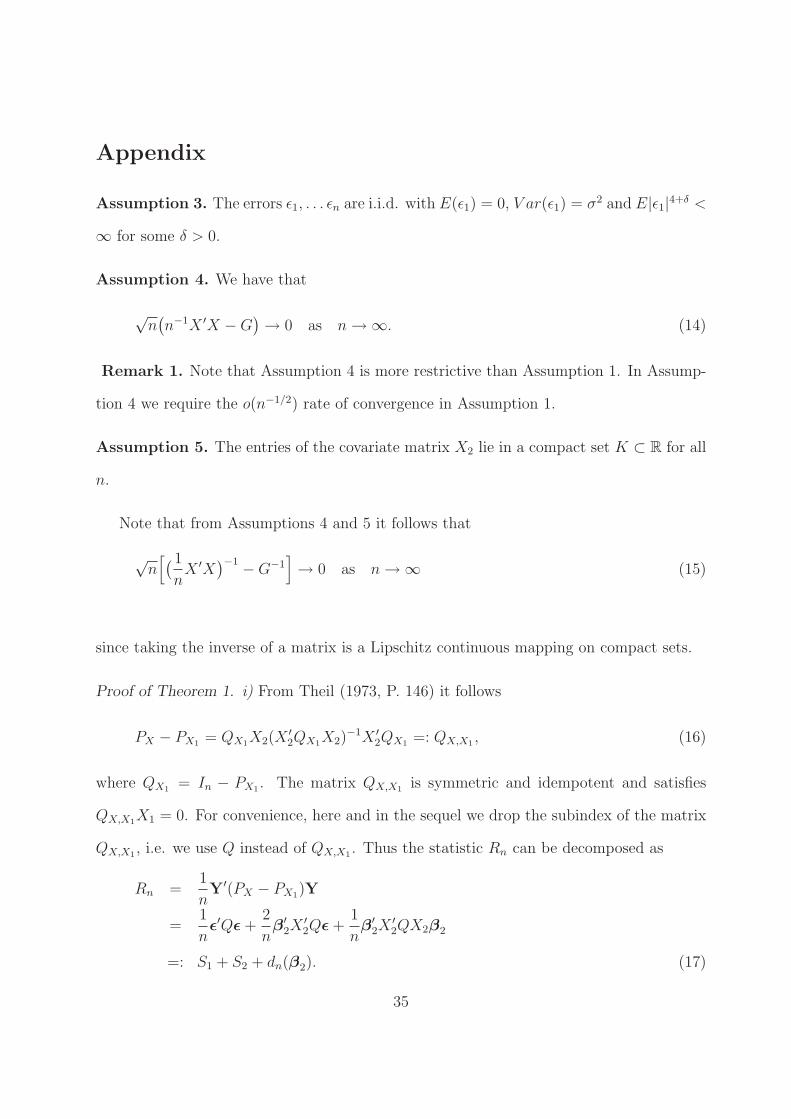
Assumption 3. The errors ǫ1, . . . ǫn are i.i.d. with E(ǫ1) = 0, V ar(ǫ1) = σ2 and E|ǫ1|4+δ <

∞ for some δ > 0.

Assumption 4. We have that

√n(

n−1X ′X − G)

→ 0 as n → ∞. (14)

Remark 1. Note that Assumption 4 is more restrictive than Assumption 1. In Assump-

tion 4 we require the o(n−1/2) rate of convergence in Assumption 1.

Assumption 5. The entries of the covariate matrix X2 lie in a compact set K ⊂ R for all

n.

Note that from Assumptions 4 and 5 it follows that

√n[

( 1

nX ′X

)−1 − G−1]

→ 0 as n → ∞ (15)

since taking the inverse of a matrix is a Lipschitz continuous mapping on compact sets.

Proof of Theorem 1. i) From Theil (1973, P. 146) it follows

PX − PX1= QX1

X2(X′2QX1

X2)−1X ′

2QX1=: QX,X1

, (16)

where QX1= In − PX1

. The matrix QX,X1is symmetric and idempotent and satisfies

QX,X1X1 = 0. For convenience, here and in the sequel we drop the subindex of the matrix

QX,X1, i.e. we use Q instead of QX,X1

. Thus the statistic Rn can be decomposed as

Rn =1

nY′(PX − PX1

)Y

=1

nǫ′Qǫ +

2

nβ′

2X′2Qǫ +

1

nβ′

2X′2QX2β2

=: S1 + S2 + dn(β2). (17)

35

Noting that ES1 = σ2tr(Q)/n ≤ σ2q/n → 0 as n → ∞ and E(S2) = 0, the first statement

of Theorem 1 now follows from (5).

ii) First note that relationships (14) and (15) imply

√n(

dn(β2) − d(β2))

→ 0.

Since by assumption, d(β2) > 0, dn(β2) will be bounded away from 0 and we get

√n

Rn − d(β2)

2σ√

dn(β2)=

√n

1nY′(PX − PX1

)Y − dn(β2)

2σ√

dn(β2)+ o(1). (18)

Consider now decomposition (17) for Rn. By virtue of Theorem 1.6 from Seber & Lee

(2003), the variance of the first term S1 in (17) is given by

V ar (S1) =1

n2

[

(µ4 − 3σ4)h′h + 2σ4tr(Q)]

,

where µ4 := E(ǫ41) and h is the vector of diagonal elements of the matrix Q, for which

h′h ≤ q2. Thus

S1 = OP (|ES1| + |S1 − ES1|) = OP (n−1).

Furthermore, ES2 = 0 and

V ar (S2) =4

n· σ2dn(β2) ∼

4

n· σ2d(β2),

and therefore the term S2 dominates the asymptotics in (17). It remains to show asymptotic

normality of S2. For this we check the Lyapounov condition

1

n(4+δ)/2

n∑

i=1

E |biǫi|4+δ =E|ǫ1|4+δ

n2+δ/2

n∑

i=1

|bi|3 → 0 as n → ∞,

where b′ := 2β′2X

′2Q = (b1, . . . , bn). It will be enough to show that the entries bi divided

36

by n are uniformly bounded. From Assumption 5 it follows that

maxi=1,...,n

|bi|n

=1

nmax

i=1,...,n|[QX2β2]i|

≤ 1

nmax

i=1,...,n

{

n∑

k=1

|[Q]ik| · |[X2β2]k|}

≤ C

nmax

i=1,...,n

{

n∑

k=1

|[Q]ik|}

,

where C > 0 and [ · ]ik denotes the (i, k)-th entry of the corresponding matrix. Since Q is

symmetric and positive semi-definite, |[Q]ik| ≤ (Qii + Qkk)/2, and thus

maxi=1,...,n

|bi|n

≤ C

nmax

i=1,...,n

{

1

2

n∑

k=1

([Q]ii + [Q]kk)

}

=C

nmax

i=1,...,n

{

n

2[Q]ii +

1

2tr(Q)

}

≤ C

n

n + 1

2tr(Q)

≤ Cq for n ≥ 1

This finishes the proof of Theorem 1.

Proof of Lemma 1. Using (10), (16) and noting QX1 = 0, we have

dn(β2,β3) =1

nβ′

2X′2QX1

X2β2 +2

nβ′

3X′3QX1

X2β2

+1

nβ′

3X′3QX1

X2(X′2QX1

X2)−1X ′

2QX1X3β3

=: T1 + T2 + T3. (19)

Consider T1 in (19). By virtue of Assumption 2 it follows that

T1 :=1

nβ′

2X′2QX1

X2β2

= β′2

(

X ′2X2

n− X ′

2X1

n

[

X ′1X1

n

]−1X ′

1X2

n

)

β2

→ β′2

(

G22 − G21G−111 G12

)

β2 as n → ∞

= β′2Aβ2.

37

Similarly, one can show that

T2 :=2

nβ′

3X′3QX1

X2β2

→ 2β′3

(

G32 − G31G−111 G12

)

β2

= 2β′3Bβ2 as n → ∞

and

T3 :=1

nβ′

3X′3QX1

X2(X′2QX1

X2)−1X ′

2QX1X3β3

→ β′3BA−1B′β3 as n → ∞.

Assumption 6. We have that

√n(

n−1Z ′Z − G)

→ 0 as n → ∞.

Remark 2. Note that Assumption 6 is more restrictive than Assumption 2. In Assump-

tion 6 we require the o(n−1/2) rate of convergence in Assumption 2.

Assumption 7. The entries of the covariate matrix [X2, X3] lie in a compact set K ⊂ R

for all n.

Sketch of proof of Theorem 2. Again using (16) we have

1

nY′(PX − PX1

)Y =1

nǫ′Qǫ +

2

nβ′

2X′2Qǫ +

2

nβ′

3X′3Qǫ + dn(β2,β3)

=: S1 + S2 + S3 + dn(β2,β3).

The term S1 is asymptotically negligible, and

Var(√

n(

S2 + S3

)

)

= 4σ2dn(β2,β3).

Now the proof of Theorem 2 is concluded similarly as the proof of Theorem 1.

38

model selection strategies for identifying most relevant - mediatum

Documents