modelare analiza element finit privind tensionarea benzii transportoqare
TRANSCRIPT

Northeastern University
Mechanical Engineering Master's Theses Department of Mechanical and IndustrialEngineering
May 01, 2012
Finite element analysis and a model-free control oftension and speed for a flexible conveyor systemZhan ZhangNortheastern University
This work is available open access, hosted by Northeastern University.
Recommended CitationZhang, Zhan, "Finite element analysis and a model-free control of tension and speed for a flexible conveyor system" (2012).Mechanical Engineering Master's Theses. Paper 70. http://hdl.handle.net/2047/d20003047

1
Finite Element Analysis and a Model-Free
Control of Tension and Speed for a Flexible
Conveyor System
A Thesis Presented
By
Zhan Zhang
To
Department of Mechanical and Industrial Engineering
In Partial Fulfillment for the Requirements
For the Degree of
Master of Science
In the field of
Mechanical Engineering
NORTHEASTERN UNIVERSITY
Boston, Massachusetts
Copyright May 2012 ©
NORTHEASTERN UNIVERSITY
Graduate School of Engineering

2
Thesis Title: Finite element analysis and a model-free
control of tension and speed for a flexible conveyor
system
Author: Zhan Zhang
Program: Mechanical Engineering
Approved for: Master of Science in Mechanical Engineering
Thesis Advisor: Abe Zeid Date
Thesis Advisor: Rifat Sipahi Date
Chairman of Department:
Graduate School Notified of Acceptance:
Associate Dean, Graduate and Research Programs:
Date
Copy deposited in library:
Reference Librarian

3
Abstract
In today's life, there is a wide variety of conveyor structures, from large heavy
load conveyor in modern mining industry to the conveyor belt with small and
simple structure in magnetic tape. Since its structure is simple, reliable and
easy to deploy, it has become one of the basic mechanical drive methods. But
almost every drive system suffers from fatigue failure, particularly the
conveyor belt itself. So how to analyze the stress in conveyor structure has
became a problem, which is worthy to study.
This thesis has two goals. First, we analyze the stresses in the conveyor belt
system to determine the maximum stresses in the belt to ensure system safety
during its operation. We build a 3D model of the system in Solidworks CAD
system. Then we build a finite element model of the system using tetrahedral
elements. We utilize nonlinear finite element analysis to calculate the stresses.
The analysis considers the material nonlinearity due to the belt rubber material.
Second, we derive a control algorithm to allow us to control the belt stress and
speed. We have used Simulink model of Matlab to build control a system. We
utilize the Kelvin-Voigt model, the Maxwell model and the Dzierzek model in
our simulation.
The results of both the computational finite element analysis and the control
simulation compare well with closed-form solutions. The maximum stress from
the finite element analysis is 16% off compared with the simple stress
calculations. This is attributed to the fact that we modeled the entire conveyor
belt system as assembly. The controller system results are within our
expectations. The speed and stress in the belt meet our desired goal of keeping
them constant via the control system.

4
Acknowledgements
First and foremost, I would like to express my most sincere gratitude to
my advisors Dr. Abe Zeid and Dr. Rifat Sipahi for the guidance and
patience. I thank them for teaching me all the skills necessary to complete
this journey.
I would like to thank my parents for their endless support and patience.
Without them I couldn’t have come this far. I thank them for always
being there for me.

5
Table of Contents
Acknowledgements
List of Figureures
List of tables
Introduction
1.1 Overview 1.2 Introduction to Simulink 1.3 CAD system 1.4 Components of conveyor system 1.5 Purpose and scope of research and research objectives
Chapter 2 Analysis of tape drive system
2.1 Overview of belt drive system 2.2 Belt drive analysis 2.3 Effective tension F 2.4 Slipping 2.5 Euler's formula 2.6 Stress analysis of belt drive
Chapter 3 – 3D Modeling of tape drive system
3.1 Components of tape drive system 3.2 Assembly method 3.3 Computational stress analysis of belt system 3.4 Analysis of simulation results
Chapter 4 – Control of tape drive system
4.1 Introduction to traditional PID control method 4.2 Introduction to ADRC 4.3 ADRC structure 4.4 Decoupled method for controlling the conveyor belt 4.5 Choices of modules
Chapter 5 –Simulation of tape drive system
5.1 Material model of conveyor system 5.2 Building ADRC in Simulink 5.3 Simulation Results 5.4 Putting the whole system together 5.5 Analysis of result
Reference

6
List of Figures
Figure 1.1 Simulink window
Figure 1.2 flat belt conveyor1
Figure 1.3 flat belt conveyor2
Figure 1.4 experiment model
Figure 2.1 conveyor structure
Figure 2.2 tension in the belt
Figure 2.3 tension in the belt work condition
Figure 2.4 centrifugal stress
Figure 2.5 bending stress
Figure 2.6 total stress
Figure 3.1 sketch of pulley
Figure 3.2 extrude pulley
Figure 3.3 chamfer
Figure 3.4 keyway
Figure 3.5 fillet1
Figure 3.6 fillet 2
Figure 3.7 sketch of hole
Figure 3.8 extrude cut hole
Figure 3.9 pattern the holes
Figure 3.10 pulley
Figure 3.11 sketch of base
Figure 3.12 extrude base
Figure 3.13 sketch of axis
Figure 3.14 extrude axis
Figure 3.15 components
Figure 3.16 pulley1 coincident mate1
Figure 3.17 pulley1 face coincident mate2
Figure 3.18 complete assembly
Figure 3.19 assembly features
Figure 3.20 create belt
Figure 3.21 conveyor assembly
Figure 3.22 feature selection
Figure 3.23 sketch selection
Figure 3.24 modifying status
Figure 3.25 extrude parameters
Figure 3.26 create belt
Figure 3.27 solid belt
Figure 3.28 open belt part
Figure 3.29 belt part
Figure 3.30 sketch on the belt
Figure 3.31 rectangle sketch

7
Figure 3.32 extrude cut
Figure 3.33 half belt
Figure 3.34 simulation study window
Figure 3.35 half belt assembly model
Figure 3.36 fixture on flat belt surface
Figure 3.37 fixture on circular arc belt surface
Figure 3.38 fixture on pulley
Figure 3.39 component contact
Figure 3.40 torque on belt contact surface
Figure 3.41 forces on the belt
Figure 3.42 torque on pulley
Figure 3.43 centrifugal force
Figure 3.44 mesh model
Figure 3.45 material window
Figure 3.46 simulation result
Figure 3.47 tight side stress
Figure 3.48 loose side stress
Figure 3.49 stress in the pulley
Figure 3.50 tight side stress
Figure 3.51 loose side stress
Figure 3.52 stress in the pulley
Figure 3.53 tight side stress
Figure 3.54 loose side stress
Figure 3.55 stress in the pulley
Figure 3.56 tight side stress
Figure 3.57 loose side stress
Figure 3.58 stress in the pulley
Figure 3.59 tight side stress
Figure 3.60 loose side stress
Figure 3.61 stress in the pulley
Figure 4.1 PID structure
Figure 4.2 global control
Figure 4.3 ADRC structure
Figure 4.4 poles’ location
Figure 5.1 Kelvin-Voigt model
Figure 5.2 Maxwell model
Figure 5.3 Dzierzek model
Figure 5.4 speed estimator structure
Figure 5.5 nonlinear combination
Figure 5.6 ADRC speed controller
Figure 5.7 tension estimator structure
Figure 5.8 nonlinear combination
Figure 5.9 ADRC tension controller
Figure 5.10 controller subsystems

8
Figure 5.11 tension test state-space window
Figure 5.12 tension controller test
Figure 5.13 tension controller test result
Figure 5.14 speed test state-space window
Figure 5.15 speed controller test
Figure 5.16 speed controller test result
Figure 5.17 Kelvin-Voigt model test
Figure 5.18 test result without filter
Figure 5.19 test result with filter
Figure 5.20 Maxwell model test
Figure 5.21 test result without noise
Figure 5.22 subsystem of Maxwell model
Figure 5.23 Maxwell model with noise
Figure 5.24 test result with noise
Figure 5.25 Dzierzek model
Figure 5.26 Dzierzek subsystem model
Figure 5.27 Dzierzek system with noise
Figure 5.28 Dzierzek system test result
Figure 5.29 Dzierzek system with filters
Figure 5.30 test result
Figure 5.31 Dzierzek with friction block
Figure 5.32 test result
Figure 5.33 Dzierzek with noise and friction blocks
Figure 5.34 test result
Figure 5.35 Maxwell model test result
Figure 5.36 Dzierzek model test result
Figure 5.37 Dzierzek model test result
Figure 5.38 Maxwell model test result
Figure 5.39 Maxwell model test result
Figure 5.40 Maxwell model test result

9
List of tables
Table 3.1 tight side and loose side forces

10
Introduction
1.1 Overview
In today’s world, industry has become the foundation of society. It is
important to keep industry improving. In the industry field, there are
several kinds of Transmission mechanisms, such as gears, cam, worm
gears and conveyors. Since the conveyor is suitable for the transmission
over large distance between two shafts centers, and it has a good
flexibility, when there is impact and vibrations on the conveyor, it could
reduce the effect of the impact and vibration [1]. Also when it is
over-loaded, the slipping effect will occur, and in this way, the other parts
will be protected. Considering the prices of all transmission mechanisms,
the conveyor is a cheap and reliable structure. With all above advantages,
the conveyor has become a widely used transmission method in all fields
of industry. So it is quite necessary for us to keep improving the methods
of analyzing the force in the belt and the way to control the conveyor
system.
Since there are varieties of conveyors in practice, the large conveyor
could be used in mining industry, and the small one could be used in
magnetic tapes. As a result we need a general model to analyze the
system. Also we could use this general model to develop various complex
models, which will be closer to real working conditions. This project

11
consists of two parts; one is using active disturbance rejection control
method to control speed and tension of the belt. The other part uses
Solidworks to build 3D model and apply finite element analysis on this
model.
In this thesis, based on a general flat belt conveyor system model [2-4], in
the control system design; the belt was treated as a thin belt, which means
only the tension was considered. In the 3D finite element model, the belt
could be analyzed with different materials and boundary conditions to see
the changes of stress and strain, so that we could judge the best material
and operating conditions for the conveyor and build a control system to
control it.
1.2 Introduction to Simulink
Simulink is an important component of Matlab; it provides an
environment of dynamics system modeling, simulation and a
comprehensive analysis. It is a visual simulation tool in Matlab, and also
a package based on Matlab block diagram design environment. Simulink
is widely used in the modeling and simulation of linear and nonlinear
systems, digital control and digital signal processing. In Simulink, the
sample time could be defined as discrete sampling time or continuous
sampling time. It also supports multi-rate system, where different parts
have different sampling time. To build a dynamic system, Simulink offers

12
a graphical user interface (GUI) to model the block diagram; the process
could be done by simply clicking and dragging the mouse. It provides a
fast, straightforward manner, and the user can immediately see the
simulation results of the system.
The Simulink has following characteristics: rich expansion predefined
module library; interactive graphics editor to combine and intuitive
manage module diagram.
There are two ways to run the Simulink:
1. Type Simulink in the MATLAB command window
There will be a window called Simulink Library Browser (Figure 1.1); all
the blocks are listed in this window.
Figure 1.1 Simulink window

13
2. Click the quick link button on MATLAB main window
There are 8 Sub-libraries, classified by their functions, in Simulink:
Continuous, Discrete, Function &Tables, Math,Nonlinear,Signals
&Systems,Sinks,Sources. We could choose necessary blocks to build the
desired system.
1.3 Solidworks CAD system
Solidworks is mechanical design software which contains varieties of
components and functions. It is also the first three-dimensional CAD
software which is developed based on Windows system. For the users
who are familiar with Microsoft’s Windows system, basically they can
use Solidworks to begin designing jobs.
Here are some key advantages of Solidworks:
·Solidworks provides a complete set of dynamic interface, and
drag-mouse control method. The “full dynamic” user interface reduces
design steps, and improves the designer experience.
·The intelligent assembly technology [5] which is called capturing mate is
used in Solidworks to speed up the general assembling process. The
intelligent assembly technology means that Solidworks could
automatically capture and define assembly relationships.
·With Solidworks, we could view all the dynamic movements of moving
parts in the assembly. We could also make dynamic interference checking

14
and gap detection.
·With all the advantages, Solidworks is the best option for us to perform
analysis of the conveyor system.
1.4 Components of conveyor system
The conveyor system is always divided into two parts: pulleys connected
by traction pieces. This kind of conveys always include traction pieces,
carrier components, drive units, tensioning device, redirecting means,
support member, etc.
Traction pieces can be used to transfer traction, they can be conveyor belt,
traction chain or wire rope. Carrier components are used to hold the
materials we want to transfer; they could be hopper, bracket or spreader.
The drive unit is used to transmit power; it is usually consisted of electric
motor, reducer and brake. The tensioning device is generally divided into
two kinds, one is screw type and the other is heavy hammer type; it is
used to maintain a certain tension in the belt. So the conveyor could
transmit power at maximum efficiency. The support member is used for
supporting traction members; it can be roller or pulley.
The structure characters of a conveyor device having a traction member is
that, the material need to be transported is mounted on the supporting
members which are linked with the traction member, or directly mounted
on the traction member (such as conveyors). Traction members bypass

15
connect to both of the respective rollers or sprockets, including the
formation of transportation of materials with a closed loop of the load
branch and no-load transportation of materials branch. The structures are
shown in Figure 1.2 and Figure 1.3
Figure 1.2 flat belt conveyor1
Figure 1.3 flat belt conveyor2
The conveyor system is too complex to study, so we ignore some parts in
our study; we only focus on the belt and the pulleys, shown in Figure 1.4.

16
Figure 1.4 experiment model
We could make the model more complex according to different working
conditions and different types of conveyors by changing the dimensions
of pulleys and motors. Also we could change the math model of conveyor
to make it become more realistic.
1.5 Purpose and scope of research and research objectives
Our purpose is to design a control system with the help of Simulink to
control the speed and tension in the conveyor belt. Another goal is to
build 3D model in Solidworks to apply finite element analysis on the
model to check the stress and strain in the belt and make comparison with
different loading conditions.

17
Chapter 2 Analysis of tape drive system
2.1 Overview of belt drive system
Belt drive system consists of two pulleys and a belt tightly wrapped
around them. Relying on the friction between the contact surfaces of the
belt and pulley to transmit motion and power, it is a flexible frictional
transmission as shown in Figure 2.1.
Figure 2.1 conveyor structure
2.2 Belt drive analysis
Figure 2.2 shows the belt forces on both sides of the belt in static
conditions, i.e. the belt is not working, when the belt moves, it has a tight
side and a loose side. The tight side tension F1 increasing from F0 to F1;
The loose side tension is F2 decreasing from F0 to F2
Figure 2.2 tension in the belt

18
Assuming the total length of the belt will not be changed, the tight side
tension incremental F1 - F0 should be equal to the amount of decrease of
the slack side tension F0 - F2.
2.3 Effective tension F
Effective tension F is the effective circumferential force the belt drive can
transfer effectively. It is not the concentrated force acting in a fixed point,
but the sum of the friction generated by the contact surface of the belt and
pulley, i.e.
0 1 2
1 2
1( )
2F F F
F F F
(2.1)
1 ,2
FF F
22
FF F
The relationship between the circumferential force F (N), the belt speed v
(m / s) and the transmission power P (KW):
1000
FvP
(2.2)
2.4 Slipping
When the desired delivery circumferential force exceeds the friction force
between the belt and the tread, sliding between the belt and the pulley
occurs, a phenomenon called slip. The wear of the belt will often
aggravate slipping and reduce the transmission efficiency, resulting in

19
drive failure.
2.5 Euler's formula
The relationship between the tension forces F1 and F2 on both sides of the
belt are given by the following Euler’s formula:
1 2
fF F e (2.3)
Where: f is the coefficient of friction between the belt and the wheel
surface; α is the Wrap angle (rad); e is the natural logarithms (e ≈ 2.718).
The above equation is the basic flexible friction formula, known as
Euler’s formula. The belt forces are shown in Figure 2.3.
Figure 2.3 tension in the belt work condition
2.6 Stress analysis of belt drive
We use flat belts as an example. When the belt is moving, the stress in the
belt is composed of the following three parts:
(1) Tight side and loose side tensions generate tensile stresses
Tight side tensile stress:
11
F
A (2.4)

20
Loose side tensile stress:
22
F
A (2.5)
A is the cross-sectional area of the belt (mm2).
(2) Tensile stress caused by Centrifugal force
Centrifugal tensile stress is given by Equation (2.6), and shown in figure
2.4.
2
cc
F qv
A A ( 2.6 )
Figure 2.4 centrifugal stress
(2) Bending stress, shown in figure 2.5. The stress is given by Equation
(2.7)
2b
yE
D (2.7)

21
Figure 2.5 bending stress
Where: y is the vertical distance (mm) of neutral layer of the tape to the
outermost layer; E is the modulus of elasticity of the belt material (MPa);
d is the pulley diameter (for the V-belt pulley, d is the standard diameter.)
Figure 2.6 total stress
Based on the above analysis, while belt is transferring forces, there are
three kinds of stresses in the belt: tensile stress, Centrifugal tensile stress,
and bending stress. As shown in figure 2.6, the maximum stress occurs
around the tight side at the small pulley. The maximum stress value is:

22
1 b ct (2.8)
So while the belt drive system is running, the maximum location stress
varies. This means the belt works under varying stress. When the number
of stress cycles reaches a certain value, the fatigue failure will occur.

23
Chapter 3 – 3D Modeling of tape drive system
3.1 Components of tape drive system
3.1.1 Design of pulley
Since the model is based on the flat band, to make the study more
realistic, the 3D model is drawn according to the design process of flat
band pulley.
Step 1, according to relative calculation and background; draw the sketch,
shown in Figure 3.1.
Figure 3.1 sketch of pulley
24
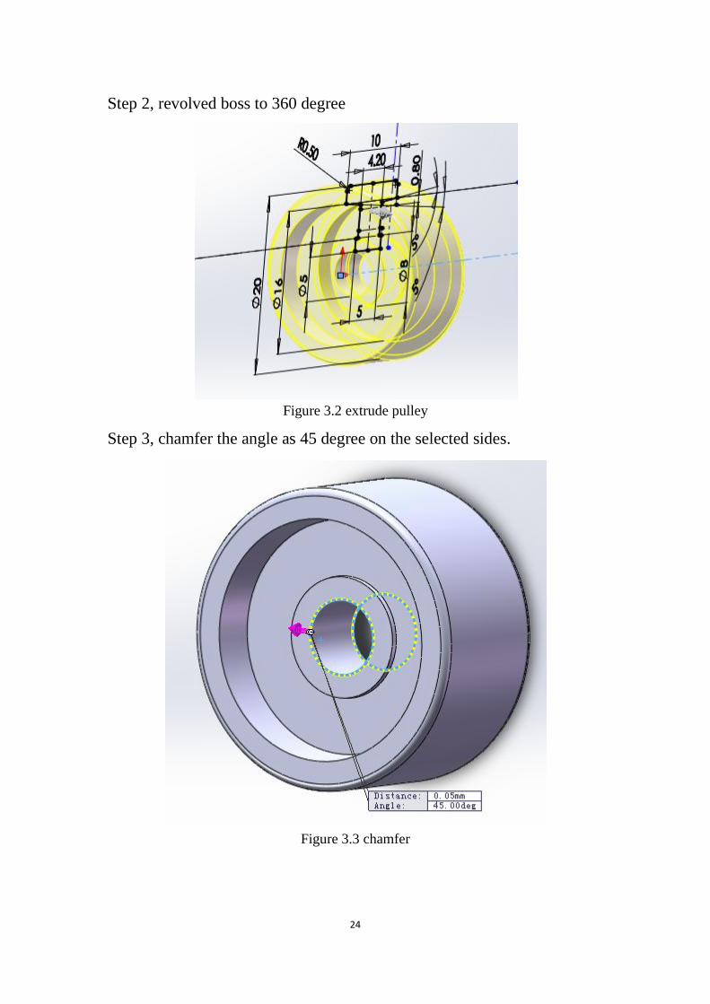
Step 2, revolved boss to 360 degree
Figure 3.2 extrude pulley
Step 3, chamfer the angle as 45 degree on the selected sides.
Figure 3.3 chamfer
25
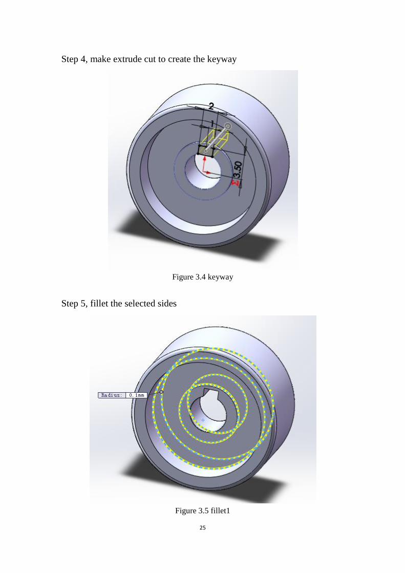
Step 4, make extrude cut to create the keyway
Figure 3.4 keyway
Step 5, fillet the selected sides
Figure 3.5 fillet1

26
Figure 3.6 fillet 2
Step 6, draw the sketch on the face of pulley
Figure 3.7 sketch of hole

27
Step 7, extrude cut , through all bodies
Figure 3.8 extrude cut hole
Step 8, circular pattern as shown below
Figure 3.9 pattern the holes

28
Step 9, review the pulley 3D CAD model
Figure 3.10 pulley
3.1.2 Base design
The function of base is to make sure the pulleys move in the same way as
they did under real operating conditions. So the structure is simple. And
when we create simulation, we could exclude the base from the study.
Step 1, Draw the base sketch
Figure 3.11 sketch of base

29
Step 2, Extrude the sketch
Figure 3.12 extrude base
Step 3, Draw the circle sketch on the base face
Figure 3.13 sketch of axis
Step 4, Extrude the sketch a distance of 15mm
Figure 3.14 extrude axis

30
3.2 Assembly method
(1) Insert 2 pulleys and the base in the assembly model
Figure 3.15 assembly components
(2) Mate the two selected faces as coincident
Figure 3.16 pulley1 coincident mate1

31
(3) Make the two faces coincident
Figure 3.17 pulley1 face coincident mate2
(4) Repeat the same step for the other pulley
Figure 3.18 complete assembly
(5) Add relationship between two pulleys. Since it is belt drive system,
we need to choose Belt/Chain option

32
Figure 3.19 assembly features
(6) Choose parameters of belt, such as the face the belt is mounted on
Figure 3.20 create belt
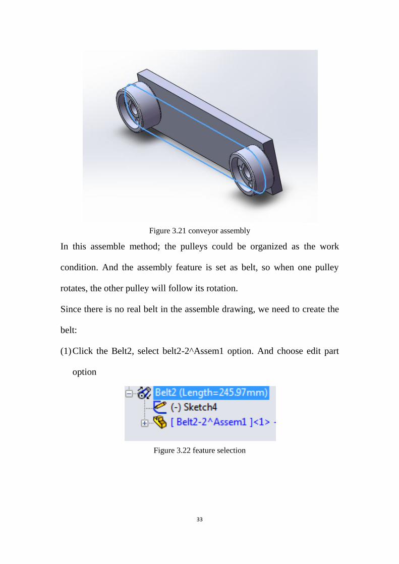
(7) Add a thickness of 1mm to the belt
33
Figure 3.21 conveyor assembly
In this assemble method; the pulleys could be organized as the work
condition. And the assembly feature is set as belt, so when one pulley
rotates, the other pulley will follow its rotation.
Since there is no real belt in the assemble drawing, we need to create the
belt:
(1) Click the Belt2, select belt2-2^Assem1 option. And choose edit part
option
Figure 3.22 feature selection

34
(2) Select Sketch2
Figure 3.23 sketch selection
Figure 3.24 modifying status
(3) Extrude the sketch. The parameters are set as shown
Figure 3.25 extrude parameters
35
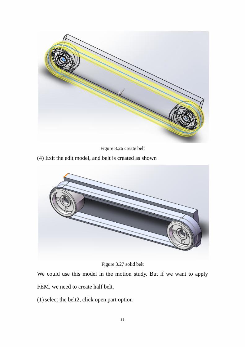
Figure 3.26 create belt
(4) Exit the edit model, and belt is created as shown
Figure 3.27 solid belt
We could use this model in the motion study. But if we want to apply
FEM, we need to create half belt.
(1) select the belt2, click open part option

36
Figure 3.28 open belt part
Figure 3.29 belt part
(2) Sketch rectangle on the selected face to cut the belt by half to enable
us to perform stress analysis using the finite element method.
Figure 3.30 sketch on the belt
37
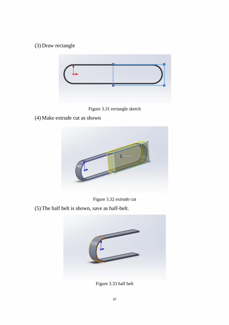
(3) Draw rectangle
Figure 3.31 rectangle sketch
(4) Make extrude cut as shown
Figure 3.32 extrude cut
(5) The half belt is shown, save as half-belt.
Figure 3.33 half belt
38
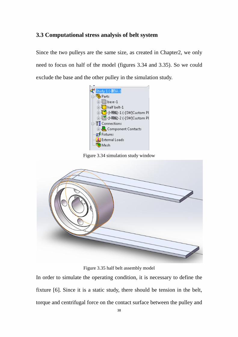
3.3 Computational stress analysis of belt system
Since the two pulleys are the same size, as created in Chapter2, we only
need to focus on half of the model (figures 3.34 and 3.35). So we could
exclude the base and the other pulley in the simulation study.
Figure 3.34 simulation study window
Figure 3.35 half belt assembly model
In order to simulate the operating condition, it is necessary to define the
fixture [6]. Since it is a static study, there should be tension in the belt,
torque and centrifugal force on the contact surface between the pulley and

39
the belt. Since the pulley could rotate around the axis, and the belt will be
tight, so the fixture could be defined as:
(1) The bottom side of the belt is set as roller/slider fixture.
Figure 3.36 fixture on flat belt surface
(2) The contact surface between the pulley and the belt is set as fixed
geometry
Figure 3.37 fixture on circular arc belt surface
(3) Since the pulley could rotate around the axis, the pulley is set as fixed
on the cylindrical faces, and circumferential sub option, but the study is

40
static, so the rotation angle is set as zero.
Figure 3.38 fixture on pulley
(4) We also need to define the component contact to make sure there
would be contact fore between the pulley and the belt.
Figure 3.39 component contact
Next step, we need to apply external loads on the model.
(1) Apply 2 NM torque on the contact surface
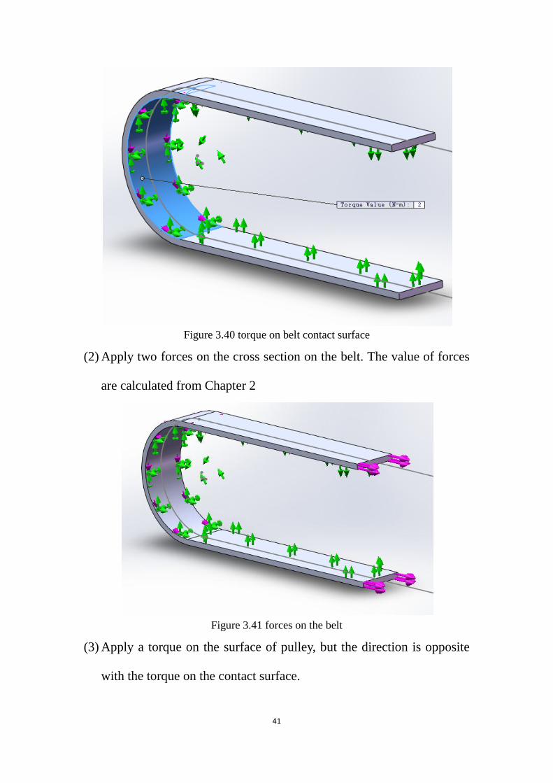
41
Figure 3.40 torque on belt contact surface
(2) Apply two forces on the cross section on the belt. The value of forces
are calculated from Chapter 2
Figure 3.41 forces on the belt
(3) Apply a torque on the surface of pulley, but the direction is opposite
with the torque on the contact surface.

42
Figure 3.42 torque on pulley
(4) Apply centrifugal force on the inter surface. Suppose the angular
velocity is 2 rad/s.
Figure 3.43 centrifugal force
(5) Create the finite element mesh. The mesh method is selected as
Jacobian 4 points model

43
Figure 3.44 mesh model
The last step is to define different materials of different parts in the
model.
(1) Define the belt as rubber, and define the pulley as alloy steel. We
could choose the materials from Solidworks material list.
Figure 3.45 material window

44
(2) Run the simulation
Figure 3.46 simulation result
3.4 Analysis of simulation results
We use the equations shown in Chapter 2. Suppose the tight side tension
is 2N, we could calculate the loose side force:
1 2
fF F e (3.1)
In this model the wrap angle is 0180 , which is described as in rad. And
according to related information, the friction coefficient f is 1. So here is
the calculation result:
Table 3.1 tight side and loose side forces
F1(N) 2 5 10 15 20
F2(N) 0.08 0.2 0.4 0.6 0.8
It is obvious that the loose side tension is very small compared with tight
side tension. Since the pulleys are rotating, there should be centrifugal
force in the belt. The friction force appears as torque on the contact
45
surface.
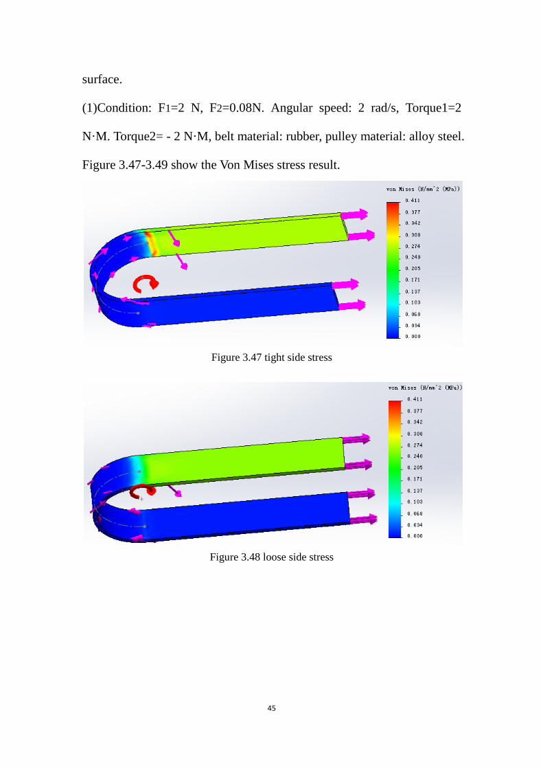
(1)Condition: F1=2 N, F2=0.08N. Angular speed: 2 rad/s, Torque1=2
N·M. Torque2= - 2 N·M, belt material: rubber, pulley material: alloy steel.
Figure 3.47-3.49 show the Von Mises stress result.
Figure 3.47 tight side stress
Figure 3.48 loose side stress

46
Figure 3.49 stress in the pulley
According to the Figures, the belt max stress occurs on the the tight side
of the belt where the belt wraps around the pulley.
According to Equation (2.6) in Chapter 2, the max stress is:
max 1 b c .
So we could get the value of max stress that:
1
0
2
max
20.25
8
2 2 0.50.61
10
4 0.010.004
8
0.864
b
c
FMpa
A
Ey EMpa
d
qvMpa
A
Mpa
(3.2)
The max stress is about 1Mpa, according to Figure. 3.47. Comparing the
manual calculation result and the simulation result, we get the error:
max max
max
0.864 0.411100% 100% 52.4%
0.864
fem manual
error

47
(2) Condition: F1=5 N, F2=0.2N, angular speed: 2 rad/s, torque1=5 N·M,
torque2= - 5 N·M, belt material: rubber, pulley material: alloy steel. The
stress result are shown in figure (3.50-3.52).
Figure 3.50 tight side stress
Figure 3.51 loose side stress

48
Figure 3.52 stress in the pulley
The max stress still obeys the rule, and the value increases significantly.
According to max stress Equation (2.6) in Chapter 2, we get the following
result:
1
0
2
max
51.25
8
2 2 0.50.61
10
4 0.010.004
8
1.239
b
c
FMpa
A
Ey EMpa
d
qvMpa
A
Mpa
(3.3)
The max stress is about 1Mpa, according to Figure. 3.50. Comparing the
manual calculation result and the simulation result, we could get the
error:
'
max max
max
1.239 1.05100% 100% 15.3%
1.239error

49
(3)Condition: F1=10 N, F2=0.4N, angular speed: 2 rad/s, torque1=10
N·M, torque2= - 10 N·M, belt material: rubber, pulley material: alloy
steel. Stress results are shown in figure (3.53-3.55).
Figure 3.53 tight side stress
Figure 3.54 loose side stress
50
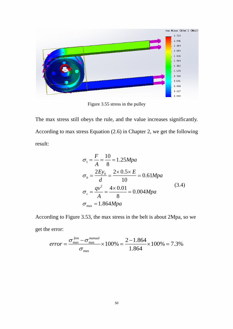
Figure 3.55 stress in the pulley
The max stress still obeys the rule, and the value increases significantly.
According to max stress Equation (2.6) in Chapter 2, we get the following
result:
1
0
2
max
101.25
8
2 2 0.50.61
10
4 0.010.004
8
1.864
b
c
FMpa
A
Ey EMpa
d
qvMpa
A
Mpa
(3.4)
According to Figure 3.53, the max stress in the belt is about 2Mpa, so we
get the error:
max max
max
2 1.864100% 100% 7.3%
1.864
fem manual
error

51
(4)Condition: F1=15 N, F2=0.6N, angular speed: 2 rad/s, torque1=15
N·M, torque2= - 15 N·M, belt material: rubber. Pulley material: alloy
steel. The stress results are shown in figure(3.56-3.58).
Figure 3.56 tight side stress
Figure 3.57 loose side stress
Figure 3.58 stress in the pulley

52
According to max stress Equation (2.6) in Chapter 2, we get the following
result:
1
0
2
max
151.875
8
2 2 0.50.61
10
4 0.010.004
8
2.489
b
c
FMpa
A
Ey EMpa
d
qvMpa
A
Mpa
(3.5)
According to the simulation result, the max stress in the belt is about
2.9Mpa, so there will be an error:
'
max max
max
2.9 2.489100% 100% 16.5%
2.489error
(5)Condition: F1=20 N, F2=0.8N, angular speed: 2 rad/s, torque1=20
N·M, torque2= - 20 N·M, belt material: rubber. Pulley material: alloy
steel. The stress results are shown in figure(3.59-3.61).
Figure 3.59 tight side stress
53
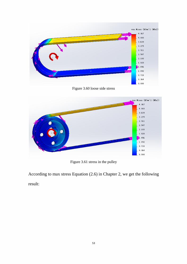
Figure 3.60 loose side stress
Figure 3.61 stress in the pulley
According to max stress Equation (2.6) in Chapter 2, we get the following
result:

54
1
0
2
max
202.5
8
2 2 0.50.61
10
4 0.010.004
8
3.1
b
c
FMpa
A
Ey EMpa
d
qvMpa
A
Mpa
(3.6)
In the simulation result, the max stress in the belt is around 3.3Mpa, so
we could get the error:
max max
max
3.8 3.1100% 100% 20%
3.1
fem manual
error

55
Chapter 4 – Control of tape drive system
4.1 Introduction to traditional PID control method
Since PID theory is developed long time ago, it is limited by the
technology level at that time [7-9]; it could not be applied with advanced
digital signal processing technology. But the PID controller is able to
handle most problems, and as a main theory in the engineering control
field.
The basic structure of PID [10] is shown in Figure 4.1.
Figure 4.1 PID structure
There are several incompletions [11-13] of PID control:
(1) The error is generated by e v y directly [10]. Our control goal is
that v could be drastically changed, but the output of object y has
inertia, so y could not be drastically changed, but slowly. In this way,
applying the slowly changed variable y to track drastically changed
variable v is not rational.
(2) There is no good way to generate differential signal of error de
dt

56
since differentiation could be obtained only with approximation
( ) ( )v t v ty
where tau can be seen as the sampling period.
Differentiation could also cause problems with noisy signals. When
the input signal ( )v t is affected by noise, the approximated
differential ( ) ( )v t v t
y
, in the output y will be affected by the
noise component as( )n t
, which amplifies as goes to a small
number. To prevent this, a low pass filter could be used, rendering the
derivative operation transfer function as 01
sy v
s
, where 0 is the
time constant of the filter producing a cut-off frequency at 1
in
frequency domain Although the output y can be made less affected
from noise, the value of 1
determines the bandwidth, and some
sacrifice is needed in system’s bandwidth to be able to obtain a
differential of a noisy signal with minimal effects due to noise.
(3) There are several disadvantages to applying the feedback of
integration of error signal in the form of 0
( )e d
. Feedback law
utilizing the signal feedback make is in general known to make the
closed loop response slower and prone to oscillations due to induced
low damping ratio.

57
(4) According to the PID control theory, we need to know the entire
open loop character equations. But sometimes the entire open loop
character equations are difficult to get. So we need to find a new way
to build control system.
4.2 Introduction to ADRC
Active Disturbance Rejection Control (ADRC) [14] is a new method to
build a control system around a plant, model of which is unknown. This
method is also based on the error feedback, which can be seamed together
with a PID controller.
In general, control systems have a structure as shown in Fig 4.2, where v
is the reference, and the controller uses both the reference and the output
of the plant, to produce the control action u to be applied on the plant.
Importantly, here the mathematical model of the plant is known, so that a
proper controller can be designed for it.
Figure 4.2 global control
In this traditional approach, the control parameters are selected based on
the open loop differential equation, e.g. given by ( , )dx
x f xdt
, where the
function f is known, and the state variables are x and dx
dt.
y

58
So if we want to control the system described above, we need get the
information about the open loop dynamics ( , )dx
f xdt
and the state variables
,dx
xdt
. But actually this could not be done, for the reason that in real world,
there is seldom information about the open loop dynamics, and in some
cases the open loop is too complex that its modeling is prohibitive.
Therefore, in such situations, the classical control design approached
cannot be directly applied to control the open loop system.
In fact, to achieve the control goal does not mean we need to know the
open loop dynamics of the system, as argued by Han [14] in his work on
ADRC. For example, consider the second order dynamics given by:
( , )dx
x f x udt
y x
(4.1)
Where u is the input, function ( , )dx
f xdt
is unknown, state variables are
,dx
xdt
, and y is the measurement.
The main idea behind model-free control for achieving the control goal is
to reduce the error between the desired value ( )v t and the output of the
system y, by regulating the input ( )u t into the system. So what we need
to know is the specific value of the open loop dynamics in the control
process, but not necessarily the explicit definition of the function f. We
suppose this value is
( ) ( ( ), )dx
a t f x tdt
(4.2)

59
According to Equation (4.1), ( )a t could be expressed as
( )a t x u (4.3)
So if we know input u and output y x , we could calculate ( )a t from
Equation (4.3) by carefully differentiating x twice.
In this way, once ( )a t is at hand, the control signal ( )u t can be
adjusted as:
0( ) ( )u t a t u (4.4)
After this basic transformation, the differential equation of the closed
loop system becomes a linear process:
2
02( )
d yu t
dt (4.5)
Then the control signal 0 ( )u t can be designed using a PID-like block on
the error e and differential error e v y as:
2
0 1 0 2( )
d edeu t a e a
dt dt
(4.6)
Finally, the closed loop equation becomes:
2
1 02
d e dea e a
dt dt (4.7)
Obviously, this differential equation is stable as long as 0a and 1a are
positive quantities, ( ) 0e t , so we could achieve the control goal
( ) ( )y t v t .
This control method approach that underlies the main idea behind
model-free control is different from the classical control design approach

60
as it does not rely on mathematical model of the open loop system. it is
mainly based on signal processing of input-output signals, and estimating
the “dynamic load” ( )a t , to produce control actions using ( )a t to be
able to attain the control objective. It is important to note here that the
estimation of ( )a t should be instantaneous, and preferably noise free,
and the open loop system, either linear or nonlinear, should have some
smoothness properties [10].
4.3 ADRC structure
Here y which is measurable is the output to be controlled, u is the input,
and open loop nonlinear system is described by an unknown function
1 2( , , ( ), )f x x w t t , which is in general a function of states, external
disturbances and time.
Suppose the system is given by:
12
1
21 2( , , ( ), )
dxx
dt
y x
dxf x x w t t bu
dt
(4.8)
According to ADRC theory, we do not need to know 1 2( , , ( ), )f x x w t t
specifically, and the open loop system can still be controlled as we
summarize next. First sets 1 2( , , ( ), )f x x w t t as 3x , and
1 2( , , ( ), )( )
df x x w t tG t
dt , so the whole system could be described as:

61
12
23
3
1
( )
dxx
dt
dxx bu
dt
dxG t
dt
y x
(4.9)
Then constructs a state observer, known as the extended state observer
(ESO).
1
12 01
23 02
303
e z y
dzz e
dt
dzz bu e
dt
dze
dt
(4.10)
To predict the numerical value of 3 1 2( ) ( , , ( ), )x F t f x x w t t . In this ESO,
the input is the system output y and control signal u.
So the system equations become:
1
12
20
1
e z y
dxx
dt
dxu
dt
y x
(4.11)
Figure 4.3 shows the ADRC architecture.

62
Figure 4.3 ADRC structure
Since the control goal is for instance to maintain a constant force in the
tension of the conveyor belt, and a constant speed of conveyor belt, we
could let the two control signals V1 and V2 as 12
dvv
dt . See Fig 4.3.
4.4 Decoupled method for controlling the conveyor belt
From figure 1.4, the equations of motion of the conveyor belt system can
be developed as:
2
112 e m
dJ T r K i
dt
(4.12)
2
222 e m
dJ T r K i
dt
(4.13)
2 12 1( ) ( )e
dx dxT k x x b
dt dt (4.14)
1 23
( )
2
x xx
(4.15)
What we need to control is the tension Te and the velocity 3dx
dt, by
applying control signals to the two motors. Assuming the above model is
actually not available, we will apply the ADRC scheme to the control

63
problem described above. For this, we will demonstrate how ADRC
applies to the system in the decoupled form. We know that the plant at
hand could be uncoupled and treated as two independent second-order
system. One is for X3 and the other one is for Te.
To accomplish the uncoupling, note equal commands on the two current
inputs. One will cause the tension, but no change in X3, the other will
cause a change in X3, but no effect on tension Te. So suppose:
3 1
2
1 1
1 1d
t
u iU
u i
(4.16)
We could get the transform matrix:
1 1
1 1uT
(4.17)
We also need to define a new state. What we need is X3 and tension Te, so
the new state should include X3, tension Te and its derivatives, i.e.
3
3
d
e
e
X
dX
dtX
T
dT
dt
(4.18)
We already know the system matrix:
1
2
1
2
0 0 10 0
0 0 0 10
3.315 3.315 0.5882 0.5882
3.315 3.315 0.5882 0.5882
d
X
XX

64
1
2
0 0
0 0
8.533 0
0 8.533
i
i
(4.19)
And the state matrix before the decoupling modification is given by:
1
3 2
1
2
0.5 0.5 0 0
2.113 2.113 0.375 0.375e
x
x xx
T
(4.20)
In which, we define two transformation matrices:
3 0.5 0.5 0 0H (4.21)
2.113 2.113 0.375 0.375tH (4.22)
So the new state could be expressed as:
3
3
d d
t
t
H
H Fx x T x
H
H F
(4.23)
So we can write the new state-space equation:
dd d d d
dxF x G U
dt (4.24)
Where
1
d d dF T FT and 1
d d uG T GT (4.25)
As we run the calculations in Matlab, and we get:

65
0 0
42.7 0
0 3.2
0 176.5
dG
and
0 1 0 0
0 0 0 0
0 0 0 1
0 0 66.3 1.18
dF
(4.26)
In this way, the system has been decoupled into two separate systems.
3
3
332
3
2
0 1 0
0 0 42.7
d xx
dtud x
d xdt
dt
(4.27)
And 2
2
0 1 3 . 2
6 6 . 3 1 . 1 8 1 7 6 . 5
e
e
te
e
d TT
dtud T
d Tdt
dt
(4.28)
The two system equations could be used to design a control system as if
the plant is composed of two decoupled single input single output
dynamics.
4.5 Choices of modules
In this section, we discuss how to choose the parameters in ADRC
controllers.
4.5.1 Kp Ki Kd controller gains in the tension controller
According to ADRC theory, the tension system could be described as:

66
12 1
23 2
3
d xx b u
dt
d xx b u
dt
d xG
dt
(4.29)
3x is the state we do not know, and we set 0 3
2
u xu
b
, so the system
equation becomes:
1 12 0 3
2
20
( )d x b
x u zdt b
d xu
dt
(4.30)
Notice that only X1 and X2 are the variables we want to control. And the
input U0 should be based on the error of estimated value and desired
value. So we define U0 as:
1 10 1 1 2 2
( )( ) ( )i
p d
K x zu K x z K x z
s
(4.31)
Since z1, z2, z3 are the disturbances, we could ignore them in the stability
calculation. Taking U0 into the system equation, and applying the values
b1=3.2 and b2=176.5, we could get the following characteristic equation:
3 20.020.02
00.02 1 0.02 1 0.02 1
p id i i
d d d
K KK K Ks s s
K K K
(4.32)
Since there are three variables in the equation, it is difficult to apply
Routh’s stability criterion. Root locus could be easier to implement for
studying stability of Equation (4.32). As we know, the settling time is

67
based on dominant poles is 4/ n , which we can use to make sure the
system response is fast and has sufficient damping.
For the 3rd
system in Equation (4.32), we need to choose 3 poles. We start
the pole locations at -3, 5 3i , and use them in Equation (4.32) to find
out the controller gains, which are found as kd=100, ki=102. We next
relax the Kp gain to explore if we can improve the system performance
determined by the dominant poles. For this, we re-write Equation (4.32)
in root locus form with respect to the parameter Kp
2
3 2
(0.02 )1
100 2.04 102
pK s s
s s s
(4.33)
We then plot the root locus in Matlab:
Figure 4.4 poles’ locations of the root locus form in Equation (4.33)
According to the Figure 4.4, it is obvious the poles are all on the left side
of the Imaginary axis, which means the system is stable. We could choose
a better Kp on the root locus by dragging the poles location. In this case,

68
we choose Kp =2930.
Finally, the parameters should be:
2930
100
102
p
i
d
K
K
K
Which locates the closed loop poles at: 49.98 17.81, 0.04
4.5.2 Kp Ki Kd selection speed controller
Compared with tension controller, speed control is relatively easier. The
system equation is:
12
1
2
d xx bu
dt
y x
d xG
dt
(4.34)
Assume the control signal is:
0 1 1( )( )ip d
Ku K K s x z
s (4.35)
Take U0 into system equation, we get:
2( 1) 0d p iK s K s K (4.36)
Suppose the poles are at 4 4i , then we get:
1
4
1.125
p
i
d
K
K
K
4.5.3 Controller design of the Estimator in tension controller
Bet4 bet5 bet6 determine the stability and speed of the estimator, which
directly affects the success of control. In the estimator, the system
equations are given by:

69
12 4
23 5
36
d zz bu e
dt
d zz e
dt
d ze
dt
(4.37)
The states that need to be stabilized are z1, z2 and z3, so we need to treat
control signal u and output y as disturbance. Transform the system
equations into matrix form:
1
1 4
22 5 1
3 6
3
0 1 0
0 0 1 ( )
0 0 0
d z
dtz
d zz z y Disturbance
dtz
d z
dt
(4.38)
Next exclude the output y as it is the non-homogeneous part of Equation
(4.38), and apply Laplace transformation on the homogeneous terms to
get the eigenvalue problem:
4
5
6
1 0
1
0
s
sI M s
s
(4.39)
Which leads to the following characteristic equation:
3 2
4 5 6 0s s s (4.40)
To make sure this system is stable, suppose the poles are all -10, take the
poles into equation, to calculate the beta values by comparing Equation
(4.40) with the following equation:

70
3 230 300 1000 0s s s (4.41)
From which we get:
4
5
6
30
300
1000
4.5.4 Controller gains in the Estimator for speed controller
In the speed control problem, the estimator is a 1st order system,
12 1
22
d zz bu e
dt
d ze
dt
(4.42)
Treat output y and control signal u as disturbance, and transform the
system equation into matrix form:
1
1 1
1
2 22
0 1
0 0
d z
dt zz Disturbance
zd z
dt
(4.43)
Make Laplace transformation on the homogeneous terms only to get the
following eigenvalue problem:
1
2
1ssI M
s
(4.44)
Then we suppose that two poles of the estimate are both at -1. Which
re-writes as:
2 2 1 0s s (4.45)
From which we get: 1
2
2
1
After all the parameters are chosen, the two ADRC controllers should be

71
stable. Since the controllers are independent from the plant, we could
apply the controllers to control different plants, while keeping the system
stable. For simulation purposes however we still need to use the plant
model, nevertheless the controller around this plant does not use the plant
model in formation, to be able to control the plant.

72
Chapter 5 –Simulation of tape drive system
5.1 Material model of conveyor system
In the simulation field, the microscopic properties of the rubber-like
materials is not perfect [15], so are the test methods in establishing the
characteristics of the rubber semi-empirical model. To get the model
parameters, we need to take advantage of the test data. So we could form
the equivalent model. This has become the main method of studying
Rubber mechanical models.
But facing varieties of semi-empirical math models, how to choose the
perfect and suitable model for a specific object of analysis, has become
one of the most important topics. While choosing the math model, we
need to consider the accuracy of the model, identification methods, as
well as the test workload,
For this reason, we will compare several different and classic rubber
semi-empirical mechanical models, and make a comprehensive analysis
of their characteristics
5.1.1Kelvin-Voigt model
Kelvin-Voigt model [16] is a simplified linear viscoelastic model. It was
used in the early study of rubber mechanical characteristics. The
Kelvin-Voigt model consists of an elastic element and a viscous

73
component. The two parts are organized in parallel. As shown in Figure
5.1.
Figure 5.1 Kelvin-Voigt model
Kelvin-Voigt model is the basic model we used in Chapter 4. Its motion
equation is:
1 1
dxF k x b
dt (5.1)
Which is a linear model and can be expressed in our state-space model.
5.1.2 Three-parameter Maxwell model
The three-parameter model consists of a Maxwell model [17] and an
elastic spring. Figure 5.2 shows the model.
Figure 5.2 Maxwell model
The motion equation of the model is

74
2 21 1 2
2 2
( )b bdF dx
F k x k kk dt k dt
(5.2)
This is time-variant model, as the tension F is a function of its rate of
change in time. This model can easily be modeled in Simulink.
5.1.3 Dzierzek model
Among all the nonlinear factors that affect the dynamic characters of
rubber, the large displacement nonlinear damping of elastic parts reflects
frequency effect on rubber. Following is the Dzierzek model [18]:
Figure 5.3 Dzierzek model
This model could well simulate damping and stiffness of rubber as
discussed in [18]. The force consists of Fe, Fv, Fm1, and Fm2. Here Fe is a
nonlinear restoring force; and Fv, Fm1, and Fm2 are forces of visco-elastic
members. All the parameters of the model can be found in [18].
5.2 Building ADRC in Simulink
The original system can be decoupled into two independent systems. i.e.
the tension control system and speed control system. Thus we need to

75
build two controllers, one for tension control, the other for speed control.
Notice however that the speed characteristics of the tension and speed
variables within ADRC design are based on the decoupled system, and
hence, when we merge these systems together, we expect the system
outputs to still remain stable but speed/performance characteristics could
be affected due to coupling.
There are several ways to construct the ADRC controller here. The most
common method is to write a Matlab code to perform the calculations,
and use of s-function to define different parts of ADRC controller
[19-20].
5.2.1Speed controller
The control goal is to maintain the belt speed at a constant value. So we
set the control signal as constant speed and zero acceleration. According
to the decoupled system:
3
3
32 3
3
2
0 1 0
0 0 42.7
dxx
dtudx
d xdt
dt
(5.4)
We set matrix0 1
0 0A
,0
42.7B
, but we do not need to express A in
the controller. The main mission is to build ESO in speed controller, as
shown in figure 5.4. According to ADRC theory, the ESO could be built
as:

76
Figure 5.4 speed estimator structure
And since we only need to control the speed and the system is a 1st order
system, there is only one constant input signal, and the nonlinear sum
could be a PID controller. The derivative part is defined as 1
s
s , as
shown in figure 5.5.
Figure 5.5 Weighted sum combination
Finally, combining the two parts together in figure 5.6, we get the speed
controller, based on the ADRC theory.

77
Figure 5.6 ADRC implementation for speed controller
5.2.2Tension controller
The control goal is to keep tension at a constant value, and achieve the
control process in a relative short time. The tension system is given by:
2
2
0 1 3.2
66.3 1.18 17.5
e
e
ie
e
dTT
dtudT
d Tdt
dt
(5.5)
Set matrix 0 1
66.3 1.18A
,
3.2
176.5B
, so the system is rewritten as:
dxAX Bu
dt
Y CX
(5.6)
According to ADRC theory, we need to keep the estimated value z1 as
close as possible to output y. Based on this, we build the ESO in tension
controller as shown in figure 5.7:

78
Figure 5.7 tension estimator structure
Since we have a 2nd
order system, and the tension must be kept constant,
we have that its time derivative must be zero. The weighted sum could be
organized as:
Figure 5.8 weighted sum of individual control actions
When we combine the two parts together, as shown figure 5.9, we get the
tension controller:

79
Figure 5.9 ADRC tension controller
All the modules are chosen, so we define all the gains at certain values.
Since the controller is a little complex, and inconvenient to be applied to
a system, we need to create a subsystem, as shown in figure 5.10.
Figure 5.10 controller subsystems
5.3 Simulation Results.
Since the system is decoupled, if we want the system to be stable, we
need to make sure the two controllers are stable. In this method, we build
the two systems independently and to see whether the system is stable
5.3.1Tension controller test
According to the decoupled system matrix, we use state-space block to

80
describe the plant, as shown in figure 5.11.
Figure 5.11 tension test state-space window
The whole system is shown in figure 5.12.
Figure 5.12 tension controller test
When we run the system, we could get the following plot, which indicate
that the system is stable after 2 seconds, so the settling time is good, and

81
controller is stable, as shown in figure 5.13.
Figure 5.13 tension controller test result
5.3.2Speed controller test
We treat the speed controller in the same way as the tension controller.
Figure 5.14 shows the controller setup in Simulink.
Figure 5.14 speed test state-space window
82
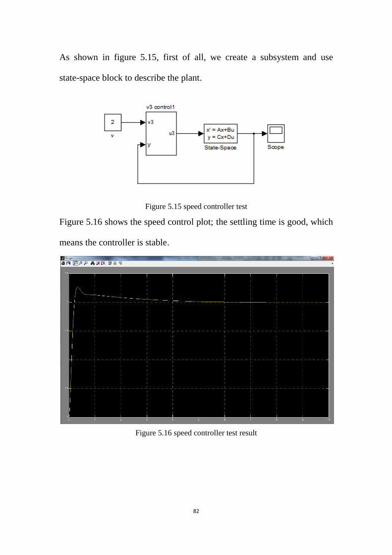
As shown in figure 5.15, first of all, we create a subsystem and use
state-space block to describe the plant.
Figure 5.15 speed controller test
Figure 5.16 shows the speed control plot; the settling time is good, which
means the controller is stable.
Figure 5.16 speed controller test result
83
5.4 Putting the whole system together
5.4.1 Kelvin-Voigt model
Kelvin-Voigt model is the basic model we use, and the whole plant could
be described in state-space blocks. We set:
0 0 10 0
0 0 0 10
3.315 3.315 0.5882 0.5882
3.315 3.315 0.5882 0.5882
A
,
0 0
0 0
8.533 0
0 8.533
B
Also we need to couple the control signal together, so set:
1 0.5 0.5
0.5 0.5uT
Matrixes A and B are used in state-space block to describe the
plant in Simulink. And matrix 1
uT
is used in gain block to decouple the
control signal.
Actually, there will be noise in the real experiment, so we use white noise
block to simulate noise. Finally the whole system could be organized as
shown in figure 5.17.

84
Figure 5.17 Kelvin-Voigt model test
There are two filters in the system to weaken the noise effect. According
to the system matrix given by Equation (4.19), the output is position and
tension, if we want to control speed, we also need get derivative of
position, so the filter1 is a combination of filter and derivative.
When we run the simulation, we get the plots shown in figures 5.18 and
5.19, the yellow line is speed, and the purple line is tension, we could see
the filter works obviously in the system.
According to the plots, the filter reduce the effect of noise, but it also
slow down the whole system, so we need to choose a suitable filter
depending on our need.

85
Figure 5.18 test result without filter
Figure 5.19 test result with filter
5.4.2 Three-parameter Maxwell model
Since in the three-parameter Maxwell model, the force is changing with
time, so it is difficult to apply state-space to describe the plant. To
organize the plant correctly, add a derivative block and a gain to build a
closed loop feedback. In this way, we could describe the tension.

86
In this model, desired velocity is 3 m/s, desired tension is 1 N. The
tension and velocity should become stable as quickly as possible. Figure
5.20 shows Maxwell model.
Figure 5.20 Maxwell model test
Before simulation, we need to set simulation time to 10 sec. And in the
configuration parameters option, set Type as “Fixed-step”, Fixed-step size
as 1e-3. This will speed up the simulation. We run the simulation to
generate figure 5.21:

87
Figure 5.21 test result without noise
Since the plant is quite complex, create a subsystem of Maxwell model to
simplify this plant. Select the plant blocks; add one input block, named
“current”; add one output block, and add the tension and velocity outputs
together. In this way, the whole system changes to figure 5.22:
Figure 5.22 subsystem of Maxwell model
Also, by noticing that, in the real experiment, there should be noise
existing. So we add white noise block to the plant:

88
Figure 5.23 Maxwell model with noise
Set noise power as 0.00001 and simulation time as 10 seconds. Run the
simulation, we obtain figure 5.24.
Figure 5.24 test result with noise
According to the plot, the max tension is almost 12 N. Although the
system is stable, the plot is bad; we need to choose another group of
parameters’ values in the controllers to make a better plot.

89
5.4.3Dzierzek model
Since in the Dzierzek model, there are several forces, such as Fm1 and Fm2,
changing with time, it is more difficult to apply state-space to describe
the plant. To organize the plant correctly, we add derivative blocks and
corresponding gains to build closed loop feedbacks. In this way, we could
describe the whole system.
The desired velocity is 5 m/s, desired tension is 2 N. The final goal is to
keep velocity and tension constant and stable. Figure 5.25 shows the
model.
Figure 5.25 Dzierzek model
A complex plant will always affect us to modify or improve the system.
Again select all the plant, add the outputs together, add input and output
blocks, and create the subsystem, as shown in figure 5.26.

90
Figure 5.26 Dzierzek subsystem model
The whole system is simplified. Next step, we add white noise block to
the system, the noise power is 0.00001, as shown in figure 5.27.
Figure 5.27 Dzierzek system with noise
Before simulation, we need to set simulation time as 10 sec. And in the
configure ration parameters option, set Type as “Fixed-step”, Fixed-step
size as 1e-3. This will speed up the simulation. When we run the
simulation, we will get figure 5.28:

91
Figure 5.28 Dzierzek system test result
The noise makes the plot unclear. To get a better plot, we add two filters
into the system. Since the output is position, the filter for velocity should
also include the derivative function, as shown in figure 5.29.
Figure 5.29 Dzierzek system with filters

92
Figure 5.30 test result
The noise effect is obviously reduced, but the filter also effects the
settling time and vibration of plot, as shown in figure 5.30.
To make this model more close to real conditions, we add a Viscous
Friction block to the tension output, as shown in figure 5.31. Exclude the
effect of noise at first.
Figure 5.31 Dzierzek with friction block

93
Figure 5.32 test result
Compared with the former result, there is obvious that the plot is changed,
as shown in figure 5.32.
Next step, add the noise and filters. We Notice that the filters may cause
the system to become unstable. So we need to consider both response
time and stability at the same time, as shown in figure 5.33.
Figure 5.33 Dzierzek with noise and friction blocks
Set the parameters in Viscous Friction block, suppose the coulomb
friction value is 1N, and coefficient of viscous friction is 0.5. Still add the

94
noise, filters and run the simulation to generate plot shown in figure 5.34.
Figure 5.34 test result
5.5 Analysis of result
5.5.1 Effects of poles’ locations
According to the plot of Maxwell model and Celvin-Vigot model, when
the simulation began, there are lots of damping in tension curves, which
means the tension estimator could not keep up with the output.
So suppose the estimator is too slow to changing with output.
Considering the parameters effects estimator are bet4, bet5 and bet6, it is
necessary to choose better poles’ locations. The original poles’ locations
are:
( 10,0),( 10,0),( 10,0)
The poles do not have a good damping ability, so we choose new poles:

95
( 60,0),( 50 15 ,0),( 50 15 ,0)i i
Calculating with Matlab, we got the equation:
3 2160 8725 163500 0s s s
So the corresponding parameters’ values are:
4
5
6
160
8725
163500
bet
bet
bet
When we run the simulation to test the result, we can see the result clearly,
excluding the effect of noise at first, as shown in figure 5.35 and 5.36.
Figure 5.35 Maxwell model test result

96
Figure 5.36 Dzierzek model test result
It is clear that the damping at beginning still looks bad. So suppose
another group of poles:
( 10,0),( 1 ,0),( 1 ,0)i i
With the help of Matlab, we get the equation:
3 212 22 20 0s s s
So the corresponding parameters’ values are: 4
5
6
12
22
20
bet
bet
bet
We run the simulation

97
Figure 5.37 Dzierzek model test result
Figure 5.37 shows the damping at beginning was reduced obviously, but
the settling time is longer. Since the dominate poles are ( 1 ,0),( 1 ,0)i i ,
so this result reflects the effects of poles’ locations.
Figure 5.38 Maxwell model test result
Figure 5.38 shows the damping part is also reduced. And there is a little
98
delay in settling time. This result shows that the dominate pole’s location
effect both settling time and damping ability of the system. And a better
response time often means a bad effect on damping ability.
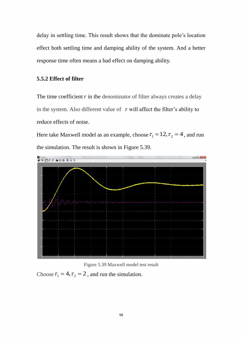
5.5.2 Effect of filter
The time coefficient in the denominator of filter always creates a delay
in the system. Also different value of will affect the filter’s ability to
reduce effects of noise.
Here take Maxwell model as an example, choose 1 212, 4 , and run
the simulation. The result is shown in Figure 5.39.
Figure 5.39 Maxwell model test result
Choose 1 24, 2 , and run the simulation.

99
Figure 5.40 Maxwell model test result
Compare the two results shown in figure 5.39 and 5.40, we could see the
settling time is much reduced, but the plots of velocity become very
rough. So the time coefficient is chosen by the priority between settling
time and noise reducing.
100
Reference
[1] Li Ting, Du Chunling, “The development status of the belt conveyor
drive systems”. Science, Vol. 3. 2007
[2] Chen Geng, Wen Lisheng, “New Progress of the friction drive
components”, machine design and research, vol.6,1985
[3] Li Yusheng, “Flat belt drive reliability”. Machinery Design &
Manufacture. Vol. 3, 1992.
[4] Cao Zhujia, “Flat belt drive design”. China Petroleum Machinery. Vol.
19, 1991.
[5] XU Lin, “The Virtual Assembly and Motion Simulation of
Machine-table Vice Basing on Solidworks”. Equipment Manufacturing
Technology, Sep, 2006.
[6] Wang Jizhong, “FEA model of tire structure”, Tire Industry, Vol. 22,
Pages 202-204, 2002.
[7] Zhiqiang Gao. “Active Disturbance Rejection Control: A Paradigm
Shift in Feedback Control System Design”, Proceedings of the 2006
American Control Conference. Minneapolis, Minnesota, USA, June
14-16, 2006.
[8] J. Han, “Nonlinear PID controller”, J.Autom. vol.20, no.4,
pages.487-490, 1994.
[9] Yoshikazu Nishikawa, Nobuo Sannomiya, Tokuji Ohta, Haruki

101
Tanaka,” A method for auto-tuning of PID control parameters”.
Automatica, Vol. 20, Issue 3, May 1984, Pages 321-332
[10] JINGQING HAN. “From PID to Active Disturbance Rejection
Control”. IEEE transactions on industrial electronics, VOL. 56, NO. 3,
MARCH 2009.
[11] K. J. Astrom and T. Hagglund, “PID Control,” The Control
Handbook, W.S. Levine, Ed. page 198, CRC Press, 1996.
[12] Z. Gao and R. Rhinehart, “Theory vs. Practice Forum,” Proc. of the
2004 American Control Conference, June 30-July 2, 2004, Boston MA,
pages 1341-1349.
[13] J. Han, “Control Theory: Is it a Theory of Model or Control?”
Systems Science and Mathematical Sciences, Vol.9, No.4, pages 328-335.
1989.
[14] Jingqing Han. “Auto Disturbance Rejection Control Technique”.
Frontier Science, Vol. 1. NO.1, January 2007.
[15] Farhad Tabaddor, “Rubber elasticity models for finite element
analysis”. Uniroyal Goodrich, Akron, OH 44318, U.S.A.
[16] SHASKA K. “The characterization of nonlinear viscoelastic
isolators”. [D]. Michigan:Wayne State University, 2005.
[17] Gent A N. Engineering with rubber [M]. 2nd.Beijing:Chemical
Industry Press, 2002
[18] DZIERZEK S. “Experiment-based modeling of cylindrical rubber

102
bushings for the simulation of wheel suspension dynamic behavior” [R].
SAE 2000-01-0095, 2000.
[19] Ping Jiang, Ping Jiang ; Jing-Yu Hao, Jing Yuhao, Xiao-Ping Zong,
Xiao Pingzong; Pei Guangwang, Pei Guang Wang. “Machine Learning
and Cybernetics”, July 2010, Vol.2, pages.927-931
[20] Jiang Ping, Jiang Ping; Bingshu Wang, Bingshu Wang. “Information
and Computing”, June 2010, Vol.2, pages.151-154