modeling and calculation of electromagnetic ﬁeld in the

Turk J Elec Eng & Comp Sci, Vol.17, No.3, 2009, c© TUBITAK

doi:10.3906/elk-0908-182

Modeling and calculation of electromagnetic field in the

surroundings of a large power transformer

Leonardo STRAC1, Franjo KELEMEN2, Damir ZARKO3

1Koncar Power Transformers Ltd., Research and Development DepartmentJosipa Mokrovica 6, 10090 Zagreb-CROATIA

e-mail: [email protected] Power Transformers Ltd., Research and Development Department

Josipa Mokrovica 6, 10090 Zagreb-CROATIAe-mail: [email protected]

3University of Zagreb, Faculty of Electrical Engineering and Computing,Department of Electrical Machines, Drives and Automation Unska 3, 10000 Zagreb-CROATIA

e-mail: [email protected]

Abstract

The presented study compares measured and calculated electromagnetic field quantities in the surroundings

of a large power transformer with the aim to avoid the necessity of measuring the field on subsequent units

and use a computer model instead. The influences of various objects located in the vicinity of the transformer

during measurement are also analyzed and are taken into account in a computer model.

Key Words: Large power transformer, electromagnetic field, finite element method.

1. Introduction

Large power transformers produce electric and magnetic fields that can affect human health and have influence onthe environment. Therefore, most countries have legal regulations regarding peak values of electromagnetic fieldto which people in residential areas, offices or industrial plants may be exposed [1–3]. Although switchyardsare usually placed on isolated locations, customers who purchase power transformers often require technicaldocumentation and certificate about electromagnetic field emission of a transformer.

A background of this project was a special customer request for one transformer. The transformer wasto be placed in a switchyard near an office building. The customer requested peak electric field less than5 kV/m and peak magnetic field less than 100 μT at a distance of 30 m from the transformer (tank). The basictransformer ratings are: 3-phase transformer, 220 MVA, 240 kV, 50 Hz. Due to lack of experience regardingsimilar problems, the most reasonable course of action was to find a similar transformer (by the criteria of

nominal power, nominal voltage level and short circuit voltage) in the current factory production and makeinitial tests. A similar transformer with basic ratings 3-phase transformer, 250 MVA, 300 kV, 50 Hz was chosen.

301

Turk J Elec Eng & Comp Sci, Vol.17, No.3, 2009

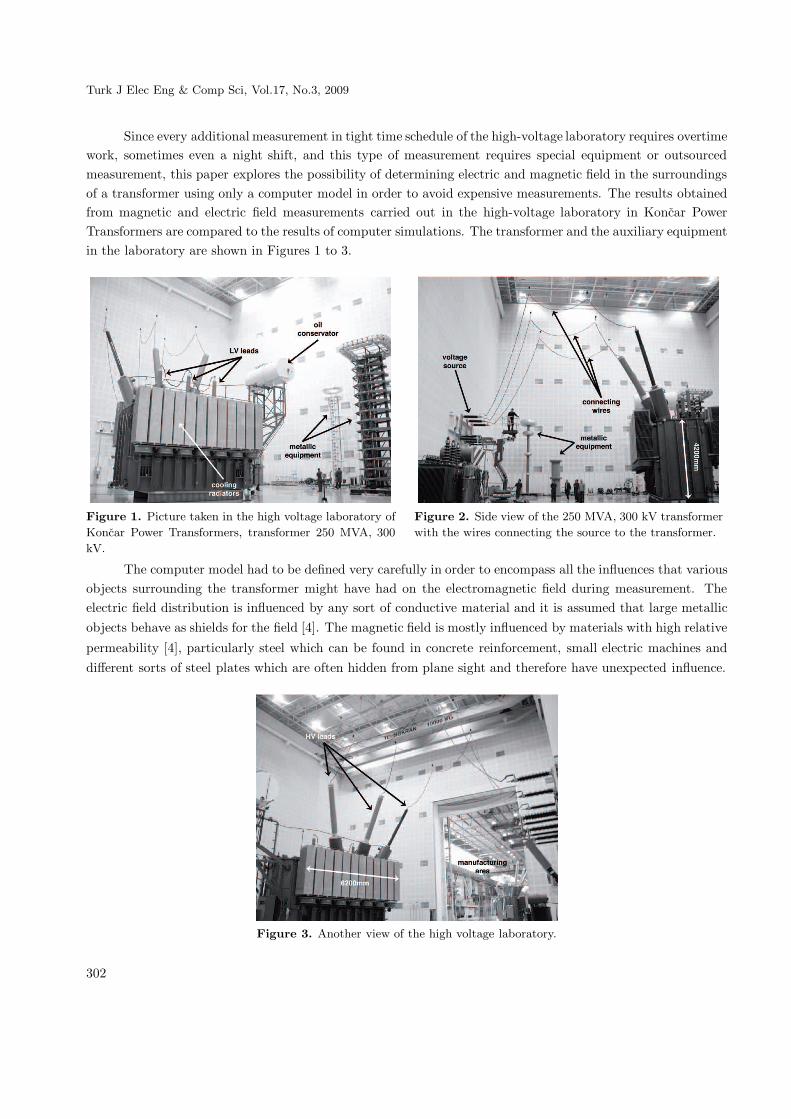
Since every additional measurement in tight time schedule of the high-voltage laboratory requires overtimework, sometimes even a night shift, and this type of measurement requires special equipment or outsourcedmeasurement, this paper explores the possibility of determining electric and magnetic field in the surroundingsof a transformer using only a computer model in order to avoid expensive measurements. The results obtainedfrom magnetic and electric field measurements carried out in the high-voltage laboratory in Koncar PowerTransformers are compared to the results of computer simulations. The transformer and the auxiliary equipmentin the laboratory are shown in Figures 1 to 3.

Figure 1. Picture taken in the high voltage laboratory of

Koncar Power Transformers, transformer 250 MVA, 300

kV.

Figure 2. Side view of the 250 MVA, 300 kV transformer

with the wires connecting the source to the transformer.

The computer model had to be defined very carefully in order to encompass all the influences that variousobjects surrounding the transformer might have had on the electromagnetic field during measurement. Theelectric field distribution is influenced by any sort of conductive material and it is assumed that large metallicobjects behave as shields for the field [4]. The magnetic field is mostly influenced by materials with high relative

permeability [4], particularly steel which can be found in concrete reinforcement, small electric machines anddifferent sorts of steel plates which are often hidden from plane sight and therefore have unexpected influence.

Figure 3. Another view of the high voltage laboratory.

302

L. STRAC, F. KELEMEN, D. ZARKO: Modeling and calculation of electromagnetic field...,

The measurement is managed by Koncar Institute for Electrical Engineering, Zagreb, with a PMM EHP-50C Electric and Magnetic Field Analyzer and a PMM 8053 Field Meter. Technical specifications of EHP-50CAnalyzer are: frequency range 5 Hz – 100 kHz for electric and magnetic field, sensitivity 0.01 V/m, 1 nT,

absolute error ± 0.5 dB (@ 50 Hz and 1 kV/m) (@ 50 Hz and 0.1 mT), electric and magnetic field rejection>20 dB. Measured values are average of x,y, and z components for the frequency of 50 Hz. A wooden tripodwas used to hold a probe in front of the transformer. The electromagnetic field is calculated using 3D finiteelement software Ansoft Maxwell, a standard FEM software used in Koncar Power Transformers. Magnitude

of field values were calculated using the equation F =√

F 2x + F 2

y + F 2z .

2. Model of the 250 MVA, 300 kV transformer

All finite-element models in this paper are made using Ansoft Maxwell commercial software. Magnetic fieldwas calculated in magnetostatic mode. Since there are no induced currents in this type of calculation, theconductivity of all materials is set to zero (except for copper wires). The material for the surrounding box of

the transformer model is vacuum. The parts made of transformer steel (core and tank shields) have hundred

times higher relative permeability than those made of plain steel (tank, clamping plates and consoles). Thecurrent sources are used in the model and copper conductors are simulated to be stranded in order to ensureuniformly distributed current across the conductor’s cross section. The boundary conditions at the end regionare set as Neumann boundaries. All parts inside the tank were modeled as simple as possible in order to reducethe computational time without significantly affecting the overall field solution. The model mesh containsabout one million tetrahedrons in the final mesh refinement, and it takes about 12 hours of computing time ona multi-core workstation to complete the calculation.

The model for calculating electric field is very similar. In this case voltage sources were used for thetransformer leads.

The basic model is established for the autotransformer of nominal power of 250 MVA and a nominalvoltage of 300 kV. All the calculations are carried out for the frequency of 50 Hz because it is the transformer’snominal frequency. Since this is not a special purpose transformer (rectifying, HVDC, etc.), it was not necessaryto calculate and measure electromagnetic field at higher frequencies. This computer model is valid for thefrequency of 60 Hz as well. The initial assumption was that it should be enough to model an empty tank andshort circuited low-voltage (LV) and high-voltage (HV) leads excited with the nominal currents to calculatethe distribution of magnetic field in the space surrounding the transformer. However, results of the calculationdiffered from the measured values more than 20 dB, and the conclusion was that the model was not detailedenough. For that reason there were numerous improvements that had to be added to the model, like oilconservator, cooling radiators, wires connecting the source on the laboratory wall to the leads, laboratory’sFaraday cage and, finally, the transformer in the model was moved to the exact position and oriented adequatelyrelative to the laboratory walls. After these improvements have been made, the calculated field distributionnear the transformer was significantly closer to the measured one (up to the 10 dB difference), but the field 5

to 10 meters from the transformer was too small (10 to 19 dB difference for the HV and LV side).

As it can be seen in the Table 4, in the column Measured/Leads (calculated using equation

20 Log(Bmeasured /Bcalc Leads), the difference between the measured values and the values calculated for themodel with leads is increasing rapidly with distance. At this point it was obvious that the field originating

303


from the active part of the transformer cannot be ignored although the transformer tank is an excellent EMshield. In the end, three supplemental models have been derived from the basic model: the first to calculatestray magnetic field of the windings, the second to calculate magnetic field caused by the leads stray flux andthe third to calculate electric field caused by the leads.

The magnetic field calculation is separated in two different tasks because it would be very difficult tomake a detailed model incorporating both helix type winding and leads. The helix-shaped windings on allphases, including both high-voltage and middle-voltage windings, would form an extremely complex geometry.Hence, the finite element mesh for such a model would be too demanding for the available computer hardware.Moreover, the solution of magnetic field in the air surrounding the transformer would probably contain largeerrors because the software would have to deal predominantly with complex mesh inside the transformer. Forthat reason the first model has cylinder-shaped windings, closed tank without openings and does not have leads(Figures 4 to 5), while the second model does not incorporate windings, but only the short circuited leads

(Figure 6).

��

��

��

��

��

��

��

�

Figure 4. The model with windings for magnetic field

calculation, 250 MVA, 300 kV transformer.

Figure 5. Detail of the active part of the 250 MVA,

300 kV transformer.

The model for calculating electric field (Figure 7) is similar to the model without windings for magneticfield calculation. The main difference is that the leads are not short circuited. The influence of windings isneglected because the windings are well shielded by the earthed tank.

304


��

��

��

��

��

Figure 6. The model with leads for magnetic field calcu-

lation, 250 MVA, 300 kV transformer.

Figure 7. The model with leads for electric field calcula-

tion, 250 MVA, 300 kV transformer.

Since the laboratory is not an empty space and the transformer is quite a complex device, variousmodifications have to be made on the computer model in order to better describe the physical reality [5]. Thecopper lines that connect the transformer to the current source are particularly important. Both the electric andthe magnetic model (with leads) have to include copper lines which connect the leads and the source because oftheir great influence on the field distribution throughout the space. The oil conservator is included in all threemodels, but has the greatest impact on electric field calculation. The similar situation is with tank shields,which are made from transformer steel sheets and are located on the inner tank wall surface. They have thegreatest influence on magnetic field, but they are present in all three models. The influence of the iron Faradaycage that is built in the high voltage laboratory on both electric and magnetic field has been considerable, so ithad to be taken into account. The Faraday cage is modeled as a thin empty iron box that surrounds the entiremodel at the appropriate distance.

All the calculations were performed using Ansoft Maxwell finite element software in magnetostatic andelectrostatic calculation mode.

All the field measurements were carried out on the high voltage (HV) side, middle voltage (MV) side, low

voltage (LV) side and oil conservator (CS) side of the transformer (Figure 8). On each side the measurements

were carried out 1, 2, 4, 6, 8 and 10 meters away from the tank respectively (where that was possible) and at aheight of 1.25 meters from the bottom of the transformer.

Table 1 represents peak ampere-turns for high voltage (HV), middle voltage (MV) and regulation windingused in the model for magnetic field calculation with the winding and without leads. These are the ampere-turnsfor the neutral regulation position. Table 2 represents the peak current in the high voltage (HV), middle voltage

(MV) and low voltage (LV) leads used in the model for magnetic field calculation with the leads and without

winding. Table 3 gives the values of peak voltages applied to the high voltage (HV), middle voltage (MV) and

low voltage (LV) leads used in the model for electric field calculation.

305


��

��

��

��

Figure 8. Top view of the transformer with marked measurement points, 250 MVA, 300 kV transformer.

Table 1. Peak ampere-turn values in the windings for the magnetic field model with windings, 250 MVA, 300 kV

transformer.

Peak ampere-turnsHV MV regulation

Phase 1 182500 -202000 19500Phase 2 -365000 404000 -39000Phase 3 182500 -202000 19500

Table 2. Values of peak current in the leads for the magnetic field model with leads, 250 MVA, 300 kV transformer.

Peak current [A]HV MV LV

Phase 1 371 773 0Phase 2 -742 -1546 0Phase 3 371 773 0

Table 3. Values of peak voltage in the leads for the electric field model with leads, 250 MVA, 300 kV transformer.

Peak voltage [V]HV MV LV

Phase 1 336804 161666 -15556Phase 2 0 0 31112Phase 3 -336804 -161666 -15556

3. Results for the 250 MVA, 300 kV transformer

3.1. Magnetic field

The calculation of the magnetic field was carried out in two parts. In the first part, only the field from thewindings, and in the second part only the field from the leads was calculated at each measurement point. Later,the two values were added.

306


From Table 4 and Figures 9 to 10 it can be noticed that the differences between calculated and measuredvalues are not small in an absolute sense, but the calculated magnetic field in the model behaves qualitativelyas the measured one. It is also evident that the measured magnetic field does not diminish as fast as it couldbe expected, and this may be caused by conductors beneath the floor in the laboratory. Additionally, thepoint HV 08 has unusually high flux density because of the influence of the current source near the laboratorywall. Both effects could not have been reconstructed in the model. As the columns Measured/Leads and

Measured/Total in the Table 4 show, introducing the model of the active part was justified since the differencebetween measured and calculated values is reduced.

3.2. B. Electric field

The calculation of the electric field was more straightforward than the calculation of the magnetic field. Theinfluence of the winding and wires inside the tank was neglected, so only the field from the leads was taken intoaccount.

Table 4. Peak values of flux density in the surroundings of the 250 MVA, 300 kV transformer.

distance point Windings Leads Total Measured Me./Le. Me./Tot.[m] Br[uT] Br[uT] Br[uT] Bm[uT] [dB] [dB]1 HV 01 4,64 7,95 12,59 14,52 5,23 1,242 HV 02 2,90 5,54 8,44 9,76 4,92 1,264 HV 04 1,60 2,99 4,58 6,08 6,18 2,456 HV 06 1,61 1,59 3,20 5,57 10,90 4,818 HV 08 0,38 0,79 1,17 7,30 19,28 15,88

1 LV 01 1,25 10,16 11,41 8,71 -1,34 -2,352 LV 02 1,06 5,57 6,63 7,45 2,53 1,014 LV 04 0,58 2,66 3,24 5,33 6,04 4,336 LV 06 0,45 1,19 1,64 3,78 10,03 7,258 LV 08 0,25 0,75 1,00 2,81 11,44 8,9810 LV 10 0,16 0,42 0,58 2,03 13,64 10,84

1 MV 01 5,32 8,76 14,09 25,32 9,22 5,092 MV 02 3,37 6,66 10,03 17,08 8,18 4,624 MV 04 0,98 3,04 4,02 8,2 8,63 6,196 MV 06 0,14 1,38 1,52 4,62 10,48 9,648 MV 08 0,11 1,01 1,12 2,66 8,44 7,5310 MV 10 0,09 0,69 0,78 1,56 7,12 6,07

1 CZ 01 1,33 7,18 8,51 5,44 -2,41 -3,892 CZ 02 0,80 3,88 4,68 4,5 1,29 -0,334 CZ 04 0,44 2,50 2,94 3,19 2,11 0,706 CZ 06 0,24 1,29 1,54 2,25 4,81 3,318 CZ 08 0,09 0,58 0,67 1,63 9,02 7,76

The distribution and the values of the electric field in the model, shown in Table 5 and Figures 11 to 12,are in a reasonably good agreement with measurements (difference is up to 12 dB with tendency of decreasing

with distance), with the exception of the LV side. The reason why the measured electric field on the LV side is

307


much smaller than calculated in the model remains unclear, but the reason probably lies in different layout ofthe copper lines in the model and the actual transformer.

��

�

�

��

��

��

��

�

�� !��"��#��$��%��&�'

(&)'

��*��*�� *��*��

��*��*�� *��*��

μ

Calculated and measured values of magnetic induction

0

5

10

15

20

25

30

1 2 3 4 5 6 7 8 9 10distance[m]

B[

T]

MV_tot_calc CS_tot_calc

MV_tot_meas CS_tot_meas

μ

Figure 9. Calculated and measured values of flux density

in the surroundings of the 250 MVA, 300 kV transformer,

part 1.

Figure 10. Calculated and measured values of flux den-

sity in the surroundings of the 250 MVA, 300 kV trans-

former, part 2.

Table 5. Peak values of electric field outside the 250 MVA, 300 kV transformer.

distance point Leads Measured Me./Le.[m] Er [V/m] Em [V/m] [dB]1 HV 01 71 96 2,542 HV 02 107 177 4,374 HV 04 214 273 2,146 HV 06 170 253 3,448 HV 08 111 180 4,1910 HV 10 57 111 5,80

1 LV 01 852 276 -9,782 LV 02 960 331 -9,264 LV 04 1054 301 -10,876 LV 06 792 241 -10,338 LV 08 443 350 -2,05

1 MV 01 32 22 -3,312 MV 02 120 37 -10,194 MV 04 120 61 -5,906 MV 06 99 61 -4,298 MV 08 45 47 0,3910 MV 10 24 35 3,39

1 CZ 01 200 55 -11,262 CZ 02 228 60 -11,654 CZ 04 209 71 -9,366 CZ 06 161 62 -8,288 CZ 08 121 45 -8,60

308


��

�� !��"��#��$��%��

�� !��"��#��$��%��&�'

+&�

,�'

��*�� *��*�� *��

��

�� !��"��#��$��%��

�� !��"��#��$��%��&�'

+&�

,�'

��*��-*��

��*��-*��

Figure 11. Calculated and measured values of electric

field outside of 250 MVA, 300 kV transformer, part 1.

Figure 12. Calculated and measured values of electric

field outside of 250 MVA, 300 kV transformer, part 2.

4. Results for the 220 MVA, 240 KV transformer

After acquiring experience with the model of the 250 MVA, 300 kV transformer, the transformer for which thecustomer originally requested specific electromagnetic field emission was modeled in the same manner. Althoughthese two transformers are considered similar from the manufacturing point of view, they differ in many waysthat can impact the distribution of electromagnetic field: nominal power and voltage, short circuit voltage,layout of the winding, position of the leads, number, position and size of the cooling radiators, size of the oilconservator etc. (Figure 13).

Figure 13. The model with leads for electric field calculation, 220 MVA, 240 kV transformer.

309


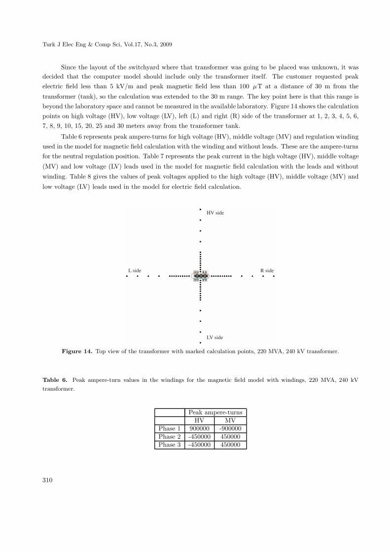
Since the layout of the switchyard where that transformer was going to be placed was unknown, it wasdecided that the computer model should include only the transformer itself. The customer requested peakelectric field less than 5 kV/m and peak magnetic field less than 100 μT at a distance of 30 m from the

transformer (tank), so the calculation was extended to the 30 m range. The key point here is that this range isbeyond the laboratory space and cannot be measured in the available laboratory. Figure 14 shows the calculationpoints on high voltage (HV), low voltage (LV), left (L) and right (R) side of the transformer at 1, 2, 3, 4, 5, 6,7, 8, 9, 10, 15, 20, 25 and 30 meters away from the transformer tank.

Table 6 represents peak ampere-turns for high voltage (HV), middle voltage (MV) and regulation windingused in the model for magnetic field calculation with the winding and without leads. These are the ampere-turnsfor the neutral regulation position. Table 7 represents the peak current in the high voltage (HV), middle voltage

(MV) and low voltage (LV) leads used in the model for magnetic field calculation with the leads and without

winding. Table 8 gives the values of peak voltages applied to the high voltage (HV), middle voltage (MV) and

low voltage (LV) leads used in the model for electric field calculation.

��

��

�� .��

Figure 14. Top view of the transformer with marked calculation points, 220 MVA, 240 kV transformer.

Table 6. Peak ampere-turn values in the windings for the magnetic field model with windings, 220 MVA, 240 kV

transformer.

Peak ampere-turnsHV MV

Phase 1 900000 -900000Phase 2 -450000 450000Phase 3 -450000 450000

310


Table 7. Values of peak current in the leads for the magnetic field model with leads, 220 MVA, 240 kV transformer.

Peak current [A]HV MV

Phase 1 764 2700Phase 2 -382 -1350Phase 3 -382 -1350

Table 8. Values of peak voltage in the leads for the electric field model with leads, 220 MVA, 240 kV transformer.

Peak voltage [V]HV MV

Phase 1 339411 96167Phase 2 -169706 -48083Phase 3 -169706 -48083

4.1. Magnetic field

Table 9. Peak values of calculated flux density in the surroundings of the 220 MVA, 240 kV transformer, part 1.

distance point Windings Leads Total[m] Bcalc[μT] Bcalc[μT] Bcalc[μT]1 HV 01 35,05 37,46 72,522 HV 02 17,99 38,40 56,393 HV 03 7,63 27,72 35,354 HV 04 4,69 19,69 24,385 HV 05 2,60 13,44 16,046 HV 06 2,13 9,88 12,017 HV 07 1,26 7,21 8,478 HV 08 0,89 5,53 6,429 HV 09 0,68 4,16 4,8410 HV 10 0,47 3,33 3,8015 HV 15 0,17 1,22 1,3920 HV 20 0,08 0,52 0,6025 HV 25 0,04 0,28 0,3330 HV 30 0,03 0,15 0,18

1 R 01 11,06 26,68 37,742 R 02 5,88 14,87 20,753 R 03 3,03 9,09 12,124 R 04 2,25 5,83 8,085 R 05 1,53 3,98 5,506 R 06 0,83 2,62 3,457 R 07 0,62 2,10 2,728 R 08 0,54 1,59 2,139 R 09 0,46 1,29 1,7610 R 10 0,39 1,04 1,4215 R 15 0,08 0,42 0,5120 R 20 0,06 0,23 0,2925 R 25 0,04 0,11 0,1530 R 30 0,02 0,08 0,11

311


Table 10. Peak values of calculated flux density in the surroundings of the 220 MVA, 240 kV transformer, part 2.

distance point Windings Leads Total[m] Bcalc[μT] Bcalc[μT] Bcalc[μT]1 LV 01 33,32 63,86 97,172 LV 02 16,63 53,50 70,133 LV 03 8,13 36,05 44,184 LV 04 3,81 23,84 27,665 LV 05 2,75 16,80 19,556 LV 06 1,50 11,66 13,167 LV 07 1,20 8,17 9,378 LV 08 0,94 6,19 7,139 LV 09 0,73 4,69 5,4210 LV 10 0,52 3,70 4,2215 LV 15 0,16 1,29 1,4520 LV 20 0,10 0,52 0,6225 LV 25 0,04 0,29 0,3330 LV 30 0,04 0,15 0,18

1 L 01 9,99 19,98 29,972 L 02 6,72 11,42 18,133 L 03 3,59 6,74 10,334 L 04 0,61 4,56 5,175 L 05 1,16 3,14 4,306 L 06 0,99 2,42 3,417 L 07 0,84 1,86 2,708 L 08 0,60 1,48 2,089 L 09 0,47 1,22 1,6910 L 10 0,36 0,99 1,3515 L 15 0,12 0,36 0,4820 L 20 0,05 0,21 0,2625 L 25 0,04 0,12 0,1630 L 30 0,03 0,09 0,11

)��

�

��

!�

"�

$�

��

�� &�'

(&

)'

��

.��

��

��

μ

Figure 15. Calculated values of flux density in the surroundings of the 220 MVA, 240 kV transformer.

312


4.2. Electric field

Table 11. Peak values of calculated electric field outside the 220 MVA, 240kV transformer.

distance point Leads distance point Leads[m] E[V/m] [m] E[V/m]1 HV 01 1691 1 LV 01 15192 HV 02 2547 2 LV 02 24923 HV 03 1989 3 LV 03 18444 HV 04 1575 4 LV 04 13645 HV 05 1278 5 LV 05 9676 HV 06 796 6 LV 06 6997 HV 07 559 7 LV 07 6148 HV 08 437 8 LV 08 3969 HV 09 337 9 LV 09 39410 HV 10 275 10 LV 10 24015 HV 15 112 15 LV 15 10220 HV 20 58 20 LV 20 5025 HV 25 31 25 LV 25 2630 HV 30 25 30 LV 30 36

1 R 01 3843 1 L 01 23152 R 02 2221 2 L 02 14383 R 03 1347 3 L 03 10764 R 04 885 4 L 04 7865 R 05 612 5 L 05 5596 R 06 536 6 L 06 4727 R 07 356 7 L 07 3798 R 08 286 8 L 08 2899 R 09 223 9 L 09 20310 R 10 183 10 L 10 18315 R 15 78 15 L 15 7920 R 20 41 20 L 20 4025 R 25 23 25 L 25 2030 R 30 15 30 L 30 13

��

�

��

��

��

!��

��

�� &�'

+&�

,�'

�� .��

��

Figure 16. Calculated values of electric field outside of 220 MVA, 240 kV transformer.

313


As it can be seen from Tables 9 to 11 and Figures 15 to 16 the peak values of electric and magnetic arebelow the customer request of 5 kV/m and 100 μT respectively, not only at 30 m from the transformer, butacross the whole range. It can also be noticed that the results are quite different in the close surrounding of thetransformer compared to the previous case. The reasons for that difference lie in a different geometry of the twotransformers: different amount of winding stray flux, lower position of the leads, and most importantly, there is adifferent layout of the cooling radiators which act as a shield to electromagnetic field. The 250 MVA transformerhas the cooling radiators across the entire tank in both HV and MV sides, while 220 MVA transformer missescouple of radiators in the middle, just in the line with the calculation points on the HV and LV side. Therefore,the 220 MVA transformer does not have an electromagnetic shield in the form of cooling radiators resulting inhigher field values in the first 5 meters from the transformer.

5. Conclusion

The presented analysis deals with the comparison of measured and calculated magnetic and electric field in thesurroundings of a power transformer.

Although it is possible to calculate the field using a 3D finite-element model, the main difficulty is to getprecise absolute values of magnetic flux density and electric field strength that can be confirmed by measurement.The relative difference between the measured and the calculated values in this case can be as large as 15 dB. Thepeak values of the flux density in the surrounding area of the transformer are typically below 25 μT, and thoseof the electric field below 500 V/m, which are both values that can be easily disturbed by parasitic influencesin both the model and the actual environment, so the results shown in this paper can be considered acceptable.

It can also be noticed that objects in the transformer’s surroundings have great impact on the magneticand electric field distribution in the vicinity of the transformer. The values of electromagnetic field measuredon site can differ significantly from those measured in the laboratory, so it can be concluded that the field in thesurroundings of the transformer on site cannot be predicted reliably by measuring the field in the laboratoryconditions. That applies to the model as well. For quantitative accuracy all parasitic influences must be knownin advance, which is very difficult to achieve.

Computer modeling can be very useful to model just the transformer in an empty space. In that mannerthe influence of the transformer itself can be more easily distinguished from the influences of other sources offield once the transformer is on site.

References

[1] European Council Recommendation of 12 July 1999. on the limitation on exposure of the general public to

electromagnetic fields (0 Hz to 300 GHz), 1999/519/EC.

[2] International Commission on Non-Ionizing Radiation Protection, Guidelines for Limiting Exposure to Time-Variant

Electric, Magnetic and Electromagnetic Fields (up to 300 GHz), Health Phys.,Vol. 74, 4, (1998) 494-522.

[3] Zakon o zastiti od neionizacijskog zraenja, Narodne novine 105/99, Croatia 1999.

[4] Z. Haznadar, Z. Stih: Electromagnetic Fields, Waves and Numerical Methods, IOS - Press, Amsterdam, Berlin,

Oxford, Tokyo, Washington, 2000.

[5] O. Hartal, M. Merzer: Magnetic shielding of power plants in large facilities, 2003. IEEE International Symposium

on Electromagnetic Compatibility, pages 966 - 970 Vol. 2.

314

modeling and calculation of electromagnetic ﬁeld in the

Documents