modeling and control approach for a complex-shaped

American Journal of Mechanical Engineering, 2019, Vol. 7, No. 4, 158-171 Available online at http://pubs.sciepub.com/ajme/7/4/2 Published by Science and Education Publishing DOI:10.12691/ajme-7-4-2

Modeling and Control Approach for a Complex-Shaped Underwater Vehicle

G.A.C.T. Bandara*, D.A.A.C. Ratnaweera, D.H.S. Maithripala

Department of Mechanical Engineering, University of Peradeniya, KY 20400, Sri Lanka *Corresponding author: [email protected]

Received August 19, 2019; Revised September 26, 2019; Accepted October 16, 2019

Abstract This paper presents the trajectory tracking and the path planning algorithm based on an adaptive control law to operate a complex-shaped low speed autonomous underwater vehicle (AUV) in a challenging environment of non-linearity, time variance and unpredictable external disturbances. Firstly, computational fluid dynamic (CFD) simulations are used to compute the added mass matrix and the damping matrix. Secondly, the adaptive controller is implemented to track the desired trajectory. This desired state-dependent regressor matrix-based controller provides consistent results even under hydrodynamic parametric uncertainties. The stability of the developed controller is verified using Lyapunov’s direct approach. Moreover, the proposed control law adopts quaternions to represent the attitude errors and thus avoids the representation of singularities that occur when using the Euler angle description of the orientation. Thirdly, an efficient underwater path planning algorithm is developed based on vehicle-fixed-frame error variables. The simulations are done to compute the optimal path of the AUV which minimizes the travelling time. Finally, an optimal thrust allocation for the desired values of forces and moments acting on the vehicle is found via a model-based unconstrained thrust allocation. The results show that the AUV asymptotically converges on the desired trajectory and the path with a minimum time. At this moment, the propulsion forces approach zero, which further assures the accuracy of the controller. Hence, the effectiveness and the robustness of the developed algorithm are acceptable to design the AUV.

Keywords: autonomous underwater vehicle (AUV), CFD modelling, adaptive control, trajectory, path planning, optimal thrust allocation

Cite This Article: G.A.C.T. Bandara, D.A.A.C. Ratnaweera, and D.H.S. Maithripala, “Modeling and Control Approach for a Complex-Shaped Underwater Vehicle.” American Journal of Mechanical Engineering, vol. 7, no. 4 (2019): 158-171. doi: 10.12691/ajme-7-4-2.

1. Introduction

Over last two decades, autonomous underwater vehicles (AUVs) have played major roles in underwater applications, and have a large variety of types and shapes. Especially small size, complex-shaped AUVs have more flexibility to reach the areas where remote operating vehicles (ROVs) and human occupied vehicles (HOVs) cannot be deployed. AUVs can also be operated in risky and hazardous environments. Meanwhile, complex-shaped AUVs have more DOFs than conventional torpedo-shaped AUVs to increase the maneuverability in complex underwater spaces.

There are three key factors to be considered in the motion control of an AUV: First, an accurate hydrodynamic model, second, an advanced control system, and third, an optimum thrust allocation. Yamamoto revealed in [1] that a model-based control system is more effective in case of dynamics of the AUV is known to some extent. Furthermore, an empirical model generally fails to represent the dynamics of the AUV over a wide operating region that was noticed by Ferreira [2]. Thus, to

get an accurate hydrodynamic model of the complex-shaped AUVs is vital to design a controller. In addition to that, it is an arduous task to build a suitable controller for an AUV due to the complexity of hydrodynamic parameters containing highly non-linear and coupled terms. Moreover, the literature in the field of the optimum thrust allocation is little to be known [3]. Particularly, the importance of the optimization of the thrust forces of AUVs has been disregarded so far.

Scaled and full-scaled experiment, empirical formula, and computational approach are the existing methods to model the underwater vehicles. The scaled and full-scaled experiments are the most expensive methods because these ones require costly devices like towing tanks, but provide accurate hydrodynamic parameters. References [4,5] provide the methods to do the experiments without the towing tank. Furthermore, the empirical formulas usually give the acceptable results on the underwater vehicles that have slender bodies such as torpedo-shaped AUVs as noticed in [6]. Lastly, computation approaches are the best way to find the hydrodynamic parameters under low cost. Nevertheless, vast knowledge and experience are the prime factors to model the complex-shaped AUVs. Potential and finite element theory-based software such as

American Journal of Mechanical Engineering 159

ANSYS FLUENTTM, ANSYS AQWATM, ANSYS CFXTM, and WAMITTM is used in this method. WAMITTM overcomes the other software to compute the added mass matrix [7]. Similarly, ANSYS CFXTM leads the case of finding damping matrix [8].

There are so many control systems proposed to the track trajectories and to plan the desired path for AUVs. The horizontal tracking control for the AUVs based on a non-linear sliding mode incremental feedback model was introduced in [9] to track the desired trajectories. The error dynamics on the horizontal plane were proposed in [10] to plan and track the trajectories using the closed loop tracking controller and the backstepping method was used to stabilize the system. To track the given trajectories in the presence of ocean currents, a feedback controller was introduced in [11] using ling of sight (LOS), and a sliding mode controller based on both LOS and cross track error approach was presented in [12]. The trajectory planning for the AUVs was addressed in [13] to provide ocean processes of the real-time ocean model. The wheel robot was controlled to track the desired trajectories in [14] using a linearized fuzzy adaptive controller with the backstepping feedback. The trajectory tracking of the AUVs was implemented using the adaptive tracking controller based on a radial basis function neural network (RBF-NN) [15]. A dynamic surface control (DSC) and minimal learning parameters (MLP) based on a robust adaptive neural network tracking control for the underwater vehicle have been used in [16]. The learning method of a neural network has been used to model the stability and robustness adaptive controller for a nonholonomic robot [17]. In [18,19], they have described the path planning method based on a velocity field using the starting point and the desired ending point within a minimum time period. The coordinate path followed by underactuated AUVs was outlined, based on the convergence of geometric errors with respect to the origin of the vehicle that coincides with the center of gravity [20]. The path tracking based on the marching algorithm has been used in [21] for the path planning on a fixed depth. The combined path following and trajectory tracking for the AUVs have been discussed in [22] using the backstepping method, where Lyapunov’s direct approach was used to develop the kinematic of the AUVs. The optimal path planning for the AUVs in fast flowing, complex fluid flow was proposed using the methods of cost function, parametrization, and principle of minimum energy [19].

Recommended techniques of finding the hydrodynamic, trajectory tracking and path planning methods for AUVs have been noted in literature. However, an uncertainty of their hydrodynamic parameters, including non-linear hydrodynamic effects, parameter variations, and ocean current disturbance, causes difficulties when designing the suitable controllers. To overcome these problems, there should be a controller that could be operated under the well-defined hydrodynamic model.

In our work, the complex-shaped AUV that was used for the simulations is shown in Figure 1. The placement of 6 thrusters is only considered in Section 5. Furthermore, the configuration details of the AUV are listed in Table 1.

Figure 1. 3D CAD images of the AUV [23]

Table 1. Characteristics of the complex-shaped AUV

Size (L) 0.525 𝑚𝑚, (W) 0.406 𝑚𝑚, (H) 0.395 𝑚𝑚 Weight in air 16.00 𝑘𝑘𝑘𝑘 Propulsion 2 Horizontal and 4 vertical propellers

Degrees of freedom Surge, Sway, Heave, Roll, Pitch, Yaw Speed 0 − 0.6 𝑚𝑚/𝑠𝑠

This paper presents a modelling and adaptive

controlling approach for the complex-shaped AUV. In Section 2, the standard notions for marine vehicles are introduced. Section 3 is focused to develop the model of the complex-shaped AUV to find the hydrodynamic parameters using the computational approach, ANSYS FLUENTTM. In Section 4, the vehicle-fixed frame adaptive controller is introduced to track the desired trajectories under the presence of hydrodynamic uncertainties, and uses the quaternion-based attitude error. Finally, the path planning method is developed based on the trajectory tracking controller, and the approach to find the minimum thrust allocation is proposed to increase the effectiveness of the propulsion system in Section 5. To the best of our knowledge, this is the first time that the representation of the quaternion-based attitude error is used for the trajectory tracking and path planning with a complete hydrodynamic analysis.

2. AUV Modeling

This section is committed to represent the AUV kinematics and dynamics containing highly non-linear and coupled terms which make the mathematical model challengeable. NED-frame (North East Down) and B-frame (Body fixed frame) are the two coordinate frames for marine systems introduced for convenience by Fossen in [24] and shown in Figure 2.

Figure 2. NED frame and B-frame of underwater vehicles

160 American Journal of Mechanical Engineering

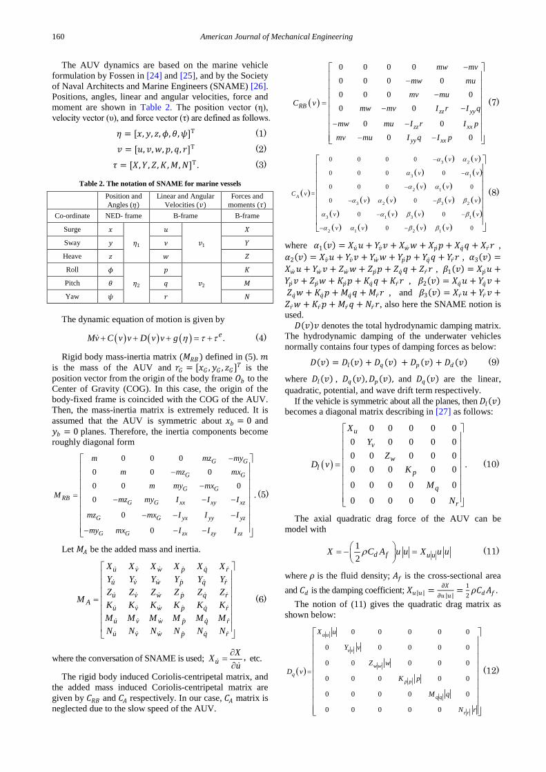
The AUV dynamics are based on the marine vehicle formulation by Fossen in [24] and [25], and by the Society of Naval Architects and Marine Engineers (SNAME) [26]. Positions, angles, linear and angular velocities, force and moment are shown in Table 2. The position vector (η), velocity vector (υ), and force vector (τ) are defined as follows.

𝜂𝜂 = [𝑥𝑥,𝑦𝑦, 𝑧𝑧,𝜙𝜙,𝜃𝜃,𝜓𝜓]T (1) 𝑣𝑣 = [𝑢𝑢, 𝑣𝑣,𝑤𝑤, 𝑝𝑝, 𝑞𝑞, 𝑟𝑟]T (2) 𝜏𝜏 = [𝑋𝑋,𝑌𝑌,𝑍𝑍,𝐾𝐾,𝑀𝑀,𝑁𝑁]T. (3)

Table 2. The notation of SNAME for marine vessels

Position and Angles (𝜂𝜂)

Linear and Angular Velocities (𝑣𝑣)

Forces and moments (𝜏𝜏)

Co-ordinate NED- frame B-frame B-frame

Surge 𝑥𝑥

𝜂𝜂1

𝑢𝑢

𝑣𝑣1

𝑋𝑋

Sway 𝑦𝑦 𝜈𝜈 𝑌𝑌

Heave 𝑧𝑧 𝑤𝑤 𝑍𝑍

Roll 𝜙𝜙

𝜂𝜂2

𝑝𝑝

𝑣𝑣2

𝐾𝐾

Pitch 𝜃𝜃 𝑞𝑞 𝑀𝑀

Yaw 𝜓𝜓 𝑟𝑟 𝑁𝑁

The dynamic equation of motion is given by

( ) ( ) ( ) .eMv C v v D v v g η τ τ+ + + = + (4)

Rigid body mass-inertia matrix (𝑀𝑀𝑅𝑅𝑅𝑅) defined in (5). 𝑚𝑚 is the mass of the AUV and 𝑟𝑟𝐺𝐺 = [𝑥𝑥𝐺𝐺 ,𝑦𝑦𝐺𝐺 , 𝑧𝑧𝐺𝐺]𝑇𝑇 is the position vector from the origin of the body frame 𝑂𝑂𝑏𝑏 to the Center of Gravity (COG). In this case, the origin of the body-fixed frame is coincided with the COG of the AUV. Then, the mass-inertia matrix is extremely reduced. It is assumed that the AUV is symmetric about 𝑥𝑥𝑏𝑏 = 0 and 𝑦𝑦𝑏𝑏 = 0 planes. Therefore, the inertia components become roughly diagonal form

0 0 0

0 0 0

0 0 0

0

0

0

.

G G

G G

G GRB

G G xx xy xz

G G yx yy yz

G G zx zy zz

m mz my

m mz mx

m my mxM mz my I I I

mz mx I I I

my mx I I I

−

−

−

− − −

− − −

− − −

=

(5)

Let 𝑀𝑀𝐴𝐴 be the added mass and inertia.

u v w p q r

u v w p q r

u v w p q rA

u v w p q r

u v w p q r

u v w p q r

X X X X X XY Y Y Y Y YZ Z Z Z Z Z

M K K K K K KM M M M M MN N N N N N

=

(6)

where the conversation of SNAME is used; uXXu

∂=∂

， etc.

The rigid body induced Coriolis-centripetal matrix, and the added mass induced Coriolis-centripetal matrix are given by 𝐶𝐶𝑅𝑅𝑅𝑅 and 𝐶𝐶𝐴𝐴 respectively. In our case, 𝐶𝐶𝐴𝐴 matrix is neglected due to the slow speed of the AUV.

( )

0 0 0 0

0 0 0 0

0 0 0 0

0 0

0 0

0 0

RBzz yy

zz xx

yy xx

mw mv

mw mu

mv muC v mw mv I r I q

mw mu I r I p

mv mu I q I p

−

−

−=

− −

− −

− −

(7)

( )

( ) ( )

( ) ( )

( ) ( )

( ) ( ) ( ) ( )

( ) ( ) ( ) ( )

( ) ( ) ( ) ( )

2

1

2 1

2 3 2

3

3

3

1 1

2 1 2

3

1

3

0 0 0 0

0 0 0 0

0 0 0 0=

0 0

0 0

0 0

A

v v

v v

v vC v

v v v v

v v v v

v v v v

α α

α α

α α

α α β β

α α β β

α α β β

−

−

−

− −

− −

− −

(8)

where 𝛼𝛼1(𝑣𝑣) = 𝑋𝑋�̇�𝑢𝑢𝑢 + 𝑌𝑌�̇�𝑣𝑣𝑣 + 𝑋𝑋�̇�𝑤𝑤𝑤 + 𝑋𝑋𝑝𝑝̇𝑝𝑝 + 𝑋𝑋�̇�𝑞𝑞𝑞 + 𝑋𝑋𝑟𝑟̇𝑟𝑟 , 𝛼𝛼2(𝑣𝑣) = 𝑋𝑋�̇�𝑣𝑢𝑢 + 𝑌𝑌�̇�𝑣𝑣𝑣 + 𝑌𝑌�̇�𝑤𝑤𝑤 + 𝑌𝑌𝑝𝑝̇𝑝𝑝 + 𝑌𝑌�̇�𝑞𝑞𝑞 + 𝑌𝑌𝑟𝑟̇𝑟𝑟 , 𝛼𝛼3(𝑣𝑣) =𝑋𝑋�̇�𝑤𝑢𝑢 + 𝑌𝑌�̇�𝑤𝑣𝑣 + 𝑍𝑍�̇�𝑤𝑤𝑤 + 𝑍𝑍𝑝𝑝̇𝑝𝑝 + 𝑍𝑍�̇�𝑞𝑞𝑞 + 𝑍𝑍𝑟𝑟̇ 𝑟𝑟 , 𝛽𝛽1(𝑣𝑣) = 𝑋𝑋𝑝𝑝̇𝑢𝑢 +𝑌𝑌𝑝𝑝̇𝑣𝑣 + 𝑍𝑍𝑝𝑝̇𝑤𝑤 + 𝐾𝐾𝑝𝑝̇𝑝𝑝 + 𝐾𝐾�̇�𝑞𝑞𝑞 + 𝐾𝐾𝑟𝑟̇𝑟𝑟 , 𝛽𝛽2(𝑣𝑣) = 𝑋𝑋�̇�𝑞𝑢𝑢 + 𝑌𝑌�̇�𝑞𝑣𝑣 + 𝑍𝑍�̇�𝑞𝑤𝑤 + 𝐾𝐾�̇�𝑞𝑝𝑝 + 𝑀𝑀�̇�𝑞𝑞𝑞 + 𝑀𝑀𝑟𝑟̇𝑟𝑟 , and 𝛽𝛽3(𝑣𝑣) = 𝑋𝑋𝑟𝑟̇𝑢𝑢 + 𝑌𝑌𝑟𝑟̇𝑣𝑣 +𝑍𝑍𝑟𝑟̇𝑤𝑤 + 𝐾𝐾𝑟𝑟̇𝑝𝑝 + 𝑀𝑀𝑟𝑟̇𝑞𝑞 + 𝑁𝑁𝑟𝑟̇𝑟𝑟, also here the SNAME notion is used. 𝐷𝐷(𝑣𝑣)𝑣𝑣 denotes the total hydrodynamic damping matrix.

The hydrodynamic damping of the underwater vehicles normally contains four types of damping forces as below:

𝐷𝐷(𝑣𝑣) = 𝐷𝐷𝑙𝑙(𝑣𝑣) + 𝐷𝐷𝑞𝑞(𝑣𝑣) + 𝐷𝐷𝑝𝑝(𝑣𝑣) + 𝐷𝐷𝑑𝑑 (𝑣𝑣) (9)

where 𝐷𝐷𝑙𝑙(𝑣𝑣) , 𝐷𝐷𝑞𝑞(𝑣𝑣),𝐷𝐷𝑝𝑝(𝑣𝑣), and 𝐷𝐷𝑞𝑞(𝑣𝑣) are the linear, quadratic, potential, and wave drift term respectively.

If the vehicle is symmetric about all the planes, then 𝐷𝐷𝑙𝑙(𝑣𝑣) becomes a diagonal matrix describing in [27] as follows:

( )

0 0 0 0 00 0 0 0 00 0 0 0 0

.0 0 0 0 0

0 0 0 0 0

0 0 0 0 0

u

v

wl

p

q

r

XY

ZD v K

M

N

=

(10)

The axial quadratic drag force of the AUV can be model with

12 d f u uX C A u u X u uρ = − =

(11)

where 𝜌𝜌 is the fluid density; 𝐴𝐴𝑓𝑓 is the cross-sectional area and 𝐶𝐶𝑑𝑑 is the damping coefficient; 𝑋𝑋𝑢𝑢 |𝑢𝑢 | = 𝜕𝜕𝑋𝑋

𝜕𝜕𝑢𝑢 |𝑢𝑢 |= 1

2𝜌𝜌𝐶𝐶𝑑𝑑𝐴𝐴𝑓𝑓 .

The notion of (11) gives the quadratic drag matrix as shown below:

( )

0 0 0 0 0

0 0 0 0 0

0 0 0 0 0

0 0 0 0 0

0 0 0 0 0

0 0 0 0 0

u u

v v

w wq

p p

q q

r r

X u

Y v

Z wD v

K p

M q

N r

=

(12)


It is considered that the weight (𝑊𝑊) of the AUV is approximately equal to the buoyance force (𝑅𝑅). 𝑘𝑘(𝜂𝜂) is the gravitational and buoyance matrix. It can be simplified as in (13) as pointed out by [24]. 𝑟𝑟𝑅𝑅 = [𝑥𝑥𝑅𝑅 , 𝑦𝑦𝑅𝑅 , 𝑧𝑧𝑅𝑅]𝑇𝑇 is the position vector for the COG to the Center of Buoyancy (COB).

( )

( ) ( )( ) ( ) ( )( ) ( ) ( )

( ) ( ) ( )( ) ( ) ( )

( ) ( ) ( ) ( ) ( )( ) ( ) ( )( ) ( )

sin

cos sin

cos

.

sin cos cos

cos

cos cos

cos sin

cos sin

sin

G B G B

G Bg v

G B

G B

G B

W B

W B

W B

z W z B x W x B

y W y B

z W z B

x W x B

y W y B

θ

θ φ

θ φ

θ θ φ

θ φ

θ φ

θ φ

θ

=

−

− −

− −

− + −

− −

+ −

− −

− −

(13)

𝜏𝜏 is the forces and moments vector of the propulsion input, and the environmental forces and moments are defined as 𝜏𝜏𝑒𝑒

The kinematic equation of the AUV can be expressed as

( )Ie Bv J R η= (14)

where 𝐽𝐽𝑒𝑒(𝑅𝑅𝑅𝑅𝐼𝐼 ) is the velocity transformation matrix between the body-fixed frame of the AUV and the earth-fixed frame and 𝑅𝑅𝑅𝑅𝐼𝐼 is the rotation matrix expressing the transformation from the earth-fixed frame to the body-fixed frame. This velocity transformation matrix is further represented as below.

( ) 3 3

3 3 ,

0

0

BI I

e Bk o

RJ R

J×

×

=

(15)

where

( )2 ,BI

c c s c s

R s c c s s c c s s s s c

s s c s c c s s s c c c

ψ θ ψ θ θ

η ψ φ ψ θ φ ψ φ ψ θ φ φ θ

ψ φ ψ θ φ ψ φ ψ θ φ φ θ

−

= − + +

+ − +

( ), 2

1 0

0

0k o

s

J c s c

s c c

θ

η φ φ θ

φ φ θ

−

=

−

and 𝑐𝑐𝛼𝛼 and 𝑠𝑠𝛼𝛼 are the short notations for cos(𝛼𝛼) and sin(𝛼𝛼), respectively.

To overcome the possible occurrence of representation singularities, it might be convenient to resort to the quaternion representation (𝑄𝑄 = {𝜀𝜀, 𝜇𝜇}) . The relationship between 𝑣𝑣, 𝜂𝜂1 and the time derivative of the quaternion �̇�𝑄 is given by the quaternion propagation equations. (See Appendix A)

3. Computational Solutions for Dynamic and Hydrodynamic Parameters

This section represents how the numerical methods are used to find the rigid body mass-inertia matrix, added mass matrix, and damping matrix. First, the SOLIDWORKS software is used to compute the mass-inertia matrix (𝑀𝑀𝑅𝑅𝑅𝑅). Next, ANSYS FLUENTTM is used to find both added mass (𝑀𝑀𝐴𝐴) and damping matrix �𝐷𝐷(𝑉𝑉)�.

3.1. Rigid Body Mass Inertia Matrix The COG and the inertia parameters of the AUV are very

difficult to calculate analytically as shown in (16) in [24] because they have many different density components. The mass and inertia of a small particle can be defined as follow.

0

2

0,

V

m

V

mm dV I r dVρ ρ= =∫ ∫ (16)

where 𝜌𝜌𝑚𝑚 is the density of an element of volume 𝑑𝑑𝑣𝑣. 𝑉𝑉 is the total volume of the AUV, 𝑟𝑟 is the distance between the element of volume 𝑑𝑑𝑣𝑣 and the COG.

The best way to calculate the mass-inertia matrix (𝑀𝑀𝑅𝑅𝑅𝑅) of the AUV is to use the CAD software, SOLIDWORKS. The SOLIDWORKS’ model of the AUV is shown in Figure 1 and 𝑀𝑀𝑅𝑅𝑅𝑅 is listed in (17). Floating and payloads are not examined here. It is acceptable to neglect the off-diagonal inertia elements compared with the diagonal terms, expressed as follows. The units are measured in 𝑘𝑘𝑘𝑘 and 𝑘𝑘𝑘𝑘𝑚𝑚2.

16.247 0 0 0 0 0

0 16.247 0 0 0 0

0 0 16.247 0 0 0

0 0 0 0.2568 0 0

0 0 0 0 0.3841 0

0 0 0 0 0 0.3716

.RBM =

(17)

3.2. Added Mass Matrix The added mass of the AUV really depends on the

geometry of the underwater vehicle as mentioned in [28]. Hence, the use of empirical formulas predicting 𝑀𝑀𝐴𝐴 and a hull approximation by elementary shapes are inaccurate for the complex-shaped AUV. For the case of a complex-shaped AUV, 𝑀𝑀𝐴𝐴 matrix cannot pursue the empirical formulas noted in [5] and [6]. ANSYS FLUENTTM is advanced to compute the hydrodynamic characteristics of marine objects, offering the function to figure out the added mass matrix, and it requires a closed geometry of the AUV for the calculation. In this case, the speed of the AUV is low enough to neglect the off-diagonal elements. Thus, the diagonalized matrix is considered for the MATLAB simulations done in Section 4 and Section 5. The units are measured in 𝑘𝑘𝑘𝑘 and 𝑘𝑘𝑘𝑘𝑚𝑚2.

12.713 0.103 0.115 0.042 0.318 0.017

0.158 21.827 0.156 0.087 0.019 0.785

0.138 0.151 69.689 0.039 0.723 0.072

0.143 0.405 0.063 0.524 0.004 0.016

0.507 0.004 0.742 0.005 0.971 0.004

0.008 0.796 0.082 0.006 0.006 0.212

AM =

− −

− − −

− −

− −

− −

− − −

(18)

3.3. Damping Matrix In this case, 𝐷𝐷𝑝𝑝(𝑣𝑣) can be neglected comparing to other

terms, and 𝐷𝐷𝑑𝑑(𝑣𝑣) is also ignored since the AUV operates under certain depth, shown in [24].


These formulas are impractical to calculate the damping matrix. Hence, ANSYS FLUENTTM based on the finite element theory is used to compute the relationship between the damping forces and velocity of the AUV. The AUV is fixed in a rectangular tank in which the velocity of the fluid varies from 0 to 0.6 𝑚𝑚/𝑠𝑠 (approximation of general AUV operating speed), with the speed interval of 0.1 𝑚𝑚/𝑠𝑠.

The velocity stream-line views of ANSYS FLUENTTM results in different directions are shown in Figure 3. The configuration details used for the simulation are listed in Table 3, and the computed damping forces and moments are listed in Table 4 and Table 5. A second order polynomial relationship is noticed between damping forces/moments and velocities, see Figure 4 and Figure 5.

Figure 3. ANSYS FLUENTTM velocity streamline views of the AUV at 0.5 m/s: (a) in surge direction; (b) in sway direction; (c) in heave direction

Table 3. Configuration details of ANSYS FLUENTTM

Parameter Description

Tank 12𝑚𝑚 (L) 5𝑚𝑚 (W) 5𝑚𝑚 (H)

Fluid Sea water. Viscosity= 1.60 × 10−6 𝑘𝑘𝑘𝑘/(𝑠𝑠𝑚𝑚) at 5℃ and salinity 4%, density = 1023 𝑘𝑘𝑘𝑘/𝑚𝑚3

Turbulence Sheer stress transport 1% at inlet boundary

Mesh size 596455 elements

Convergence 6 × 10−5

Roughness 0.0015− 0.009 𝑚𝑚𝑚𝑚

Table 4. Damping forces at different linear velocities

Linear velocity/(𝑚𝑚/𝑠𝑠) 0.1 0.2 0.3 0.4 0.5 0.6

Surge/(𝑁𝑁) 0.322 1.287 2.893 5.141 8.032 11.564

Sway/(𝑁𝑁) 0.563 2.253 5.069 9.013 14.080 20.275

Heave/(𝑁𝑁) 0.736 2.943 6.622 11.773 18.395 26.488

Table 5. Damping torques at different angular velocities

Angular velocity/(𝑟𝑟𝑟𝑟𝑑𝑑/𝑠𝑠) 0.5 1 1.5 2 2.5 3

Roll/(𝑁𝑁𝑚𝑚) 0.120 0.387 0.800 1.360 2.066 2.919

Pitch/(𝑁𝑁𝑚𝑚) 0.319 0.904 1.754 2.870 4.251 5.898

Yaw/(𝑁𝑁𝑚𝑚) 0.149 0.470 0.964 1.630 2.469 3.480

Figure 4. Estimated damping force with linear velocity

Figure 5. Estimated damping torque with angular velocity

0.5 1 1.5 2 2.5 30

1

2

3

4

5

6


4. Trajectory Tracking Control Law

The dynamics of the AUV denoted in (4) include the uncertainty of the parameters in the damping matrix. It is designed to recompense the uncertainties; therefore, the vehicle-fixed-frame adaptive controller is proposed to achieve a consistent AUV performance by estimating uncertain parameters. The parameters in the control law are adjusted by an adaption mechanism. The proposed adaptive controller is designed to force the AUV to follow the desired trajectory with the existence of a parameter uncertainty. For this, a regression matrix should be defined.

Let us consider the vehicle-fixed variables

1BIy R ηε

=

(19)

dv v v= − (20)

where 𝜂𝜂�1 = 𝜂𝜂1 − 𝜂𝜂1,𝑑𝑑 being 𝜂𝜂1,𝑑𝑑 the desired position, and the quaternion-based attitude error is given by 𝜀𝜀̃. 𝑣𝑣𝑑𝑑 is the desired velocity of the AUV in the body-fixed frame.

The error vector is given by:

𝑆𝑆=𝑣𝑣+Λ𝑦𝑦 (21) with Λ = positive definite matrix.

The vehicle regressor matrix

( )Φ Φ , , ,d dv v v v= (22)

The adaptive control law can be defined in the following form.

( ) ˆτ Φ , , , Θ .d d Dv v v v K S= + (23)

Such that,

( ) ( ) ( )

( ) ˆΦ , , , Θd d d

d d D

Mv C v v D v v g

v v v v K S

η+ + +

= +

(24)

where 𝐾𝐾𝐷𝐷 is a (6 × 6) positive definite matrix. The parameter estimate Θ� is updated by

TΘ̂ ΓΦ S= (25) where Γ is a suitable positive definite matrix of an appropriate dimension, and is selected in such a way that the tuning law provides convergent characteristics.

The adaptive law proposed in the equation can drive the AUV in a desired manner, and guarantee the AUV’s stability. The structure of the proposed control is given in the block diagram below.

Figure 6. MATLAB SIMULINK layout of the proposed adaptive control law

4.1. Stability of the Proposed Control Law The following Lyapunov candidate function is used to

examine the stability of the system.

( ) ( ) ( )T 1

1 21 Θ Γ Θ ,2

ˆΘ Θ Θ, 0, Θ 0

TV t S MS V t V t

S

− = + = +

= − ∀ ≠ ≠

(26)

where 𝑉𝑉1(𝑡𝑡) = 12𝑆𝑆T𝑀𝑀𝑆𝑆 and 𝑉𝑉2(𝑡𝑡) = 1

2Θ�TΓ−1Θ�.

The selected Lyapunov candidate function satisfies the conditions given in (27).

( )( ) ( )

( ) ( )0, 0 ( )

:

0, 0

n

dV tV t if and only if t negative definite

dt

V t R R such that

V t if and only if t positive definite

= ≤ =

→

≥ =

(27)

Indeed, the system is asymptotically stable in the sense of Lyapunov because 𝑉𝑉(𝑡𝑡) satisfies the above conditions.

The time derivative of (26) is given by

( ) ( ) ( )1 1V t V t V t= + (28)

Being 𝑉𝑉1̇(𝑡𝑡) and 𝑉𝑉2̇(𝑡𝑡) as follows,

( ) T T1

12

V t S MS S M= + (29)

( ) T 12 Θ̂ Γ ΘV t −= (30)

where Θ�̇ = Θ̇� + 0, as Θ is a constant definite vector Substituting (21) into (29), as shown in [29].

( ) ( )T T1

12dV t S M v v S MS= − +

(31)

where 𝑆𝑆 = 𝑣𝑣𝑑𝑑 − 𝑣𝑣 Substituting the value of 𝑀𝑀�̇�𝑣 from (4) into (31) and

simplifying for 𝑉𝑉1̇(𝑡𝑡)

( ) ( )T T1

12dV t S Mv Cv Dv g S MSτ= + + + − +

(32)

( )( )

( )T T

112

d d

d

Mv C s vV t S S MS

D s v g τ

+ − += + + − + + −

(33)

( ) ( )

( )( )( )

T1

T1 22

d d dV t S Mv Cv Dv g

S M C D S

τ= + + + −

+ − +

(34)

�̇�𝑀 − 2(𝐶𝐶 + 𝐷𝐷) is a skew-symmetric matrix for the AUVs. Substituting the system dynamics given in (4) into above equation.

( ) ( )T1 ΘV t S Y τ= − (35)

Therefore, equation (28) becomes,

( ) ( )T T 1ˆΘ̂ Θ Γ ΘV t S Y τ −= − + (36)

Substituting the control input (𝜏𝜏) into (36)

( ) ( )T T 1ˆΦΘ ΦΘ Θ̂ Γ ΘDV t S K S −= − − + (37)


�̇�𝑉(𝑡𝑡) = 𝑆𝑆T�−ΦΘ� − 𝐾𝐾𝐷𝐷𝑆𝑆� + Θ̇�TΓ−1Θ� (38)

�̇�𝑉(𝑡𝑡) = −𝑆𝑆TΦΘ� − 𝑆𝑆T𝐾𝐾𝐷𝐷𝑆𝑆 + Θ̇�TΓ−1Θ�. (39)

Substituting Θ̇� from (25) into (39)

�̇�𝑉(𝑡𝑡) = −𝑆𝑆TΦΘ� − 𝑆𝑆T𝐾𝐾𝐷𝐷𝑆𝑆 + (ΓΦT𝑆𝑆)TΓ−1Θ� (40) �̇�𝑉(𝑡𝑡) = −𝑆𝑆T𝐾𝐾𝐷𝐷𝑆𝑆 ≤ 0 (41)

Equation (41) satisfies the Lyapunov stability criterion of the AUV dynamics with a stable controller. Therefore, the adaptive control law proposed in (23) gives a stable closed system.

4.2. Validation of the Adaptive Controller The derivation of the regressor matrix of a high-DOF is

very cumbersome. Therefore, for the sake of simplicity, only five DOFs are considered.

𝑀𝑀�̇�𝑣𝑑𝑑 + 𝐷𝐷𝑣𝑣𝑑𝑑 = 𝜏𝜏 (42) where

( )11 22 33 44 55 ,M diag m m m m m= + + + +

( )11 22 33 44 55 ,D diag d d d d d= + + + +

𝑣𝑣𝑑𝑑 = [𝑢𝑢𝑑𝑑 ,𝑢𝑢𝑑𝑑 ,𝑤𝑤𝑑𝑑 , 𝑞𝑞𝑑𝑑 , 𝑟𝑟𝑑𝑑 ]T , and 𝜏𝜏 = ΦΘ� + 𝐾𝐾𝐷𝐷𝑆𝑆. When the regression matrix Φ is used, the AUV model

given in (42) can be written down in the form of linear

parameters. For a real-time implementation, it is clear that the regression matrix, a state dependent matrix, is needed to calculate in each control cycle, seen in [30].

The regression matrix defined in (22) can be written as follows:

( )0 0 0 0 0 0 0 0

0 0 0 0 0 0 0 0

0 0 0 0 0 0 0 0

0 0 0 0 0 0 0 0

0 0 0 0 0 0 0 0

,

d d d

d d d

d d d

d d d

d d d

d d

u u u

v v v

w w w

q q q

r r r

vν

=

Φ

(43)

The number of simulations is performed with the desired trajectories to check the validity of the proposed control. The parameters of the AUV used for simulations are listed in Table 6.

The desired trajectory in the form of a circular path.

( )( ) ( )

5sin 0.02 ,

5cos 0.02 , 0.5sin 0.02 ,

, ,4 6

d

d d

d d

x t

y t z tπ πθ ψ

=

= =

= =

(44)

Note: The selected trajectory functions should be continuous to compute the second derivative with respect to time.

Figure 7. Circular trajectory comparison between the desired path and actual path projected onto: (a) 𝑥𝑥𝑦𝑦 plane; (b) 𝑥𝑥𝑧𝑧 plane and plotted; (c) in ℝ3 space


Table 6. Parameters of the AUV used for the simulation

Mass/(𝑘𝑘𝑘𝑘,𝑘𝑘𝑘𝑘𝑚𝑚2) Damping coefficient/(𝑘𝑘𝑘𝑘/𝑠𝑠 ,𝑘𝑘𝑘𝑘𝑚𝑚2/𝑠𝑠) Gain matrix 𝑚𝑚11=28.960 𝐷𝐷11 = 32.1𝑢𝑢2 + 0.013|𝑢𝑢| 𝐾𝐾𝐷𝐷 = 𝑑𝑑𝑑𝑑𝑟𝑟𝑘𝑘([10, 15, 40, 10,10]) 𝑚𝑚22=38.074 𝐷𝐷22 = 56.32𝑣𝑣2 Λ = 𝑑𝑑𝑑𝑑𝑟𝑟𝑘𝑘([45, 15, 20, 20,20]) 𝑚𝑚33=85.936 𝐷𝐷33 = 73.58𝑤𝑤2

Γ = 𝑑𝑑𝑑𝑑𝑟𝑟𝑘𝑘([170, 15, 30,20,30,20,10,10,10,10]) 𝑚𝑚44=1.355 𝐷𝐷44 = 0.531𝑞𝑞2 + 0.373|𝑞𝑞| 𝑚𝑚55=0.584 𝐷𝐷55 = 0.345𝑟𝑟2 + 0.125|𝑟𝑟|

Figure 8. Actual position and attitude of the AUV compared with the desired position and attitude: (a) after 120 𝑠𝑠; (b) after 630 𝑠𝑠

Figure 9. Earth-fixed linear and angular velocities: (a) after 120 𝑠𝑠; (b) after 630 𝑠𝑠

Figure 8 elaborates that the actual position and orientation of the AUV accurately track the desired position and orientation after 95 𝑠𝑠.

Figure 10. Position and attitude errors of the AUV after 200 𝑠𝑠

Figure 9 illustrates that the velocity errors tended to

zero within 85 𝑠𝑠 from the beginning. And also, Figure 10 and Figure 11 asymptotically converge to zero. Thus, the proposed controller accurately commands the AUV to follow the desired path.

Figure 11. Earth-fixed frame velocity errors of the AUV after 200 𝑠𝑠

0 20 40 60 80 100 120 140 160 180 200-1

0

1

2

3

4

5

0 20 40 60 80 100 120 140 160 180 200-0.5

-0.4

-0.3

-0.2

-0.1

0

0.1


Figure 12. Forces and torques applied to the AUV: (a) after 50 𝑠𝑠; (b) after 630 𝑠𝑠

In Figure 12, it is true that initially, both forces and torques have some definite values showing that the AUV accomplished the required acceleration, but after 30 𝑠𝑠, the torques in case of pitch and yaw converged to zero, which means the angular accelerations became to zero. The forces in case of surge, sway and heave indicate the simple harmonic variation around zero to catch the sinusoidal position inputs, which include the high amplitude in these directions.

5. AUV Path Planning with Optimum Thrust Allocation

5.1. Path Planning Algorithm Using the Adaptive Control Law

In this case, according to the thrust placement given in Figure 1, there are 4 DOFs: surge, roll, pitch, and yaw, in which the AUV is able to maneuver with the controller inputs for the surge 𝑢𝑢𝑑𝑑 , roll ∅𝑑𝑑 , pitch 𝜃𝜃𝑑𝑑 , and yaw 𝜓𝜓𝑑𝑑 DOFs, but the roll DOF behaves like a self-stabilizer. This AUV can move from its current position, called set-point A, to desired potion, called set-point B as shown in Figure 13.

Figure 13. Visualization of the coordinate parameters

The desired point 𝑩𝑩 is always considered as the origin of the frame that is parallel to the earth fixed frame, while the origin of the body-fixed frame which coincides with the COG is the current position 𝑨𝑨 . The error vector

𝑒𝑒(𝑡𝑡) = [𝑒𝑒1, 𝑒𝑒2, 𝑒𝑒3]T describes the position error between the desired point and the current location of the AUV, as shown in Figure 13. The control inputs are provided to steer the AUV along the instantaneously desired path 𝑒𝑒(𝑡𝑡) as the optimum path between 𝑨𝑨 and 𝑩𝑩 to minimize the 𝑒𝑒(𝑡𝑡). The AUV is also guided asymptotically towards the desired point 𝑩𝑩 . Note that this control inputs are only

valid for ,2eπθ ≠ and .

2eπψ ≠

( ) 1 1B Ae t η η= − (45)

( )( ) ( )

; ,cos cosd e d e d

e e

ke tu θ θ θ ψ ψ ψ

θ ψ= = − = − (46)

0d∅ = (47)

1 3

1tand

ee

θ − =

(48)

( )( )( )2 1mod 2 , 2 ,2 ; 0 2d datan e eψ π π ψ π= + ≤ ≤ (49)

[ ]2, , , .Td d d dη θ ψ= ∅ (50)

where 𝑘𝑘 is a positive constant. This control model has the position controller, attitude

controller, speed controller and plant (AUV). The desired and current position given in the earth fixed frame are the inputs for the position controller which gives the desired attitude 𝜂𝜂2,𝑑𝑑 , and 𝑒𝑒 as the outputs. The controller discussed in Section 4 is based on the body-fixed frame. Thus, all the inputs for the adaptive controller should be converted to the body-fixed frame. The outputs of the attitude controller are the desired propulsion torques in the roll, pitch, and yaw directions 𝜏𝜏𝑑𝑑 ,4−6 . Furthermore, 𝑒𝑒, 𝑣𝑣, and 𝜂𝜂�2 are the inputs for the speed controller giving the propulsion force in the surge direction 𝜏𝜏𝑑𝑑 ,1 as the output. The inputs of the plant are 𝜏𝜏𝑑𝑑 ,1 , 𝜏𝜏𝑑𝑑 ,4−6 , 𝑣𝑣, and �̇�𝑣 , see Figure 14.

The MATLAB SIMULINK block diagram of this controller is shown in below.


Figure 14. MATLAB SIMULINK layout of the controller

5.2. Optimum Thrust Allocation In the thrust allocation, optimizing methods are

used to minimize the thrust forces to save the power consumption and increase the efficiency of the AUVs. This complex-shaped underwater vehicle contains 6 thrusters and they allow to control the four DOFs: surge, roll, pitch, and yaw. The thruster configuration, thruster forces, thruster numbering and distances are shown with respect to the body-fixed frame in Figure 15.

Figure 15. Location of the thrusters on the AUV, definition of the distances, and direction of the positive thrust

The force and torque vector can be defined as follows, seen in [25,31]:

𝜏𝜏 = 𝑇𝑇𝑓𝑓 (51) where 𝑇𝑇 is the thruster configuration matrix, indicating the direction of the force in the surge DOF, and the direction of the toques in the roll, pitch, and heave DOFs,

1 1 1 1

5 5 2 2 3 3

4 4

1 1 0 0 0 00 0

0 0 0 0

L L L LT

L L L L L LL L

− − = − −

−

(52)

here, the distances 𝐿𝐿𝑑𝑑 are 𝐿𝐿1 = 𝐿𝐿4 = 154 𝑚𝑚𝑚𝑚, 𝐿𝐿2 = 𝐿𝐿3 =210 𝑚𝑚𝑚𝑚 , and 𝐿𝐿5 = 90 𝑚𝑚𝑚𝑚 , and also 𝑓𝑓 is the thrust vector.

𝑓𝑓 = [𝑓𝑓1 𝑓𝑓2 𝑓𝑓3 𝑓𝑓4 𝑓𝑓5 𝑓𝑓6]𝑇𝑇 (53) The optimum thrust allocation from the required 𝜏𝜏 can

be considered as a model-based optimization problem and it can be categorized under two major categories: constrained thrust allocation and unconstrained thrust allocation. For this AUV, the unconstrained thrust

allocation is used because it does not pay an attention about the bounded limitations (minimum and maximum) for the thrust vector. This approach has several advantages than the constrained thrust allocation; it consumes minimum computational time, and requires an on-board computer with low computational power. Assumption:

The vector of propulsion forces and torques 𝜏𝜏 is bounded in such a way that the computed elements of the thrust vector 𝑓𝑓 never exceed the boundary values of 𝑓𝑓𝑚𝑚𝑑𝑑𝑚𝑚 and 𝑓𝑓𝑚𝑚𝑟𝑟𝑥𝑥 .

Under above assumption, this thrust allocation can be expressed as a problem of the least-squares optimization as follows:

1min2

Tf Hf (54)

where 𝐻𝐻 is a positive definite matrix. The solution of (54) using Lagrange multipliers shown

in [25] is given by

𝑓𝑓𝑜𝑜𝑝𝑝𝑡𝑡 = 𝑇𝑇∗ 𝜏𝜏 (55)

𝑇𝑇∗ = 𝐻𝐻−1𝑇𝑇𝑇𝑇(𝑇𝑇𝐻𝐻−1𝑇𝑇𝑇𝑇)−1 (56) This approach provides a suitable solution for the

faultless work of the propulsion system, and cannot be used directly in case of damaged thrusters.

5.2.1. Singular Value Decomposition (SVD) for the Solution

SVD is an eigenvalue-like decomposition for rectangular matrices [32]. After applying the SVD for the thrust configuration matrix, it becomes as follows:

𝑇𝑇 = 𝑈𝑈𝑆𝑆𝑉𝑉𝑇𝑇 (57) where 𝑈𝑈 and 𝑉𝑉 are orthogonal matrices of dimensions 4 × 4 and 𝑚𝑚 × 𝑚𝑚, respectively. 𝑚𝑚 is the number of thrusters in the AUV.

[ ]1

2

3

4

0 0 00 0 0

|O , .0 0 00 0 0

T TS S S

γγ

γγ

= =

(58)

𝑆𝑆T- diagonal matrix of dimensions 4 × 4 O- null matrix of dimensions 4 × (𝑚𝑚 − 4).


The singular values of 𝑇𝑇, called 𝛾𝛾1, 𝛾𝛾2, 𝛾𝛾3 and 𝛾𝛾4 , are positive and the order of them should be like 𝛾𝛾1 ≥ 𝛾𝛾2 ≥𝛾𝛾3 ≥ 𝛾𝛾4. To calculate the optimum thrust vector 𝑓𝑓𝑜𝑜𝑝𝑝𝑡𝑡 being a minimum-norm solution to (54), the decomposition form of 𝑇𝑇 is necessary to compute. Finally, 𝑓𝑓𝑜𝑜𝑝𝑝𝑡𝑡 can be written in the form of

1

.O

TTopt

Sf V U τ−

=

(59)

5.3. Simulation Results and Discussion In this section, we present the simulation results of the

path planning algorithm and the optimized thrust allocation defined in Section 5.1 and Section 5.2 respectively, including the uncertainty of the hydrodynamic parameters. To simulate the proposed path following algorithm, the

AUV requires the earth-fixed frame co-ordinates of the set-point A and B for the path planning. It starts form the set-point A (-8, -8, -2) and is driven through the co-ordinates of the set-point B, see Table 7. All of these points were randomly selected for the simulation. The AUV automatically selects the next set point B in the sequence given in Table 7. Figure 16 a) and Figure 16 b) show the projection of the path that the AUV followed onto 𝑥𝑥𝑦𝑦 and 𝑥𝑥𝑧𝑧 plane, respectively. Figure 16 c) presents the path of the AUV in ℝ3 space.

Table 7. Coordinates of set-point B denoted in the earth-fixed frame

Position of the AUV Co-ordinates of set-point B

𝑥𝑥𝑅𝑅 -3 2 5 8 5 0

𝑦𝑦𝑅𝑅 -2 -5 5 7 2 -1

𝑧𝑧𝑅𝑅 0 1 2 0 1 3

Figure 16. Path of the AUV drawn by its COG: (a) projected onto 𝒙𝒙𝒙𝒙 plane; (b) projected onto 𝒙𝒙𝒙𝒙 plane; (c) in ℝ𝟑𝟑 space

Figure 17. Desired and actual position of the path in the earth-fixed frame

Figure 18. Position error of the path in the earth-fixed frame

0 50 100 150 200 250 300 350 400 450-8

-6

-4

-2

0

2

4

6

8

10


The comparison between the desired and actual position is given in Figure 17. The Position error converges to zero at each set-point B, and just after that it increases to match with the new error, as shown in Figure 18.

Figure 19. Desired and actual attitude of the path in the earth-fixed frame

Figure 20. Desired and actual attitude error of the path in the earth-fixed frame

Figure 19 illustrates the desired and actual attitude. In the attitude error given in Figure 20, it is observed that the roll angle always tries to maintain its value around zero like a self-stabilizer. It is important to note that the pitch and yaw angles always vary to match with the optimum path between the current position A and the set-point B.

Figure 21. Force and torques applied to the AUV

The Propulsion force in the surge direction and torques in the roll, pitch and yaw directions are indicated in Figure 21. The force and the torques suddenly increase

just after reaching each set-point B since the position and attitude errors instantly grow due to the new target, but they asymptotically converge to zero within 50 𝑠𝑠 , indicating that linear and angular velocities become constant. Thus, we can assume that the AUV runs towards the next set-point B smoothly. 𝐻𝐻,𝑇𝑇,𝑈𝑈,𝑉𝑉, and 𝑆𝑆T are calculated as below using (57) to

compute the optimum thrust allocation for the above discussed AUV;

𝐻𝐻 =

⎣⎢⎢⎢⎢⎡1 0 0 0 0 00 1 0 0 0 00 0 1 0 0 00 0 0 1 0 00 0 0 0 1 00 0 0 0 0 1⎦

⎥⎥⎥⎥⎤

(60)

1 1 0 0 0 0

0 0 0.154 0.154 0.154 0.154

0.090 0.090 0.210 0.210 0.210 0.210

0.154 0.154 0 0 0 0

T− −

=− −

−

(61)

0.9952 0.0981 0 00 0 1 0

0.0981 0.9952 0 00 0 0 1

U

− = − −

−

(62)

0.7068 0.0205 0 0.7071 0 0

0.7068 0.0205 0 0.7071 0 0

0.0145 0.4998 0.5000 0 0.1000 0.7000

0.0145 0.4998 0.5000 0 0.7000 0.1000

0.0145 0.4998 0.5000 0 0.7000 0.1000

0.0145 0.4998 0.5000 0 0.1000 0.7000

V

− −

−

− −=

− − − −

−

−

(63)

1.4205 0 0 00 0.4181 0 0

.0 0 0.3080 00 0 0 0.2178

TS

=

(64)

Figure 22. Optimum thrust forces acting on 6 thrusters

The optimum thrust forces 𝑓𝑓𝑜𝑜𝑝𝑝𝑡𝑡 derived in (59) are shown in Figure 22. This figure indicates the variation of the thrust vector under the assumption of the unconstrained thrust allocation as discussed in Section 5.2. Generally, 𝑓𝑓1 and 𝑓𝑓2 are much higher than the others

0 50 100 150 200 250 300 350 400 450

-150

-100

-50

0

50

100

150


since they provide the propulsion force in the surge direction. Particularly, at the beginning of each new set-point B, all the thrusters show their peak thrust forces. And also, each pair of the thrusters acts in the opposite direction to create the moments for at least one attitude.

6. Conclusion

By avoiding the expensive devices, this paper presents the numerical solution to find the hydrodynamic parameters and it showed that the damping is varied in the quadratic form leading the non-linearity in the AUV model, which should be carefully considered when any linear based controller is designed. Furthermore, an adaptive control law is proposed to track the trajectories, including the uncertainty of the hydrodynamic parameters and using quaternion-based attitude error. Lyapunov’s direct approach is used to verify the stability of the proposed control law. It is also developed to plan the optimum path through the given co-ordinates using the concept of the convergence of geometric errors. Finally, an algorithm based on the decomposition of the thrust configuration matrix is used to optimize the unconstrained thrust allocation for the given six thrusters' configuration. The accuracy of the developed control law is verified by the results of the numerical simulation.

Appendix A

By defining the mutual orientation between two frames of common origin of the rotation matrix.

𝑅𝑅𝑚𝑚(𝛿𝛿) = 𝐼𝐼3 + 𝑠𝑠𝑑𝑑𝑚𝑚(𝛿𝛿) 𝑚𝑚� + (1 − 𝑐𝑐𝑜𝑜𝑠𝑠(𝛿𝛿))𝑚𝑚�2 (65) where 𝛿𝛿 is the angle and 𝑚𝑚 𝜖𝜖 ℝ𝟑𝟑 is the unit vector of the axis expressing the rotation needed to align the two frames. �̂�𝑝 is the matrix operator performing the cross product between two (3 × 1) vectors.

�̂�𝑝 = �0 −𝑝𝑝3 𝑝𝑝2𝑝𝑝3 0 −𝑝𝑝1−𝑝𝑝2 𝑝𝑝1 0

� (66)

The unit quaternion is

{ },Q ε µ= (67)

with

, cos2 2

nsin δ δε µ = =

(68)

where 𝜇𝜇 ≥ 0 for 𝜀𝜀 = [−𝜋𝜋,𝜋𝜋] 𝑟𝑟𝑟𝑟𝑑𝑑. The unit quaternion satisfies the condition

𝜇𝜇2 + 𝜀𝜀𝜀𝜀T = 1 (69) Let’s define the vector 𝜂𝜂𝑞𝑞𝝐𝝐ℝ𝟕𝟕 as follows:

1q Q

ηη

=

(70)

The relationship between 𝑣𝑣 and �̇�𝜂𝑞𝑞 is given as follows:

( )q qv J Q η= (71)

where

( )( )

( )3 4

3 3 ,

0

0 4

BI

q Tk oq

R QJ Q

J Q×

×

=

(72)

( )

( ) ( ) ( )

( ) ( ) ( )

( ) ( ) ( )

2 22 3 1 2 3 1 3 2

2 21 2 3 1 3 2 3 1

2 21 3 2 2 3 1 1 2

1 2 2 2

2 1 2 2

2 2 1 2

BIR Q

ε ε ε ε ε ε ε ε



µ µ

µ µ

µ µ

− + + −

= − − + +

+ − − +

(73)

and

( )

3 2

3 1, , , 3

2 1

1 2 3

1,4

Tk oq k oq k oqJ Q J J I

ε εε εε ε

µ

ε ε

µµε

− − = = − − − −

(74)

References [1] I. Yamamoto, "Robust and non-linear control of marine system,"

International Journal of Robust and Nonlinear Control, 11 (13), 1285-1341, Aug.2001.

[2] B. M. Ferreira, A. C. Matos, and N. A. Cruz, "Modeling and control of trimares auv," in 12th International Conference on Autonomous Robot Systems and Competitions, Portugal, 57-62 April 2012.

[3] Berge S. and Fossen T.I., "Robust control allocation of over actuated ships: Experiments with a model ship," in 4th IFAC Conference on Manoeuvring and Control of Marine Craft, Brijuni, Croatia, 161-171.

[4] M. Caccia, G. Indiveri, and G. Veruggio, "Modeling and identification of open-frame variable configuration unmanned underwater vehicles," IEEE Journal of Oceanic Engineering, 25 (2), 227-240, 2000.

[5] M. E. Rentschler, F. S. Hover, and C. Chryssostomidis, "Modeling and control of an odyssey iii auv through system identification tests," in Conference on Unmanned Untethered Submersible Technology, Durham, USA, Aug.2003.

[6] B. Ferreira, M. Pinto, A. Matos, and N. Cruz, "Hydrodynamic modeling and motion limits of auv mares," in 35th Annual Conference of IEEE on Industrial Electronics, Proto, 2241-2246.

[7] Y.H. Eng, M.W. Lau, and C.S. Chin, "Added mass computation for control of an open-frame remotely-operated vehicle: Application using WAMIT and MATLAB," Marine Science and Technology, 22 (2). 1-14, 2013.

[8] Y. H. Eng, W. S. Lau, E. Low, and G. G. L. Seet, " Identification of the hydrodynamics coefficients of an underwater vehicle using free decay pendulum motion," in International Multiconference of Engineers and Computer Scientists, Hong Kong, Vol.2, 423-430, March 2008.

[9] L. Wang, H. M. Jia, L. J. Zhang, H. B. Wang., "Horizontal tracking control for AUV based on nonlinear sliding mode," in IEEE International Conference on Information and Automation (ICIA), IEEE, Shenyang, China, 460-463, 2012.

[10] F. Repoulias, E. Papadopoulos, "Planar trajectory planning and tracking control design for underactuated AUVs," Ocean Engineering, 34 (11), 1650-1667, 2007.

[11] W. Caharija, K. Y. Pettersen, J. T. Gravdahl, E. Borhaug, "Path following of underactuated autonomous underwater vehicles in the presence of ocean currents," in 51st IEEE Conference on Decision and Control (CDC), IEEE, Maui, HI, USA, 528-535, 2012.

[12] F. D. Gao, C. Y. Pan, Y. Y. Han, X. Zhang, "Nonlinear trajectory tracking control of a new autonomous underwater vehicle in complex sea conditions," Journal of Central South University, 19 (7), 1859-1868, 2012.


[13] R. N. Smith, Y. Chao, P. P. Li, D. A. Caron, B. H. Jones, G. S. Sukhatme, "Planning and implementing trajectories for autonomous underwater vehicles to track evolving ocean processes based on predictions from a regional ocean model," International Journal of Robotics Research, 29 (12). 1475-1479, 2010.

[14] D. Chwa, "Fuzzy adaptive tracking control of wheeled mobile robots with state-dependent kinematic and dynamic disturbances," IEEE Transactions on Fuzzy Systems, 20 (3). 587-593, 2012.

[15] X. Q. Bian, J. J. Zhou, Z. P. Yan, H. N. Jia, "Adaptive neural network control system of path following for AUVs," in Proceedings of the Southeastcon, IEEE, Orlando, FL, USA, 1-5, 2012.

[16] B. B. Miao, T. S. Li, W. L. Luo, "A DSC and MLP based robust adaptive NN tracking control for underwater vehicle," Neurocomputing, 111, 184-189, 2013.

[17] O. Mohareri, R. Dhaouadi, A. B. Rad, "Indirect adaptive tracking control of a nonholonomic mobile robot via neural networks," Neurocomputing, 88, 54-66, 2012.

[18] B. Garau, M. Bonet, A. ´Alvarez, S. Ruiz, A. Pascual, "Path planning for autonomous underwater vehicles in realistic oceanic current fields: Application to gliders in the western Mediterranean Sea," Journal of Maritime Research, 6 (2), 5-21, 2009.

[19] D. Kruger, R. Stolkin, A. Blum, J. Briganti, "Optimal AUV path planning for extended missions in complex, fast-flowing estuarine environments," in IEEE International Conference on Robotics and Automation, IEEE, Roma, Italy, 4265-4270, 2007.

[20] J. Ghommam, O. Calvo, A. Rozenfeld, "Coordinated path following for multiple underactuated AUVs," in International Conference of OCEANS MTS/IEEE Kobe Techno-Ocean, IEEE, Kobe, Japan, 1-7, 2008.

[21] H. Bo, R. Hongge, Y. Ke, H. Luyue, R. Chunyun, "Path planning and tracking for autonomous underwater vehicles," in IEEE

International Conference on Information and Automation, IEEE, Zhuhai/Macau, China, 728-733, 2009.

[22] X. B. Xiang, L. Lapierre, C. Liu, B. Jouvencel. "Path tracking: Combined path following and trajectory tracking for autonomous underwater vehicles," in IEEE/RSJ International Conference on Intelligent Robots and Systems, IEEE, San Francisco, USA, 3558-3563, 2011.

[23] GrabCAD community. Available: https://grabcad.com/library/rov-54 (accessed on 20 April 2019).

[24] Thor I. Fossen, Marine control systems: guidance, navigation and control of ships, rigs and underwater vehicles, Marine Cybernetics Trondheim, Norwasy, 2002.

[25] Thor I. Fossen, Guidance and Control of Ocean Vehicles, Wiley, New York, 1994.

[26] SNAME, Nomenclature for treating the motion of a submerged body through a fluid, The Society of Naval Architects and Marine Engineers, New York, 1950.

[27] W. Wang and C. M. Clark, Modeling and Simulation of the Video Ray Pro III Underwater Vehicle, University of Waterloo, Canada, 2001.

[28] D. Perrault, N. Bose, S. O’Young, and C. D. Williams, "Sensitivity of auv added mass coefficients to variations in hull and control plane geometry," Ocean engineering, 30 (5), 645-671, 2003.

[29] J. J. E. Slotine, W. Li, Applied Nonlinear Control, Englewood Cliffs, NJ: Prentice-Hall, 1991.

[30] A. C. Huang, M. C. Chien, Adaptive Control of Robot Manipulators: A Unified Regressor-free Approach, Singapore: World Scientific Publishing Company, 2010.

[31] J.Garus, " Fault tolerant control of remotely operated vehicle," in 9th IEEE Conference on Methods and Models in Automation and Robotics, Miedzyzdroje, Poland, 217-221.

[32] A. Kiełbasinski and K. Schwetlich, Numerical Linear Algebra, Warsaw: WNT, 1992.

© The Author(s) 2019. This article is an open access article distributed under the terms and conditions of the Creative Commons Attribution (CC BY) license (http://creativecommons.org/licenses/by/4.0/).

modeling and control approach for a complex-shaped

Documents