modeling and control of tailwater quality downstream of
TRANSCRIPT

UNIVERSITY OF MINNESOTA
ST. ANTHONY FALLS HYDRAULIC LABORATORY
Project Report No. 345
Modeling and Control of Tailwater Quality
Downstream of Reservoirs
A Review
by
Varsha Bhosekar
July, 1993
Minneapolis, Minnesota


University of Minnesota St. Anthony Falls Hydraulic Laboratory
Project Report No. 345
Modeling and Control of Tailwater Quality Downstream of Reservoirs
A Review
by
Varsha Bhosekar
July, 1993

The University of Minnesota is committed to the policy that all persons shall have equal access to its programs, facilities, and employment without regard to race religion, color, sex, national origin, handicap, age, or veteran status.

Table of Contents
List of Figures
Chapter 1: Objective
1.1 The Problem 1.2 Purpose of Paper
Chapter 2: Reservoir Water Quality Dynamics
2.1 Introduction 2.2 Temperature Stratification 2.3 Longitudinal Gradients of Water Quality 2.4 Dissolved Oxygen Dynamics 2.5 Chemical Processes and Transport in Reservoirs 2.6 Eutrophication
Chapter 3: Tailwater Quality Observations
3.1. Introduction 3.2. Description of Projects and Sampling Stations 3.3. Observations of Studies 3.4. Conclusions
Chapter 4: Tailwater Quality Control
4.1 Introduction 4.2 Prereservoir Treatment 4.3 Reservoir Water Quality Control 4.4 Withdrawal Control
Chapter 5: Tailwater Quality Modeling
5.1 Introduction 5.2 Approach 5.3 Tailwater Quality Processes 5.4 The Numerical Model
References
i
Page No.
ii
1 1
2 2 9 9
20 34
36 36 44 54
56 56 57
. 69
79 79 80 84
88


List of Figures
Figure 2.1 Cross section of a thermally stratified reservoir.
Figure 2.2 Physical and biochemical processes in a typical reservoir.
Figure 2.3 Principal components of heat budget.
Figure 2.4 Schematic representation of longitudinal zonation in a typical reservoir.
Figure 2.5 Major components of the DO problem.
Figure 2.6 Carbonaceous and nitrogenous BOD curves.
Figure 2.7 Vertical variation of DO during lake stratification.
Figure 2.8 The three major compartment of phosphorus flux in a lake.
Figure 2.9 Phosphorus movement within the epilimnetic open water zone.
Figure 2.10 Biochemical reactions that influence the distribution of nitrogen compounds in water.
Figure 2.11 Generalized nitrogen cycle for fresh waters.
Figure 2.12 General sulfur cycle in nature.
Figure 2.13 Primary interactions and effects of eutrophication in reservoirs and lakes.
Figure 3.1 Pine Creek Lake and location of tailwater sampling stations.
Figure 3.2
Figure 3.3
Figure 3.4
Gillham Lake and location of tailwater
Barren River Lake and location of sampling stations.
Green River Lake and location of sampling stations.
sampling station.
tailwater and headwater
tailwater and headwater
Figure 3.5 Location of sampling stations in tailwater below Beaver Lake.
Figure 3.6 Hartwell Lake and location of tailwater sampling stations.
Figure 3.7 Lake Greeson and location of tailwater sampling stations.
ii

List of Figures (Cont'd)
Figure 4.1 Example of a partial air lift hypolimnetic aeration system.
Figure 4.2 Example of a full air lift hypolimnetic aeration.
Figure 4.3 Oxygenation through diffusers.
Figure 4.4 The aquatic food chain.
Figure 4.5 Example of guide curve modification.
Figure 4.6 Routing of undesirable inflows.
Figure 4.7 Example of improved dissolved oxygen with supplemental releases.
Figure 4.8 Example of flow concentration through a single gate.
Figure 4.9 Nutrient reduction through hypolimnetic withdrawal.
Figure 4.10 Schematic of submerged dam.
Figure 4.11 Vacuum breaking venting system.
Figure4.12 Schematic of submerged skimming weir.
Figure 4.13 Schematic of localized mixing.
Figure 5.1 Tailwater quality model compartmental diagram.
Figure 5.2 Schematic of a model stream system.
iii

Chapter 1. Objective
1.1 The Problem
Presently, one of the most important problems is water quality of the reservoirs and the streams downstream of reservoirs. A flood control, navigation, hydropower or multipurpose dam, which impounds water for subsequent releases affects the quality of water. The reservoir becomes thermally stratified which causes depletion of dissolved oxygen (DO) in the bottom waters (hypolimnion). Oxygen depletion and the establishment of reduced conditions in the hypolimnion increase mobilization of nutrients, sulfide, reduced metals and organic substances. The biological and chemical oxygen demands accumulate and concentrate in the impoundment. Release of this water may pose an environmental and water quality concern because of modifications in flow, temperature, dissolved gases and other water quality characteristics.
1.2 Purpose of Paper
The objective of this paper is to identify and briefly summarize the stat~f-the-art in controlling and modeling the tailwater quality downstream of hydraulic. structures. The approach will be to discuss the physical, chemical and the transport processes in the reservoirs. This will be followed by a discussion concerning the prototype observations of tailwater quality and a discussion identifying the methods and techniques for controlling the quality of tailwater. Ultimately, a tailwater quality model (TWQM), developed by Waterways Experiment Station, Corps of Engineers, Vicksburg, Mississippi, will be studied.
This paper follows closely the Corps of Engineers experience as documented in their reports from the Waterways experiment Station, Vicksburg, Mississippi.
1

Chapter 2. Reservoir Water Quality Dynamics
2.1 Introduction
Impoundments are constructed for many purposes like navigation, flood control, hydropower generation and recreation. While the same physical, chemical and biological processes occur in reservoirs and natural lakes, reservoirs are much younger geologically, and their morphology (depth, shape), location in the drainage 1 basin, and hydrologic characteristics make them unique ecosystems.
Reservoir basins are often large, with complex shorelines. Lake basins are more circular. While lakes often receive water from several small streams and groundwater, and are usually located nearest the center of their drainage basins, reservoirs are usually supplied by a single large stream and are located at the bottom of the drainage basin. Water leaves lakes through the ground and/or via an unregulated surface discharge. Reservoirs are often discharged through controlled gates. Table 2.1 shows the comparison of natural lakes and reservoirs, based upon data· from the National Eutrophication survey of the US Environmental Protection Agency (USEPA). As shown in Table 2.1, reservoirs on the average have drainage basins more than an order of magnitude greater than lakes, and have much greater surface area to reservoir area, maximum and mean depth, areal water load, ratio of drainage area to reservoir area and nutrient loading. Their hydraulic residence time, on the average, is less, as well as transparency, biomass of algae (chlorophyll), and the mean concentration of the plant nutrient phosphorus.
2.2 Temperature Stratification
Wetzel (1975) describes annual changes in the thermal structure of lakes. An understanding of these changes is critical to understand different chemical and biological processes in both reservoirs and lakes. In the spring, water temperature is low and uniform, and wind driven miXing circulates the entire volume of the basin. Later in spring, surface waters gain heat rapidly and become less dense than the waters in deeper strata. Because of this density difference, winds will not mix these warm, less dense upper waters with the deeper, colder and denser waters. Throughout the summer this warm upper layer, termed the epilimnion is a stratum of water with a very sharp thermal gradient. This zone is called the metalimnion. At the reservoir bottom is the hypolimnion, a layer of water that is cold, dense and stagnant. Figure 2.1 illustrates the typical summer thermal stratification of a reservoir and the location of these strata. In the autumn, as heat is lost to the atmosphere, surface waters become cooler and heavier. Eventually, the temperature of the upper waters is sufficiently similar to that of the hypolimnion. Wind mixing occurs and the reservoir again becomes isothermal and uniformly dense.
2

Table 2.1
Comparison of Characteristics of Natural Lakes and
US Army Corps of Engineers Reservoirs
(Modified from Walker 1981)
Natural Reservoirs Variable Lakes (N ::= 309) (N ::= 107)
Drainage area, km 2 222.0 3228.0
Surface area, km2 5.6 34.5
Maximum depth, m 10.7 19.8
Mean depth, m 4.5 6.9
Hydraulic residence .74 .37 time, years
Drainage areal 33.0 93.0 surface area
Phosphorus loading, .87 1.70 g P m-2 year-1
Nitrogen loading, 18.0 28.0 g N m-2 year-1
Transparency, m 1.4 1.1
Total phosphorus, .054 0.039 mg i-I
Chlorophyll a, 14.0 8.9
mg i-I
3

1.'. ·:··i
• A1'MOSPHERICREAEftA~~ __ _
..... \ •• - • WARM ISOTHERMIC .:: .. :~ IEPILIMNION • ABUNDANT OXYGEN /:.~::::; • WARMW~TER FISHERV
a •• ........ I .:.:-.... ! ... : ....... ---- - '--' - - - - -----.:.~~:.: .. :.:: + . WARM 10 COLD THERMAL DlSCamNUITY .• ::.:.~~~ METALI.MNION. VARIABLEOXVGEN .:: : ••• ;'.:.~: • MIXEOFISHEftV _.:.'f. ••• :.:''; ______ ~ __
.: •• :: .: ... : • COLDISOTHERMIC .f -.. ••• ..... ••• .. . : :. • ••• ••••• • OXYGEN LOW OR ABSENT-INCREASED :' •• ::,. :.::.:~: HYPOLIMNION CONCENTRAnONSOFSOWBLE FORMS •• ' ': .': • •••• OF CONTAMINANTS AND NUTRIENTS ~::~: ~.~:~ ::.::', • COLDWATER FISHERV IF OXYGEN ADEQUATE
-~'~'~'~'~'~"~"~'~'~'l:~==~::1i~iiii::::~--~::~::~~ ~:.::?".~: .. ::~:~::~. - --- $EDIIIEIIT-lIEGIOIItWIlATERIAL
• TYPICAL VERTICAL TEMPERATURE AND DO DISTRIBUTIONS DURING STRATIFICAnON:
DO~ I
-~ /
TEMPERATURE
HVPOLIMNION
~ANDRELEASE
Figure 2.1 Cross section of a thermally stratified reservoir. (from Cooke, 1989)
4

I •
Reservoirs exhibit varying degrees of thermal stratification. These differences are related to geographic location, operation and morphometry. Differences in thermal structure are also apparent where surface withdrawal and bottom withdrawal reservoirs are compared. Bottom withdrawal reservoirs discharge cooler hypolimnetic waters and, therefore, store heat. The result is increased temperatures in bottom strata and decreased resistance to wind mixing .. Surface withdrawals, lead to pronounced vertical differences in density and greater resistance to mixing.
Spatial patterns in thermal structure are often observed in reservoirs. In many reservoirs, the upper basin is shallow, and water mixes through the combined forces of tributary flow and wind action. Thermal stratification over as much as half the basin may be absent or occur only during brief periods of low inflow and hot, calm weather. However, the deeper basin towards the dam may exhibit thermal stratification throughout the summer, creating a reservoir with two distinct habitats based on their thermal history.
When the density of the incoming water is the same as that of the reservoir, the water flows through the upper reaches of the reservoir asa plug flow along the surface, with mixing eventually taking place throughout the water column. When inflows are warm, and thus, lighter, the tributary waters will flow over the reservoir's surface and ultimately mix with surface layers. Colder inflowing water will flow over the reservoir surface until sufficient velocity is lost, at which point (the plunge point) the inflowing water will plunge beneath the surface, with extensive mixing possible. Inflowing waters with a density intermediate to those for the reservoir's surface and bottom strata intrude in the region at the thermocline as a winter flowing density current, while more dense inflows flow along the reservoir bottom as an underflow. Underflows rich in organic matter will provide a substrata for microbial metabolism and thus lead to a loss of dissolved oxygen in hypolimnion. Since this layer cannot mix with the atmosphere, oxygen. depletion will continue over the summer. Figure 2.2 is a representation of the physical and biochemical process at work in a typical reservoir.
2.2.1 Heat balance equation
The temperature of a given water body depends on the exchange of heat across the air-water interface and the subsequent distribution of that heat throughout the water column. Different sources and sinks of heat are as follows:
Sources:
1. shortwave solar radiation
2. longwave atmospheric radiation
3. conduction of heat from atmosphere to water
4. direct heat inputs from municipal and individual activities.
5

oum.ow 0UAU1Y
EVAPORAllON
t. HEATING
AERAllON ? o· 000
0 0 0000
PHYSICAL PROCESSES
O~EXCHANGE
1iIFLOW: ClUAUIY:
BIOCHEMICAL PROCESSES
Figure 2.2 Physical and biochemical processes in a typical reservoir. (from Mobley, 1990)
6

Sinks:
where
1. longwave radiation emitted by water
2. evaporation
3. conduction from water to atmosphere.
The net rate of heat exchange per unit area of air-water interface is
AH ;::: [(Hs - Hsr) + (Ha - Har)] - (Hbr :I: He :I: He)
AH ;::: net heat exchange across the water surface
Hs ;::: shortwave solar radiation
Hsr ;::: reflected shortwave radiation
Ha ;::: longwave atmospheric radiation
Har ;::: reflected longwave radiation
Hbr ;::: longwave backradiation from water
He ;::: conductive heat transfer
He ;::: evaporative heat transfer.
The principal components of heat budget are shown in figure 2.3.
The simplified heat balance equation is stated as:
where
t - Temperature of the waterbody
p - water density
Op - heat capacity of water
H ;::: depth over which the heat is vertically well mixed.
AH ;::: net of heat inputs and outputs.
The net heat input can be represented by
where
AH ;::: K(Te - T)
K ;::: overall heat exchange coefficient
T e ;::: equilibrium temperature.
7

Figure 2.3
SHORTWAVE SOLAR RADIATION 50 TO 400 W/m2
LONGWAVE ATMOSPHERIC RADIATION (30 TO 450 W/m2)
BACK RADIATION (300 TO 500 W/m2)
EVAPORATIVE HEAT LOSS (100 TO 600 W/m2)
CONDUCTIVE HEAT LOSS (100 TO 600 W/m2)
Principal components of heat budget (from CE-QUAL-Rl).
8

Thus, the time rate of change, of temperature is given by
dT _ K(Te - T) ar - pCpH
2.3 Longitudinal Gradients of Water Quality
Major gradients of chemical, physical and biological conditions are pronounced along the length of a reservoir because of reservoir shape and the influence of tributary inflows. At the upper end of reservoirs, the velocity of inflowing water decreases rapidly and the carrying capacity for suspended solids is reduced. Sedimentation is likely to be heavy, producing shoals or deltas and loss of reservoir volume. This zone is called the riverine zone of the reservoir, characterized by mixing, high nutrient concentrations and possible high sedimentation if water velocity slows sharply. This produces oxygen demand and possible contamination of sediments if the river carries contaminants. The next zone down the reservoir, termed as transition zone, is the point where colder tributary water plunges. Sedimentation of silt and organic matter is often high. Water clarity may improve sharply, followed by increases in algae growth. Algal blooms may begin here and be transported down the reservoir to the last zone, the lacustrine or lake-like zone at the dam. Figure 2.4 depicts the three zones.
An important process related to eutrophication occurs in the transition and lacustrine zones. The sedimentation of organic matter transported into the reservoir creates ideal conditions for microbial metabolism and the depletion of dissolved oxygen in the hypolimnion of the transition zone. Under conditions of low or zero dissolved oxygen, reservoir sediments will release phosphorus from ion-hydroxy complexes so that the waters of the hypolimnion become rich in this essential and often growth limiting element. Also anoxic waters may have increased concentrations of iron, manganese, hydrogen, sulfide, ammonia and carbon dioxide. Further, the production and death of plants throughout the reservoir, followed by sedimentation of their remains to the hypolimnion, adds significantly to the load of organic matter and subsequent dissolved oxygen losses.
2.4 Dissolved Oxygen (DO) Dynamics
One of the most cited water quality parameters in our freshwater hydrosphere (rivers, lakes, and reservoirs) is dissolved oxygen (DO). Indeed, the oxygen concentration in surface water is a positive indicator of the quality of that water for human use as well as use by aquatic biota. Many naturally occurring biological and chemical processes, including respiration b~ aquatic life, use oxygen, thereby diminishing the dissolved oxygen (DO) concentration in the water. The physical process of oxygen absorption from the atmosphere or air bubbles and the chemical process of photosynthesis replenishes the used oxygen.
9

Figure 2.4
LACUSTRINE ZONE OF
TRANSITION
t---t-J--~-~=j~_~ ~
RlVERaNE
Schematic representation of longitudinal zonation in a typical reservoir (from Cooke, 1989).
10

2.4.1 The DO problem
Dissolved oxygen is an important parameter in an ecosystem. Low DO concentration or anaerobic conditions may cause imbalance in the ecosystem, fish mortality, odors and other aesthetic nuisances. The discharge of organic and inorganic [oxidizablel reduces into a body of water, which during the process of ultimate stabilization of the oxidizable material (in the water or sediments), and through interaction of aquatic plant life, results in the decrease of DO to concentrations that interfere with desirable water uses.
2.4.2 Principal components of DO a.na.lysis
Figure 2.5 shows the major components of the DO problem. The principle inputs include the BOD of municipal and industrial discharges, the oxidizable nitrogen forms, and nutrients which may stimulate phytoplankton or rooted aquatic plant growth. The nature of the aquatic ecosystem then determines the DO level through such processes as reaeration, photosynthesis or sediment oxygen demands.
2.4.3 DO criteria and standards
The relationships of the level of DO to specific uses has been a continued subject of debate. The principal use affected is fish [prevention], including survival and reproduction. Various criteria are suggested for various types of fish and for various life stages. But USEPA suggests a single minimum concentration of 5 mg/ l at any time which would protect the diversity of aquatic life. The appeal of the single universal minimum is its simplicity. The disadvantage is that it may be cost-inefficient and does not reflect the assignment of varying water uses which could tolerate lower levels of DO.
2.4.4 Sources and sinks of DO - kinetic relationships
The DO problems begin with the input of oxygen demanding wastes into a water body. In the water body itself the sources of DO are:
1. Reaeration from the atmosphere
2. Photosynthetic oxygen production
3. DO in incoming tributaries or effluents.
11

Waste Input
~ ---......
00 ".ndord DO. mgt!!
puts In
C BOD } I~ nitrogen ~ -rlents
oxidizab nut
Figure 2.5
Distance
00>4 mgt!! Fishery 00>5 mgt!! recreation 00>"6 mgt!! I-ecological · health · Use ·
Crite~ia . <
,
DO standard
Flow Actual Standard Depth vs
DO actual
Water body
Engineering control
Point and non-point. flow. in-stream.
sediment
Major components of the DO problem. (from Thomann, 1987)
12

Internal sinks of DO are:
1. Oxidation of carbonaceo'us waste material
2. Oxidation of nitrogenous waste material
3. Oxygen demand of sediments of water body
4. Use of oxygen for respiration by aquatic plants.
With the above inputs and sources and sinks, the following general mass balance equation for DO (designated by C) in a segment volume V, can be written,
reaeration + (photosynthesis - respiration)
- oxidation of CBOD, NBOD (from inputs)
- sediment oxygen demand + oxygen inputs
:l: oxygen transport (iJito and out-of segment)
This equation is applied to a specific water body where the transport and sources and sinks are unique to that aquatic system.
Carbonaceous Biochemical Oxygen Demand (CBOD)
The oxygen demand of the carbonaceous material in the waste effluents and the nitrogenous oxygen demanding components of the effluent are different. Figure 2.6 shows a typical oxygen demand curve of untreated waste that contains nitrogenous material. The carbonaceous demand is usually exerted first, normally as a result of a lag in the growth of nitrifying bacteria necessary for oxidation of the nitrogen forms.
If L = the oxidizable carbonaceous material remaining to be oxidized and if first order kinematics are assumed, then
where Kl is the rate of oxidation of the carbonaceous material and t is the incubation time. The solution of this equations is
L == Lo exp(-Klt)
where Lo is the initial amount of carbonaceous material present in the beginning.
If now the oxygen consumed in the stabilization of the organic material is
y = Lo - L
then
13

100
90
80
70
~60 E 050 o ell
40
30
20
~ E c· o ell
eeOD
(al
/
" " " /
" / /
'"
NeOD
Time
'" ,. ,. -....
~NeOD
/ eeOD
_-//-------L __ ..... --- / 10 ~ .... ~ /
/ ,.
Figure 2.6
5 Incubation time, days
(bl
Carbonaceous and nitrogenous BOD curves. (from Thomann, 1987)
14

y = 10(1 - exp(-Klt))
where y is the biochemical oxygen demand and 10 is now seen as the ultimate amount of CBOD that is available.
Nitrogenous Biochemical Oxygen Demand:
The first-stage CBOD is often followed by the second stage representing the oxidation of the nitrogenous compounds in water body. Nitrogenous matter in waste consists of proteins, urea, ammonia and nitrate. Ammonia is released in the process of deamination. .
The ammonia, which is highly soluble, combines with the hydrogen ion to form the ammonium ion, thus tending to raise the pH.
The ammonia is oxidized under aerobic conditions to nitrite by bacteria of the genus nitrosomonas as follows:
NH4 + 1.5 02 ---+ 2H+ + H20 + N02-
The nitrite thus formed is subsequently oxidized to nitrate by bacteria of genus Nitrobacter as follows
N02- + 0.5 O2 ---+ N0 3-
In summa~y, the nitrogenous BOD (NBOD) results from the oxidation of the ammOnia to nitrite and then to nitrate when conditions are appropriate.
Sediment Oxygen Demand:
The settleable waste material deposits in the sediments at the bottom of the reservoir. The surface layer of the bottom deposit in direct contact with the water usually undergoes aerobic decomposition and in the process, removes oxygen, that is, DO diffuses into the surface layer of the sediment for aerobic oxidation.
Atmospheric Reaeration:
Oxygen dissolved in water behaves according to Henry's law which states that the weight of any gas that dissolves in a given volume of a liquid, at a constant temperature, is directly proportional to the pressure that the gas exerts above the liquid. Therefore,
15

where
p = partial pressure of 02 in mm hg
Cs = saturation concentration of DO in liquid in mg/ i
He = Henry's constant in mm ::7£' The derivation of the exchange makes use of the "two-filter" theory where a gaseous film is assumed at the atmosphere side of the air-water interface and a liquid film is assumed on the water side of the interface. The flux of oxygen through the controlling liquid film then equals the time rate of change of DO:
This equation indicates that the mass transfer of oxygen is proportional (through Kj) to the difference between the saturation value and the DO at
anytime t. This equation can also be written as
dC or = Ka(Cs - C)
where Ka = volumetric reaeration coefficient.
The oxygen transfer coefficient in natural water depends on:
1. Internal mixing and turbulence fluctuation
due to velocity gradients and
2. temperature
3. wind mixing
4. waterfalls, dams, rapids
5. surface films.
Photosynthesis and respiration:
The essence of photosynthetic process center about the chlorophyll containing plants which can utilize radiant energy from the sun, convert water and carbon dioxide into glucose and release oxygen. The photosynthesis reaction can be written as
16

The production of oxygen is accomplished by the removal of hydrogen atoms from water l forming a peroxide which is broken down to water and oxygen. The water is now subjected to an atmosphere of pure oxygen as compared to the water surface aeration comes from an atmosphere containing only about 21 % oxygen. The DO due to the net production of oxygen by aquatic plants over time and for a segment of volume V is
where
V ~~ = KaV (Os - 0) + PaY - RV
Pa = average gross photosynthesis production of
DO(M/L3·T)
R = average respiration (M/L3. T)
2.4.5 Dissolved oxygen analysis for lakes and reservoirs
One of the principal mechanisms of importance in the variation of DO in lakes and reservoirs is the vertical stratification of reservoirs. Figure 2.7 shows the typical vertical variation of DO during summer stratification conditions. Low values of DO in the hypolimnion result from the flux of oxygen .into the sediments to satisfy the SOD and from the poor aeration of the hypolimnion due to stratified conditions.
First, consider the lake to be completely mixed. The basic equations than for the BOD - DO system are l at steady state:
where
dL V at = 0 = W - QL - VKrL
V ~~ = 0 = QOin - QO + KLA (Os - 0) - VKdL ± We
V = volume of reservoir
W = BOD load input
Q = discharge
L = oxidizable carbonaceous material
Kr = loss rate of BOD from reservoir
o in = DO in the incoming flow to reservoir
Kd = effective deoxygination rate
d: W e = all other sources and sinks of DO
(photosynthesis, respiration, SOD)
17

o Zone of aeration
Reduced oxygen due to SOD and low exchange with zone of aeration
DO, mg/2 Water temperature, °c
t c
Figure 2.7 Vertical variation of DO during lake stratification. (from Thomann, 1987)
18

Lakes and reservoirs often stratify vertically due to temperature differences. During this time, the hypolimnion represents a volume region of the lake that is isolated from exposure to the atmosphere so that the effect of aeration is severely altered from that of the completely mixed case.
The DO for the stratified lake case can be analyzed to first approximation by making the following assumptions:
1. Horizontal area constant with depth
2. Inflow is to the surface layer only
3. Photosynthesis is in the surface layer only
4. Respiration occurs throughout the reservoir at an equal rate
5. Reservoir is at steady state.
The reservoir is then divided into two layers with a vertical exchange due to mixing occurring between the epilimnion and the hypolimnion. The DO equation for the top layer (1) is
o = QOo + KLA(Os - 0 1) - QOl + pV1 - RV 1
- E' (0 1 - O2) - Kd1V lLl
and for the bottom layer (2) the DO equation is
o = E'(Ol - O2) - SBA - RV2 - Kd2V2L2
Adding the two equations, dividing by A and letting
be a hydraulic overflow rate gives the solution for the two layers. For the top layer,
KdlH 1L 1 - Kd2H2L2
KL + q
and for the hypolimnion,
[ SB + RH2 - Kd H2L2 ] O2 = C1 - E/Hi 2
where Hi = H/2 when Hl ~ H2 and Hi = Hl when H2 » H1•
19

2.5 Chemical and Transport Processes in the Reservoir
2.5.1 Phosphorus
Phosphorus is absolutely necessary to all life, it functions in the storage and transfer of a cell's energy. The universality of ATP (adenosine triphosphate) as an energy carrier and the presence of phosphate groups in nucleotides, and hence nucleic acids, underscores living organisms' need for phosphorus. The rates of biological productivity of reservoirs are governed by the rate of phosphorus cycling.
Forms of phosphorus:
The only form of the inorganic phosphate -in lakes/reservoirs is orthophosphate (P04---)' There are four operational groups of phosphorus: (a) soluble phosphate phosphorus (b) acid soluble suspended phosphorus (c) organic soluble and colloidal phosphorus and (d) organic suspended phosphorus.
Phosphorus and Sediments:
The exchange of phosphorus between the sediments and overlying water is a major component of the phosphorus cycle in natural waters. Exchanges across the sediment interface are regulated by mechanisms associated with mineral water equilibria, redox interactions dependent on oxygen supply and the activities of bacteria, fungi, plankton and invertebrates. The most conspicuous regulatory feature of the sediment boundary is the mud water interface and the oxygen content at the interface. Reservoir sediments contain much higher concentrations of phosphorus than the water above it. Under aerobic conditions the flow is towards the sediments. Under anaerobic conditions, however, the interface inorganic mechanisms is strongly influenced by redox conditions. Phosphorus mobilizing bacteria are pseudomonas, bacterium, chromobacteria etc. However, the roll of bacteria in expediting phosphorus exchange across the sediment interface is relatively minor in comparison to chemical equilibrium.
Phosphorus cycling by aquatic angiosperms and benthic organisms
Although phosphorus uptake by roots of plants and cyclic return of phosphorus by decomposition of returned organic matter are well-known among terrestrial plants, this cycle was believed not to exist in aquatic habitats. But numerous physiological studies indicated active uptake of nutrients by submersed leaves. Roots are considered for anchorages, which is not true. Dominance of uptake by foliage absorption or by root-rhizome systems in aquatic plants is highly variable among species. Littoral vegetation is very important in the dynamics of phosphorus cycling in water Phosphorus release by these plants is slower than the uptake. With the decay of annual macrophytes at the end of the summer, release of phosphorus takes place from decay of the vegetation. Studies on the release of phosphorus from the leaves and roots of mergent, floating and submersed
20

macrophytes after death indicated the importance of the macrovegetation as a source of phosphorus to many aquatic systems. Much of the information on the quantitative cycling of the open water can be explained by the continual export of phosphorus from the sediments coupled with the rapid cycling of phosphorus by the microflora of the phytoplankton.
Sites 0/ phosphor1l3 ftw:
Major sites of phosphorus flux are as follows: (a) open water and organisms of epilimnion (b) littoral organisms (c) hypolimnion and sediments. The reservoir has contact with the drainage basin via the epilimnion and phosphorus enters with inflowing water and leaves with the outflowing water. Phosphorus in the epilimnion is extremely mobile. (See Fig. 2.8.)
BenU1.ic invertebrates and u"e transport 0/ phosphonJ.S
The effect' of benthic invertebrates living on or in the sediments on the dynamics of phosphorus cycling between the sediments and the water is not completely understood. In the development of populations of benthic invertebrates, phosphorus is incorporated into the fauna from the organic material fed upon in the sediments. Absorption or direct assimilation of inorganic phosphorus is very low and insignificant. When the bent:p.ic invertebrates emerge as adults, they may emigrate from the sediments, thereby transporting phosphorus to other compartments of the system. The role of microinvertebrate activity of the sediment interface in relation to transport of phosphorus to the water also in unclear. Ciliates associated with the sediments are capable of hydroly~ing dissolved organic acids and of releasing inorganic phosphate to the water. Reduced oxygen, however, not only produces an unfavorable environment for the ciliates, but also inhibits the release of phosphate by the cells. Negatively photostatic cladoceran zooplankton, which migrate to the sediment interface region during daylight, presumably feed actively on the relatively rich microflora of that region. The extent of their transport of phosphorus to the epilimnion during subsequent night-time migration and release is unknown.
The phosphonJ.S cycle wiU1.in u"e epilimnion
Figure 2.9 shows the phosphorus movement within the epilimnetic zone of lakes.
Precipitation: The phosphorus content of precipitation' and fall out of particulate material of the atmosphere is highly variable in its contribution. In heavily fertilized agricultural region, the phosphorus content of precipitation is much higher in an active growing season. The major source of phosphorus in precipitation is from dust generated over the land.
21

Figure 2.8
INFLOW
!? I
SO .- .. ~ ... EPILIMNION
ca. 60 LITTORAL
I 51 1 HVPo.UMNION t
OUTF LOW AND SEDIMENTS
The three major compartments of phosphorus flux in a lake. (from Wetzel, 1975)
22

...
Figure 2.9
INPUT
t POA
r -----, kl 0.21% ,:!! .. ::::=:;;::::;:~~ 0 ""'" k~
PARTICULATE k~ t " PHOSPHORUS I D COLLOIDAL
98.5 % !k6 ? 1 PHO~~~~RUS I--_.....,...._---J ---,.-~_+,. O~3 k7 I· k2 XP
, . 0.13% lOSS LOSS
Phosphorus movement within the epilimnetic open water zone. (from Wetzel, 1975)
23

Groundwater: The phosphorus content of groundwater is generally low, even in areas of soils containing relatively high phosphorus content.
Land runoff and flowing waters: In general the regional chemical characteristics of surface waters are closely related to the soil characteristics of their drainage basins. The soils reflect the regional geological and climatic characteristics of the region and surface drainage is often a major contribution of phosphorus to streams and reservoirs. The quantities of phosphorus entering surface drainage are influenced by the amount of phosphorus in soils, topography, vegetative cover, quantity and duration of runoff flow, land use and pollution.
Effects of phosphorus concentrations on lake productivity: The term eutrophication is synonymous with increased growth rate of the biota of reservoirs or lakes. The chemical composition of the biota delineates the requirements of the organisms that must be obtained from and supplied by the environment for growth. Oxygen and hydrogen exist in chemical abundance far in excess of requirements. The carbon:nitrogen:phosphorus ratio of plants is roughly 40 C: 7 N : 1 P by weight. Thus, phosphorus is the first of these three nutrients to become limiting. However phosphorus is not the only factor affecting the productivity. , Nitrogen, and other factors also affect the productivity along with the phosphorus.
2.5.2 Nitrogen
The Nitrogen cycle is a biochemical process in ·which concentration of molecular nitrogen occurs by nitrogen fixation, assimilation and denitrification in which nitrate is reduced to N 2.
Nitrogen fixation: Molecular nitrogen dissolves readily and enters the hydrosphere where a few organisms can convert it to useful compounds. The covalent triple bonds of the N 2 molecule (N :: N) can be broken only at high pressures and temperature. A few bacteria, incfuding some bluegreens, have the remarkable ability to break this bond at ordinary temperatures and pressures through a biologic process.
Nitrogen fixation: Blue green algae
The occurrence of nitrogen fixation in the open waters of reservoirs is related with the presence of bluegreen algae that possess heterocysts. Heterocysts are specialized cells that occur singly in most filamentous blue green algae and are the sole site of nitrogen fixation in aerobically grown, heterocyst-forming blue green algae.
In plankton of open water, nitrogen fixation is primarily light dependent in that it requires reducing power and adenosine triphosphate (ATP), both of which are generated in photosynthesis. Nitrogen fixing algae and some photosynthetic bacteria can fix only limited quantities of N 2 in the dark. In full sunlight this process commonly is inhibited at the surface, reaches a maximum some depth below the surface, and involves a rapid, nearby exponential decrease with greater depth.
24

Heterocyst formation and nitrogen, fixation by blue green algae are suppressed in the presence of a readily available source of combined nitrogen as nitrate or ammonia. Combined nitrogen suppresses synthesis of the nitrogen complex rather than the activity of any existing enzyme, and this suppression of heterocysts by nitrate, even at very high concentrations is often partial. Similarly, ammonia at low concentration represses the formation of nitrogenase, but does not affect its activity. N 2 fixation by blue green algae sometimes may occur at greatly reduced levels in the presence of appreciable inorganic nitrogen in the water. Molecular N 2 is in higher concentrations and diffuses more readily than ammonium or nitrate ions.
Nitrogen fixation also has been correlated with concentrations of dissolved organic nitrogen occurring in the water. Algae secrete many simple and complex organic carbon and nitrogen compounds. It appears that the secretion of the dissolved organic compounds reflects the growth of the blue green algae population and concurrent nitrogen fixation.
Diurnal rates of nitrogen fixation in open lake water are typically low in the early morning, reach a maximum midday at maximum insolation and photosynthesis and then decline to low afternoon and evening rates. The most commonly observed pattern is to increase fixation to maximum levels as heterocyst-bearing blue green algal population develop and sources of combined nitrogen are reduced or depleted. Rates of fixation decline abruptly as the blue green population decrease. In winter the rates of N 2 fixation are nonexistent or greatly reduced.
Nitrogen fixation; bacteria
The most common heterotophic N 2 fixing bacteria comprise several species of azotobacter and clostridium pasteurianum, which are found in fair abundance living free in the water, epiphitically on submersed aquatic plants, and in the sediments. Their numbers are lowest in the open water, where soluble organic concentrations are low and tend to increase, with azobacter being dominant, in water bodies containing high concentrations of dissolved humic organic matter.
Azotobacter is found in particular abundance growing epiphytically on submersed aquatic angiosperms and submersed portions of emergeulmacrophytes. A symbiotic relationship between the azotobacter and the macrophytes is possible in that the larger plants secrete many dissolved organic compounds that can serve as substrates for nitrogen fixing bacteria and the combined nitrogen of the bacteria may be utilized by the macrophytes. The planktonic azotobacter population of the littoral water are higher than those of the open water. It is know that the littoral zone may serve as a major site of nitrogen fixation by both heterotrophic bacteria and sessile blue green algae.
Comparison of the intensity of N 2 fixation by azotobacter and the blue green algae has indicated that fixation by the heterotrophic bacteria was several orders of magnitude less than that by the dominant algae.
25

Unlike heterotrophic bacteria, whose capabilities for nitrogen fixation are limited to a few groups, nearly all photosynthetic bacteria are capable of fixing N 2. The photosynthetic bacteria include facultative aerobes arid strict anaerobes. The photosynthetic bacteria commonly develop in great densities in highly structured depth strata at the interface regions between the aerobic epilimnion and the metalimnion and the anaerobic hypolimnion if there is sufficient light to permit photosynthesis. N 2 fixation occurs only in the light and intensive rates occur only under anaerobic conditions in the green and purple photosynthetic bacteria. N 2 fixation by photosynthetic bacteria occurs simultaneously with the release of molecular H2 by a nonclyclic electron flux resulting from photophosphorylation.
Ammonia:
Ammonia is generated by heterotrophic bacteria as the primary end-product of decomposition of organic matter either directly from proteins or from other nitrogenous organic compounds. Although intermediate nitrogen compounds are formed in the progressive degradation of organic material, these rarely accumulate and are deaminated rapidly by bacterial utilization.
Ammonia in water is present primarily as NH4 + and as unassociated NH40H. The later being highly toxic to many organisms. Ammonia is strongly sorbed to particulate and colloidal particles. Although ammonia would be a good source of nitrogen for plants, and many plants can use it at alkaline pH values, most algae and macrophytes grow better with nitrate as their nitrogen source. The distribution of ammonia in fresh waters is highly variable regionally, seasonally, and spatially wi thin reservoirs jlakes in relationsliip to the level of productivity and the extent of pollution from organic matter. The ammonia nitrogen (NH3-N) of well oxygenated water is usually relatively low. When appreciable amounts of organic matter reach the hypolimnion of stratified lakes/reservoirs, NH3-N tends to accumulate. The accumulation of NH3-N greatly accelerates when the hypolimnion becomes anoxic. Under anaerobic conditions, bacterial nitrification by which NH4 + is progressively oxidized through several intermediate compounds to N02- and N03-, ceases as the redox potential is reduced. Moreover, with the loss of the oxidized microzone at the sediment-water interface under anaerobic hypolimnetic conditions, the absorptive capacity of the sediment is greatly reduced. The result is marked release of NH4 + from the sediments.
Nitrification:
Nitrification is defined as the biological conversion of organic and inorganic nitrogenous compounds from a reduced state to a more oxidized state. Of the numerous oxidation and reduction stages outlined in figure 2.10, initial nitrification by bacteria, fungi and autotrophic organizms involves:
NH4+ + 1t O2 ~ 2H+ + N02- + H20
which proceeds through a series of oxidation stages through hydroxylamine and pyruvic oxime to nitrous acid.
26

Oxidation State ~3 ~2 ~1 0 .1 .. 2 .3 .4 -5
" " " " " " " " "
en c: '~ o .s:::. ~ "'0 "-' m ,- c: u u» ~ <l:(f) c: 0 o c: E 'E E <l:
<l: ~ ______ ~N~itr~a~te~A~ss~im~ila~ti~on~ ______ __
Figure 2.10
Nitrification
Biochemical reactions that influence the distribution of nitrogen compounds in water. (from Wetzel, 1975)
27

NH4 --I NH20H --I H2N202 --I HN02
These intermediate products are highly liable to physical heterotrophic oxidation, and are found only rarely in significant quantities relative to other forms of combined nitrogen.
The nitrifying bacteria capable of the oxidation of NH4+ --I N02- are largely continued to nitrosomonas. These bacteria are mesophilic, with a wide temperature tolerance range (1 to 37° C) and grow optimally at pH near neutrality.
Oxidation of nitrite proceeds further to nitrate by:
N02- + 1102 ~ NOa-
Nitrobacter is the primary nitrifying bacterial genus involved in this oxidation.
The overall nitrification reaction is
In quiescent sediments where oxygen is very low or absent, nitrification is greatly reduced, which indicates that the sediments do not contribute appreciable amounts of nitrate to the water by nitrification except in the well-oxidized surficial layer such as in the littoral zone, or during periods of circulation.
Nitrification is inhibited severely by certain dissolved organic compounds. Also, nitrification is reduced severely in acidic waters where the pH is 5 or less. Nitrate produced in such lakes/reservoirs is utilized rapidly as it is produced, so that most of the time only very low or undetectable· quantities are found.
Nitrate reduction and denitrification:
As nitrate is assimilated by algae and large hydrophytes, it is reduced to ammonia. Molybdenum is required in the enzyme systems associated with this reduction. The assimilation of nitrate and its reduction by green plants are of major proportions in the trophyogenic zone. Nitrate assimilation by photosynthesis can greatly exceed sources of income and generation. The ratio of N0 3 - N to NH3 - N in fresh waters is highly variable in relation to· natural and pollution sources of both forms of combined nitrogen.
Denitrification by bacterial -metabolism is the biochemical reduction oxidized nitrogen anions, N0 3 - Nand N02 - N, in the oxidation of organic matter. The general sequence of events of this process is
NO a- --I N02- --I N20 --I N 2
28

I "
I "
which results in a significant reduction of combined nitrogen that can be lost from the system if it is not fixed.
Many facultative anaerobic bacteria, particularly of the genera pseudomonos, achromobacter, escherichia, baciUus, and micrococcus, can utilize nitrate as an exogenous terminal H accepter in the oxidation of organic substrata. The denitrification reactions are associated with the enzyme nitrogen reductose and cofactors of iron and molybdenum, and operate similarly under both aerobic and anaerobic conditions.
The rate of denitrification, as of nitrification, decreases in acidic waters and is very slow at low temperatures. At high temperatures the primary product is N2, while at low temperatures nitrous oxide (N20) predominates. However, N 20 is rapidly reduced to N 2 and has not been found in most lakes in appreciable quantities.
Nitrification and denitrification can occur simultaneously. In sediments it has been found that denitrification of added N03 - N, followed by 15N03 is rapid. Much of the N03 - N of lake sediments is incorporated into bacterial organic matter. Denitrification rates of sediments are significantly greater than those of the overlying water.
Figure 2.11 shows the generalized nitrogen cycle for fresh waters.
Oxidation and Reduction: Redox potential
Definitions of chemical oxidation and reduction of a substance are, respectively, the combining of oxygen with it and removal of oxygen from it. Oxidation is the loss of electrons; reduction is the gain of electrons. .
Ferrous iron can be oxidized to the ferric state by gIvmg up an electron, and ferric iron can be reduced by the addition of an electron. These events can occur without the participation of oxygen or hydrogen.
Fe++ -I Fe+++ + e-ferrous ferric iron
iron
Reduction and oxidation occur simultaneously.
29

Figure 2.11
ORGANIC N PlANI<TON .LlTTOIW. 14"· .. · ....... -I'G~lll!!!i5lli'-"0,/
FLORA
Generalized nitrogen cycle for fresh waters. (from Wetzel, 1975)
30
TROPHOGENIC ZONE
TROPHOLVTIC ZONE
SEDIMENTS

2.5.3 Iron
Iron is an abundant and important element. In living systems it is associated with numerous enzymes. Iron is necessary to photosrnthesizing plants. Iron is found in two states, the oxidized ferric (Fe+++) and the reduced ferrous (Fe++). Most ferrous compounds are soluble, exceptIOn is FeS. In aqueous environments the common ferric compounds are insoluble.
Many of the conversions reducing and oxidizing iron are mediated by microorganisms. Chemosynthetic bacteria belonging to the Thiobacillus - Ferrobacillus group posses enzyme systems that transfer electrons from ferrous iron to oxygen, and this transfer results in ferric iron, water and some free energy that is used for synthesizing organic compounds from CO 2•
Bacteria and plants can modify environments so that iron becomes either self oxidizing or self reducing. The elevation of oxygen values and the consumption of CO 2 promote oxidation and hence, precipitation of iron. At pH values from 7.5 to 7.7, a threshold is reached where iron with the form of Fe(OHh is precipitated automatically. This means that iron would not be found except in acid to neutral water that is very low in oxygen and with redox potentials of 0.3 to 0.2 V-such as in the hypolimnion of a stratified eutrophic lake/reservoir. Then it would be present in the soluble reduced state. With the introduction of oxygen at circulation, the iron would be oxidized and precipitated.
A most important limnologic feature of iron is its seasonal behavior in the hypolimnion. In well oxygenated waters, ferric iron occurs but is rare because of its insolubility. During the spring turnover most of it is in the sediments. It exists as ferric hydroxide, ferric phosphate, and perhaps a ferric silicate and ferric carbonate complex. An oxidized microzone of iron containing molecules in a complex colloidal layer seals nutrients within the sediments, and little escapes to the overlying water. In eutrophic lake/reservoir, CO 2 collects, oxygen becomes scarce or absent, the pH falls and the redox voltage drops to 0.3 or 0.2v. Then conversion of ferric to ferrous iron commences. Because this reduced iron is soluble the oxidized seal disappears. The various substances mobilized with ferrous iron-including phosphorus and silicon-then become abundant in hypolimnetic waters. The disappearance of the oxidized barrier and the release of nutrients to the supernatant water leads to the consumption of more oxygen and perhaps to the escape of even more nutrients. The hypolimnion has been linked to an iron trap: most of the iron that arrives there is retained, alternating between mobile soluble and immobile insoluble status.
2.5.4 Manganese
Manganese behaves much similar to iron. Manganese has four variance status, and it alternates between reduced soluble and oxidized (less soluble) conditions. Manganese is a necessary nutrient for plants and animals. It stimulates plankton growth by activating enzyme systems. Manganese is reduced and mobilized at a higher (almost two times) redox voltage than iron. Under strong oxidizing conditions, manganese is part of the colloidal microzone seal and serves with iron as a barrier between deeper sediment and
31

supernatant water. During summer stagnation, manganese goes into solution earlier than iron, but it is precipitated later than iron when the overturn occurs. Manganese, is more apt to be lost in lake/reservoir overflows than iron is. The hypolimnion is not as effective a trap {or manganese as it is for iron. Because of this difference, past oxidizing-reducing conditions have been inferred from Fe/Mn ratios changing in the sediments.
2.5.5 Sulfur
Sulfur in the form of both mineral and organic sulfates is utilized by all living organisms. Decomposition of organic matter containing proteinaceous sulfur and anaerobic reduction of sulfate in stratified waters contributes to altered conditions that markedly affect the cycling of other nutrients, productivity and biotic distribution. Sources of sulfur are rocks, fertilizers and atmospheric transport in precipitation and dry decomposition. The usual range of sulfur in the water is within 5 to 30 mg/ I., with an average of about 11 mg/l. Low levels of sulfur have bee. n implicated in the suppression of algal productivity in lakes. The predominant form of sulfur in water is the oxidized state as sulfate. Sulfur is utilized in protein synthesis in photosynthetic and animal metabolism in which S04 is reduced to sufhydryl (-SH) form. Further reduction to H2S occurs upon decomposition of this organic material by more typical heterotrophic bacterial metabolism,. Figure 2.12 shows the general sulfur cycle in nature. The sulfur reducing bacteria are heterotrophic and anaerobic and use the sulfur compounds as a hydrogen acceptor in the oxidative metabolism. The sulfur-reducing bacteria of the genera pesulfovibrio and desulfotomaculum are strictly anaerobic and derive oxygen from sulfate for the oxidation of either organic matter or molecular hydrogen:
H2S04 + 2(CH20) ---i 2C02 + 2H20 + H2S
H2S0 4 + 4H2 ---i 4H20 + H2S
While no oxygen is consumed directly, the H2S generated by sulfate-reducing bacteria readily oxidizes and utilizes oxygen upon transport-to aerobic regions.
The sulfur oxidizing bacteria are mostly aerobic forms that oxidize H2S. The first deposits sulfur inside the cell
H2S + t02 -I So + H20
which accumulated as long as H2S is available. As sulfide sources are depleted, the internally stored sulfur is oxidized with the release of sulfate:
32

80 = 4
ORGANIC 8 COMPOUNDS ( PROTEINS)
Figure 2.12 General sulfur cycle in nature. (from Wetzel, 1975)
33

2.6 Eutrophication
Eutrophication is the excessive growth of aquatic plants, both attached and planktonic to levels that are considered to be an interference with desirable water uses. The growth of aquatic plants results from many causes. One of the principal stimulants, however, is in excess level of nutrients such as nitrogen and phosphates. In recent years, this problem has been increasingly acute due to the discharge of such nutrients by municipal and industrial sources, as well as agricultural and urban runoff. The increased production of aquatic plants has several consequences regarding water uses:
1. Aesthetic and recreational interferences-algal mats, decaying algal clumps, odors and discoloration may occur.
2. Large diurnal variations in dissolved oxygen (DO) can result in low levels of DO at night, which can result in the death of desirable fish species and sediment release of iron, manganese, hydrogen sulfide etc.
3. Phytoplankton and weeds settle to the bottom of the water system and create a sediment oxygen demand (SOD), which results in low values of DO in the hypolimnion of lakes and reservoirs.
4. Large diatoms and filamentous algae can clog water treatment plant filters and result in reduced time between backwashing.
5. Extensive growth of rooted aquatic macrophytes interfere with navigation, aeration, and channel carrying capacity.
6. Turbidity, siltation and loss of storage
Figure 2.13 illustrates some of the major in-reservoir interactions that promote algal and aquatic plant growth and loss of volume. The principal variables of importance in the analysis of eutrophication are:
1. Solar radiation at the surface and with depth.
2. Geometry of water bodYi surface area, bottom area, depth, volume
3. Flow, velocity, dispersion
4. Water temperature
5. Nutrients
!a~ Phosphorus b Nitrogen c Micronutrients like iron, manganese, sulfur etc.
6. Phytoplankton - ch12
34

o
Macrophytes
E Sediment
Enrichment, . Loss of Oepth
B Water Column Silt,
Nutrients, ahd Organic Matter
F
Algae
G
Anoxia, Sediment Nutrient Release
Figure 2.13 Primary interactions and effects of eutrophication in reservoirs and lakes. (from Cooke, 1989)
35

Chapter 3. Tailwater Quality Observations
3.1. Introduction
The reservoirs are operated to meet downstream environmental quality objectives consistent with authorized project purposes. A number of water quality concerns have been identified at reservoir projects. Typical tailwater concerns involve rapid change in release temperature due to hydropower generation, low dissolved oxygen in the project tailwaters, and trace elements in the release. In lakes, concerns are usually associated with the effects of eutrophication such as hypolimnetic anoxia, but also include concerns with aquatic vegetation. However, present methods for determining the quality, quantity and timing of reservoir releases necessary to maintain the tailwater ecosystem are inadequate because knowledge of project impacts is incomplete and the environmental requirements of many tailwater biota are poorly known. Consequently, the degree to which modifications in flow, temperature, dissolved gases, and other water quality characteristics associated with reservoir releases affect the composition and abundance of aquatic organisms in tailwater is not readily predictable. To better understand the effects of reservoir releases on the tailwater environment, Corps of Engineers conducted a research program to develop and evaluate environmental criteria and operational methods that maintain desirable downstream aquatic habitat and associated biota. Report E-83-6 summarizes two years of field investigations of water quality, macroinvertebrates and fish at seven CE reservoirs. These include two flood~ontrol reservoirs with warm water release (Pine Creek Lake and Gillham Lake), two flood control reservoirs with cold water releases (Barren River Lake and Green River Lake), and three deep release :peaking hydropower reservoir (Beaver Lake, Hartwell Lake and Lake Greeson). To understand usual relations between project operation and conditions in the tail waters, water quality studies were conducted in both the reservoir and the tailwater. Studies were also conducted in the river above the reservoirs to determine differences between biota in natural streams and those in tail waters.
3.2. Description of Projects and Sampling Stations
The seven projects investigated represent four widely different geographic regions. Pine Creek, Gillham, and Greeson Reservoirs are between the mountains and low lands in southeastern Oklahoma and central Arkansas; Barren and Green reservoirs are in the rolling hills of south~entral Kentucky, Beaver reservoir is in the Ozark region of northwestern Arkansas and Hartwell reservoir is in the Piedmont area along the boarder of Georgia and South Carolina. Locations of reservoirs and sampling stations are shown in figures 3.1 through 3.7.
Physical and operational characteristics of the four flood-control reservoirs were similar. All four dams released water through multi-level
36

Figure 3.1
)(
t
2
o 5 I I I I
km
Pine Creek Lake and location of tailwater sampling stations (from Walburg, 1983).
37

Figure 3.2
o I
Gillham Lake
, I
km
5 I
N
t S,.tlon 2
Station 3
Gillham Lake and location of tailwater sampling station (from Walburg, 1983).
38

o I
Figure 3.3
I f
km
N
t
5 I
~'kY
Barren River Lake and location of tailwater and headwater sampling stations (from Walburg, 1983).
39
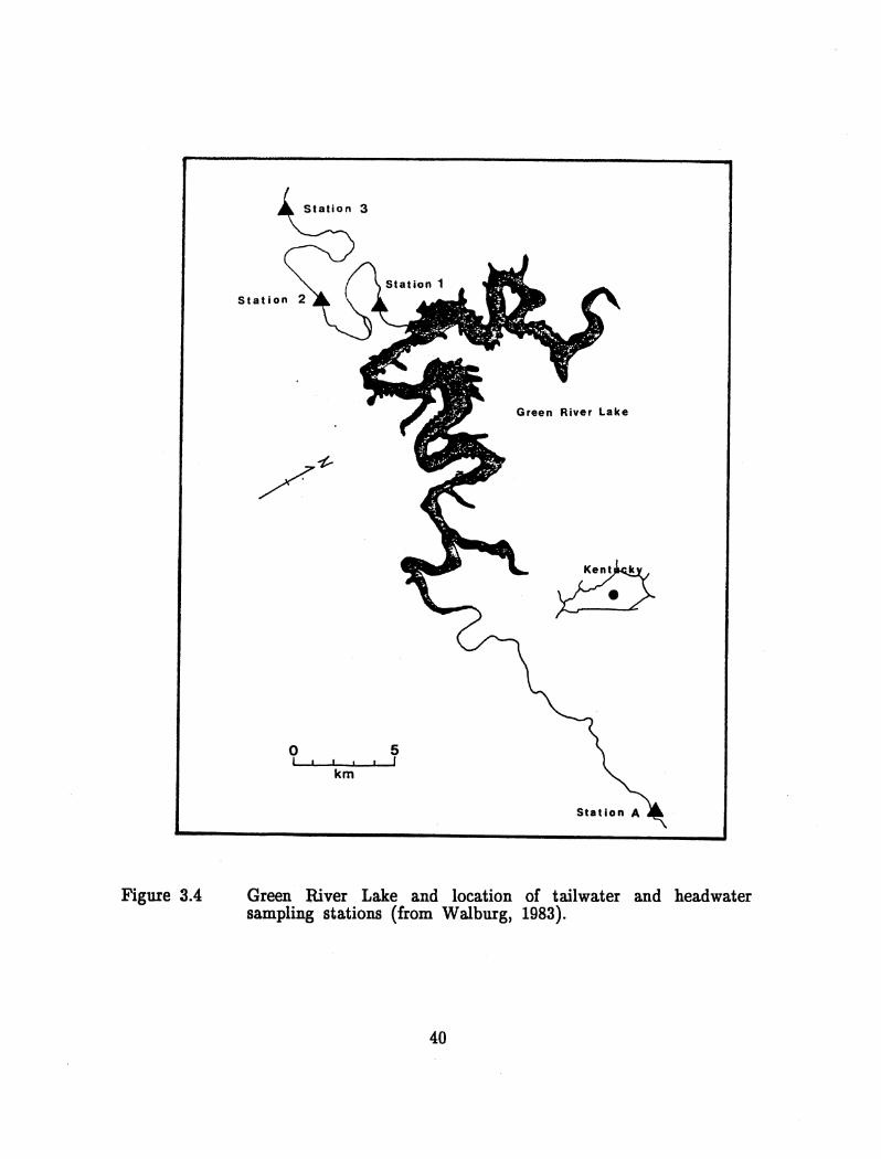
Figure 3.4
o I
km
5 I
Green River Lake
Green River Lake and location of tailwater and headwater sampling stations (from Walburg, 1983).
40

I ,
Beaver Lake
Figure 3.5
N
1
o I
km
Station 2
1 I
3
Location of samplin~ stations in tail water below Beaver Lake (from Walburg, 1983).
41

Figure 3.6
N
Hartwell Lake 1
~rOlina Ger:J
o 1.6 I I
km
Hartwell Lake and location of tailwater sampling stations (from Walburg, 1983).
42

o I
Figure 3.7
km
Lake Greeson
5 I
Station 1
Station 3
Lake Greeson and location of tailwater sampling stations (from Walburg, 1983).
43

bypasses located at two or nine different elevations. All four flood control projects had tailwaters with established minimum flows ranging from 0.8 to 2.4 m 3/s. The size substrate and topography of tailwaters below flood control projects differed from site to site. Detailed descriptions of the sampling station in each tail water and reservoir headwaters illustrate the differences in surface area, depth, substrate, and physiography (Tables 3.1 to 3.7).
Characteristics of the three peaking hydropower projects were generally similar, except for the relative size of the reservoirs and their discharge capacity. Water was discharged 20 to 40 meters below the reservoir surface, and release reflected demand for electricity, usually peaking during weekday, daylight hours. Detailed description of the sampling stations in these tail waters show differences in surface area, depth, and substrate.
Water quality samples were taken seasonally at all sample sites in 1979 and 1980 during low flow periods. Temperature and dissolved oxygen profiles were obtained for each reservoir to supplement tailwater quality data.
Several methods were used to collect macroinvertebrates because of differences in habitat among the seven tailwaters. All samples were taken during low flow periods.
3.3. Observations in Studies
3.3.1. Flood control projects
The physicochemical characteristics of Pine Creek and Gilham tailwaters were generally similar in 1979 and 1980. Summer water temperatures were high in both tailwaters (30 0 C in Pine Creek and 320 C in Gillham), and dissolved oxygen concentrations were generally above 5 mg/ l despite the withdrawal of water from anoxic areas of the reservoir. Conductivity, alkalinity and particulate matter were low in both tailwaters. Iron concentrations exceeded the EPA criteria for freshwater life (1.0 mg/ l) during late summer or fall in both tailwaters. Manganese concentrations in Pine Creek tailwater exceeded 1.0 mg/ l in late summer, whereas those in Gillham reservoirs never exceeded 0.4 mg/ i. The higher iron and manganese concentrations observed were presumably due to increased organic runoff, increased level of decomposition and extended anaerobic conditions in the reservoirs.
The warm water discharges produced a relatively dense macroinvertebrate fauna; densities and biomass of organisms were generally highest near the dams and decreased downstream, whereas diversities and numbers of taxa were lowest near the dams and increased downstream. Extended seasonal flood releases, together with increased levels of iron and manganese, may have limited benthic invertebrate diversities in the immediate tailwaters. The progressive increase in macroinvertebrate diversities at the downstream stations probably resulted from more variable habitat and/or moderation in the effects of flood releases.
44

~
Table 3~r
Description of SampJing Stations in the Tailwater Below
Pine Creek Lake, Oklahoma, and Type of Samples
Collected in 1979 and 1980 t Average
Distance Width x Bel1W Dam Length
Station ~kilometres2 {metresl
1 0.3 34 x 168
2t 2.1 55 x 624
3 12.1 23 x 336
Surface Area
!hectares2
0 .• 6
3.4
0.8
Average Depth, Maximum
Depth (metres)
0.3 O.S
1.0 2.0
1.2 1.6
*Measurements taken at minimum established discharge (1.8 ml/sec). **w - water quality. I - invertebrates .• F - fish. tInverte~rates were sampled at this station in 1979 only.
t (from Technical Report E-83-6)
Substrate (X Composition)
Silt 4% sand ·4% gravel 20% cobble 42% boulder 30%
Silt 11% sand 40% gravel 17% cobble 22% boulder 10%
Silt. 14% sand 31% gravel 32% cobble 16% bou1de-r 7%
Station Descri-ption
Shallow run with a riffle at the lower end of the station; no tree canopy or fallen timber. .
Wide pool with a run at upstream end and riffle at downstream end; extensive. tree ~anopy covers' both stream banks and fallen trees provide cover on the west bank.
Narrow pool with a run at upstream end and riffle at downstream end; extensive tree canopy covers the north stream bank and fallen trees provide cover on tbe south bank.
Type . of
Sample**
W. I
W, I. F
W. I. F

~ en
Table 3.2
Description of Sampling Stations in the Tailwater Below GUibam Lake, Arkansas, and Type of Samples Collected in 1979 and 1980 t
Average Distance Width x Below Dam Length
Sta~ ~kllometres) ~metres~
1 0.3 21 x 432
2t 4.0 46 x 244
3 15.3 36 x 360
Surface Area
~hectares)
0.9
1.1
1.4
Average Depth, MaximUIII
Depth (metres)
0.4 0.9
1.7 3.2
1.6 3.3
*Measurements taken at minimum established discharge (0.8 m3/sec). **W • water quality, I c invertebrates, F • fish. tInvertebrates were sampled at this station in 1979 only.
t (from Technical Report E-83-6)
Substrate (% Composition)
Gravel 40% cobble 55% boulder 5%
Silt 19% sand 39% gravel 23% cobble 9% boulder 10%
Sand l~% gravel 31% cobble 32% boulder 26%
Station Description
A run in a uniform channel with no tree canopy or fallen trees or large rocks for cover.
Deep, wide pool with a run and gravel bar at the upstream end and a wide shallow run at the downstream end; some tree canopy. boulders and fallen trees form cover.
Long pool with a run at the upstream end and a riffle at the downstream end; boulder-strewn banks provide cover and there is a large deep area in the pool.
Type of
Sample**
W, I
W, I, F
W, I, F

~
Table 3.3
Description of Sampling Stations in the Tailwater Below and Headwater
of Barren lliver Lake, Kentucky,
and Type of Samples Collected in 1979 and 1980 t
Station
1
2+
J
Aft
Distsnce Below Dam ~kl1om"tres2
2.4 in 1979 1.6 in 1980
7.2
21.1
3.4 above reservoir
AVl'rngc Width x Length ~metres)
37 x 354
37 x 335
21 x 465
14 x J59
Average Depth,
Surface Maximum Area Depth
~hect"res2 ~m"tres2
1.3 1.4 2.4
1.2 1.2 2.1
1.0 1.4 2.1
0.5 1.0 1.8
*Measurements taken at minimum established discharge (2.l m3!sec). **101 ~ water quality, I m invertebrates, F - fish. tOnly fish sample was taken at this station in 1980.
ttSampled only in 1980.
t (from Technical Report E-83-6)
Substrate (% Com~o!lition)
Silt) 30% sand) gravel 70%
Silt 50% gravel 50%
SUt 10% gravel) 73% cobble) boulder 17%
Sund 22% gravel 41% cobble ) 37% boulder)
Station Description
Primarily a large pool with a gravel shoal (water <1.0 metre deep) located in the center of the pool; 7 percent of the surface area has fallen trees, tree roots embedded in the bank, or undercut banks.
Primarily a wide pool with one riffle and one run located at the upstream end of the statIon; cover is primarily fallen trees.
Equal amounts of pool, run, and riffle with fallen trees and large rocks providing cover; several springs flow into the station on the north bank.
Approximlltuly cqulIl qUlIlltltlell o( pool., run, and riffle were present: cover pTovided by overhanging vegetation, boulders, and submerged logs.
Type of
Sample**
W, I, F
W, I, F
101, 1, F
II, I, F

~
~
1
2t
3
Att
Distance Below Dam (kllometres~
1.5
10.5
22.5
19.0 above reservoir
.-
Table 3.4
Description of" -Sampllng Stations iii the Tailwater and Headwa.1ier
of Green River Lake, Kentucky,
and Type of Samples Collected in 1979 and 1980 t .t'
Average Width x Surface Length Area (metres~ (hectares2
30 x 457 1.4
46 x 457 2.1
32 x 610 2.0
25 x 351 0.9
AveraRe Uepth, Maximum
Depth (metres)
0.6 1.8
1.2 2.1
0.9 1.8
0.8 1.1
Substrate (% Composition)
Gravel 60% cobble ) boulder) 40% bedrock)
Gravel 80% boulder) 20% bedrock)
Silt 10% gravel 70% cobble ) 20% boulder)
Sll,t 5% gravel 30% cobble 25% boulder) 40% bedrock)
Station DescriPtion
Approximately 40 percent of the station is shallow run «O.S metres deep) with several riffles; few pools are present, cover is provided by large rocks and boulders.
Most of the station is a long pool with a riffle at the downstream end; many fallen logs provide cover.
Diverse habitat with equal amounts of pool. riffle, and run with fallen trees, roots embedded in the banks, and large rocks providing cover.
Two large pools with one large run in· the center of the station; cover was provided by logs, overhanging trees and brush, end a few small boulders.
*Measurements taken at minimum established discharge (2.4 m3/sec). **w • water quality, I • invertebrates, F • fish. tSampled only in 1979.
ttSampled only in 1980.
t (from Technical Report E-83-6)
Type of
Sample**
W, I, F
W, I, F
W, I, F
W, I, F

~ CO
1'itlle 3.5
Description of Sampling Stations in the Tailwater Below
Beaver Lake, Arkansas, and Type of Samples Collected in 1979 and 1980 t
Average Distance Width x Surface Below Dam Length Area
Station {kilometres2 (metres2 ~hectares2
1 0.7
2 2.2 44 x 1800 7.9
3t 3.6 26 x 800 2.1
4 5.S 48 x 500 2.4
*Measurements taken at minimum flow (0.8 m3/sec). **W - water quality. I - invertebrates, F - fish. tFish were sampled at this station in 1979 only.
t (from Technical Report E-83-6)
Average Depth, Maximum
Depth Substrate (% {metres 2 ComEosition} Station Descri,2tion
0.4 Sand 3% Riffle. 1.0 gravel 88%
cobble 9%
1.5 Sand 4% Large pool with about 20 percent of 3.0 gravel 87% the area deeper than 2.0 metres.
cobble 9% Boulders strewn below limestone bluffs and some bedrock at upper end of station.
2.0 Approximately 30 percent of the pool 5.0 is deeper than 2.0 metres; some
boulders provide cover.
loS Sand 5% Approximately 20 percent of pool 4.0 gravel 88% deeper than 2.0 metres with cover
cobble 7% provided by submerged logs; some bedrock present.
Type of
Sample**
1
W, I, F
W. F
W. I. F

a1 0
Table 3.6
Description of Sampling Stations in the Tailwater Below Hartwell Lake, Georgia and South Carolina, and Type of Samples
Collected in 1979 and 1980 t
Average Distance Width x Surface lie low Dam Length Area
~ ~kUometres~ ~metres~ ~hectares2
1 1.0 61 x 392 2.4
2 4.0 68 x 382 2.6
3 12.1 62 x 481 3.0
*Heasurementl taken at minimum flow (3.0 m3/sec). **w • water quality, I • invertebrates, F • fish.
t (from Technical Report E-83-6)
Average Depth, Maximum
Depth Substrate (% ~metres2 Comj!0sition2 Station Descril!tion
0.9 Gravel 18% Lona .hallow pool with larlll rocks, 3.3 cobbla 6:t: boulder_, end a tow rnllon erGo ••
boulder 76% SI'urIlG vegstation, InDuLly bluu-greull or filamentous algae.
0.7 Sand 12% Lons ahallow pool with large rocks, 1.1 grava1 27% bou1dera, and a few fallen treea.
cobble 7% Sparae ve8etation, mOltly blue-8reen boulder S4% or filamentous alsae but some
Fontinalis ap. present.
0.7 Sand 23% LOnS ahallow pool with large rocks, 1.8 srava]: 25% boulderl, Ind I few fallen trees.
boulder 52% Splrse vegetation, mostly blue-sreen alsae and Podoltemum sp.
:,;
Type of
Saml!le**
W, I, F
W. I, F
W, I, F

at ....
Table 3.7
Description of Sampling Stations in the Tailwater Below
Lake Greeson, Arkansas, and Type of Samples Collected in 1979 t
Average D:lstance Width x Surface Below Dam Length Area
Station ~k!1ometres2 {metres~ ~hectares~
1 0.5 31 x 183 0.6
2 10.5 34 x 336 1.1
3 16.1 31 x 549 1.7
*Measurements taken at minimum flow (0.3 m3/sec). **w - water quality, I - invertebrates, po - fish.
t (from Technical Report E-83-{j)
Average Depth, Maximum
Depth Substrate (X ~metres~ . ComEosition2 Station DescriEtion
1.1 Silt 4% Upstream cnd ofpo01 has shallow run 2.8 sand 31% with bedrockbottolD and downstream end
gravel 30X deeper with boulders for cover; no cobble 22X fallen tilDber in water but there is an boulder l3X extensive streambank tree canopy.
1.7 Silt 3X Long relatively deep pool with a run 4.0 sand l6X upstream and a riffle downstream;
gravel 8X extensive tree canopy on both strealD-cobble 17% banks with fallentimber and boulders boulder 56% for cover.
1.S Silt 73X Long pool of which only the upstream 3.3 sand l5X hal.f was sampled and the upstream
gravel 8% boundrywasa riffle; extensive tree cobble 4% canopy on streambanks; some fallen
timber for cover.
Type of
Sample**
W, I, F
W, I, po
W, I, po

The fish communities of Pine Creek and Gillham tailwaters were similar in species composition and relative abundance. Sunfishes, suckers and catfish dominated the fish populations in both tailwaters, and fish were most abundant at the upriver station nearest the dam. Species composition was similar at upstream and downstream stations within the tailwaters but the relative abundance of some species varied by station.
Invertebrates in the immediate tailwaters were affected by the reservoir discharge, but those 12 to 15 km downstream had recovered and the species distribution reassembled that of a more natural stream community. In general, the relatively immobile invertebrate community appeared to be more sensitive to environmental changes caused by the dams than were fish populations. Fish were usually abundant at the station near the dams than downstream.
3.3.2 Cold-water release
The physiochemical characteristics of the tail waters below Barren River and Green River reservoirs were generally similar in 1979 and 1980.
Low water temperatures necessary for trout (~ 21 0 C) were marginally maintained in these tailwaters. Tailwater temperature immediately below the dams exceeded 21 0 C during most of the summer. Summer water temperatures in both tailwaters increased downstream as a result of solar warming. .
Dissolved oxygen levels were never less than 6.0 mg/ l in either tailwater in samples taken at minimum flow. Elevated levels of iron and manganese occurred periodically in both tailwaters in 1979 and 1980 because of release of water from the anoxic hypolimnion of the reservoirs. Weekly samples taken in the immediate tailwater of both dams during the summer of 1980 indicated that levels of ammonia, iron, and manganese were generally highest in October, but that elevations also occasionally occurred in August and September. Reasons for the fluctuations in concentration of iron, manganese, and ammonia are unknown but are probably related to reservoir biochemistry and reservoir operations.
Diversity and numbers of taxa were lowest near the dam and highest at the downstream station. Densities and biomass of organisms did not vary substantially among tailwater stations. Diversity and total numbers of taxa in the stream drift were higher above the reservoir than in the tailwaters.
The environmental differences at each station were also reflected in the taxonomic composition of the invertebrate communities. Downstream, the more diverse habitat and the gradual return to a more natural stream environment resulted in increased taxonomic diversity, decreased total numbers and a shift in the taxonomic composition.
The macroinvertebrate communities at the stations nearest the dams were apparently modified by environmental stress caused by reservoir discharge. In contrast, samples from above the reservoirs consistently inhibited the characteristics of natural stream communities. The tailwater stations farthest downstream were less affected than those near the dams,
52

which indicates some reduction in environmental stress. Species composition and relative abundance of fishes were similar in Barren and Green tailwaters. Population biomass in both tailwaters was dominated by rough fish (carp and suckers), populations of catchable sized game fish (black basses, rainbow trout and catfish) were small. Studies showed that reservoirs are the source of many fish found in tailwaters.
3.3.3 Hydropower Projects
Levels of discharge differed among the three hydropower reservoirs. Maximum r.eleases were about three times greater from Hartwell (750 m 3/S) than from Beaver (250 m3/s) and 10 times greater than from Greeson (75 m3/s). All three reservoirs were operated for peak powers.
Water temperatures were lowest at the upstream stations in Hartwell and Greeson tailwaters (never less than 21° C) and increased downstream. Maximum temperature in the shorter Beaver tailwater were much lower (12.2° C) and were generally similar at all three stations. Daily temperature fluctuatIOns of 2 to 6° C were recorded in Hartwell tailwater.
Dissolved oxygen concentrations were maintained above 5.0 mg/ l in Beaver and Greeson tailwaters, despite the deep reservoir withdrawal. Low dissolved oxygen « 5.0 mg/ l) recorded below Hartwell suggests that aquatic· life in this tailwater may be periodically stressed.
Variations in conductivity, pH, alkalinity and particulate matter were minor among tailwaters and were probably related to drainage basin differences. Iron and manganese concentrations in Hartwell and Greeson tailwaters were variable but highest levels occurred during fall months. High sulfides were maintained for prolonged periods.
The macroinvertebrate community at the sampling station nearest the dam in tailwaters of all three hydropower projects generally had the fewest taxa, lowest diversity and highest density. The dominant taxa at this station were similar in all three tailwaters.
The fish population in Greeson tailwater differed from those at Beaver and Hartwell. Distribution of fish differed in the tailwaters of the three hydropower projects. Stocked trout generally remained in the area where they were released and were not abundant at station 1 and least abundant at station 3 in all three tailwaters. Most sunfishes showed no location preference, abundance was similar at all stations within a tailwater. Several sucker species were more common at downstream stations than immediately below the dam.
In summary, the primary perturbation affecting the biota in tailwaters of the hydropower projects were the periodic water level and flow fluctuation and the generally low water temperatures. Low concentration of dissolved oxygen and high levels of iron, manganese and ammonia in release water may have stressed the organisms living in Hartwell and Greeson tailwaters, but the effects of these conditions could not be differentiated from those caused by flow fluctuations and temperature reduction. In beaver tailwater, the microinvertebrate and fish communities appeared to be stressed despite the
53

absence of high concentration of iron, manganese and ammonia and the presence of high levels of dissolved oxygen. The cold, fluctuating releases near the three dams appeared to limit both macroinvertebrate and fish fauna to organisms that were able to survive in these specialized environments.
3.4. Conclusions
The conclusions drawn from the studies are as follows:
( a) Elevated concentrations of iron, manganese, and ammonia were recorded below the six reservoirs that released anoxic water. The effects of these elevated concentrations on the tailwater invertebrate and fish communities were not determined.
(b) In tailwaters of the four flood-control projects, invertebrate drift at the sample station nearest the dam was dominated by Chaoboridae, a common reservoir inhabitant, other macroinvertebrates were few. Farther downstream, where tail water conditions more closely resembled those of natural streams, the abundance of Trichoptera, Ephemeroptera, and Plecoptera increased and that of Chaoboridae decreased.
(c) At both the flood-control and hydropower projects invertebrate diversities and numbers of taxa were generally lowest at the sample station nearest the dam where environmental stress was greatest.
(d) Numbers of benthic invertebrate species were highest in tail waters of flood control projects with warm water release and lowest in tail waters below the large hydropower projects.
(e) Trout stocked in tailwaters of hydropower and flood control projects with coldwater release moved little and generally congregated near where they were released; most were stocked near the dams.
(f) In the tailwaters of flood control projects, fish were most numerous at the station closest to the dam. In the tail waters of hydropower projects, warmwater species were generally more abundant downstream.
(g) Fish were most abundant in the tailwaters of the flood control projects and the small hydropower projects and least abundant in the tailwater of the large hydropower projects.
(h) Despite the occurrence of environmental stress caused by reservoir releases, all tailwaters in this study provided sport fishing.
(i) There was no clear relation between tailwater fish catch and reservoir discharge volumes.
(j) In-stream cover (e.g. boulders, fallen trees, backwaters) may have a moderating influence on the adverse effects of reservoir releases on tailwater biota.
54

(k) The distance below a dam necessary for a river to return to a natural environment was not determined from this study. Factors which determine downstream distance include time, volume, depth, and water quality of releases. Release effects can be modified by tributary inflow and by hydraulic factors within the stream such as pools, rimes, and substrate.
55

Chapter 4 Tailwater Quality Control
4.1. Introduction
Problems associated with the reservoir water quality and thereby affecting tailwater quality are as follows:
(i) degradation of potable water supplies.
(ii) limit or terminate recreation due to weed choked shallow areas and algal blooms.
(iii) low dissolved oxygen in deep waters and discharges.
(iv) accumulation of bottom sediments reducing storage capacity.
(v) increased turbidity and odor.
These problems arise due to anoxic hypolimnion, eutrophication and various physical and chemical processes. There are several techniques to control the quality of water in reservoirs and the tailwaters. These techniques have their advantages and disadvantages over each other depending upon the site specific conditions. These techniques are divided into four categories and described as follows:
1. Prereservoir treatment
2. Reservoir water quality control
3. Withdrawal control
4. Tailwater control
4.2. Prereservoir Treatment
4.2.1. Siltation basins
A siltation basin is used to detain incoming water long enough to allow significant deposition of nutrients and particulate matter. Water that flows to the main reservoir should have greatly increased quality as a result, while materials deposited in the siltation basin can be periodically dredged. The design of the siltation basin will be site specific depending on the rates of water, nutrient, and silt income. A critical problem with the use of this system is obtaining the area needed to construct them. If a portion of the upper reservoir is modified to form a smaller reservoir, then significant loss of
56

storage capacity may occur. The siltation basin may require substantial maintenance in the form of harvesting of plants and the removal of accumulated silt through dredging. This method may prove to be highly effective. The cost depends on the site specifications. It is not applicable to high volume, hydropower reservoirs as to smaller recreational and potable water supply reservoirs.
4.3. Reservoir Water Quality Control
4.3.1. Phosphorus inactivation
Phosphorus inactivation is carried out through the addition of aluminum sulfate or sodium aluminate (or both) to the lake or reservoir. Aluminum has been the element of choice rather than iron because the complexes and polymers that form after the addition of either of these aluminum compounds are apparently inert to changes in oxidation-reduction potential, such as would occur during the development of hypolimnetic anoxia. Phosphorus will remain bound to these complexes, where as iron will release phosphorus as the redox potential falls.
Aluminum sulfate or sodium aluminate will produce the formation of aluminum hydroxide in water with carbonate alkalinity. This hydroxide is a visible floc or precipitate that is very absorptive of phosphorus and will not release it under conditions of low dissolved oxygen. The maximum dose of aluminum sulfate that can be added depends upon the initial alkalinity of the reservoir and hence is unique to each reservoir. This method is highly effective and the longevity is up to 12 years. The potential for serious negative impacts from low pH or the toxic effects of dissolved aluminum exists with the addition of an aluminum salt to a reservoir. This method is labor intensive.
4.3.2. Dilution and flushing
Dilution is a procedure in which water of low nutrient content is added for the purpose of lowering the reservoir'S concentration of nutrients to a level at which algal cell growth is limited and cell washout increases. Flushing emphasizes cell washout through a sharp increase in the water exchange rate. The inflowing water may not necessarily have a lower nutrient concentration.
Both techniques can produce large improvements in trophic states and are highly effective. These methods require continual water input during the growing season. The primary drawback is the availability of the additional water and possible effects of increased reservoir discharge on downstream areas.
57

4.3.3. Sediment removal
. Sediment removal is used for deepening and to remove nutrient rich or contaminated sediments and to control macrophyte infestations. The object is to regain lost storage capacity and to improve water quality by control of internal nutrient release. The sediments are removed using the dredges. The two categories of dredges are mechanical and hydraulic.
Sediment removal is one of the most effective and commonly used methods of improving reservoirs. It is highly effective and the longevity is years if the reservoir is dredged deeply and the sediment income is controlled. Several undesirable effects can be observed at the dredging site which include creation of plumes of turbid water, liberation of nutrients, destruction of benthic organisms and the release of toxic substances. In reservoir disposal many result in burial of organisms and the creation of new and less desirable substrates. Upland disposal can create nuisance conditions for nearby residents, contaminate groundwater and discharge toxins into the drainage water. Sediment removal projects require careful planning, design and construction since the cost may be considerable and there i~ potential for negative environmental impacts.
4.3.4. Hypolimnetic aeration
The purpose of hypolimnetic aeration is to increase the dissolved oxygen concentration in the hypolimnion without causing thermal destratification. The hypolimnetic aeration systems can be grouped into three types: 1) mechanical agitation, 2) air injection, and 3) oxygen injection.
In a mechanical agitation system, water is pumped from the hypolimnion to a splash basin or shore, where it is aerated and then returned to the hypolimnion. The air injection systems are divided into two types, the partial air lift and the full air lift designs. In the partial air lift system, compressed air is injected at the bottom of the unit, but the air-water mixture does not rise to the surface. Instead, the air and water are separated at depth so that the air is routed to the surface and the aerated water is returned to the hypolimnion. This type of design is illustrated in Figure 4.1. In full air lift systems, compressed air is injected at the bottom of the unit, as in the partial air lift, but the air-water mixture rises to the reservoir surface where the air is released to the atmosphere and the water is returned to the hypolimnion. This system is illustrated in figure 4.2. In liquid oxygen systems, the water is withdrawn from the hypolimnion. After passing through a shore based pump on its way back to the hypolimnion, pure oxygen is injected within the piping system. This design is called side stream pumping. Another type of oxygen injection involves pumping gaseous oxygen into the hypolimnion through diffusers. This system is depicted in figure 4.3.
Prior to the selection of the aeration system, the following data must be obtained:
58
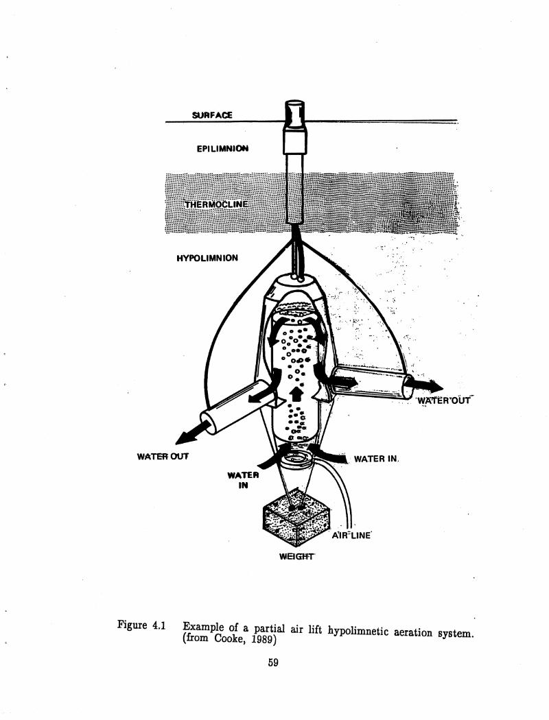
SURFACE
EPILIMNION
~ .~. "
HVPOLIMNION
... ,0,' ...
WATER OUT
Figure 4.1 Example of a partial air lift hypolimnetic aeration system. (from Cooke, 1989)
59

WOOD DECK
EPILIMNION
HYPOLIMNION
Figure 4.2
+
o 0 o
0 00 0 00 0
00 0 o 0
0 0 000
. ~""-~""'" INJECTION
WATER fN
Example of a full air lift hypolimnetic aeration. (from Cooke, 1989)
60

10 15 20
TEMPERATURE. -c 10
o r---------~----~~~~ __
10
E 20 ~ Ii: '" c
30
.
15
, , a a a I I I I I
. :
/~ , ~
~ ,
~
20
~
, ~ ,
o 2 4 e a 10 0 2 4 • 8 10 DISSOLVED OXYGBt" ...,.
a. Exaple profiles of di8Ml~ ..,pn aDd te.perab1re with (left) 8Jld without (rtaht) oxygenation
EVAPORATOR
SURFACE .. . .. "" .. .. . ..
• ••• co # • " . ... . . ... .
DIFFUSER·
Figure 4.3 Oxygenation through diffusers (from Cooke, 1989).
61

(a) determination of the hypolimnetic volume to be aerated,
(b) determination of the hypolimnetic oxygen depletion rate,
(c) determination of the amount of oxygen needed.
This method is highly effective in increasing dissolved oxygen. The hypolimnion remains aerobic as long as aerators operate. The full air lift system appears to be least costly and most efficient, with fewer negative environmental impacts. Problems with hypolimnetic aerators include undersizing, unintentional destratification and creation of a metalimnetic oxygen minimum.
4.3.5. Artificial circulation
Artificial circulation is a procedure to destratify a reservoir to create isothermal and isochemical conditions through the mixing action of compressed air or pumped water. The devices used are the air lift pumps, mechanical pumps and water jet systems. Air lift, or pneumatic diffusers, employ air injection into a pipe laid along the sediment surface. Hydraulic destratification uses a pump intake diffuser system to create high momentum buoyant jets that induce a great deal of mixing. Water is withdrawn from the epilimnion and pumped through a diffuser in the hypolimnion. Hydraulic destratification is believed to be more efficient than pneumatic destratification. This technique has been very successful in increasing dissolved oxygen and decreasing the concentrations of iron and manganese. Improvements continue as long as the circulation device is operated. Long-term effects are unknown. The cost is comparatively low.
4.3.6. Water level drawdown
Water level drawdown is a multipurpose reservoir improvement technique. It is used to control some nuisance plants, to provide access to dams, docks, and shorelines for repair and installation purposes, for fish management, for sediment consolidation and removal, and for installation of sediment covers. Control is achieved through drying and freezing for a period sufficient to destroy the thallus, roots and rhizomes and perhaps some reproductive structures.
The feasibility of this method for a particular reservoir is dictated largely by its use. Long-term drawdown could not be used in a hydropower reservoir, whereas flood control reservoirs are good for water level drawdowns, particularly during winter. This technique is usually effective for at least one year. Negative aspects of this method primarily involve problems of access to water by reservoir users, failure to refill, and possible effects on fisheries. The cost involved is minimal.
62

4.3.7. Harvesting
Harvesting is a procedure by which aquatic plants are cut, collected and removed from the water. This technique can bring about some control of plant regrowth, open the infested area to reaeration, lower the amount of organic matter in the water column or deposited on sediments and may contribute to improvement in water quality through the removal of nutrients and organic matter. Most harvesters are single-stage machines that cut the vegetation with one horizontal and two vertical sickle-blade cutter bars, store the collected plants on board via a conveyor from the cutterhead to a storage compartment, and unload the plants at shore via additional conveyors.
This method is moderately effective and the longevity may range from weeks to months. Negative impacts are minor-like turbidity and occasional algal blooms. The initial equipment costs are high and the operator, storage, and maintenance costs may be high.
4.3.8. Biological controls
The biological control of nuisance macrophytes and algae is potentially the most effective method in terms of costs and long-term control. However, the present day knowledge of how to use biological controls is not well developed. Biological control is employed to obtain an acceptable level· 'Of plant biomass through the introduction of species that graze or parasitize specific plants or by the manipulation or elimination of endemic animal species that directly or indirectly control plant growth. The use of biological controls can produce a slow, gradual response that may be long lasting in contrast to other methods. An example is grass carp which are the voracious consumers of aquatic plants. These animals can approach the 'ideal' biocontrol agents when the system to be treated is large. It involves very low initial and long-term costs, low maintenance cost and long-term effectiveness. Some insects and pathogens are also used as biocontrol agents of nuisance exotic vegetation.
Biomanipulation is a term used for methods to control algal biomass. Among them is the manipulation or management of food webs to control fish species that recycle nutrients during growing and feeding, or that promote algal growth through their predatory activitieS on microscopic animals (zoo plankton) which graze on algae. Fig. 4.4 illustrates the open-water food chain or web. Zooplanktivorous fish (e.g. gizzard shad, small sunfish) graze on the largest species of zooplankton. These zooplanktons are the most efficient grazers of algae, and their abundance eliminates a significant source of mortality to algae. Any factor that produces significant and prolonged zooplankton mortality may bring about persistent algal blooms, low transparency and associated problems with dissolved oxygen and quality of potable water. Restructuring of fish communities offers great promise for algal control but may be impracticable for large reservoirs.
63

.. .. ~ .. ~.... .: -.. ~ . . . ~ .. .. 'I\f:~ .~ ..
Jy •• ~. ~o· .: ?1' ~ ;7t.. . .. , '.~ .. ~ . . .... ~
NUTRIENTS
PISCIVOROUS FISH
I EAT ,
PLANKTIVOROUS Fat
I EAT ,
HERBIVORES
I EAT , .
ALGAE
I USE
t NUTRIENTS ,
RECYCLE
I BENTHIVOROUS
FISH
Figure 4.4 The aquatic food chain. (from Cooke, 1989)
64

4.3.9. Sediment covers
Sediment covers are used to control or eliminate nuisance rooted plant growth, particularly in limited areas of reservoirs such as cover, marinas, swim beaches and boat docks. Some covering materials are actually screenlike in nature so that gas bubbles do not accumulate under them. Three materials, aquascreen (fiberglass), Dartek (nylon), and Typar (polypropylene) have been shown to be effective. The longevity ranges from months to years. The installation may be difficult and costly. The screens may float to the surface and clog intake structures.
4.3.10. Herbicides and algicides
Herbicides and algicides are applied either as liquids or granules to nuisance plant populations at concentrations known to be sufficient to produce elimination or control of biomass, usually through interference with plant cell metabolism. In some instances, chemicals are used together for controlling macrophyte and algal problems simultaneously, or chemicals may be used in conjunction with other procedures such as harvesting, grass carp or insects. Copper has been used as an algicide to produce short-term relief from nuisance algal blooms. The use of copper results in several significant environmental impacts. A massive algal kill may produce a large decline in epilimnetic dissolved oxygen as the cells decay. Hypolimnetic dissolved oxygen may fall sharply. Copper is a highly toxic metal to animal groups particularly some fishlike salmonide and walleye. Ingestion of copper in potable water apparently will not produce copper toxicosis in humans.
Diqual is known to be an effective herbicide. Its mode of operation is to inhibit photosynthesis and stimulate respiration. Endothall acts on plant tissues to produce abnormal permeability, loss of water and wilting. susceptible plants may be controlled for weeks to months. Another herbicide 2,4-D is a phenoxyacetic acid. Another herbicide known as Fluxidene is a slow acting, rapidly degradable that is very effective against a broad spectrum of submersed and emergent aquatic plants.
Costs of herbicide treatments range widely. Plant density, area to be treated, types of plants, and other factors will influence cost greatly. Algicides are effective for days whereas herbicides provide at least seasonal control. Some chemicals are toxic to fish and fish food organisms. Long-term effects on ecosystems are unclear.
65

Operational and structural water quality enhancement techniques
4.3.11. Guide curve change
Many reservoir projects operate under some type of water control plan that relies on seasonal change of reservoir elevations. This sequence of reservoir elevation change is usually termed a guide curve. Modification of the guide curve is a technique that relies on changing the hydraulic residence time of inflow in the pool to control poor quality inflows. This can be accomplished by maintaining a small pool through most of the flood control season and allowing undesirable inflows entering the reservoir to be flushed through. The reservoir is then allowed to fill to summer pool elevation later in the season, when the inflow water quality is typically better. Figure 4.5 shows the example of guide curve modification.
By modifying the hydraulic residence time of the reservoir, undesirable inflows can be routed through the reservoir or retained to allow sedimentation to occur. This technique is highly effective on small to medium sized reservoirs. The longevity is seasonal and cost is minimal.
4.3.12 Inflow routing
Inflows to reservoirs can create problems with reservoir water quality. If the inflow is poor, containing high concentration of nutrients, suspended solids or other undesirable constituents, poor reservoir quality may result. Routing of inflow is a technique based on the water control operation or plan for the reservoir. Undesirable inflows are identified and routed through the reservoir to minimize impacts to the existing reservoir water quality, similar to routing of flood flows through a basin. Selective withdrawal capability greatly enhances this technique if the inflow occurs at some intermediate depth. Figure 4.6 shows the routing of undesirable inflows.
The effectiveness of this technique depends on reservoir size, distance of inflows to outlet works and strength of density difference between inflow and reservoir. The longevity ranges from days to months. The cost is minimal to none.
4.3.13. Supplemental releases for water quality
This method relies on selective withdrawal techniques to modify the water quality of the reservoir or its release. It relies on evaluating all of the release structures at a given project and determining whether it is possible to meet the water quality goals by operating a combination of structures even though they may not be intended for this purpose. For example, during the stratification season, release structures that withdraw hypolimnetic water may degrade reservoir releases because of significant concentration of iron, manganese and hydrogen sulfide. An operational technique that may be used to enhance the release quality is to release water from the epilimnion through a spillway gate, or if the elevation of the flood control intake is the same as that for hydropower to release through a flood control gate to increase
66

1,160 r-----.----r-~-""T"""-_r__-r__,-__r-_r-_,__-_r__,
lLL.
1,140
~ 1,120
~ > ~ 1,100 w II:: (5 i 1,080
w II:: 1,060
1,0400
Figure 4.5
2 3
,," ,," ,
,,' "
,,' ,
5 6 7 MONTHS
" , , , , /~ IJODIFICATION
8 9
Example of grid curve modification. (from Price et al., 1992)
67
12

~VEIJJCIIY PROFILES
Figure 4.6
TEMPERATURE
Routing of undesirable inflows. (from Price et ai .. 1992)
68

reaeration through the flood control outlet and stilling basin. Figure 4.7 illustrates the improved dissolved oxygen with supplemental releases.
The effectiveness of the technique depends upon the location and elevation of intake of release structures. The negative feature is release of additional water.
4.3.14. Concentration of flow through one gate
The operation of water control structures with multiple horizontal gates usually requires that all gates be operated the same for a given release condition to achieve as even a flow distribution downstream as possible to prevent scour and erosion to the stilling basin and downstream. A modification to the gate operation during low flow periods to increase the unit discharge may be used to enhance the dissolved oxygen by concentrating the flow, which normally would pass through all gates to pass through a minimum number of gates. This would increase turbulence in the stilling basin and enhance reaeration. Figure 4.8 shows the effect of flow concentration through a single gate.
The effectiveness of this technique is moderate. The cost involved is minimal. The negative features are possible increased scour and erosion of stilling basin and downstream.
4.4. Withdrawal Control
4.4.1. Hypolimnetic withdrawal
In many reservoirs and lakes, thermal stratification during summer isolates the hypolimnion from the surface layers, which results in development of anoxic conditions in the hypolimnion. The anoxic condition allows phosphorus from internal sinks to be released to the hypolimnion and ultimately contributes to the eutrophication of the lake. Selective evacuation of the hypolimnion, termed hypolimnetic withdrawal, can be used to remove excess phosphorus concentrations from the intake and to reduce the eutrophication. Figure 4.9 shows a schematic of the hypolimnetic withdrawal. Epilimnetic water, which maintains adequate concentrations of dissolved oxygen, is retained in the lake.
The effectiveness of this method depends on the lake volume. Usually this method is effective on small lakes with strong stratification. The negative aspect is removal of the hypolimnetic zone and will reduce or eliminate habitat for cold water fisheries. Downstream release will typically be of poor quality. The cost is minimal.
69

Figure 4.7
6~----~----~------~-----r-----'
5
...J
~ 4 :::t
o o a::: 3 w ~ ~
~ 2 to-
SUPPLEMENlAL FLOOD CONTROL
OL-----~----~------~----~----~ JUN JUL AUG SEP OCT NOV
Example of improved dissolved oxygen with supplemental releases. (from Price et al., 1992)
70

Figure 4.8
6~----~------~-----.,-----~
LEGEND 5 c:=J 2 GATES, HT OPENING
~ 1 GATE. 2-FT OPENING ~ , (OTHER CLOSED) g 4 .................. ~
o c ~ 3 w !;( 3: 'i. 2 I-
oL---~ __ --L-__ ~ __ ~~~~ __ ~
o 2
Example of flow concentration through a single gate. (from Price et al., 1992)
71

NUTRIENTS CXJ TEUPERATURE - - -
NUTRIENTS CXJ TEUPERATURE - - -
Figure 4.9 Nutrient reduction through hypolimnetic withdrawal. (from Price et al., 1992)
72

4.4.2. Underwater dam
Reservoirs that exhibit strong thermal stratification with a cool hypolimnion throughout the summer months may be able to maintain a cool-water fishery in the hypolimnion. Reservoirs that operate a bottom withdrawal structure, such as a hydropower project, deplete the cool hypolimnetic water during the summer months. One alternative to releasing the hypolimnion is to install a submerged barrier curtain or dam on a portion of the reservoir to retain the cool water during the summer by preventing its release downstream. This technique would prevent movement of the hypolimnion and effectively create a trap in the reservoir for cool water. Figure 4.10 shows the schematic of a submerged dam. This relatively new technique has been implemented in only one project, Cherokee Reservoir, and found to be successful. However, an oxygenation system was required to be installed to maintain DO levels for survival of cool water species.
The negative features are that sediment trap and may require an conditions in the underwater refuge. high.
4.4.3. Turbine venting
the underwater dam may act as a aeration system to prevent anoxic The costs involved are moderate to
The release of water with low dissolved oxygen is the result of hypolimnetic withdrawal of water low in dissolved oxygen during hydropower generation in the stratified periods. As the flow passes through the turbines, conditions become very favorable for reaeration to occur. However, reaeration does not occur at this point because of the lack of a source of oxygen. Turbine venting is a technique that allows oxygen to enter the draft tube downstream of the turbine and increase the dissolved oxygen in the release water. The low pressure in this region is controlled by the geometry of the turbine and draft tube, flow rate, operating conditions, headwater, and tailwater elevations. This low pressure controls the air flow rate into the draft tube. Once this introduced air is entrained into the flow in the draft tube, the hydrostatic pressure increases with the movement down the draft tube and in turn increases the oxygen transfer efficiency over that normally occurring at the surface. Figure 4.11 depicts the vacuum-breaker venting system.
Field applications show that a maximum of 30% of the oxygen deficit in the release can be satisfied by turbine venting where some loss in generation efficiency of the order of 3% can be anticipated with the addition of air. The costs involved are moderate to high depending on the require modification to the turbine.
4.4.4. Submerged skimming weir
The thermal stratification that occurs at most reservoirs can create problems with release water quality. If the intake structure withdraws waters from the hypolimnion, the release may be low in dissolved oxygen or contain high concentration of undesirable trace constituents. In this case, withdrawal
73

UNDERWATER DNI
EUBAYUENT
liNN 8OlJ( OF RESERVOIR ..
Figure 4.10 Schematic of submerged dam. (from Price et al., 1992)
74

.', v .
'04 ' '" 4
,,'
.' v ,'04 ' ' ',4
,,' .~
'0(\
v'
v .~
. '. "
TURBINE SHAFT
AIR-WATER MIXTURE
',.. :.' "v, VJCUUIJ- , '.' BREAKER . AlR SUPPLY
VALVE· PIPE •
. v • ~ . 9 .•
". " i> .
v .
,,'
.. SCROLl CASE
Figure 4.11 Vacuum breaking venting system. (from Price et al., 1992)
75

of water primarily from the epilimnion may be desirable. To increase the amount of epilimnetic water in large release, a submerged skimming weir can be designed and installed. This structure is designed to extend to the top of the reservoir thermocline and prevent the withdrawal of the hypolimnion. A numerical model can be used to simulate various stratification patterns and discharges and to determine the optimum crest elevation for the weir. Figure 4.12 shows the schematic of the submerged skimming weir.
Several projects for which weirs have been evaluated showed that the water quality was improved. This technique is effective at given flow rates. The construction of skimming weir is expensive.
4.4.5. Multilevel selective withdrawal
The operation of a multilevel intake structure requires the consideration of numerous project conditions and constraints, the most important of which is thermal stratification. As stratification develops, the limits of withdrawal for a given port are reduced because of the density differences imported by the thermal stratification. Thus, flow through a pool at a given elevation may not result in a release temperature similar to that observed at the centerline elevation of the port or that desired to meet a . downstream objective. Selective withdrawal is a technique used to identify the withdrawal zone for a given structure. The theory is based on identification of the density impacted withdrawal pattern.
This technique is very effective and lasts for years or the life of the project, but is expensive.
4.4.6. Localized mixing
The thermal stratification can create problems with release water quali ty. If the hypolimnion becomes isolated from the surface and turns anoxic, reducing conditions for iron, manganese and hydrogen sulfide will prevail. Localized mixing is a technique that provides enough mixing in a local area to reduce the thermal stratification. This is usually accomplished by pumping surface water down into the hypolimnion to achieve a locally uniform vertical temperature profile. The jet from the pump provides the energy needed to disrupt the stratification and causes entrainment of the epilimnetic waters in the release discharge to enhance the water quality. Figure 4.13 illustrates the schematic of localized mixing.
Application of localized mixing has been tested in a number of locations with axial flow and direct-drive mixers and found to be successful to reservoirs without selective withdrawal structures. The costs involved are moderate.
76

RESERVOIR
TEMP. TEMP.
Figure 4.12 Schematic of submerged skimming weir. (from Pri!!e et aI., 1992)
77
- -- - --- -- -- --- - --------_._------ ------ -- ---------~------- - ~-

TEMPERATURE PROFILE
Figure 4.13 Schematic of localized mixing. (from Price et ai., 1992)
78

Chapter 5. Tailwater Quality Modeling
5.1. Introduction
. Thermal stratification in reservoirs is accompanied by depletion of dissolved oxygen (DO) in the bottom waters (hypolimnion). Oxygen
. depletion and the establishment of reducing conditions in the hypolimnion increase mobilization from. the sediments of dissolved nutrients (i.e. ammonium and phosphorus), sulfide, reduced metals (e.g. iron and manganese) and organic substances. These substances can accumulate in the hypolimnion, impacting the in-pool and release water quality. Reservoir releases that are low in DO and high in reduced substances can threaten aquatic life and cause water treatment problems for downstream water supply.
When water is released downstream, stream reaeration occurs and reduced substances begin to oxidize. Water quality improves as the water, moves downstream and eventually recovering to a more natural stream condition. A better understanding of the recovery mechanisms is needed to better manage tailwater quality problems.
5.2. Approach of Study
Effective water quality management of reservoir tailwaters requires assessment of existing conditions and prediction. of future conditio.ns r. esulting from structural and/or operational modifications of the dam or tailwater system. For example,· the conversion of a nonhydropower, deep release to a hydropower release can lead to water quality problems.
Mathematical water quality modeling is a cost-effective tool for predicting future conditions resulting from human actions. A model can be used to estimate downstream wate.r quality for a proposed release condition at a dam. However, water quality models are limited in the context of process description. For example, first order decay can be expressed mathematically as
dC at = - KC (5.1)
This equation has been used to describe the kinetics of numerous water quality constituents. The difficulty in applying this equation is to estimate or calibrate the reaction coefficient K. Empirical observations are required to develop K values for site specific conditions.
79

5.3. Tailwater Quality Processes
The mathematical model for water quality of reservoir tailwaters is based on the one-dimensional (l-D) mass conservation equation for streams
where
8C [ ac ] [ 82C ] or + u Ox = D 7JX'I"
U = stream mean· velocity
x = distance downstream
D - longitudinal dispersion
:I: S
s - rate of change in concentration resulting
from transformation or chemical reactions
(5.2)
The above equation assumes completely mixed conditions over the depth and width of the stream. The dispersion term, which is the first term on the right side of the equation, is usually much less than advection. Neglecting dispersion, assuming steady-state conditions, eq. 5.2 simplifies to,
dC at = :I: S (5.3)
If s in eq. 5.3 is a first order loss rate (i.e. KC) then eq. 5.3 is identical to eq. 5.1.
5.3.1. Manganese
Anoxic conditions in the hypolimnion of deep reservoirs induce the formation of dissolved, reduced manganese, Mn +2. Reduced manganese accumulate in the reservoir, affecting in-pool as well as release water quality. Mn +2 accumulates in the water column under anoxic conditions. The oxidation of reduced manganes~ in the tailwater can be influenced by many environmental facts such as temperature, pH, presence of DO, degree of mixing etc. The removal of reduced Mn +2 from reservoir tail waters can involve physical processes (e.g. adsorption) as well as oxidation. The Hess model for manganese reaction is used in the tailwater quality model, which states
d[Mn(II)] dt = - [Ko[OH-)2(DO) + K(OH-)2(DO)(MnIV)] (MnII) (5.9)
80

where
Mn(II) = dissolved (reduced manganese concentration, moles/ l), Ko = homogeneous reaction rate, day~~moles/l),
[OR] = hydroxide ion concentrations, moles/i,
[DO] = dissolved oxygen concentration, moles/ l, K = heterogeneous reaction rate, day~l(moles/l),
Mn(IV) = oxidized manganese concentration, moles, l
5.3.2. hon
The rate of oxidation of reduced iron (Fe++) is first-order with respect to concentration of Fe++ and 02 and increase second order with respect to the H+ concentration. This rate law is expressed as
d(Fe(II)) = _ k [Fe(II )][DO] dt Fe [H+]2
where
Fe(II) = concentration in modes/ l of ferrous iron, and
kFe = 3.0xlO~12 moles/l min~1 at 20· C
(5.5)
Eq. 5.5 is in the form of eq. 5.1 with the overall reaction rate for ferrous iron described as
K = k [DO] Fe Fe [H +]2
As reducing conditions progress in anoxic reservoir bottom sediments, sulfate reduction follows iron reduction and iron sulfide forms. Iron sulfide may be temporarily suspended in the water column and released to the tailwater.
81

5.3.3. Sulfide
Dissolved sulfide can exist as hydrogen sulfide (H2S) bisulfate ion (HS-). At a pH of 7, sulfide exists as about half hydrogen sulfide and half bisulfate ion. Oxidation kinetics of sulfide in natural waters is very complex an~ poorly understood. The oxidation of sulfide can be described as first order with respect to HS- with a rate that increases with increasing temperature, pH and concentrations of DO, metal ions and initial sulfide. The oxidation rate of sulfide is strongly dependent on pH. The reaction can be described by the Michaelis-Menton law as follows:
where
dS DO Of = - Ks S .... D"'"'O,....:;.t----:-+~D""'O~
s = sulfide concentration in the form of HS -, mgt i, Ks = sulfide oxidation rate, day-i,
DO - dissolved oxygen concentration, mgt i, DO t = dissolved oxygen half-saturation constant, mg/l
The sulfide oxidation rate approximately doubles for 15° C temperature increase. This dependency on temperature can be represented as
where (Ks)20 = the oxidation rate at 20" C.
5.3.4.. Other water quality constituents
Other water quality constituents that are of primary interest in reservoir tailwaters are temperature, dissolved oxygen and nutrients. Heat exchange mechanisms are relatively well understood and the capability to accurately model stream temperature is well established. Dissolved oxygen is required for aquatic life and is of prime importance in reservoir tail water and the source and sinks of oxygen must be considered. The nutrients nitrogen and phosphorus can exist in various forms: organic, inorganic, particulate and dissolved. The only nutrient form that presents an immediate potential problem in tailwaters dominated by anoxic hypolimnetic releases is ammonium.
Oxidation of reduced substances in the tailwater is a major sink of oxy~en. The primary source of oxygen is stream aeration. The oxidation of MntII) may be represented by
82

2Mn+2 + 02 + 10 H20 o-i 4 Fe(OH)3 + 8H+
This reaction requires 0.14 mgt l of DO to oxidb;e 1 mgll of Fe(II).
Oxidation of sulfide can produce sulfur (S), thiosulfate (S 0-2 ), sulfite 3 3
(SO-2) or sulfate (SO ... 2) according to the following reactions. 3 4
HS" + i 02 + H + o-i H20 + S
HS- + 202 o-i SO-2 + H+ 4
The above reactions require 0.5, 1.0, 1.5 and 2,0 mgt l DO per 1.0 mgt l of S-2.
Ammonium can exist in un-ionized form NH3 or in ionized form NH4+ (ammonium). Nitrifying bacteria convert ammonium (NH4+) to nitrate (N03-) where :the overall reaction is described as
NH4+ + 202 o-i N03- + H20 + 2H+
Thus requiring 4.57 mgt l 02 per 1.0 mgt l ammonium nitrogen.
The rate of nitrification, or the oxidation of ammonium, can vary widely and is dependent on temperature, DO, pH and stream hydraulics. Nitrification isa source for nitrate nitrogen and denitrification and algal uptakes are sinks.
Sediment oxygen demand (SOD) can have a significant impact on DO in surface waters. SOD values of 1.0· to 2.0 g/m2/day were measured in the Nimrod and Rough river tailwaters where the bed consisted predominantly of fine sediments. These rates exert an oxygen demand that is comparable to the demands caused by oxidation of reduced substances and are the same order of magnitude as reaeration for sluggish streams~ Therefore, SOD should be considered for a tailwater DO model.
Reaeration is considered to be the primary source of DO in reservoir tailwaters fed by deep releases because production of oxygen through photosynthesis decreases with temperature and deep releases tend to be cold.
83

5.4. Numerical Model
The focus of the tailwater quality numerical model (TWQM) is to predict the downstream transformation of problem constituents, such as DO and several of the reduced substances (Le. iron, manganese, sulfide and ammonia). The model is one dimensional in the streamwise direction. TWQM does not allow time varying flow or water quality inputs, and a steady-state solution is performed.
TWQM is based on the U.S. Environmental Protection Agency (EPA) 1-D stream water quality model, QAUL2E. The major modification to QUAL2E was to include subroutines to model the reduced substances in tailwaters. In addition to the QUAL2E-based tailwater component, there is a reservoir release component. Reservoir release water quality is required for the upstream boundary condition of stream components. The. user may specify this information from observations or can predict the release concentrations based upon observed in-pool concentrations using the SELECT model. Given the in-pool temperature stratification, the outlet features, release flow rate and vertical distribution of water quality constituents, SELECT computes the release concentrations. SELECT also includes the structural aeration component that predicts uptake of dissolved oxygen as flow passes through the release structure. The. combination of SELECT with the tailwater model allows the user to evaluate the impact on downstream water quality of various release schemes, such as hydropower retrofit or moving the vertical location of the intakes of the outlet structure. TWQM has the capability of simulating up to 17 water quality constituents as follows:
1. Dissolved oxygen (DO) 2. CBOD
3. Temperature
4. Algae as chlorophyll-a
5. Total organic nitrogen
6. Ammonia nitrogen
7. Nitrite and nitrate nitrogen
8. Total organic phosphorus
9. Dissolved inorganic (orthophosphate) phosphorus
10. Dissolved (reduced) iron
11. Dissolved (reduced) manganese
12. Total dissolved sulfide
13. Iron sulfide
14. Arbitrary nonconservative constituent
15. Two conservative constituents.
84

Figure 5.1 illustrates the various state variables and how they interact. The model solves the steady-state mass balance equation (Le. mass transport equation or advection-diffusion equation with mass sources/sinks) for each state variable.
The tailwater is physically described b~ subdividing the stream system into reaches (the basic division of the model). Reaches represent portions of the river having similar channel geometry, hydraulic characteristics and chemical /biological coefficients. Reaches are further divided into equally spaced units called computational elements or nodes. Figure 5.2 illustrates the schematic of a modeled tailwater system. The energy and mass balance equations are solved simultaneously (implicitly) for all computational elements. The solution is repeated in an iterative faShion, using the previous solution results, until convergence for the steady-state solution is reached.
The model assumes steady, nonuniform flow. Hydraulic conditions (velocity and depth) used within the energy and mass balance equations are entered for each reach and assumed uniform throughout the reach.
TWQM has been applied by the Waterways Experiment Station (WES), Vicksburg, to one data set for each of the four field sites (Lake Greeson, Nimrod Reservoir, Rough River Reservoir, Canyon Reservoir). All data sets were obtained with the steady-state method of sampling. Water quality constituents modeled during each application were DO, CBOD, ammonium nitrogen, organic nitrogen, nitrate nitrogen, dissolved iron, dissolved manganese and total dissolved sulfide. Temperature and pH were not modeled but were input for each reach. It was observed that the model performed well for DO, dissolved manganese, nitrogen species, and dissolved sulfide.
85

-ATMOSPHERE
P
AD
Ul R UC
t " _J rf!!... CBOO ALGAE,' N,'
C / /P UG~
AD
NOH ALGAL TOTAL
ORGNIC PHOSPHORUS
S S S
S - SETTLtfC R - RESPRATION P - PHOTOSYNTt£SIS H - HYOROL YSIS N - NITRIFICATION
OR - OXYGEN REAERATION II) - ADSORPTION CO - CHEMICAL OXIDATION
..!!.,.
ON - SEDIMENT DENTRFICATION
-OR DR
DISSCl..VEO OXYGEN
NON .... Cll TOT ....
ORGANIC NTROCEN
'H
Hi. - N
NO I tN
NOz·NOJ-N
po. - p
BR S
SEDINENTS
~
~
LO.
r1 - i HS. HIS
col DISSOLVED I MNfGANESE
r1 DISSOLVED IRON
~ r.s
~ S sao
u) - OXYGEN UPTAKE FROM DECAY
V
LO
R
S
NO - OXYGEN lPT AKE FRON NTRFICATION UG - ALGAE lPT AKE FOR GROWTH AD - IlGI£ RELEA5E FROM DEATH. EXcAETION BR - BENTIIC RELEASE DR - OXYEN OEI£RATION
SOD - SED. OXYGEN OEMNIO V' - VOLITUZATION LO - LOST THROUQf OXIDATION
Figure 5.1 Tailwater quality model compartmental diagram. (from Price et al., 1992)
86
NJ

Figure 5.2
MOST UPSTREAM POINT
(RESERVOIR RELEASES) HENJNATER ELEMENT
'AI.. CDMPIfT AT/ON ELEMENT
TRIBIffARI LONJINGS
POINT SOIJRCE LOADINGS SEWJGE TREATMENT PLANT -
END OF STUOf REJC 11-
1
2 I
~
3
4
5
" 6
REAC H BERS NUM
Schematic of a model stream system (from Price et aI., 1992).
87

REFERENCES
1. Cole, Gerald A. 1983. Textbook of Limnology, third edition. W.B. Saunders Company, publisher.
2. Cooke, G. Dennis, 1989. "Water quality management for reservoirs and tailwaters, Report 1," Waterways Experiment Station, Vicksburg, Technical report E-89-1, January.
3. Dortch, Mark S., Dorothy M. Tillman, and Barry W. Bunch, 1992. "Modeling water quality of reservoir tailwaters," Waterways Experiment Station, Vicksburg, Technical Report W-92-1, May.
4. Mobley, Mark M. "Epilimnetic dissolved oxygen content and surface water pump performance," AiT'-Water Mass Transfer, Second International Symposium on Gas Transfer at Water Surfaces, Minneapolis, MN, Sept 11-14, 1990.
5. Price, Richard E., 1990. "Water quality enhancement techniques used within the Corps of Engineers," Waterways Experiment Station, Vicksburg, Misc. Paper WI-90-1, October.
6. Price, Richard E., 1992. "Water quality management for reservoirs and tailwaters, Report 2," Waterways Experiment Station, Vicksburg, Technical Report E-89-1, July.
7. Thomann, Robert V. and John A. Mueller, 1987. Principles of Surface Water Quality Modeling and Control, Harper Colin Publishers.
8. Walburg, Charles H., Jerry F. Novotny, Kenneth F. Jacobs, William D. Swink, 1983. "Effects of reservoir releases on water quality, macroinvertebrates, and fish in tailwaters: Field study results", Waterways Experiment Station, Vicksburg, Technical Report E-83-6, February.
9. WES, CE-QUAL-R1: A numerical one-dimensional model of reservoir water quality, July 1986. U.S. Army Waterways Experiment Station, Vicksburg, MS.
10. Wetzel, Robert A., 1975. Limnology, W. B. Saunders Company.
88