ww.sciencedirect.com

i n t e r n a t i o n a l j o u r n a l o f h y d r o g e n en e r g y 4 0 ( 2 0 1 5 ) 1 6 5 2 1e1 6 5 3 1

Available online at w

ScienceDirect

journal homepage: www.elsevier .com/locate/he

Modeling and control of the output current of aReformed Methanol Fuel Cell system

Kristian Kjær Justesen a,*, Søren Juhl Andreasen a, Sivakumar Pasupathi b,Bruno G. Pollet b

a Department of Energy Technology, Aalborg University, Pontoppidanstræde 101, 9220 Aalborg East, Denmarkb HySa Systems, University of The Western Cape, Robert Sobukwe Road, Bellville, Cape Town, 7535, South Africa

a r t i c l e i n f o

Article history:

Received 25 June 2015

Received in revised form

19 September 2015

Accepted 2 October 2015

Available online 29 October 2015

Keywords:

Reformed Methanol Fuel Cell

Fuel cell modeling

Fuel cell control

System output current control

HTPEM fuel cells

System identification

* Corresponding author. Fax: þ45 9815 1411.E-mail addresses: kju@et.aau.dk (K.K. Jus

asystems.org (B.G. Pollet).http://dx.doi.org/10.1016/j.ijhydene.2015.10.00360-3199/Copyright © 2015, Hydrogen Ener

a b s t r a c t

In this work, a dynamic Matlab SIMULINK model of the relationship between the fuel cell

current set point of a Reformed Methanol Fuel Cell system and the output current of the

system is developed. The model contains an estimated fuel cell model, based on a polar-

ization curve and assumed first order dynamics, as well as a battery model based on an

equivalent circuit model and a balance of plant power consumption model. The models are

tuned with experimental data and verified using a verification data set. The model is used

to develop an output current controller which can control the charge current of the battery.

The controller is a PI controller with feedforward and anti-windup. The performance of the

controller is tested and verified on the physical system.

Copyright © 2015, Hydrogen Energy Publications, LLC. Published by Elsevier Ltd. All rights

reserved.

Introduction

PEM Fuel cells are receiving a lot of interest, because they

provide a potentially cleaner and more efficient alternative to

present energy conversion technologies [1]. They do, however,

have a problem with impractical and energy consuming fuel

storage when operated on pure hydrogen, either under high

pressure or on liquid form cooled down to below �253 [�C] [2].One possible solution to this problem is to use a liquid fuel as a

hydrogen carrier and reform it into a hydrogen rich gas as it is

needed.

tesen), sja@et.aau.dk (S.J.

06gy Publications, LLC. Publ

One system which uses this method is the H3 350

Reformed Methanol Fuel Cell (RMFC) module from Serenergy

A/S, which is the subject of this work and depicted in Fig. 1.

Themodule has a nominal output power of 350 [W], a rated

output current of 16.5 [A] at 21 [V] and has a volume of 27 [L].

The fuel of the H3 350 module is a 60/40 vol % mixture of

methanol andwater, which is evaporated and steam reformed

into a hydrogen rich gas which is used in a HTPEM fuel cell. A

HTPEM fuel cell is used because of its high tolerance to carbon

monoxide in its fuel [4] [5].

The anode waste gas of the fuel cell is used in a catalytic

burner to supply process heat for the reformer, and the

Andreasen), spasupathi@uwc.ac.za (S. Pasupathi), bgpollet@hys-

ished by Elsevier Ltd. All rights reserved.

Nomenclature

Ibat battery current

Vbat battery voltage

Vp parallel voltage

Rp parallel resistance

Cp parallel capacitance

Vs series voltage

Rs series resistance

VOC open circuit voltage

Vimp impedance voltage drop

PBOP balance of plant power consumption

Pheater electric heater power consumption

Pexcess auxiliary power consumption

IFC fuel cell current

VFC fuel cell voltage

VFC RAW fuel cell voltage without dynamic component

b1þ2 and a1 parameters for fitting

VFC fuel cell voltage

w vector of unknown parameters for fitting

f explanatory variable, matrix of data for fitting

ε residual error

VFC fuel cell voltage

J objective function for optimizationbw estimate of unknown parameter after fitting

Kp controllers proportional gain

Ki controllers integral gain

KAW controllers anti-windup gain

Fig. 2 e Concept drawing of the fuel flow through a H3 350

module from Serenergy.

i n t e rn a t i o n a l j o u r n a l o f h y d r o g e n en e r g y 4 0 ( 2 0 1 5 ) 1 6 5 2 1e1 6 5 3 116522

cathode exhaust from the fuel cell is used to supply heat for

the evaporation of the fuel. The flows between the system

components are passed through a heat exchanger to even out

the temperatures of the flows. Fig. 2 shows a diagram of the

components and flows of a Serenergy H3 350 v1.6.

A more detailed description, and a system level thermal

model, of such a system can be found in Ref. [6]. A similar

system is described in Ref. [7], another system with a water

cooled fuel cell stack and water recovery system is described

in Refs. [8], and [9] describes a system which runs on GTL

Fig. 1 e Picture of a Serenus H3 350 from Serenergy [3].

diesel and uses a water gas shift gas cleanup stage. The

addition of a fuel reformer and an evaporator means that the

system complexity is increased and that changes in fuel flow

migrates slowly through the system. This means that the fuel

cell current and the fuel flow have to be changed synchro-

nously at a limited rate to avoid anode starvation, which is

harmful to the fuel cell as described in Refs. [10] and [11]. In

addition, a sudden negative step in fuel cell current would

mean that the hydrogen flow to the burner is increased sud-

denly, which in severe cases can lead to a thermal meltdown.

For the H3 350module themaximum rate of change of the fuel

cell current is therefore set to 1 [A/min] by the manufacture.

This limit will be observed throughout this work.

A DCeDC converter is therefore integrated to control the

fuel cell current and the controllable parameter is the fuel cell

current, which the user can set a set point for and not the

output current of the module. Fig. 3 shows a plot of the fuel

cell current and the output current of a H3 350 module during

a series of changes in fuel cell current.

Fig. 3 e Fuel cell and battery currents during a series of

changes in fuel cell current of a H3 350 module.

Fig. 5 e Equivalent circuit diagram of the battery model.

i n t e r n a t i o n a l j o u r n a l o f h y d r o g e n en e r g y 4 0 ( 2 0 1 5 ) 1 6 5 2 1e1 6 5 3 1 16523

The difference between the modules output current and

the fuel cell current is caused in part by the efficiency of the

DCeDC converter between the fuel cell and the load, but the

difference is mainly caused by the changing balance of plant

(BOP) consumption of the RMFC module.

If the current delivered to a load is to be controlled, the

module has to be connected to a battery. This concept is

illustrated in Fig. 4.

Currently the module is operated with a fixed fuel cell

current, and the module is turned on when the battery rea-

ches a minimum voltage and then turned off again when the

battery reaches a maximum voltage, this is called a hysteresis

control. This means that the fuel cell performs many start/

stop operations, which is harmful to the efficiency and life-

time of the fuel cell [12]. The constant difference between load

current and module output current means that the battery is

constantly being charged or discharged. This leads to an extra

loss component and the efficiency of the system in decreased.

The lifetime of the batterywill also be reduced by the constant

cycling as the number of charge/discharge cycles of a battery

is limited.

The battery is also necessary during the module's startup,

so it is not possible to eliminate it from the system. But if a

controller is developed which controls the module's output

current, it wouldmake it easier to do state of charge control on

the battery. This could potentiallymean that a smaller battery

is needed and that higher system efficiencies could be

reached.

Several factors contribute to the fluctuations in the output

current of the module which can be observed in Fig. 3. Among

these are the changing voltage of the fuel cell and the battery,

the varying BOP losses coming from electric heaters, blowers

and pumps and control electronics.

This means that to develop a controller which can control

the output current of the H3 350 unit, it would be advanta-

geous to develop a dynamicmodel of the relationship between

the fuel cell current and the output current of the module. In

this work such a model will be developed and used to design

an output current controller.

Model structure

The model should include a battery model, which can model

the dynamic response of the battery voltage to changes in the

battery current and a similar model for the fuel cell voltage. In

addition it should include a model of the BOP consumption of

the module. The following sections will introduce these

models.

Fig. 4 e Concept drawing of the electrical circuit of the

experimental setup used in this work.

Battery model

In this work it is chosen to model the battery in one operating

point, meaning that the open circuit voltage is held constant.

In this work, the dynamics of the battery is modeled using

an equivalent circuit as suggested in Ref. [13]. Here one par-

allel resistor-capacitor network is used in series with a series

resistance, because this is found to give the model sufficient

complexity for this application. Fig. 5 shows a diagram of the

equivalent circuit.

Where VOC is the battery's open circuit voltage, Vs is the

voltage drop across the model's series resistance, Rs, Vp is the

voltage drop across the resistor connected in parallel, Rp, and

capacitor, Cp, Vbat is the battery's terminal voltage and Ibat is

the current into the battery. The battery's terminal voltage can

be calculated using Kirchhoff's voltage law:

Vbat ¼ VOC þ Vs þ Vp (1)

Adding the standard equations for Vs and Vp and setting Ibatoutside brackets, the following result is obtained:

Vbat ¼ VOC þ Rs$Ibat þ Rp

Rp$Cp$sþ 1$Ibat

Vbat ¼ VOC þ Rs$Rp$Cp$sþ Rp þ Rs

Rp$Cp$sþ 1$Ibat

(2)

The impedance of the battery can now be defined as:

Vimp ¼ Rs$Rp$Cp$sþ Rp þ Rs

Rp$Cp$sþ 1$Ibat (3)

For modeling purposes, it is advantageous to convert this

transfer function to state space. This is because it makes it

possible to set up initial conditions.

Fig. 6 shows a diagram of how this model is integrated in

MATLAB Simulink.

Fig. 6 e Block diagram of the battery model integrated in

MATLAB Simulink.

Fig. 7 e Block diagram of the fuel cell model integrated in

MATLAB Simulink.

Fig. 8 e Block diagram of the combined models with

controller block.

i n t e rn a t i o n a l j o u r n a l o f h y d r o g e n en e r g y 4 0 ( 2 0 1 5 ) 1 6 5 2 1e1 6 5 3 116524

Fuel cell and balance of plant model

When modeling the fuel cell, it is important to limit the scope

of themodel. In this case, for example, it does not make sense

to construct a complicated model of the relationship between

carbon monoxide in the anode gas and the fuel cell voltage as

in Ref. [14] or the effect of anode starvation as in Ref. [15]. This

is because it is the relationship between the fuel cell current

and the output current of themodule, which is to be modeled.

These two currents differ, because the battery is charged

through a buck-boost DCeDC converter and some of the

power produced by the fuel cell is used for balance of plant

(BOP) components like heaters, blowers and control elec-

tronics inside the fuel cell module.

To calculate the battery current, the power supplied to the

battery has to be calculated and then divided by the battery

voltage which is found using the battery model.

The power supplied to the battery is found to be the power

produced by the fuel cell after the following BOP losses have

been deducted:

� PBOP e a constant consumption from the module's control

electronics.

� Pheater e the constant consumption of a heater in the

module's evaporator.

� Pexcess e the consumption of blowers and the loss in the

DCeDC converter, which increases with the fuel cell

current.

These BOP components were chosen based on measure-

ments performed on a H3-350 module during operation. This

means that the output current of the fuel cell module, Iout, can

be calculated as:

Iout ¼ VFC$IFC � PBOP � Pheater � Pexcess

Vbat(4)

Where IFC is the fuel cell current andVFC is the fuel cell voltage,

which is to be calculated using a polarization curve for the fuel

cell.It is also expected that there will be a dynamic component

to the relationship between fuel cell current and module

output current. This component originates primarily from the

fuel cell impedance as described in Ref. [16] and is on the basis

of observations of the fuel cell module expected to be repre-

sented by a first order system of the form:

VFC

VFC RAW¼ 1

t$sþ 1(5)

Where VFC RAW is the output from the polarization curve

before the dynamics are added. A first order system is also

used to model the delay imposed by the DCeDC converter in

the system.Fig. 7 shows a diagram of how this model is

implemented in MATLAB Simulink.

Model integration

Fig. 8 shows a diagram of how the models described in the

previous sections are implemented in MATLAB Simulink,

together with a controller block and a load model. Measure-

ments carried out on a H3 350 module show that it is neces-

sary to have a filter on themeasurement of the output current

of the module because of measurement noise from an electric

heater with a low duty cycle. This filter is also included in the

model to make the dynamics of the control system similar.

Model fitting

An experimental approach has been employed to find the

unknown parameters in the models described in the earlier

sections. A series of identification experiments will therefore

be performed and used for model fitting. It is first described

how the parameters for the battery model are found.

Battery model fitting

The data from any identification experiments will be discrete

and the transfer function in Equation (3) is therefore

Table 1 e Identified battery constants.

Parameter Value Unit

Cp 224.3 F

Rp 0.0241 U

Rs 0.0409 U

i n t e r n a t i o n a l j o u r n a l o f h y d r o g e n en e r g y 4 0 ( 2 0 1 5 ) 1 6 5 2 1e1 6 5 3 1 16525

converted to a discrete transfer function and the linear least

squares method is used for parameter estimation. The model

has one pole and one zero, so the discrete transfer function

will be of the form:

Vimp

Ibat¼ b1$z�1 þ b2

1þ a1$z�1(6)

If y and u are isolated on separate sides of the equation, the

following is obtained:

Vimp þ a1$Vimp$z�1 ¼ b1$Ibat$z

�1 þ b2$Ibat (7)

This is then converted to a difference equation and the

future value of V at sample n is isolated:

VimpðnÞ þ a1$Vimpðn�1Þ ¼ b1$Ibatðn�1Þ þ b2$IbatðnÞVimpðnÞ ¼ �a1$Vimpðn�1Þ þ b1$Ibatðn�1Þ þ b2$IbatðnÞ

(8)

and a vector of unknown parameters can be defined:

w ¼24a1

b1

b2

35 (9)

together with an explanatory value:

f ¼ ��Vimpðn�1Þ Ibatðn�1Þ IbatðnÞ�

(10)

Here defined at one point. The difference equation can

then be expressed as:

VimpðnÞ ¼ f w (11)

An estimate of the parameter vector called bw is now

desired. This can be done by defining the residual error:

ε :¼ VimpðnÞ � f bw (12)

and an objective function for optimization:

J�bw� ¼ ε

Tε

J�bw� ¼

�VT

impð1Þ � fT bwT��

Vimpð1Þ � f bw� (13)

The solution for this optimization problem is:

bw ¼ �fTf

��1fTVimpðnÞ (14)

More details of how this solution is derived can be found

here [[17], p.63].

An identification experiment is performed, where the

battery current is stepped from 0 to 10 [A] and the voltage

response is measured. The explanatory variable from Equa-

tion (10) is then defined as the matrix F:

F ¼

2664

�Vimpð0Þ Ibatð0Þ Ibatð1Þ�Vimpð1Þ Ibatð1Þ Ibatð2Þ

« « «�VimpðN�1Þ IbatðN�1Þ IbatðNÞ

3775 (15)

where N þ 1 is the number of samples in the data set, which

are numbered from 0 to N. Vimp(n) in Equation (14) is replaced

with:

Vimp ¼

2664Vimpð1ÞVimpð2Þ

«VimpðNÞ

3775 (16)

and the calculation in Equation (14) is performed. This yields

the difference equation:

Vimp

Ibat¼ 0:02993$z�1 þ 0:04091

1� 0:8311$z�1(17)

which can be converted to a continuous transfer function:

Vimp ¼ 0:2211sþ 0:06505:4054sþ 1

$Ibat (18)

Solving this as three equations with three variables yields

the values in Table 1.

Fig. 9 shows how the model, with the calculated constants,

responds to the step in battery current compared with the

experiment.

The fit of the model appears to be good and the mean ab-

solute error is 1.2%, which is deemed to be acceptable.

To investigate if the model is valid during other steps in

battery current, a step from 10 to zero [A] is performed. For

easy simulation, the data is normalized around zero. Fig. 10

shows the response to this step in model and experiment.

Here the response differs slightly between experiment and

simulation. The initial increase in battery voltage, caused by

the zero in the system's transfer function, is the same in

model and experiment. But the voltage measured reaches its

steady state value more slowly. The mean absolute error in

this experiment is 4.15%, which is deemed to be acceptable

and the model is used as is.

Fuel cell model fitting

The polarization curve of the fuel cell is obtained by running

the fuel cell at 8 different constant currents spanning its

operating range and measuring the fuel cell voltage. Fig. 11

shows a plot of the resulting polarization curve.

The fitting process of the dynamic part of the fuel cell

model is similar to that of the battery model. The model in

Equation (5) is converted to a discrete transfer function:

VFC

VFC RAW¼ b1

1þ a1$z�1(19)

and then a difference equation:

VFCðnÞ þ a1$VFCðn�1Þ ¼ b1$VFC RAWðnÞVFCðnÞ ¼ �a1$VFCðn�1Þ þ b1$VFC RAWðnÞ

(20)

and a vector of unknown parameters is defined as:

w ¼�a1

b1

(21)

together with an explanatory value:

f ¼ ��VFCð0Þ VFC RAWð1Þ�

(22)

As in the previous section, an identification experiment is

Fig. 9 e Plot of battery model fitting normalized around

zero [V] and [A], respectively.

Fig. 11 e Plot of the fuel cell polarization curve measured

on the H3 350 module.

i n t e rn a t i o n a l j o u r n a l o f h y d r o g e n en e r g y 4 0 ( 2 0 1 5 ) 1 6 5 2 1e1 6 5 3 116526

performed. Here it is not possible to perform a step in the fuel

cell current, because of the 1 [A/min] limit imposed on its rate

of change by the system dynamics described in Section 1.

Instead the fuel cell current is ramped from 12 to 14 [A] and

the current data is normalized around zero [A] and the fuel cell

voltage around zero [V].

A F matrix and a VFC vector are defined and used to

calculate bw as in Equation (14). This yields the following

discrete transfer function:

Fig. 10 e Plot of battery model checking experiment

normalized around zero [V] and [A], respectively.

VFC

VFC RAW¼ �0:0683

1� 0:8707$z�1(23)

and the continuous transfer function:

VFC

VFC RAW¼ �0:4935

7:2254sþ 1(24)

The fuel cell current from the experiment is fed to the

model and the response in both model and experiment is

plotted in Fig. 12.

As the figure shows, the response of the model follows the

general tendencies in the experiment and the mean absolute

error is 11.8%. This error seems large, but it is amplified by the

normalization of the fuel cell voltage around zero. If the error

is calculated at the actual fuel cell voltage of z24 [V] the error

is 0.5%.

There is a bump in the response of the measured fuel cell

voltage which is not seen in the model. Closer examination

reveals that this bump comes from an oscillation in the

reformer temperature, which changes the gas composition,

which in turn affects the fuel cell voltage. It is not possible to

include this effect in the model without including a thermal

model of the fuel cell, such as the one presented in Ref. [6],

which is outside the scope of this work.

To further test the validity of the model, a change of fuel

cell current is performed form 10 to 12 [A]. Fig. 13 shows the

response in the experiment and in the model.

The same tendencies are visible in this experiment, where

the general dynamic response of the model is accurate, but

there is a bump in the fuel cell voltage response. Here the

mean absolute error is 14.9%, slightly higher than in the fitting

experiment, because the bump in the fuel cell voltage is

bigger.

It is concluded that the fuel cell model is sufficiently ac-

curate for its purpose and the time constant of the identified

system, t ¼ 7.22, is used in the model in Equation (5).

Balance of plant model fitting

The consumption of the module's Balance of plant (BOP)

components, described in Section 2.2, is assessed on the basis

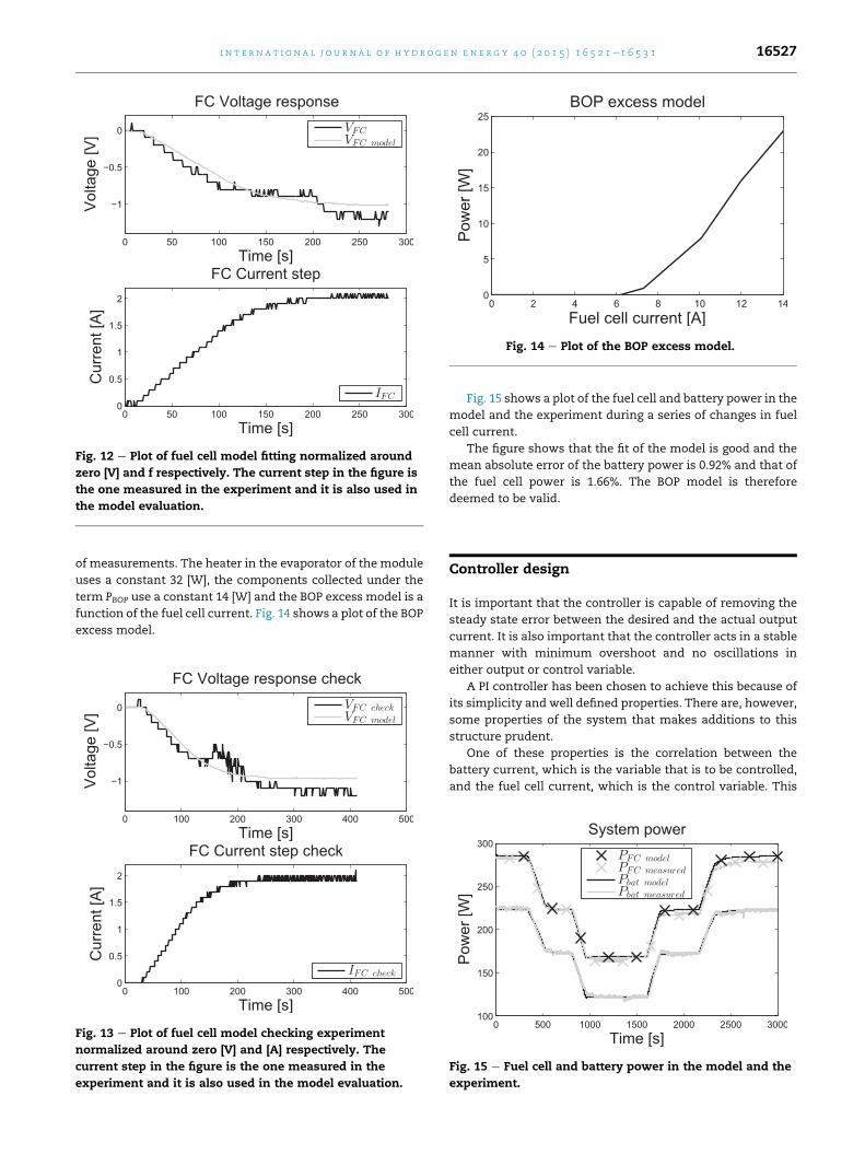
Fig. 12 e Plot of fuel cell model fitting normalized around

zero [V] and f respectively. The current step in the figure is

the one measured in the experiment and it is also used in

the model evaluation.

Fig. 14 e Plot of the BOP excess model.

i n t e r n a t i o n a l j o u r n a l o f h y d r o g e n en e r g y 4 0 ( 2 0 1 5 ) 1 6 5 2 1e1 6 5 3 1 16527

of measurements. The heater in the evaporator of the module

uses a constant 32 [W], the components collected under the

term PBOP use a constant 14 [W] and the BOP excess model is a

function of the fuel cell current. Fig. 14 shows a plot of the BOP

excess model.

Fig. 13 e Plot of fuel cell model checking experiment

normalized around zero [V] and [A] respectively. The

current step in the figure is the one measured in the

experiment and it is also used in the model evaluation.

Fig. 15 shows a plot of the fuel cell and battery power in the

model and the experiment during a series of changes in fuel

cell current.

The figure shows that the fit of the model is good and the

mean absolute error of the battery power is 0.92% and that of

the fuel cell power is 1.66%. The BOP model is therefore

deemed to be valid.

Controller design

It is important that the controller is capable of removing the

steady state error between the desired and the actual output

current. It is also important that the controller acts in a stable

manner with minimum overshoot and no oscillations in

either output or control variable.

A PI controller has been chosen to achieve this because of

its simplicity and well defined properties. There are, however,

some properties of the system that makes additions to this

structure prudent.

One of these properties is the correlation between the

battery current, which is the variable that is to be controlled,

and the fuel cell current, which is the control variable. This

Fig. 15 e Fuel cell and battery power in the model and the

experiment.

Fig. 17 e Negative step in battery current set point

performed in the model. IFC model RAW is the fuel cell voltage

set point before the rate limiter.

i n t e rn a t i o n a l j o u r n a l o f h y d r o g e n en e r g y 4 0 ( 2 0 1 5 ) 1 6 5 2 1e1 6 5 3 116528

means that using a feedforward of the output current set point

is ideal.

The second addition to the PI controller structure is due to

the limited rate of change imposed on the control variable IFCby the system dynamics described in Section 1. This means

that there is a risk of integrator windup, leading to controller

instability [[18], p.80]. It is therefore chosen to include an anti-

windup in the controller. The alternative to the anti windup is

to tune the controller so conservatively that the largest

possible changes in reference are performed without integral

windup. This would make the response of the controller very

slow and is therefore undesirable.

Fig. 16 shows a block diagram of the controller.

Investigation of measurements shows that the average

difference between the fuel cell current and the output cur-

rent is 3 [A]. The feedforward constant is therefore set to

Kff ¼ 3.

The other controller constants are tuned iteratively using

the model, and Kp ¼ 0.0240 and Ki ¼ 0.0192 are found to give a

good compromise between stability and fast settling. There

are many possible policies for setting KAW, but it is generally

recommended that is set to a larger or equal value to Ki [[18],

p.85]. The reason is that the anti-windup should be able to

react as quickly as the buildup of the integral compensation.

Here KAW is set to the same value as Ki based on model

simulations.

Fig. 17 shows a representative negative step response from

the model using these constants and Fig. 18 shows a repre-

sentative positive step response.

Here, and in the rest of this work, the load current is zero

and the modules output current is equal to the battery

current.

In both of the step responses, the fuel current follows the

rate limiter until just before the module's output current rea-

ches its set point.While the fuel cell current is rate limited, the

anti-windup limits the raw controller output IFC model RAW.

When the output current comes close to the set point, the

anti-windup stops being active, and the controller leads the

output current smoothly to its final value.

To illustrate the usefulness of the anti-windup, a step

similar to the one in Fig. 18 is performed without anti-windup

and plotted in Fig. 19.

Fig. 16 e Diagram of the output current controller.

Here it is apparent that integrator windup occurs and a

large overshoot in the output current is the result.

As Figs. 18 and 17 illustrate, the controller with its anti-

windup and feedforward works well in the model without

overshoot or oscillations in the output or control variables. It

is therefore concluded that the developed controller should be

tested in the H3 350 module.

Fig. 18 e Positive step in output current set point

performed in the model. IFC model RAW is the fuel cell voltage

set point before the rate limiter.

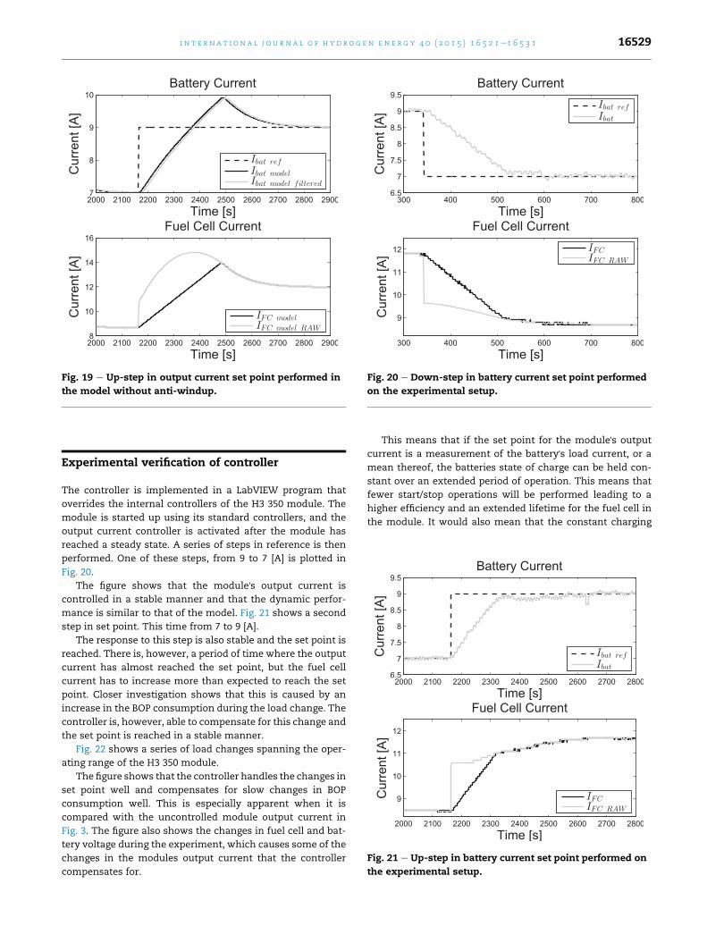
Fig. 19 e Up-step in output current set point performed in

the model without anti-windup.

Fig. 20 e Down-step in battery current set point performed

on the experimental setup.

Fig. 21 e Up-step in battery current set point performed on

the experimental setup.

i n t e r n a t i o n a l j o u r n a l o f h y d r o g e n en e r g y 4 0 ( 2 0 1 5 ) 1 6 5 2 1e1 6 5 3 1 16529

Experimental verification of controller

The controller is implemented in a LabVIEW program that

overrides the internal controllers of the H3 350 module. The

module is started up using its standard controllers, and the

output current controller is activated after the module has

reached a steady state. A series of steps in reference is then

performed. One of these steps, from 9 to 7 [A] is plotted in

Fig. 20.

The figure shows that the module's output current is

controlled in a stable manner and that the dynamic perfor-

mance is similar to that of the model. Fig. 21 shows a second

step in set point. This time from 7 to 9 [A].

The response to this step is also stable and the set point is

reached. There is, however, a period of time where the output

current has almost reached the set point, but the fuel cell

current has to increase more than expected to reach the set

point. Closer investigation shows that this is caused by an

increase in the BOP consumption during the load change. The

controller is, however, able to compensate for this change and

the set point is reached in a stable manner.

Fig. 22 shows a series of load changes spanning the oper-

ating range of the H3 350 module.

The figure shows that the controller handles the changes in

set point well and compensates for slow changes in BOP

consumption well. This is especially apparent when it is

compared with the uncontrolled module output current in

Fig. 3. The figure also shows the changes in fuel cell and bat-

tery voltage during the experiment, which causes some of the

changes in the modules output current that the controller

compensates for.

This means that if the set point for the module's output

current is a measurement of the battery's load current, or a

mean thereof, the batteries state of charge can be held con-

stant over an extended period of operation. This means that

fewer start/stop operations will be performed leading to a

higher efficiency and an extended lifetime for the fuel cell in

the module. It would also mean that the constant charging

Fig. 22 e Series of step responses performed on the experimental setup.

i n t e rn a t i o n a l j o u r n a l o f h y d r o g e n en e r g y 4 0 ( 2 0 1 5 ) 1 6 5 2 1e1 6 5 3 116530

and discharging of the battery can be minimized, leading to a

reduced energy loss in the battery because less current is

passed through its internal resistance.

Conclusions

In this work a model of the relationship between fuel cell and

output current of a H3 350 reformedmethanol fuel cellmodule

produced by Serenergy has been produced and used to

develop an output controller.

Themodel has threemain parts: a batterymodel, a fuel cell

model and a BOP model.

The battery model consists of an open circuit voltage and

an equivalent circuit model and was found to have a mean

absolute error of 1.2% on its fitting data and 4.15% on its

checking data.

The fuel cell model consists of a polarization curve with

added first order dynamics. This model has a mean absolute

error of 11.8% on its fitting data and 14.9% on its checking data.

The BOP model includes constant contributions from a

heater in the evaporator, constant contributions from other

BOP components such as controllers and pumps and a term

that is dependent on the fuel cell current. This model is found

to have a mean absolute error of 0.92% when comparing the

battery current in the model and the experiment.

This model was used to develop a controller for the output

current of the module which uses a PI controller with feed-

forward and anti-windup. This controller is tested in the

model and in the H3 350 module. The controller is found to

function as intended and it is concluded that the controller

could have applications in state of charge control in systems

with batteries and reformed methanol fuel cells. This state of

charge control could lead to an extended lifetime for the fuel

cell because of fewer start/stop operations and a higher sys-

tem efficiency due to less charging and discharging of the

battery in the system.

Future work

There are areas where the models developed in this work

could be improved. Disturbance models could for example be

included. These disturbances include changes in battery load

current or the slow change in BOP consumption, mentioned in

the previous section.

The controller developed in this work functions well, but if

more models of measured disturbances where developed, a

model predictive control could be employed instead to

compensate for these, as it is done for a conventional fuel cell

system in Ref. [19].

i n t e r n a t i o n a l j o u r n a l o f h y d r o g e n en e r g y 4 0 ( 2 0 1 5 ) 1 6 5 2 1e1 6 5 3 1 16531

Acknowledgment

We gratefully acknowledge the financial support of the EUDP

program and the cooperation of Serenergy A/S.

r e f e r e n c e s

[1] Dutta S. A review on production, storage of hydrogen and itsutilization as an energy resource. J Ind Eng Chem2014;20(4):1148e56. http://dx.doi.org/10.1016/j.jiec.2013.07.037.

[2] Satyapal S, Petrovic J, Read C, Thomas G, Ordaz G. The U.S.department of energy's national hydrogen storage project:progress towards meeting hydrogen-powered vehiclerequirements. Catal Today 2007;120:246e56. http://dx.doi.org/10.1016/j.cattod.2006.09.022.

[3] Serenergy a/s home page, http://www.serenergy.com/(July2015).

[4] Zhang J, Xie Z, Zhang J, Tang Y, Songa C, Navessin T, et al.High temperature PEM fuel cells. J Power Sources2006;160:872e91. http://dx.doi.org/10.1016/j.jpowsour.2006.05.034.

[5] Andreasen SJ, Vang JR, Kær SK. High temperature PEM fuelcell performance characterisation with co and co2 usingelectrochemical impedance spectroscopy. Int J HydrogenEnergy 2011;36:9815e30. http://dx.doi.org/10.1016/j.ijhydene.2011.04.06.

[6] Justesen KK, Andreasen SJ, Shaker HR. Dynamic modeling ofa reformed methanol fuel cell system using empirical dataand adaptive neuro-fuzzy inference system models. J FuelCell Sci Technol 2013;11. http://dx.doi.org/10.1115/1.4025934.021004 e 021004e8.

[7] Chrenko D, Gao F, Blunier B, Bouquain D, Miraoui A.Methanol fuel processor and PEM fuel cell modeling formobile application. Int J Hydrogen Energy 2010;35:6863e71.http://dx.doi.org/10.1016/j.ijhydene.2010.04.022.

[8] Kolb G, Keller S, Tiemann D, Schelhaas K-P, Schurer J,Wiborg O. Design and operation of a compact microchannel5 kw el,net methanol steam reformer with novel pt/in2o3catalyst for fuel cell applications. Chem Eng J2012;207:388e402. http://dx.doi.org/10.1016/j.cej.2012.06.141.22nd International Symposium on Chemical ReactionEngineering (ISCRE 22).

[9] Hulteberg P, Porter B, Silversand F, Woods R. A versatile,steam reforming based small-scale hydrogen productionprocess. In: 16th world hydrogen energy conference; 2006.WHEC 2006.

[10] Yousfi-Steiner N, Mocoteguy P, Candusso D, Hissel D. Areview on polymer electrolyte membrane fuel cell catalystdegradation and starvation issues: causes, consequencesand diagnostic for mitigation. J Power Sources2009;194:130e45. http://dx.doi.org/10.1016/j.jpowsour.2009.03.060.

[11] Mitsuda K, Murahashi T. Air and fuel starvation ofphosphoric acid fuel cells: a study using a single cell withmulti-reference electrodes. J Appl Electrochem1991;21:524e30. http://dx.doi.org/10.1007/BF01018605.

[12] Schmidt TJ, Baurmeister J. Properties of high-temperaturePEFC Celtec-P 1000 MEAS in start/stop operation mode. JPower Sources 2008;176(2):428e34. http://dx.doi.org/10.1016/j.jpowsour.2007.08.055. selected Papers presented at the10th{ULM} ElectroChemical Days W. Tillmetz, J. Lindenmayer10th Ulm ElectroChemical Days.

[13] Seaman A, Dao T-S, McPhee J. A survey of mathematics-based equivalent-circuit and electrochemical battery modelsfor hybrid and electric vehicle simulation. J Power Sources2014;256:410e23. http://dx.doi.org/10.1016/j.jpowsour.2014.01.057.

[14] Korsgaard AR, Nielsen MAP, Bang M, Kær SK. Modeling of coinfluence in pbi electrolyte PEM fuel cells. In: ASME 2006 4thinternational conference on fuel cell science, engineeringand technology; 2006. http://dx.doi.org/10.1115/FUELCELL2006e97214.

[15] Ohs JH, Sauter U, Maass S, Stolten D. Modeling hydrogenstarvation conditions in proton-exchange membrane fuelcells. J Power Sources 2011;196(1):255e63. http://dx.doi.org/10.1016/j.jpowsour.2010.06.038.

[16] Niya SMR, Hoorfar M. Study of proton exchange membranefuel cells using electrochemical impedance spectroscopytechnique: a review. J Power Sources 2013;240:281e93. http://dx.doi.org/10.1016/j.jpowsour.2013.04.011.

[17] Keesman KJ. System identification, an introduction.Springer; 2011.

[18] Astrom K, Hagglund T. PID controllers: theory, design, andtuning. 2nd ed. Instrument Society of America; 1995.

[19] Bordons C, Ridao MA, Perez A, Arce A, Marcos D. Modelpredictive control for power management in hybrid fuel cellvehicles. In: Vehicle power and propulsion conference IEEE;2010. http://dx.doi.org/10.1109/VPPC.2010.5729119.