modeling and inversion of magnetic and ip/resistivity …
TRANSCRIPT

MODELING AND INVERSION OF MAGNETIC AND IP/RESISTIVITY DATA FOR DELINEATING
FAVOURABLE TARGET AREAS FOR URANIUM MINERALIZATION IN CHHOTA UDAIPUR, AJMER
DISTRICT, RAJASTHAN
by CHINNAMILLI RAMANJANEYULU
ENGG1G201801005
Bhabha Atomic Research Centre, Mumbai
A thesis submitted to the
Board of Studies in Engineering Sciences
In partial fulfillment of requirements
for the Degree of
MASTER OF TECHNOLOGY
of
HOMI BHABHA NATIONAL INSTITUTE
February, 2021


ACKNOWLEDGEMENT
My greatest appreciation goes to my project Guide, Dr. V. Ramesh Babu, Adjunct
Professor, HBNI for his valuable support and decisive guidance throughout this thesis work.
His support in suggesting valuable reference books, in sharing his field and research
experience contributed greatly to enrich my thesis.
I have great pleasure in acknowledging my gratitude to my technical advisor Shri
Prakash Mukherjee, SO/D, Exploration Geophysics group, AMD, Jaipur for his honest and
constructive comments in data processing and interpretation.
I am grateful to Dr. D. K. Sinha, Director, Atomic Minerals Directorate for
Exploration & Research (AMD), Department of Atomic Energy (DAE) who has given me
the opportunity to do M. Tech Degree course from HBNI through BARC training school.
I also wish my thanks with deeper sense of gratitude to Additional Director (OP-I),
Additional Director (OP-II), Additional Director R & D for their guidance and support.
I would also like to thank Regional Director, AMD, WR and Deputy Regional
Director AMD, WR for his continuous support and discussions at various steps during this
thesis work and help for submitting thesis within given time frame.
My special thanks go to Shri A. Markandeyulu, Incharge, EGP Group, AMD-
Hyderabad and Shri Subash Ram, Incharge, EGP Group, AMD-Jaipur.
I would like to thank Shri Roshan Ali Shaik (SO/D), Y. Siva Krishna (SO/D), Shri
Deepak Kumar (SO/D), Shri Rajesh Kumar Verma (SO/D), D. Damodhar (SO/C), Shri D.
Raghavender (SO/C), of EGPG, AMD, WR and Shri B. Srinivas Rao (SO/E), Shri T. Manoj
Kumar (SO/C) of AMD, SR, Shri Harsha Yalla, SO/D (ASRS) for their support and helpful
discussions.

I would also like to thank incharge Petrology laboratory and XRF laboratory, AMD,
WR for their support and My acknowledgement would be incomplete without thanking
Incharge and Head BARC Training School, AMD Campus, Hyderabad for their support
and for ensuring the optimum academic environment that has helped me in completion of
the project.
I am also thankful to the competent authority of HBNI for providing the opportunity to
pursue the M. Tech. degree.
I also thankful to my colleagues, all technical and non-technical staff who have
supported me directly or indirectly in the completion of my project work
i
CONTENTS
……………………………....
SYNOPSIS iv
LIST OF FIGURES v
LIST OF TABLES ix
CHAPTER 1 INTRODUCTION
1.1 General 1
1.2 Geophysical methods for uranium exploration 2
1.2.1 Magnetic method 3
1.2.2 Induced polarization (IP) and Electrical resistivity methods 4
1.3 Study area 4
1.3.1 Objective of the study 4
1.3.2 Location and accessibility of the study area 5
1.3.3 Previous work 6
CHAPTER 2 GEOLOGY OF THE STUDY AREA
2.1 Introduction 11
2.2 Regional geology of the area 12
2.2.1 Banded Gneissic Complex 13
2.3 Detailed geology of the study area 14
CHAPTER 3 MAGNETIC METHOD OF EXPLORATION
3.0 Introduction 17
3.1 Theory of magnetic method 18
3.2 Instruments 19
3.3 Magnetic Data Acquisition 20
3.4 Physical property measurement 21

ii
3.5 Magnetic Data processing 22
3.5.1 Diurnal correction 23
3.5.2 Correction for cultural noise 24
3.5.3 Data visualization 24
3.5.4 Filtering techniques 24
3.6 Interpretation of Magnetic Data 25
3.6.1 Qualitative interpretation 26
3.6.1.1Total Magnetic Intensity Anomaly Map 26
3.6.1.2 Reduced to Pole Magnetic Anomaly Map 27
3.6.1.3 Upward continuation filter 29
3.6.1.4 First Vertical Derivative Filter 30
3.6.1.5 Tilt Derivative or Tilt angle method 32
3.6.2 Quantitative interpretation of magnetic data 33
3.6.2.1 Euler deconvolution 34
3.6.3 Modeling and Inversion of Magnetic Data 36
3.6.3.1 2-D Forward Modeling 36
3.6.3.2 3-D Modeling 39
3.6.3.3 Forward modeling in 3D 43
CHAPTER 4 INDUCED POLARIZATION AND RESISTIVITYMETHOD OF
EXPLORATION
4.1 Introduction 47
4.2 Theory of Induced polarization 48
4.2.1 Membrane polarization 49
4.2.2 Electrode polarization 49
4.3 Measurement of Induced Polarization 50
4.4 Theory of DC Resistivity method 51

iii
4.5 Data Acquisition of IP and Resistivity Data 54
4.5.1 Instrumentation 54
4.5.2 Gradient array 54
4.5.3 Data acquisition 55
4.6 Processing and interpretation of IP and Resistivity Data 57
4.6.1 Apparent Resistivity Map 57
4.6.2 Apparent Chargeability Map 58
4.6.3 Decay curve analysis of IP data 60
4.7 Inversion of IP/Resistivity Data 64
CHAPTER 5 INTEGRATED INTERPRETATION
5.1 Petrographic Study 69
5.2 Hydrogeochemical study 70
5.3 Geochemical analysis 72
5.4 Profile analysis of Magnetic and IP/Resistivity data 75
CHAPTER 6 CONCLUSIONS 81
PUBLICATION TITLE 83
REFERENCES 85

iv
SYNOPSIS
This thesis for the M. Tech project through HBNI deals with the systematic
application of Magnetic and IP/Resistivity methods to identify the subsurface target areas
for uranium mineralisation in and around Chhota Udaipur, Ajmer district, Rajasthan. The
study area is located around 9 km south-east of Kishangarh which is a part of the banded
gneissic complex (BGC) of Archaean age. Radioactive anomalies with high uranium
concentration were reported during geological investigation in 1997-98 by AMD. The study
area gained more importance as it is located within the albitite zone in its southern part
which is important in the NDFB for its correlation with U mineralization in several areas
like Rohil-Ghateswar sector of Sikar district, Rajasthan. Magnetic and IP/Resistivity
methods are applied to delineate the structural features like faults/fractures, shear zones and
conductive bodies which form the ideal environment for U-mineralization.
Magnetic data was acquired over the 30 sq.km area which facilitated in demarcating
faults/fractures in E-W, NE-SW and NW-SE directions. Three significant high magnetic
anomalies have been observed in the middle and towards southeastern side of study area,
interpreted as mafic intrusion/ magnetite mineralization in BGC. 2-D and 3-D magnetic
models enabled in deciphering the location and geometry of the structures in the study area.
From IP/Resistivity data over 7.5 sq.km area, three high chargeability zones have been
delineated, zone-M1 has NE-SW strike length of around 600 m with width of 90 to 130 m
and zone-M2 has strike length of 1.5 km with width of 300 to 350 m in NNE-SSW direction
in the eastern side of the study area. The high chargeability zones are correlatable with low
to moderate resistivities which are interpreted as the fractures filled with disseminated
sulphides in BGC. Laboratory analysis of rock samples and water samples were carried out
for better correlation with the observed geophysical anomalies with laboratory values.
Integrated interpretation of geophysical data including petrographic study,
geochemical and hydro geochemical studies reveal that high chargeability zones are well
correlated with the moderate to low resistivity and moderate to high magnetic zones. These
zones are favorable target areas for sub-surface uranium mineralization in this area.
v
LIST OF FIGURES
Figure No. Description
Page NO.
1.1 Location of the study area, Chhota udaipur village, Ajmer district,
Rajasthan
5
1.2 Survey block over toposheet No. 45J/14 & 15, Chhota udaipur area,
Ajmer district , Rajasthan
6
1.3 Previous geophysical Total magnetic anomaly map, Chhota
Udaipur area, Ajmer district, Rajasthan
8
1.4 Previous geophysical apparent chargeability contour map, Chhota
Udaipur area, Ajmer district, Rajasthan
9
2.1 Three sub-basins of North Delhi Fold Belt, two sub-parallel
albitite zone present in the Khetri Sub-Basin and BGC
13
2.2 Geological map of Tilonia-Nasirabad area, Ajmer district,
Rajasthan
16
3.1 GEM Systems, GSM 19T Proton Precision Magnetometer used
for Data Acquisition in the survey area
19
3.2 Magnetic profile layout map, Chhota Udaipur area, Ajmer district,
Rajasthan
20
3.3 Diurnal variation of geomagnetic field on 17th December 2019 23
3.4 Total magnetic intensity anomaly map, Chhota Udaipur area,
Ajmer district , Rajasthan
27
3.5 Reduced to pole anomaly map, Chhota Udaipur area, Ajmer
district , Rajasthan
28
3.6 Upward continued magnetic (RTP) map of 400m level, Chhota
Udaipur area, Ajmer district, Rajasthan
30
vi
3.7 FVD of TMI anomaly map, Chhota Udaipur area, Ajmer district,
Rajasthan
31
3.8 Tilt-Angle map of the RTP grid, Chhota Udaipur area, Ajmer
district , Rajasthan
33
3.9 Euler solutions over TMI map, Chhota Udaipur area, Ajmer
district , Rajasthan
35
3.10 Profile AB over TMI map for 2D modeling 37
3.11 2D geological model of profile AB, Chhota Udaipur area, Ajmer
district , Rajasthan
38
3.12 3-D Inverted Magnetic model of Chhota Udaipur area, Ajmer
district , Rajasthan
41
3.13 Inverted magnetic model highlighting the high susceptibility bodies
overlaid on the rtp map, chhota udaipur area, Ajmer district,
Rajasthan
42
3.14 Horizontal depth slices of inverted magnetic model at a depth of
200m, 400m and 600m
43
3.15 TMI map and 3D modelled TMI map response 44
3.16 3D forward modeling for observed TMI response 45
4.1 (A) Membrane polarization (B) Electrode polarization 50
4.2 IP measurement 51
4.3 Schematic diagram for the resistivity(𝜌) when current passes
through a material
52
4.4 General electrode configuration used in resistivity survey 53
4.5 Multi electrode IRIS IP Receiver 54
vii
4.6 IRIS IP Transmitter 54
4.7 Gradient array configuration 55
4.8 IP/Resistivity Profiles layout over RTP map, Chhota Udaipur area,
Ajmer district , Rajasthan
56
4.9 Apparent resistivity map, Chhota-Udaipur area, Ajmer district,
Rajasthan
58
4.10 Apparent chargeability map, Chhota-Udaipur area, Ajmer district,
Rajasthan
60
4.11 Chargeability decay curve analysis of IP data station near RW1 62
4.12 Chargeability decay plot analysis of IPdata station near RW2 62
4.13 Bivariate plot of Chargeability (a) & Decay Time constant(τ1) 63
4.14 Bivariate plot of Chargeability(b) & Decay Time constant(τ2) 63
4.15 2D-Inverted depth sections (P) resistivity (Q) Chargeability of
IP/Resistivity data along the traverse S8E
66
4.16 2-D Inverted depth-sections of Chargeability along the traverses
S6, S7 and S8, Chhota Udaipur area, Ajmer district, Rajasthan
67
4.17 2-D Inverted depth-sections of Resistivity along the traverses S6,
S7 and S8, Chhota Udaipur area, Ajmer district, Rajasthan
68
5.1 Petrographic study of radioactive sample 69
5.2 Petrographic study of grab sample 70
5.3 Petrographic study of grab sample 70
5.4 Water sample locations over the RTP map of Chhota Udaipur area,
Ajmer district , Rajasthan
71
viii
5.5 Correlation of major oxides 74
5.6 Primitive Mantle normalized spider plot 74
5.7 Profiles over RTP and Apparent chargeability maps 75
5.8 Profile analysis of magnetic and IP/Resistivity data
along RW1 line
76
5.9 Profile analysis of magnetic and IP/Resistivity data
along RW2 line
77
5.10 (a) Integrated structural features and high chargeability zones over
FVD of RTP map (b) Resistivity contour map of Chhota Udaipur
area, Ajmer district, Rajasthan
78

ix
LIST OF TABLES
Table No. Description Page No.
2.1 Stratigraphic Classification of Bhilwara Supergroup 15
3.1 Physical properties of various rock samples from Chhota Udaipur,
Ajmer district, Rajasthan 22
3.2 Different rock types and their magnetic susceptibility for the model
of AB profile 39
3.3 Inversion parameters of 3D magnetic voxel model 40
4.1 Inversion parameters of chargeability and resistivity depth section
of S8E line 64
4.2 Inversion parameters of chargeability and resistivity depth sections
of S6, S7 and S8 lines 65
5.1 Hydrogeochemical analysis of water samples from Chhota
Udaipur area, Ajmer district, Rajasthan 73


1
CHAPTER 1
INTRODUCTION
1.1 General
Fossil fuel sources are gradually declining, leading to a potential global scarcity of energy.
Nuclear power is a long-term, low-carbon and cleaner solution to meet the requirements of
increasing population in our country and it has a very significant economic and operational
advantages over other conventional sources of power. It produces energy via nuclear fission
rather than chemical burning and it contributes 34% reduction in carbon intensity per MW than
renewable (world nuclear news 2020), the noxious element of global warming. A pellet of
nuclear fuel weighs approximately 6 grams. However, that single pellet yields the amount
of energy equivalent to that generated by a ton of coal, 120 gallons of oil or 17,000 cubic
feet of natural gas, making nuclear fuel much more efficient than fossil fuels
(https://www.world-nuclear.org). Uranium is the raw material mostly used to create fuel for
nuclear power and its atomic number 92 and atomic weight 238 which is highest atomic
number found naturally in significant quantity. The average abundance of uranium in crustal
rocks is 2.7 ppm (2-4 ppm various estimates) (IAEA Vienna, 1988). As demand for the energy
is steeply increasing, uranium consumption is also increasing and hence, it has become
mandatory to find new uranium reserve in our country.
Geophysical techniques have been successfully employed worldwide for delineation
of mineral resources. Geophysical methods are indirect tools for uranium exploration which
play a vital role in the identification of subsurface structural features and possible
conducting horizons as favorable locales for uranium mineralization.
The most obvious technique to explore for uranium deposits is the radiometric
method that directly records the response of uranium and other radioactive elements by

2
measuring gamma rays. Anomalous concentration may be detected by radiometric surveys
using scintillometers and Geiger-muller counters over the subsurface structures containing
radioactive materials in the top 30 cm of the earth’s cover as gamma rays emanating from
the earth’s surface below 30 cm will not be detected by surface measurements of
radioactivity. Therefore, geophysical methods are applied as an indirect tool to explore the
concealed of uranium mineralization at depths, even up to 1 km.
Geophysical methods are successfully employed in discovery of the world-famous
uranium deposits like Olympic dam deposit (Esdale Donald et al., 2003) and McArthur River
mine (Tuncer et al., 2006), Millennium zone (Powell et al., 2007) of Athabasca basin.
1.2 Geophysical methods for uranium exploration
Uranium minerals does not occur in appreciable quantity to alter the physical properties
of rock to provide detectable geophysical anomaly. However, like any other minerals uranium
gets deposited where it finds the suitable environment for precipitation. Geophysical methods
utilized to detect subsurface geological targets often associated with uranium mineralization,
for example fracture, faults, lithological contacts. The geometry of the subsurface structural
features with appreciable physical property contrast can be mapped well by application of
geophysical methods. The geophysical methods which are widely used are gravity, magnetic
methods in the regional and semi-regional scales; and, electromagnetic and geoelectrical
methods which include Induced Polarization technique for detailed investigations on prospect
scale. In general, the choice of any geophysical method for uranium exploration largely
depends upon the local geology of the area under investigation. The utility of any geophysical
methods depends on the physical property contrast between the geological object sought and
its host rocks. Although, a wide range of geophysical methods are available for uranium
exploration, the most useful methods are the magnetic, electrical, gravity and electromagnetic.

3
However, based on the geological problem magnetic and IP/Resistivity methods are opted for
the present study and their applicability discussed briefly below.
1.2.1 Magnetic method
Magnetic method is a versatile, easy and inexpensive geophysical tool that can be
executed fast. It is a useful technique both for reconnaissance and detailed investigations such
as geological mapping and delineation of structural features. Intrusive bodies can be effectively
delineated by the magnetic method. The magnetic method of prospecting is based on the study of
local geomagnetic field produced by the variations in intensity of magnetization of rock formations.
The magnetization of rocks is partly due to induction in the earth's magnetic field and to some
extent due to remnant magnetization of the underlying formations. The induction component
depends on magnetic susceptibility (k) of rocks and on the intensity of magnetic field. The variable
concentration of ferrimagnetic minerals plays a key role in determining the magnetic properties
of the rock that are significant geologically and geophysically. While the magnetizing field
remains constant over a small area, the remnant magnetic intensity and its variation for a given
rock type also remain the same. In turn, the variation in the measured magnetic field can be
attributed to the presence of various rock types with different susceptibilities. Therefore, magnetic
method can be used effectively for geological mapping and structural studies. Therefore, zones
favourable for uranium accumulation can be identified by surface magnetic observations. The
successful application magnetic method to delineate the subsurface structural features like
faults, fractures, shear zones and alteration zones for uranium exploration in India discussed
by Dash et al., 2006, Ramesh babu et al., 2007, Satyanarayana et al., 2014, and Shrajala et al.,
2015.World class ore bodies like the Olympic dam(Esdale Donald et al., 2003), Ernest
Henry(Austin et al., 2019) of Australia and Bayon Obo (Hong et al., 2016) associated with iron
oxide related mineralisation were established based on magnetic method.
4
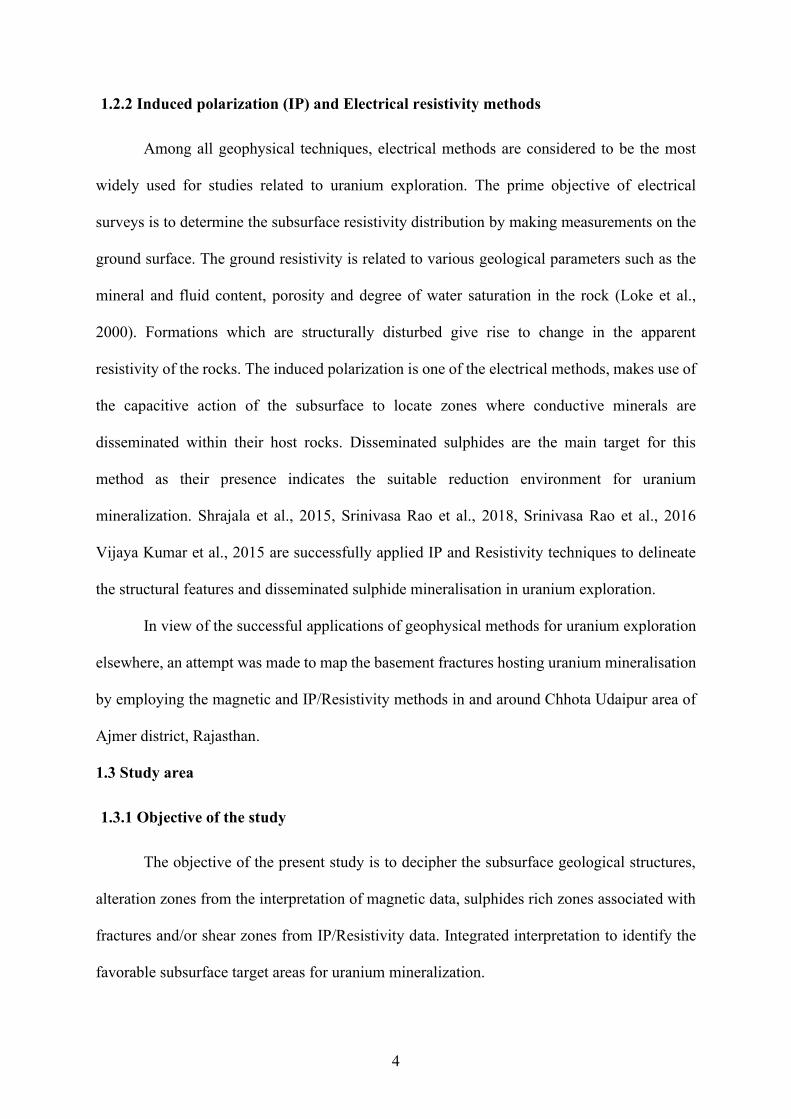
1.2.2 Induced polarization (IP) and Electrical resistivity methods
Among all geophysical techniques, electrical methods are considered to be the most
widely used for studies related to uranium exploration. The prime objective of electrical
surveys is to determine the subsurface resistivity distribution by making measurements on the
ground surface. The ground resistivity is related to various geological parameters such as the
mineral and fluid content, porosity and degree of water saturation in the rock (Loke et al.,
2000). Formations which are structurally disturbed give rise to change in the apparent
resistivity of the rocks. The induced polarization is one of the electrical methods, makes use of
the capacitive action of the subsurface to locate zones where conductive minerals are
disseminated within their host rocks. Disseminated sulphides are the main target for this
method as their presence indicates the suitable reduction environment for uranium
mineralization. Shrajala et al., 2015, Srinivasa Rao et al., 2018, Srinivasa Rao et al., 2016
Vijaya Kumar et al., 2015 are successfully applied IP and Resistivity techniques to delineate
the structural features and disseminated sulphide mineralisation in uranium exploration.
In view of the successful applications of geophysical methods for uranium exploration
elsewhere, an attempt was made to map the basement fractures hosting uranium mineralisation
by employing the magnetic and IP/Resistivity methods in and around Chhota Udaipur area of
Ajmer district, Rajasthan.
1.3 Study area
1.3.1 Objective of the study
The objective of the present study is to decipher the subsurface geological structures,
alteration zones from the interpretation of magnetic data, sulphides rich zones associated with
fractures and/or shear zones from IP/Resistivity data. Integrated interpretation to identify the
favorable subsurface target areas for uranium mineralization.
5
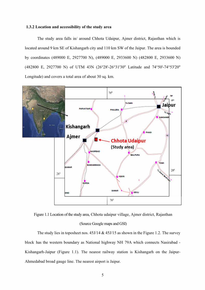
1.3.2 Location and accessibility of the study area
The study area falls in/ around Chhota Udaipur, Ajmer district, Rajasthan which is
located around 9 km SE of Kishangarh city and 110 km SW of the Jaipur. The area is bounded
by coordinates (489000 E, 2927700 N), (489000 E, 2933600 N) (482800 E, 2933600 N)
(482800 E, 2927700 N) of UTM 43N (26°28'-26°31'30'' Latitude and 74°50'-74°53'20''
Longitude) and covers a total area of about 30 sq. km.
Figure 1.1 Location of the study area, Chhota udaipur village, Ajmer district, Rajasthan
(Source Google maps and GSI)
The study lies in toposheet nos. 45J/14 & 45J/15 as shown in the Figure 1.2. The survey
block has the western boundary as National highway NH 79A which connects Nasirabad -
Kishangarh-Jaipur (Figure 1.1). The nearest railway station is Kishangarh on the Jaipur-
Ahmedabad broad gauge line. The nearest airport is Jaipur.

6
Figure 1.2 Survey block over toposheet No. 45J/14 & 15, Chhota udaipur area, Ajmer district,
Rajasthan (Source SOI)
1.3.3 Previous work
Uraniferous polymetallic veins are reported in the gneisses of Sandmata Complex of
Archaean age by Sinha et al., 2002, from two adjoining dug well dump samples near Chhota
Udaipur village. These samples are analyzed by laboratory studies of gamma-ray spectrometry,
fused pellet fluorimetry for uranium along with physical and chemical methods. Laboratory
studies revealed that the presence 1.62 % of eU3O8, approximately 10% of ThO and Cu, Mo,
and Pb vary from 0.41 to 10.64%, 0.03 to 0.46% and <0.02 to 0.11% respectively and also
some samples were analyzed more than 1% of sulphides (Sinha et al., 2002). These results
7
shown that samples have a polymetallic character and as the two dug wells are separated by
210 m distance in NE-SW direction, indicates a possible subsurface strike continuity.
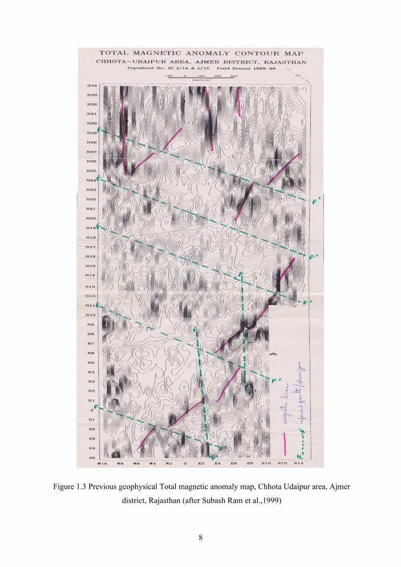
Geophysical studies comprising magnetic, IP/Resistivity and EM-Turam surveys were
carried out earlier by Subash Ram et al., (1999) to trace the subsurface sulphide bearing zones
towards NE direction of radioactive anomaly location over an area of 4 Sq. Km near Chhota
Udaipur area, Ajmer district, Rajasthan. The study indicated the presence of high magnetic
linear with 300-1500 nT amplitude and which is truncated at many places, by N-S trending
local displacements. High chargeability zones with amplitude 16 mV/V were observed with a
background of 5 mV/V as isolated pockets by the Induced polarization/ Resistivity survey. The
geophysical signatures are interpreted to be due to the fault/fractures filled with sulphides in a
high resistive environment like banded gneissic complex (BGC) of Archaean age. In view of
the encouraging results obtained from the earlier geophysical surveys, magnetic and
IP/Resistivity techniques are adopted to delineate the favourable zones of uranium
mineralization in the area.
8
Figure 1.3 Previous geophysical Total magnetic anomaly map, Chhota Udaipur area, Ajmer
district, Rajasthan (after Subash Ram et al.,1999)

9
Figure 1.4 Previous geophysical apparent chargeability contour map, Chhota Udaipur area,
Ajmer district, Rajasthan (after Subash Ram et al.,1999).


11
CHAPTER 2
GEOLOGY OF THE STUDY AREA
2.1 Introduction
North-western Indian Craton (NWIC) presents varied geological and tectonic process
of over 3500 million years. The NWIC is bounded by Great Boundary Fault (GBF) in the east
and Thar Desert in the west. It is separated by the SONATA (Son-Naramada-Tapti) lineament
from the Central Indian Tectonic Zone in the south and Indo-Gangetic alluvium in the north
(Ramakrishnan et al., 2010; Dhirenda Kumar Pandey et al., 2014). It hosts variety of metallic
and non-metallic and mineraloid deposits of sizeable mineral reserves (Sumit Kumar Ray et
al., 1987). The terrain consists of wide variety of litho-units from Archaean to Holocene. The
oldest geological record is contained within Banded Gneissic Complex (BGC) formed during
the Archaean period. Aravalli Basin and Delhi Basin formed during Proterozoic period due to
repeated period of crustal rifting, development of intracontinental rift basins, subsequent
oceanic trough and depositions of sediments of different facies. The formation of folded belts
associated with multi deformation and polyphase metamorphism of the rock sequences. During
the late Proterozoic period, crustal deformation and associated thermal regime caused large
scale anatexis and emplacement of number of granite plutons and wide spread acidic and local
basic volcanism and associated mineralisation. During Phanerozoic period the extent of
geological activity has reduced substantially except the development of separate basins. The
period is followed by the episodes of extensive basaltic volcanism, Deccan traps during Late
Cretaceous to Early Tertiary period which is present on the southern part of the craton. Finally,
depositions of fluvial sediments, formation of aeolian land forms are prevailed during the
Holocene period (Sinha and Roy, 1998).
12
2.2 Regional geology of the area
The Banded Gneissic complex of Archean age forms the basement and comprises of high
grade metamorphic and migmatite rocks (Heron, 1953) overlain by the cover sequences of
Middle Proterozoic Delhi Supergroup of rocks, which forms a narrow belt extending from
Haryana in the north to Gujarat (Deri-Ambaji) in the south. The Delhi fold belt roughly divides
the Aravalli craton into two parts. The eastern part is composed dominantly of basement rocks,
Aravalli Supergroup and its equivalent cover sequences, while the western part is essentially a
volcanic province (Malani), with Late Proterozoic cover sequences (Marwar) and Mesozoic-
Cenozoic sedimentary basins. This belt has been further divided into North Delhi Fold Belt
(NDFB) and South Delhi Fold Belt (SDFB). This subdivision is based largely on the Rb–Sr
whole rock isochron data from syn-kinematically emplaced granites in the NDFB and SDFB,
which have been dated to 1.65–1.45 Ga and ~0.85 Ga, respectively (Crawford et al., 1970).
These belts are separated by a migmatitic gneiss track around Ajmer, the SDFB is developed
from Ajmer (Rajasthan) to NW Gujarat, while the NDFB is developed in Khetri-Alwar-Ajabgarh-
Bayana in northern Rajasthan. (Sinha –Roy et al., 1998).
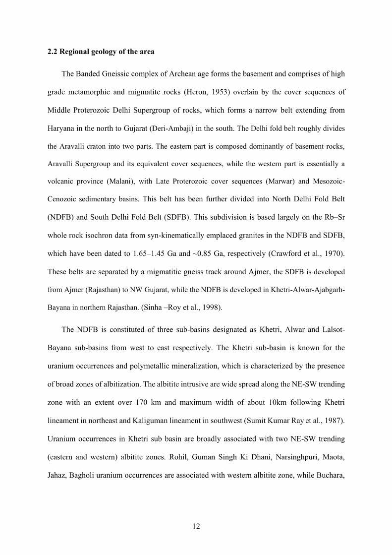
The NDFB is constituted of three sub-basins designated as Khetri, Alwar and Lalsot-
Bayana sub-basins from west to east respectively. The Khetri sub-basin is known for the
uranium occurrences and polymetallic mineralization, which is characterized by the presence
of broad zones of albitization. The albitite intrusive are wide spread along the NE-SW trending
zone with an extent over 170 km and maximum width of about 10km following Khetri
lineament in northeast and Kaliguman lineament in southwest (Sumit Kumar Ray et al., 1987).
Uranium occurrences in Khetri sub basin are broadly associated with two NE-SW trending
(eastern and western) albitite zones. Rohil, Guman Singh Ki Dhani, Narsinghpuri, Maota,
Jahaz, Bagholi uranium occurrences are associated with western albitite zone, while Buchara,
13
Ladi Ka Bas, Geratiyon Ki Dhani, Kalatopri, Rela-Ghasipura are associated with eastern
albitite zone (Kamlesh Kumar et al., 2018).
The present area of study forms the part of the Banded gneissic complex and hence it is
described in detail.
Figure 2.1 Three sub-basins of North Delhi Fold Belt, two sub-parallel albitite zone present in
the Khetri Sub-Basin and BGC (Modified after GSI,1995)
2.2.1 Banded Gneissic Complex
Banded Gneissic Complex (BGC) represents the oldest geological record in Rajasthan
and forms the basement for the Proterozoic fold belts, comprising various types of gneisses,
migmatites, high-grade schist and metabasic rocks in the gneissic terrains of Sandmata
Complex, Mangalwar Complex and the Hindoli Group. These represent the early Precambrian

14
crust formed through the process of granite-granulite greenstone accretion. Mangalwar
Complex and Hindoli Group forms greenstone type basins and result of the deformation in
oldest, elongated sedimentary basins formed in rifted ensialic crusts. Large scale acidic and
intermediate magmatic emplacements such as granite, granodiorite and tonalite plutons have
happened due to tectonic activity at about 2900 Ma. Sandmata Complex contains the high-
grade equivalent of rocks up to granulite facies. The Archaean-Proterozoic boundary in
Rajasthan is marked by a prominent phase of acid igneous activity and emplacement of Berach
Granite and equivalent granite plutons at about 2500 Ma.
2.3 Detailed geology of the study area
The study area is in and around Chhota Udaipur village, Ajmer district, Rajasthan and
it is partially soil covered and is located in the SW continuity of albitite line. It is a part of
Sandmata complex of Archaean age (2500 Ma). The western boundary is marked by the Delhi
Supergroup which overlies the Sandmata Complex along tectonised unconformity, kaliguman
lineament which separates the BGC from Delhi group of rocks and has the eastern boundary
with the Mangalwar Complex. The study area contains rocks of Badnor and Shambhugarh
Formations of Sandmata Complex and Gyangarh-Asind acidic igneous intrusive rocks of
granitic to granodioritic in composition.
The Sandmata complex is represented by biotite schist, gneisses and older mafic enclaves
comprising pyroxenite, amphibolite, hornblende schist, chlorite schist and epidiorite of Badnor
formations and migmatites and gneisses of Shambugarh formation. The uraniferous
polymetallic veins have been reported in Sandmata complex intruded by Gyangarh Asind
acidic igneous suite at two dug wells of Chhota Udaipur area, Ajmer district, Rajasthan. These
two dug wells are separated by 210m in NE-SW direction and indicates the possible subsurface
strike continuity towards the south-west of Chhota-Udaipur area.
15
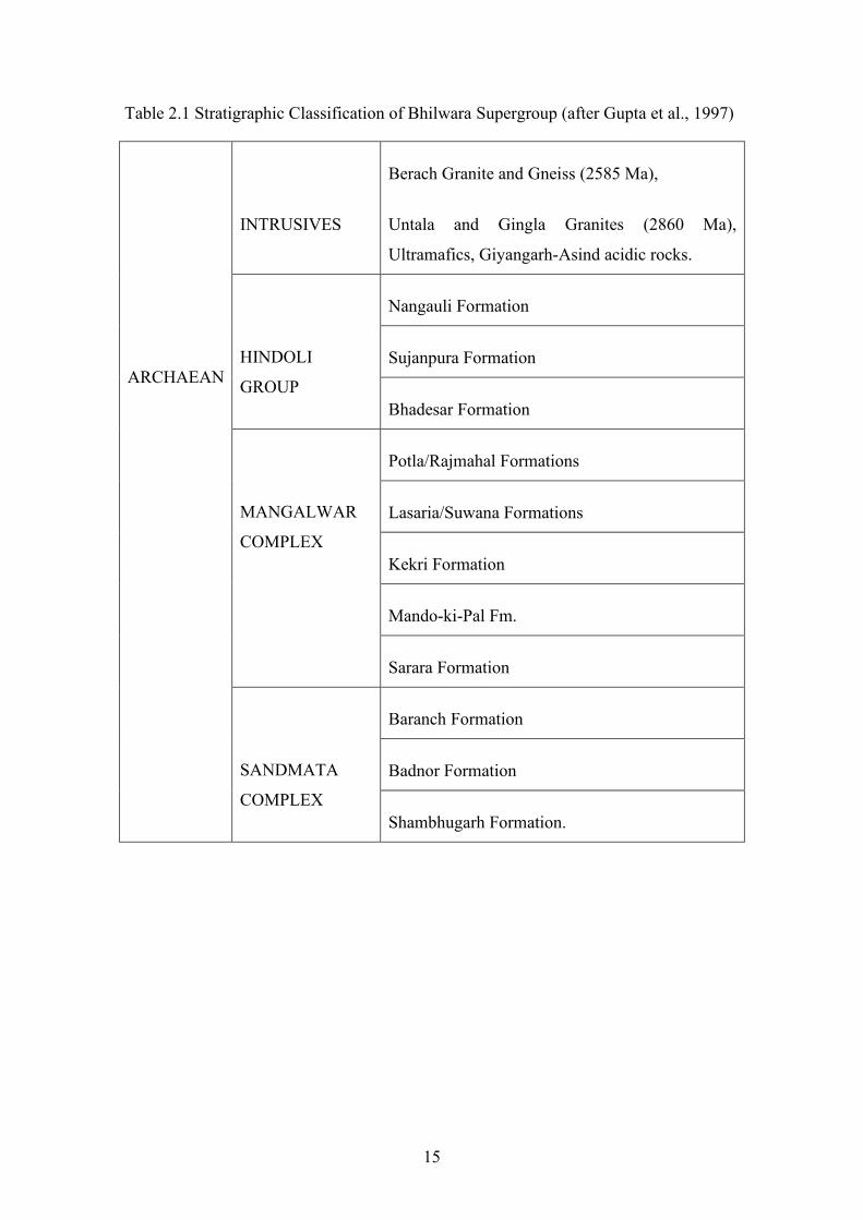
Table 2.1 Stratigraphic Classification of Bhilwara Supergroup (after Gupta et al., 1997)
ARCHAEAN
INTRUSIVES
Berach Granite and Gneiss (2585 Ma),
Untala and Gingla Granites (2860 Ma),
Ultramafics, Giyangarh-Asind acidic rocks.
HINDOLI
GROUP
Nangauli Formation
Sujanpura Formation
Bhadesar Formation
MANGALWAR
COMPLEX
Potla/Rajmahal Formations
Lasaria/Suwana Formations
Kekri Formation
Mando-ki-Pal Fm.
Sarara Formation
SANDMATA
COMPLEX
Baranch Formation
Badnor Formation
Shambhugarh Formation.

16
Figure 2.2 Geological map of Tilonia-Nasirabad area, Ajmer district, Rajasthan (modified
after Sinha et al., 2002)
KUHIL
KHATOLI
TILONIA
PATAN
Kishangarh
BANEWARIKANAKHERI
SRINAGAR
Tikawara
SURSARA
U-Mo-Cu Location
740 301 750 001
740 451
260
301
Chhota Udaipur
Naulakha Formation of Alwar group
Srinagar Formation of Alwar group
Ajmer Formation of Ajabgarh group
Nepheline and soda syenite
INDEX
Study area
Shambhugarh Formation
Gyangarh Asind acidic igneous suite
Badnor Formations
17
CHAPTER 3
MAGNETIC METHOD OF EXPLORATION
3.0 Introduction
Magnetic method is the oldest and passive geophysical method. It was developed for
mineral exploration, primarily for iron ore searching and it is one of the most widely used
geophysical method in exploration programme as a reconnaissance tool to understand the
subsurface structural features (Paterson and Reeves, 1985) which is relatively cost-effective
technique and rapid to employ. The method is based on the measurement of the lateral
variations in magnetic field which are magnetic expressions of the subsurface geological
features. For successful application of magnetic method, lateral variation in the magnetic
susceptibility is essential. Magnetic susceptibility of rocks varies with the variations in the
concentration of magnetite and other ferro, ferri-magnetic minerals in crustal rocks formed
below the Curie point temperature. As temperature increases, thermal energy begins to
breakdown the ordering of a ferromagnetic material and above the Curie temperature,
spontaneous magnetization ceases. Since temperature in the Earth increases with depth, there
exists a depth below which materials cannot behave as ferromagnetic. Thus, only rocks at
shallow depths (approximately less than 20km) in the Earth can exhibit remnant magnetization
which is a permanent magnetism of rock acquired when it was formed, in the direction of the
earth’s magnetic field at that time. So, the local magnetic anomalies are arising from variation
in magnetization contrast of crustal rocks which reflects the subsurface lithology and structural
fabric. In general, igneous and metamorphic rocks have higher magnetic susceptibilities as
compared to sedimentary rocks, the subsurface geological structures and lithological contacts,
such as basic dyke intrusives with high susceptibilities (Roberts and Smith, 1994) and
prominent fault and fractured zones with low susceptibilities, can be usefully picked up (Clark
et al., 1992; Henkel and Guzman et al., 1977; Cull and Massi et a.l, 2002 and Lopez-Loera et

18
al., 2010; Ramesh Babu et al., 2007; Srinivasa Rao et al., 2016; Vijay Kumar et al., 2015). As
such, to acquire precise subsurface information and to resolve the ambiguity in potential field
interpretation, magnetic surveys are to be followed by other geophysical methods like gravity
electrical resistivity, electromagnetic or seismic survey.
3.1 Theory of magnetic method
Geomagnetic field has different physical origins and can be found both below (in the
form of electrical currents and magnetized material) and above the Earth’s surface. Each
source happens to produce a contribution with rather specific spatiotemporal properties. The
crustal rocks are too weak to produce the observed magnetic field in the absence of external
field and mantle rocks also existed at high temperature environment so their contribution could
be nominal. According to dynamo theory earths main magnetic field is generated and
maintained by system of electrical currents in outer core,which are generated by the motion of
the conducting fluids (Radhakrishna murthy et al; 1978).
In principle, magnetic method has the ability of greater depth of investigation, thereby
magnetic surveys give 3D geological information. The fundamental non-uniqueness of
potential field source distribution is a crucial limitation of 3D interpretations of magnetic
surveys. By constraining models only ambiguity in source geometry can be estimated.
Magentic properties governs the reliability of magnetic models, besides that factors which
determine magnetisation, intensities and directions of the geological units in an area of
investigation are essential for solving geological ambiguity in acquiring reliable interpretation.
Ore bodies in the world such as Olympic dam(Esdale Donald et al., 2003), Ernest
Henry(Austin et al., 2019) of Australia and Bayon Obo (Hong et al., 2016) of China associated
with iron oxide related mineralisation were identified by using magnetic method and also
corridor of likely mineralisation delineated by mapping of the structures using magnetic
method.

19
3.2 Instruments
Two GEM make (http://www.gemsys.ca/versatile-proton-magnetometer) Proton
Precision Magnetometers (PPM) were used in the magnetic survey, one for recording the
diurnal variations at base and the other for field use as a rover. PPM measures the Earth’s
magnetic field independent of its direction to a resolution of 0.01 nT and with an accuracy of
± 0.2 nT.
Figure 3.1 GEM Systems, GSM 19T Proton Precision Magnetometer used for Data
Acquisition in the survey area (www.gemsys.ca)
PPM is a light-weight, less cumbersome equipment having a sensor, console and GPS
antenna. It can be operated in three operating modes, Walking, Mobile, and Base. These
magnetometers are integrated with inbuilt Global positioning system (GPS) receiver for
recording spatial locations along with magnetic data. Spatial horizontal accuracy of GPS is 0.6
m. It has inbuilt memory of 20 Mb to store the acquired data.

20
3.3 Magnetic Data Acquisition
Magnetic data was acquired at the station interval 25 m and traverse spacing of 100 m
and 200 m as shown in the Figure3.2.
Figure 3.2 Magnetic profile layout map, Chhota Udaipur area, Ajmer district, Rajasthan
Geological features have a NE-SW trend hence, east-west traverses were selected based
on the accessibility of the study area (Figure3.2). Total of 30 sq. km area was covered in and
around the Chhota Udaipur area with the above specified survey parameters. Diurnal variation
of the Earth’s magnetic field was recorded at every 60 seconds using a base station established
500 0 500 1000
(meters)WGS 84 / UTM zone 43N
2928000
2929000
2930000
2931000
2932000
2933000
2928000
2929000
2930000
2931000
2932000
2933000
483000 484000 485000 486000 487000 488000 489000
483000 484000 485000 486000 487000 488000 489000
26°2
8'
26°2
9'
26°3
0'
26°3
1'
26°2
8'
26°2
9'
26°3
0'
26°3
1'
74°50' 74°51' 74°52' 74°53'
74°50' 74°51' 74°52' 74°53'
Chhota Udaipur
Kumhariya Bera
Gudiyana
Tikawara
RW1
RW2
Kaliguman lineamentMagnetic data locations

21
in the cultural noise free and low magnetic gradients in the area near Chhota Udaipur village
(486384N, 293200E).
3.4 Physical property measurement
For geological mapping and geophysical prospecting, information about physical
properties of rocks are important for a plausible geological interpretation. The ultimate result
of any geophysical survey is to interpret the anomaly in terms of the geology. The magnetic
susceptibility of rocks in the study area are helpful to the interpretation of magnetic data. The
induced magnetization in a material when placed in external magnetic field depends on its
magnetic susceptibility. Susceptibility is defined as the ratio of magnetization (M) to
magnetizing field (H), given as
𝐌 = 𝐤𝐇 𝐨𝐫 𝐤 =𝐌
𝐇 ……..…. (3.1)
The units of M and H are same and hence k is dimensionless. Measurement of magnetic
susceptibility(K) helps to understand the magnetic nature of the geological formations and in
the modeling of the anomaly.
Magnetic susceptibility is measured using the portable handheld (kappa) KT-10 v2
susceptibility meter (https://www.yumpu.com/user/terraplus.ca). The instrument is working
based on the fact that the alternating magnetic field produced by Helmholtz coil induces a
magnetic field in the specimen which is proportional to the rate of change of its magnetic
moment. Knowing the magnetic field and the volume of the specimen, its susceptibility is
calculated. Measured susceptibility values are shown in table 3.1.

22
Table 3.1 Physical properties of various rock samples from Chhota Udaipur, Ajmer district, Rajasthan
S. No Rock type of the
Sample
No. of
samples
Susceptibility
(K *10-3 SI)
Radioactivity
(µR/hr)
Density
(g/cc)
1. Radioactive samples
(Magnetite bearing
Quartz biotite gneiss)
4 25 – 570 180-234 2.78
2. Quartz mica schist 4 1.9 – 2.5 11 2.84
3. Magnetite bearing
Biotite gneiss
3 25 –30 12 2.75
4. Albitized biotite gneiss 5 2.9 – 7.34 12 2.67
5. Biotite gneiss 4 0.5 – 1.5 13 2.78
6. Acidic rock
(Granodiorite)
4 0.02 – 0.03 10 2.62
7. Quartzo-felspathic rock 4 0.01 – 0.04 10 2.62
8. Hornblende gneiss 5 3 – 10 10 2.76
9. Pure Quartz vein 3 0.041-0.004 ----- 2.63
3.5 Magnetic Data processing
Geophysical data processing is the most important step and which is an intermediate
stage between data acquisition and interpretation of the data. The aim of the data processing is
to enhance the data quality by suppressing or removing the different noise present in the data.
During processing, the observed data are corrected for natural and instrumental variations.
Ground magnetic data processing includes corrections for diurnal variations of the geomagnetic
field, single spike reading, and IGRF (International Geomagnetic Reference Field) correction
to remove background/normal geomagnetic field. IGRF correction is important correction in
airborne as well as ship born magnetic surveys. However, in a limited area the

23
background/normal magnetic field variation is very less and insignificant; hence IGRF
correction is not required in detailed/semi-detailed ground magnetic surveys.
3.5.1 Diurnal correction
Diurnal variations are subject to amplitude and phase changes, depending on the geographic
location of the observer. The variations earth’s magnetic field are recorded by a base station
magnetometer located in the survey area. The measured magnetic field by using rover
magnetometer is then corrected for the diurnal variation through a direct subtraction of field
data from the corresponding time synchronized base magnetic data using GEM link software.
Variations in the geomagnetic field due to magnetic storms can be so rapid, unpredictable, and
of such large amplitude. Magnetic surveying is suspended under these conditions. The
amplitude of the diurnal variations of geomagnetic field in solar quite day is 10-30 nT and
during magnetic storms is up to 1000nT (William Lowerie, 2007). Figure 3.3 represents the
diurnal variations that of recorded by base magnetometer on a typical day during the survey
and variation of 14.3 nT was observed.
Figure 3.3 Diurnal variation of geomagnetic field on 17th December 2019
46804
46806
46808
46810
46812
46814
46816
46818
46820
46822
08:38:24 09:50:24 11:02:24 12:14:24 13:26:24 14:38:24
Ma
gn
eti
c F
ield
(n
T)
Time(GMT HR:MM:SS)
Amplitude = 14.3 nT

24
3.5.2 Correction for cultural noise
Magnetic anomalies caused by man-made features are defined as cultural noise in
magnetic survey. Cultural noise interferes with the magnetic anomalies of interest arising from
subsurface. The sources of cultural noise are ferrous objects such as drill holes lined with steel
casing, steel buildings, pipelines, bridges, tank farms, metallic fencing, power lines etc.
Generally cultural noise has high frequency (short wavelength). There is no method to
completely eliminate the cultural noise from the observed magnetic anomalies but frequency
domain techniques can suppress this noise to some extent.
In the present study, the base station has been established in such a way to avoid cultural
noise as far as possible. The observed profile data also has been thoroughly checked and single
peaks, point anomalies caused by the cultural noise are filtered. Further, fourth difference of
the anomalies has been calculated and a non-linear filter is applied to smoothen the data.
3.5.3 Data visualization
After applying all the corrections to the raw data which are mentioned above, the data
was gridded using minimum curvature gridding method with a cell size of 30 m. Minimum
curvature gridding method (Briggs, 1974) is a very popular gridding algorithm and it takes into
account surface of minimum curvature. The results are presented in the form of shaded relief
images map for better visualization. The gridded data are used for further processing and
matched filtering using frequency domain through Fourier Transform. For effective
interpretation of the acquired magnetic data, further data enhancement techniques are applied
using various transformations such as; upward continuation, reduced to pole and derivatives.
3.5.4 Filtering techniques
The initial stage of magnetic data interpretation generally involves the application of
mathematical filters to processed data with an objective to enhance anomalies of interest and
to gain some preliminary information on source location.

25
Different mathematical filtering techniques have been applied on the gridded data to
enhance the information of interest Most of the filtering techniques are mathematically more
complex to apply in time/space domain, but these techniques having simple mathematical
operations in frequency domain. Filtering operations in frequency domain improves the
efficiency of the filter and decreases the run time. Hence, Fourier transformation is used to
transform the data into frequency/wavenumber domain. After applying filtering technique in
frequency domain, this data is transformed back into time/wavelength domain using inverse
Fourier transformation.
3.6 Interpretation of Magnetic Data
The magnetic anomaly of a finite body invariably contains positive and negative
anomalies arising from the bipolar nature of magnetism. Magnetic interpretation is classified
as qualitative interpretation and quantitative interpretation methods. The aim of the qualitative
interpretation is a visual inspection of the shape and trend of the magnetic anomalies such as
sharpness of anomalies, elongation and areal extends of the contours, +ve and -ve peaks of the
anomalies to delineate the strike of the formations, structural trends, and regional tectonics.
Generally, in contoured maps, when the lines are close together, they represent a steep gradient
and high-density contours indicates litho-contact, faults/fractures. When contour lines are
widely spaced, they represent shallow gradient or slow change in magnetic value. Closed
contours are associated with three-dimensional body in the subsurface, while the elongated
contour indicates two-dimensional body with strike along the contours trend. The breaks and
offset in the contours also a key feature in the identification of faults/fractures. Quantitative
interpretation includes estimation of depth to the top of the source body, 2D/3D profile
modelling and Inversion. Interpretation is ambiguous even in the case of high-quality data
because the observed anomaly can be replicated by an infinite number of source distributions
shallower or possibly deeper than the actual source of the anomaly and moreover potential field

26
measured at the surface can be considered as integral of potential fields from all depth. There
is no depth control in potential fields and it is up to center of the Earth in case of gravity and
up to Curie’s temperature in case of magnetics. The ambiguity is not relieved by additional
measurements of the magnetic field and its various components or by observations at different
levels, because these are not independent measurements. Thus, geological information,
borehole information and/or other geophysical data is required for the successful interpretation
of magnetic anomalies.
3.6.1 Qualitative interpretation
3.6.1.1Total Magnetic Intensity Anomaly Map
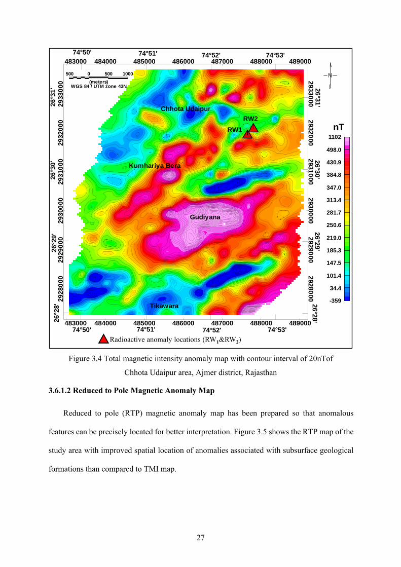
Total magnetic intensity (TMI) anomaly map (Figure 3.4) has been prepared by
applying minimum curvature gridding technique with a 30 m cell size using Geosoft software
(http://www.geosoft.com). The amplitude of TMI anomaly varies from -359 nT to 1102 nT.
The contour pattern of the anomaly indicates the general trend of geological features in the
study area as NE-SW direction. Two strong bipolar magnetic signatures have been observed
towards central and south-eastern part of study area indicating the presence of ENE-WSW
trending high magnetic bodies. Interpretation on TMI map for structural features and litho-
contacts is complex because of the bipolar nature of the magnetic field. In order to remove the
inclination (41.682o) and declination (1.07o) effects of Earth’s magnetic field, reduced to pole
(RTP) filter was used.
27
Figure 3.4 Total magnetic intensity anomaly map with contour interval of 20nTof
Chhota Udaipur area, Ajmer district, Rajasthan
3.6.1.2 Reduced to Pole Magnetic Anomaly Map
Reduced to pole (RTP) magnetic anomaly map has been prepared so that anomalous
features can be precisely located for better interpretation. Figure 3.5 shows the RTP map of the
study area with improved spatial location of anomalies associated with subsurface geological
formations than compared to TMI map.
500 0 500 1000
(meters)WGS 84 / UTM zone 43N
2928
000
2929
000
29300
00
2931
000
29320
00
2933
000
2928
000
2929
000
29300
00
2931
000
29320
00
2933
000
483000 484000 485000 486000 487000 488000 489000
483000 484000 485000 486000 487000 488000 48900026
°28'
26°2
9'
26
°30'
26°3
1'
26°2
8'
26°2
9'
26°3
0'
26
°31'
74°50' 74°51' 74°52' 74°53'
74°50' 74°51' 74°52' 74°53'
Chhota Udaipur
Kumhariya Bera
Gudiyana
Tikawara
RW1
RW2
Radioactive anomaly locations (RW1&RW2)
500 0 500 1000
(meters)WGS 84 / UTM zone 43N
-359
1102
34.4
101.4
147.5
185.3
219.0
250.6
281.7
313.4
347.0
384.8
430.9
498.0
nT
2928000
2929000
2930000
2931000
2932000
2933000
2928000
2929000
2930000
2931000
2932000
2933000
483000 484000 485000 486000 487000 488000 489000
483000 484000 485000 486000 487000 488000 489000
26°2
8'
26°2
9'
26°3
0'
26°3
1'
26°2
8'
26°2
9'
26°3
0'
26°3
1'
74°50' 74°51' 74°52' 74°53'
74°50' 74°51' 74°52' 74°53'
Chhota Udaipur
Kumhariya Bera
Gudiyana
Tikawara
RW1
RW2
20
02
20
20
02
20
1 4 0
1 40
04
1
041
140
1 4 0
14
0
04
1
1 4 0
04
1
14
0
04
1
04
1
041
140
1 4 0
04
1
0411 4 0
14
0
04
1
14
0
2 2 0
022
02
2
02
2
2 2 0
022
022
22
0
02
2
02
2
02222
0
02
2
2 20
022
02
2
2 2 0
02
2
02
2
022
26
0
26
0
2 60
062
06
2
062
062
26
0
26
0
26
0
06
2
2 60
26
0
2 60
062
0620
62
2 6 0
2 60
062
26
0
062
2 60
34
0
3 4 0
34
0
3 40
34
0
04
334
0
340
04
3
3 4 0
3 4 0
3 40
3 4 0
04
3
34
0
3 40
340
043043
3 80
08
3
38
0
38
0
08
3
3 8 0
38
0
380
08
3
3 8 0
3 8 0
08
338
0
380
08
3
08
3
083
46
0
064
46
0
460
58 0
02
6
04
7
8 6 0

28
Figure 3.5 Reduced to pole anomaly map, Chhota Udaipur area, Ajmer district, Rajasthan
The trend and disposition of magnetic anomaly sources are clearly demarcated in reduced
to pole map as shown in Figure3.5. Based on variation in anomaly trend and amplitude,
prominent NE-SW, E-W and NW-SE trending subsurface fault/fractures have been delineated
in the study area. The low magnetic signature L1 observed in the north western part of the map
is because of the presence of low susceptibility quartz-mica-schist and it is observed that the
strike of the formation changes from NE-SW to ENE-WSW direction. The moderate low
500 0 500 1000
(meters)WGS 84 / UTM zone 43N
-289
1126
36
88
122
150
179
207
245
286
337
406
481
610
nT
29
28
00
02
92
90
00
29
30
00
02
93
10
00
29
32
00
02
93
30
00
29
28
00
02
92
90
00
29
30
00
02
93
10
00
29
32
00
02
93
30
00
483000 484000 485000 486000 487000 488000 489000
483000 484000 485000 486000 487000 488000 48900026
°28
'26
°29
'26
°30
'26
°31
'
26
°28
'26
°29
'26
°30
'26
°31
'
74°50' 74°51' 74°52' 74°53'
74°50' 74°51' 74°52' 74°53'
Chhota Udaipur
Kumhariya Bera
Gudiyana
Tikawara
RW1
RW2
Inferred fault/fracturesLitho contact
Radioactive anomaly locations (RW1, RW2)
H1, H2 and H3 > 400 nT; High magnetic signaturesL1, L2 and L3 < 180 nT; Low magnetic signatures
L1
L2
L3
H1
H2
H3

29
magnetic signature L2 in the eastern side of study area is attributed to the country rock
hornblende gneiss. The very low magnetic signature L3 towards the southern side of the
Gudiyana village may interpreted as injection of the Gyangarh Asind acidic igneous intrusives
within BGC.
The previously reported Chhota Udaipur radioactive anomaly is associated with the
moderate high magnetic (>460 nT on RTP map) signature. The high magnetic signature H1(>
400 nT) near kumariya bera village, is due to the presence of magnetite bearing biotite gneiss.
The high magnetic signatures H2, H3 in the center and south-eastern part of the study area are
possibly due to the mafic intrusives (Pyroxenite’s) of Badnor formation or association of gneiss
with magnetite mineralisation, since there is no rock exposure in this area to certainly attribute
to magnetic anomaly. Many small spatially limited magnetic anomalies with relatively moderate
amplitude have been observed in the north and eastern side of the study area, which could be due
to polymetallic injections in BGC.
3.6.1.3 Upward continuation filter
Upward continuation is a mathematical technique that project data taken at an elevation
to a higher elevation. The effect is that short wavelength features are smoothed out because
one is moving away from the anomaly (Radhakrishna murthy et al., 1978). Upward
continuation is a way of enhancing large scale (usually deep) features in the survey area and
tends to accentuate anomalies caused by deep sources at the expense of anomalies caused by
shallow sources.
Upward continuation filter has been applied to the RTP grid at 400 m level of height. As stated
earlier several small magnetic anomalies with relatively moderate amplitude in the north and eastern side
of the study area (Figure 3.5) are attenuated in 400m upward continued map which indicates that the
anomalies have originated from shallow sources. The prominent the high magnetic signatures H1, H2, H3

30
in the study area showing strong high amplitudes even at 400m (Figure 3.6) and above continued heights
which indicating that these high magnetic bodies have greater depth extension in the BGC.
Figure 3.6 Upward continued magnetic (RTP) map of 400m level, Chhota Udaipur area,
Ajmer district, Rajasthan
3.6.1.4 First Vertical Derivative Filter
First Vertical Derivative (FVD) is the first order differentiation of observed anomalies
with depth which emphasizes the contributions from shallow sources at the expense of those
from the larger and deep-seated sources. It is also used to sharpen the shallow contacts and
500 0 500 1000
(meters)WGS 84 / UTM zone 43N
107
536
137
178
206
229
249
268
287
306
327
350
378
418
nT
2928000
2929000
2930000
2931000
2932000
2933000
2928000
2929000
2930000
2931000
2932000
2933000
483000 484000 485000 486000 487000 488000 489000
483000 484000 485000 486000 487000 488000 489000
26°2
8'
26°2
9'
26°3
0'
26°3
1'
26°2
8'
26°2
9'
26°3
0'
26°3
1'
74°50' 74°51' 74°52' 74°53'
74°50' 74°51' 74°52' 74°53'
Chhota Udaipur
Kumhariya Bera
Gudiyana
Tikawara
RW1
RW2
30
0
30
0
40
0
4 0 0
40
0
H2
H1
H3
Trend of the high magnetic bodies

31
structural features (Telford et al., 1990; Lowrie et al., 2007; Radhakrishna murthy et al., 1978).
FVD filter has been applied over RTP grid.
Figure 3.7 FVD of RTP anomaly map, Chhota Udaipur area, Ajmer district, Rajasthan
From the FVD filtered map (Figure 3.7), it has been observed that the high magnetic
anomalies are enhanced and closely-spaced anomalies are better resolved. Based on variation
in anomaly trend and amplitude, prominent subsurface structural features trending NE-SW, E-
W and NW-SE fault/fractures have been demarcated in the study area as shown in Figure 3.7.
500 0 500 1000
(meters)WGS 84 / UTM zone 43N
-2.29
3.23
-0.70
-0.48
-0.36
-0.26
-0.18
-0.11
-0.03
0.05
0.17
0.32
0.51
0.83
nT/m
2928
000
29290
00
2930
000
2931
000
29320
00
29330
00
2928
000
2929
000
2930
000
29310
00
2932
000
29330
00
483000 484000 485000 486000 487000 488000 489000
483000 484000 485000 486000 487000 488000 489000
26
°28'
26°2
9'
26
°30'
26°3
1'
26°2
8'
26°2
9'
26°3
0'
26°3
1'
74°50' 74°51' 74°52' 74°53'
74°50' 74°51' 74°52' 74°53'
Chhota Udaipur
Kumhariya Bera
Gudiyana
Tikawara
RW1RW2
Inferred fault/fractures

32
3.6.1.5 Tilt Derivative or Tilt angle method
Tilt Derivative (TDR) method proposed by Salem et al. (2008) has come into wide use
as an aid for interpreting magnetic gridded data. High TDR values are commonly associated
with lateral contrasts in magnetization and may represents dikes. The low TDR values may
represent nonmagnetic or alteration zones, fractures or faults within the country rock. The tilt
angle technique is the ratio of the vertical derivative to absolute value of the total horizontal
derivative of the magnetic field
TDR_Ɵ = tan−1 (∂T
∂z______|THDR|
) ……. (3.2)
Where T is the total magnetic field, ∂T
∂z is the vertical derivative of the magnetic field
|THDR =∂T
∂x+
∂T
∂y| absolute value of the total horizontal derivative of the magnetic field
The tilt angle amplitudes are restricted to values between –π/2 and +π/2; thus, the
method limits the amplitude variations into a certain range therefore it functions like an
automatic-gain-control filter which responds equally well to shallow and deep sources. The
amplitude of the tilt angle is positive over the magnetic sources, crosses through zero at or near
the edge of the source, and is negative outside the source (Miller and Singh, 199; Salem et al
2007). The half-distance between +450 and -450 contours provide an estimate of the source
depth for vertical contacts. Tilt derivative map of the study area clearly demarcated the contacts
between high magnetic and low magnetic bodies with zero (radians) contour and also brought
out prominent NE-SW, NW-SE and east west fracture zones in the survey area as shown in
Figure 3.8. Low TDR values have been observed towards the southern portion of the study
area, which could be due to the alteration of gneissic rocks by the intrusion of Gyangarh Asind
acidic igneous rocks. The depth to sources are estimated from tilt angle technique, the high
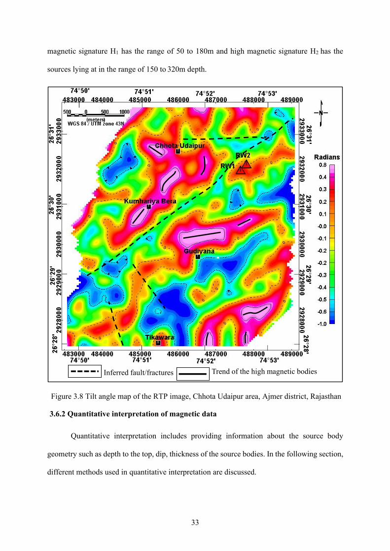
33
magnetic signature H1 has the range of 50 to 180m and high magnetic signature H2 has the
sources lying at in the range of 150 to 320m depth.
Figure 3.8 Tilt angle map of the RTP image, Chhota Udaipur area, Ajmer district, Rajasthan
3.6.2 Quantitative interpretation of magnetic data
Quantitative interpretation includes providing information about the source body
geometry such as depth to the top, dip, thickness of the source bodies. In the following section,
different methods used in quantitative interpretation are discussed.
Inferred fault/fractures Trend of the high magnetic bodies

34
3.6.2.1 Euler deconvolution
Thompson et al.,1982 proposed a technique for analysing magnetic data based on
Euler relation for homogeneous functions. The Euler deconvolution technique uses first-order
x, y, and z derivatives to determine location and depth for various idealized targets (sphere,
cylinder, thin dike, contact), each characterized by a specific structural index (SI). A structural
index is an exponential factor corresponding to the rate at which the field falls off with distance,
for a source of a given geometry. SI for different source geometries are as follows
SI Source geometry
0 Contact / Step
1 Sill / Dyke
2 Cylinder / Pipe
3 Sphere
Although theoretically the technique is applicable only to a few body types which have a known
constant structural index, the method is applicable in principle to all body types. Reid et al.,
(1990) extended the technique to 3D data by applying the Euler operator to windows of gridded
data sets. The Euler deconvolution technique is insensitive to magnetic inclination, declination
and remanence.
In this study, the Euler deconvolution technique was applied over the TMI grid for
location and depth determination of causative anomalous bodies from observed magnetic field
data. Different structural indexes and window lengths have been tested for cluster of Euler
solutions, eventually structural index SI=0 where Window of 10 x 10m data points proved to
be most suitable and is used for depth estimation.

35
Figure 3.9 Euler solutions over TMI map, Chhota Udaipur area, Ajmer district, Rajasthan
The minimum and maximum source depth ranges obtained by this method are 50 m to 350 m
and solutions with depths to source above the error tolerance levels are rejected. These solutions
are plotted over TMI map as shown in Figure3.9. The center of the plotted circles represents the
location (x0 &y0) of the interpreted source. Similarly, depths are displayed using color variation
to represent 4 different ranges. From the figure, it is observed that in the northern part of the
study area depth solutions are predominantly shallower(<50m) to intermediate (50 m-100 m)
and contacts near earlier reported radioactive anomalies are giving depth solutions in this range.
The solutions for relatively deeper depths from 100m to 200m and more are located in the
western and southern part of the study area. It is also observed that the high magnetic signature
500 0 500 1000
(meters)WGS 84 / UTM zone 43N
(m)Depth
< 5050 - 100
100 - 200> 200
-359
1102
34.4
101.4
147.5
185.3
219.0
250.6
281.7
313.4
347.0
384.8
430.9
498.0
nT
29
28
00
02
92
90
00
29
30
00
02
93
10
00
29
32
00
02
93
30
00
29
28
00
02
92
90
00
29
30
00
02
93
10
00
29
32
00
02
93
30
00
483000 484000 485000 486000 487000 488000 489000
483000 484000 485000 486000 487000 488000 4890002
6°2
8'
26
°29
'2
6°3
0'
26
°31
'
26
°28
'2
6°2
9'
26
°30
'2
6°3
1'
74°50' 74°51' 74°52' 74°53'
74°50' 74°51' 74°52' 74°53'
Chhota Udaipur
Kumhariya Bera
Gudiyana
Tikawara
RW1
RW2

36
H2 is associated with deeper depth solutions than compared with that of high magnetic
signature H1. It is observed from Figure 3.9 that the Euler solutions clearly indicate the
magnetic sources are relatively shallower in the northern portion of the study area than
compared to the southern side.
3.6.3 Modeling and Inversion of Magnetic Data
Modeling and inversion refers to the assumption of geophysical models and parameters
based on known geology and modifying in an iterative approach such that the observed
anomalies and theoretical anomalies fit closely. All the inversion schemes are iterative and
utilize one or the other form of optimization techniques. Quantitative interpretation refers to
drawing geologic conclusions from the inverted models. As is typical for geophysical inverse
problems, a purely mathematical solution of magnetic inversion is nonunique. In inversion, a
model is parameterized to describe either source geometry or the distribution of a physical
property such as magnetic susceptibility.
3.6.3.1 2-D Forward Modeling
Forward modeling refers to the computation of theoretical magnetic anomalies for assumed
geometry and shape parameters which is useful in understanding the magnetic anomalies in
terms of subsurface geology. Two dimensional (2D) forward modeling studies have been
carried out using GM-SYS module of Oasis Montaj software along a representative profile
‘AB’ (Figure3.10). This profile has been extracted from TMI grid in the NNW-SSE direction
in such way to represent all the major litho-units in the study area. Results from Euler depth
solutions and susceptibility values measured from different geological rock units have been
utilized as input and the ambiguity in the modeling of magnetic data has been minimized.

37
Figure 3.10 Profile AB over TMI map for 2D modeling
500 0 500 1000
(meters)WGS 84 / UTM zone 43N
-359
1102
34.4
101.4
147.5
185.3
219.0
250.6
281.7
313.4
347.0
384.8
430.9
498.0
nT
29
28
00
02
92
90
00
29
30
00
02
93
10
00
29
32
00
02
93
30
00
29
28
00
02
92
90
00
29
30
00
02
93
10
00
29
32
00
02
93
30
00
483000 484000 485000 486000 487000 488000 489000
483000 484000 485000 486000 487000 488000 4890002
6°2
8'
26
°29
'2
6°3
0'
26
°31
'
26
°28
'2
6°2
9'
26
°30
'2
6°3
1'
74°50' 74°51' 74°52' 74°53'
74°50' 74°51' 74°52' 74°53'
Chhota Udaipur
Kumhariya Bera
Gudiyana
Tikawara
RW1
RW2
B
A

38
Figure 3.11 2D geological model of profile AB, Chhota Udaipur area, Ajmer district, Rajasthan
39
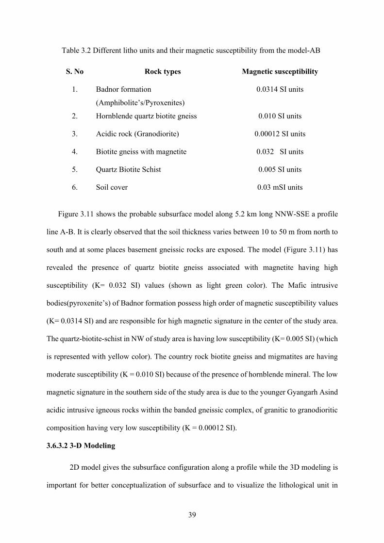
Table 3.2 Different litho units and their magnetic susceptibility from the model-AB
S. No Rock types Magnetic susceptibility
1. Badnor formation
(Amphibolite’s/Pyroxenites)
0.0314 SI units
2. Hornblende quartz biotite gneiss 0.010 SI units
3. Acidic rock (Granodiorite) 0.00012 SI units
4. Biotite gneiss with magnetite 0.032 SI units
5. Quartz Biotite Schist 0.005 SI units
6. Soil cover 0.03 mSI units
Figure 3.11 shows the probable subsurface model along 5.2 km long NNW-SSE a profile
line A-B. It is clearly observed that the soil thickness varies between 10 to 50 m from north to
south and at some places basement gneissic rocks are exposed. The model (Figure 3.11) has
revealed the presence of quartz biotite gneiss associated with magnetite having high
susceptibility (K= 0.032 SI) values (shown as light green color). The Mafic intrusive
bodies(pyroxenite’s) of Badnor formation possess high order of magnetic susceptibility values
(K= 0.0314 SI) and are responsible for high magnetic signature in the center of the study area.
The quartz-biotite-schist in NW of study area is having low susceptibility (K= 0.005 SI) (which
is represented with yellow color). The country rock biotite gneiss and migmatites are having
moderate susceptibility (K = 0.010 SI) because of the presence of hornblende mineral. The low
magnetic signature in the southern side of the study area is due to the younger Gyangarh Asind
acidic intrusive igneous rocks within the banded gneissic complex, of granitic to granodioritic
composition having very low susceptibility (K = 0.00012 SI).
3.6.3.2 3-D Modeling
2D model gives the subsurface configuration along a profile while the 3D modeling is
important for better conceptualization of subsurface and to visualize the lithological unit in

40
three dimensional (3D). 3D modeling of magnetic data provides 3D distribution of magnetic
susceptibility in the subsurface. To allow maximum flexibility for the model to represent it in
geologically realistic structures, we discretize the 3-D model region into a set of rectangular
cells, each having a constant susceptibility. The number of cells is generally far greater than
the number of the data available, thus problem is underdetermined which is solved by
minimizing a global objective function composed of the model objective function and data
misfit. The algorithm can incorporate a priori information into the model objective function by
using one or more appropriate weighting functions. The model for inversion of susceptibility a
positivity constraint is imposed to reduce the non-uniqueness and to maintain physical
reliability. We assume that there is no remanent magnetization and that the magnetic data are
produced by induced magnetization only while inverting the data. An attempt has been made
to invert the magnetic data using UBC MAG3D (www.eoas.ubc.ca) which resulted to the
susceptibility distribution in 3D.
Table 3.3 Inversion parameters of 3D magnetic voxel model
S. No Parameter Description Parameter value
1 Total no. of data points 5035
2 Total no. of cells in X-direction 200
3 Total no. of cells in Y-direction 102
4 Total no. of cells in Z-direction 53
5 Total no. of cells 1081200
6 Number of iterations 27
7 Sensitivity of the model Min: 4.24E-09 and Max: 3.78E-08
8 achieved relative error 8.9554E-02
Inverted 3D magnetic susceptibility distribution of magnetic data using UBC MAG3D
is shown in Figure3.12 but it was a completely mathematical model. The first order trend
(regional) has been removed from the observed magnetic data for the enhancement of residual
anomaly before doing the 3D-inversion which resulted the subtle anomalies to be more clearly

41
visible. The high magnetic signature H1 (Figure 3.5) near Chhota Udaipur village gets truncated
at places by fault/fractures and discrimination of low susceptibility NE-SW fracture are clearer
in inverted model. The high magnetic signature H2 near Gudiyana village showing
displacement in its eastern extension may be due to fault/fracturing which is not clear in RTP
map as compared to 3D inverted model. and 3D model illustrates the SW continuity high
susceptibility distribution of the magnetic anomaly H2.
Figure 3.12 3-D Inverted Magnetic model of Chhota Udaipur area, Ajmer district, Rajasthan
Magnetic susceptibility measurement of rock samples forms a basis for the interpretation about
type and nature of magnetic sources. The susceptibility of magnetite bearing biotite gneisses are
having around 30 mSI units and responsible the high magnetic signature H2(> 400nT) near
kumariya bera village. Iso surfaces of 30 mSI susceptibility have been prepared to understand
the distribution of particular susceptibility value implies the rock type and overlaid on the RTP
SI
Inferred fault/fractures
Trend of the high magnetic susceptibility bodiesEdges of the high magnetic susceptibility bodies

42
map (Figure 3.13). The iso surface of 30 mSI magnetic susceptibility representing magnetite
bearing biotite gneiss is well resolved in the depth range of 80 m to 650m and correlates with
the high magnetic signatures in RTP map.
Figure 3.13 Inverted magnetic model highlighting the high susceptibility iso-surface
(K= 30 mSI unit) overlaid on the RTP map, Chhota Udaipur area, Ajmer district, Rajasthan
Different Depth slices of magnetic susceptibility distribution at the levels 200 m, 400
m and 600 m are shown in Figure 3.14. Depth slice at 200 m indicates the presence of many
small high magnetic susceptibility sources (magnetic susceptibility > 15 mSI) in the western
and north eastern part of the survey area. Depth slice at the level of 400 m and 600 m, shows
features which are attributed to mafic bodies/ magnetite mineralisation within the gneisses of
Sandmata complex having the depth extension.
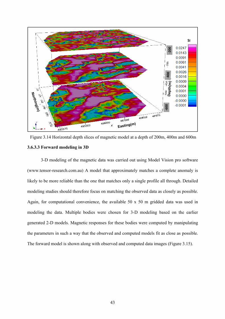
43
Figure 3.14 Horizontal depth slices of magnetic model at a depth of 200m, 400m and 600m
3.6.3.3 Forward modeling in 3D
3-D modeling of the magnetic data was carried out using Model Vision pro software
(www.tensor-research.com.au) A model that approximately matches a complete anomaly is
likely to be more reliable than the one that matches only a single profile all through. Detailed
modeling studies should therefore focus on matching the observed data as closely as possible.
Again, for computational convenience, the available 50 x 50 m gridded data was used in
modeling the data. Multiple bodies were chosen for 3-D modeling based on the earlier
generated 2-D models. Magnetic responses for these bodies were computed by manipulating
the parameters in such a way that the observed and computed models fit as close as possible.
The forward model is shown along with observed and computed data images (Figure 3.15).
SI
-20
0-6
00

44
Figure 3.15 TMI map and 3D modelled TMI response

45
The response of 3D subsurface bodies is shown in Figure 3.16. From 3D modeling it is
observed that the high magnetic source of anomaly H2 is not continuous, has irregular
distribution and high magnetic intrusive body in SW of Gudiyana village is better resolved
from these modeling studies. Apart from the three prominent high magnetic anomalies, there
are several moderate magnetic anomalies with limited spatial and depth extension which are
interpreted as polymetallic injections in BGC.
Figure 3.16 3D forward modeling for observed TMI response

46

47
CHAPTER 4
INDUCED POLARIZATION AND RESISTIVITY METHOD OF
EXPLORATION
4.1 Introduction
Resistivity survey is extensively used in mineral exploration with an objective of direct
detection of electrically anomalous targets, in particular sulphides and metal oxide
mineralization as it provides information about distribution of electrical conductivity, a
measure of the ease with which electrical currents flow within the subsurface. From the
resistivity survey we can get the information about the geometry and electrical characteristics
of the source of anomalies. The Induced Polarization (IP) survey is similar to electrical
resistivity method, is a relatively new technique in geophysics, and has been employed mainly
in base-metal exploration and to a minor extent in groundwater search (Seigel et al., 1997)
IP refers to a resistive blocking action in earth materials and the process is most
pronounced in fluid-filled pores next to metallic minerals. IP is a current-induced
electrochemical phenomenon observed as delayed voltage response in earth materials for
exploring subsurface mineral deposits. The IP effect is therefore observed to be strongest near
rocks containing metallic luster minerals (Marshall and Madden, 1959; Sumner, 1976). The IP
anomalies are mainly caused by the metallic minerals such as disseminated sulphides and
graphite or by the oxides such as magnetite (Telford, 1990). The IP phenomenon is measured
by passing a controlled inducing current through a substance and observing resultant voltage
changes with time or with variations of inducing frequency.
Field measurements of the I.P. effect may be divided into two main groups, the
frequency domain and time domain methods. In the frequency-domain methods, the dispersive
nature (or effect as a function of frequency) of the phenomenon is observed and is measured at

48
least two frequencies, for example at 1 Hz. and 10 Hz expressed as units of "percent frequency
effect" or PFE. In the time domain method, measured the decay of the potential after switching
off a d.c. current. Time domain IP has been extensively used for mapping subsurface metallic
ore bodies, environmental problems and permeability imaging (Borner et al.,1996; Oldenburg
et al., 1997).
Satyanarayana et al., 2018 effectively utilized the IP and Resistivity methods in search of base
metal exploration. Vijaya Kumar et al., 2015; Shrajala Pitla et al., 2015; Srinivasa Rao et al.,
2016 and Srinivasa Rao et al., 2018 have successfully applied the IP and Resistivity techniques
to delineate the fractures, faults, shear zones and conductive horizons for uranium exploration
in NDFB, Rajasthan.
4.2 Theory of Induced polarization
The principal cause of induced polarization in mineralized rocks is a current-induced
electron transfer reaction between electrolyte ions and metallic-luster minerals. When metallic
minerals block or are next to electrolyte-filled pore paths and an electric current flow through
the rock, an electrochemical over-potential (overvoltage) builds up at the interface between the
electron-conducting mineral and the pore solution. These electrochemical forces that oppose
current flow are described as polarizing the interface and the increase in voltage required to
drive current through the interface is called the overvoltage (Marshall and Madden, 1959;
Sumner, 1976). Even after removal of applied current, voltage does not come to zero
instantaneously it will take finite time to decay to zero. The effect of induced polarization
mainly caused by the metallic minerals such as disseminated sulphides and graphite or by the
oxides such as magnetite (Telford, 1990). The IP effect is most pronounced near rocks
containing dispersed metallic mineral grains. Polarization can increase with fluid content and
decreases with pore space. Induced polarization can be expressed relatively in percentage (%)
as the ratio of secondary voltage to applied primary voltage (Vp). Measurements are taken at a
49
number of discrete time intervals during the charge decay and stacked using repeats to improve
the signal to noise ratio. The IP effect is caused by two main mechanisms, which are membrane
polarization and the electrode polarization effects.
4.2.1 Membrane polarization
Membrane polarization is caused by presence of clay minerals and constriction within
the pore channel. The effect decreases with increasing salinity of the pore fluid. Electrolytic
conduction is the predominate factor in most rocks when no minerals are present and the
frequency is low. Most of the rock forming minerals have a net negative charge on their outer
surfaces in contact with the pore fluid and attract positive ions onto this surface from pore fluid.
The concentration of positive ions extends about 100 μm into the pore fluid, and if this distance
is of the same order as the diameter of the pore throats, the movement of ions in the fluid
resulting from the impressed voltage is inhibited (Telford, 1990). Negative and positive ions
thus build up on either side of the blockage and, on removal of the impressed voltage, return to
their original locations over a finite period of time causing a gradually decaying voltage.
4.2.2 Electrode polarization
When metallic minerals are present in a rock, an alternative, electronic path is available
for current flow. Figure 4.1(b) shows a rock in which a metallic mineral grain blocks a pore,
when a voltage is applied to either side of the pore space, positive and negative charges are
imposed on opposite sides of the grain. An electro chemical reaction takes place at the interface
between the grain surface and pore fluid. Negative and positive ions then accumulate on either
side of the grain which are attempting either to release electrons to the grain or to accept
electrons conducted through the grain. The rate at which the electrons are conducted is slower
than the rate of electron exchange with the ions. Consequently, ions accumulate on either side

50
of the grain and cause a build-up of charge. When the impressed voltage is removed the ions
slowly diffuse back to their original locations and cause a transitory decaying voltage.
Figure 4.1(A) Membrane polarization (B) Electrode polarization (after Telford et. Al., 1990)
In the present study IP data has been acquired in time domain (TDIP) mode, hence
measurement of IP response in time domain is only discussed in detail.
4.3 Measurement of Induced Polarization
IP effect is measured by injecting controlled current into the ground and measuring the
change in voltage with respect to time. When the induced current is turned off, the primary
voltage almost immediately drops to a secondary response level and then the transient voltage
diminishes with time (Figure 4.2). Measurement of the secondary voltage is one means of
measuring the polarization of a material. IP effect is normally measured in conjunction with
apparent resistivity.
There are several different ways of measuring the IP effect in the time domain. The
most commonly measured parameter is the Chargeability M, is the area (commonly in
millivolt/volt) between the decay curve over a certain time interval (t1–t2) and the zero-volt
level (Figure 4.2). This value is usually normalized by dividing it by the peak charging voltage.

51
Chargeability (M) is defined as M =∫ 𝑽𝒔
𝒕𝟐𝒕𝟏
𝑽𝒊
1
∆𝑡 ………… (4.1)
Where, Vi, Vs are the primary voltage and secondary voltages respectively.
The Figure 4.2 shows induced current waveform used in IP/Resistivity survey. Potential
difference is measured during the ON time of the current and apparent resistivity computed by
using the equation (4.3), here the decay voltage has been recorded during OFF time with pre-
programmed ON-OFF times from 0.5 to 8 seconds by factor of 2. Thus, it is operating at a base
frequency of 0.5 Hz, 0.25 Hz, 0.125 Hz, 0.0625 Hz and 0.03125 Hz with a duty cycle of 50%.
Figure 4.2 IP measurement (after Michael Dentith et al., 2014)
4.4 Theory of DC Resistivity method
The resistivity of a material is defined as the resistance between the two opposite faces
of a unit cube of the material. For a conducting cylinder of resistance 𝛿𝑅, length 𝛿𝐿 and cross-
sectional area 𝛿A (Figure 4.3) the resistivity 𝜌 is given by,

52
𝜌 =𝛿𝑅∗𝛿𝐴
𝛿𝐿 ………… (4.2)
Where, 𝜌 represents the resistivity. SI unit of resistivity is Ohm.m and the reciprocal of this is
conductivity whose unit is Siemens/m.
Figure 4.3 Schematic diagram for the resistivity(𝜌) when current passes through a cylinder
Many factors influence the resistivity of a given material which are mineral grains, fluid
content in the matrix, the degree of saturation in the pore spaces etc. The apparent resistivity
can be calculated from the measurement of potential difference between the two potential
electrodes When we injected the current into the ground through two current electrodes. For
the homogeneous and isotropic half-space, the resistivity can be calculated for any electrode
configuration. Resistivity 𝜌 for electrode arrangement as shown in Figure 4.4
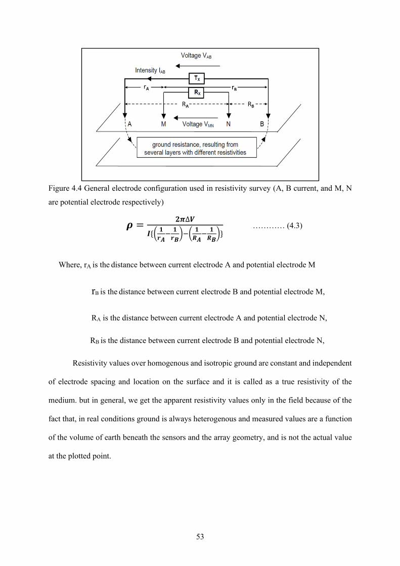
53
Figure 4.4 General electrode configuration used in resistivity survey (A, B current, and M, N
are potential electrode respectively)
𝝆 =𝟐𝝅∆𝑽
𝑰{(𝟏
𝒓𝑨−
𝟏
𝒓𝑩)−(
𝟏
𝑹𝑨−
𝟏
𝑹𝑩)}
………… (4.3)
Where, rA is the distance between current electrode A and potential electrode M
rB is the distance between current electrode B and potential electrode M,
RA is the distance between current electrode A and potential electrode N,
RB is the distance between current electrode B and potential electrode N,
Resistivity values over homogenous and isotropic ground are constant and independent
of electrode spacing and location on the surface and it is called as a true resistivity of the
medium. but in general, we get the apparent resistivity values only in the field because of the
fact that, in real conditions ground is always heterogenous and measured values are a function
of the volume of earth beneath the sensors and the array geometry, and is not the actual value
at the plotted point.

54
4.5 Data Acquisition of IP and Resistivity Data
4.5.1 Instrumentation
IP equipment of IRIS make is used for the present study (www.irisinstruments.com). The
transmitter is energized with a 3-phase voltage regulated motor generator (MG) operating at
20 kW, 220 V and 60 Hz frequency. The voltage is maintained between 180 V to 240 V. The
instrument has got several safety features to prevent damage under abnormal conditions like
unregulated or high voltages greater than 250 V. Figure 4.5 and 4.6 shows the images of IRIS
IP Receiver and Transmitter respectively.
Figure 4.5 Multi electrode IRIS IP Receiver Figure: 4.6 IRIS IP Transmitter
4.5.2 Gradient array
The gradient array is used to measure the potential using a dipole M-N moving between
two fixed current electrodes A and B as shown in the Figure 4.7. The current electrodes in the
gradient array are fixed at the end of the line for that profile, while measurements are made
with the potential electrodes at different positions along the line. Large volume of the ground
is energized and the large parallel field region below the central part of the current dipole allows
a large area to be surveyed rapidly. The uniform subsurface current flow in the measurement

55
region produces simple anomaly shapes. This array does not influence by topography effects,
rapid data acquisition can be made along the profiling. This array is ideal for delineating
geological contacts of vertical to subvertical and faults/fractures. In view of the above merits
the gradient array is opted for the study to delineate conductive horizons and faults, fractures
within the basement.
Figure 4.7 Gradient array configuration
(https://www.agiusa.com/blog/comparison-11-classical-electrode-arrays)
4.5.3 Data acquisition
IP/Resistivity traverses are planned with reference to earlier reported radioactive
anomaly location (RW2), in the direction of N600W accordingly as perpendicular to general
trend of the geological features in the study area as shown in the Figure 4.8 IP/Resistivity
profiles are posted over the reduced to pole magnetic anomaly map. Most of the IP/Resistivity
data was acquired to the SW of the Chhota Udaipur radioactive anomaly to study the continuity
of the high chargeability zone as NE portion is already covered by the earlier workers (Figure
1.4 and 1.5) and few profiles have been taken in the N-S direction to know the association of
the sulphides with the NE-SW fracture as observed in magnetic anomaly map.

56
In the present study IP/Resistivity survey was carried out by using of multi-channel
rectangular gradient array. Measurements are taken with a potential electrodes spacing of a=50
m between the fixed current dipole separation of 1200m. The system calculates the apparent
resistivity using obtained potential difference, applied current and geometrical factor of the
array.
Figure 4.8 IP/Resistivity Profiles over RTP map, Chhota Udaipur area, Ajmer district,
Rajasthan
500 0 500 1000
(meters)WGS 84 / UTM zone 43N
-289
1126
36
88
122
150
179
207
245
286
337
406
481
610
nT
29
28
00
02
92
90
00
29
30
00
02
93
10
00
29
32
00
02
93
30
00
29
28
00
02
92
90
00
29
30
00
02
93
10
00
29
32
00
02
93
30
00
483000 484000 485000 486000 487000 488000 489000
483000 484000 485000 486000 487000 488000 489000
26
°28
'26
°29
'26
°30
'26
°31
'
26
°28
'26
°29
'26
°30
'26
°31
'
74°50' 74°51' 74°52' 74°53'
74°50' 74°51' 74°52' 74°53'
Chhota Udaipur
Kumhariya Bera
Gudiyana
Tikawara
RW1
RW2
IP and Resistivity data points

57
4.6 Processing and interpretation of IP and Resistivity Data
Induced polarization and resistivity data were collected simultaneously by using IRIS
IP 10K instrument. Processing of data is required in order to transform the IP/Resistivity data so
that it can be interpreted geologically. In the initial stage of processing, automatic filtering
technique was used to minimize the noise in the recorded data. For further analysis apparent
resistivity ρa (Figure 4.9) and apparent chargeability ma (Figure 4.10) maps have been prepared
in Geosoft using minimum curvature gridding methodwith a cell size of 50 m. The principle of
minimum curvature provides a method of two-dimensional interpolation which allows a
computer to draw the smoothest possible surface while attempting to honor your data as closely
as possible.
4.6.1 Apparent Resistivity Map
The order of variation in resistivity values is 90 to 5966 Ohm.m. The apparent
resistivity map clearly shows the prominent low resistivity zones having resistivity values in
the range of 90-862 Ohm.m in middle and eastern portion of the study area, this could be due
to the fractures within banded gneissic complex (BGC).
Near the earlier reported Chhota Udaipur radioactive anomalies the high resistive zone
gets splitted into two high resistive lineaments and separated by relatively low resistivity. This
is may be due to the fracturing in BGC and radioactive anomalies are located along this
resistivity gradient (< 1500 Ohm.m). The high resistivity values (>1500 Ohm.m) present in
northern and eastern side of the study area are attributed to compact gneissic rocks, which
continue towards south and this high resistivity trends are marked as black dashed line in the
map (Figure 4.9).

58
Figure 4.9 Apparent resistivity map, Chhota-Udaipur area, Ajmer district, Rajasthan
4.6.2 Apparent Chargeability Map
The apparent chargeability values of the study area varying from 1mV/V to 19 mV/V
as shown in the Figure 4.10. According to the magnitude of chargeability values, three high
chargeability(>10mV/V) zones called Zone-M1 in north, Zone-M2 in middle and Zone-M3 in
southern portion have been identified. The zone-M1 trending NE-SW has a strike length of
around 600 m with width of 90 to 130 m further north-east. The earlier reported Chhota Udaipur
radioactive anomalies are falling in zone-M1and associated with high chargeability of around
12 mV/V and moderate resistivity (< 1500 Ohm.m) signatures that may represent the NE-SW
500 0 500
(meters)WGS 84 / UTM zone 43N
90
5966
316
430
536
630
734
862
1015
1182
1389
1615
1939
2432
Ohm-m
29
28
00
02
92
90
00
29
30
00
02
93
10
00
29
32
00
0
29
28
00
02
92
90
00
29
30
00
02
93
10
00
29
32
00
0
485000 486000487000 488000
485000 486000 487000 488000
26
°28
'30
"2
6°2
9'3
0"
26
°30
'30
"
26
°28
'30
"2
6°2
9'3
0"
26
°30
'30
"
74°50'30" 74°51'30" 74°52'30" 74°53'00"
74°50'30"74°51'30"
74°52'30" 74°53'00"
RW1
RW2
KMB1
Chhota Udaipur
Kumhariya Bera
Gudiyana
Tikawara
00
51
00
51
15
00
150
0
0051
0051
00
51
15
00
00
51
00
51
00
51
150
0
150
0
15 0 0
15 0
0
150
0
15
00
15 0 0
00
51
1 50 0
15
00
150
0
15
00
00
51
00
51
00
51
00
51
15 0 0
00
51
0051
005
1
Low Resistivity Trends (<1500 Ohm.m) Radioactive anomalies (RW1, RW2)

59
fracture in BGC and filled with disseminated sulphides. The NNE-SSW trending high
chargeability zone-M2 has been observed towards the eastern side of the study area over strike
length of around 1.5 km with width of 250 m to 380 m, which is associated with low to
moderate resistivity (90 to 1500 Ohm.m) which may represent fracture zone within the BGC
associated with disseminated sulphides. Another high chargeability anomaly is observed
towards the south-eastern side of the Gudiyana village and which is associated with low
resistivity (<500 Ohm.m) and moderate to high magnetic (350 to 963 nT) signatures. The
chargeability values are not very high compared to high chargeability anomaly generally
recorded in Aravalli fold belt (AFB) and North Delhi fold belt (NDFB) but they represent the
presence of disseminated sulphides along the fracture zone/alteration zones/foliation planes
within BGC. The host rock could be reason for the lower chargeability values is the presence
of hard granitic-gneissic terrain with less overburden thickness (<15m). The low chargeability
values (< 8 mV/V) towards the southern side of the Gudiyana village associated with low
resistivity (< 800 Ohm.m) are interpreted as the acidic rocks of Gyangarh Asind acidic igneous
suite with fractures likely to be water bearing.
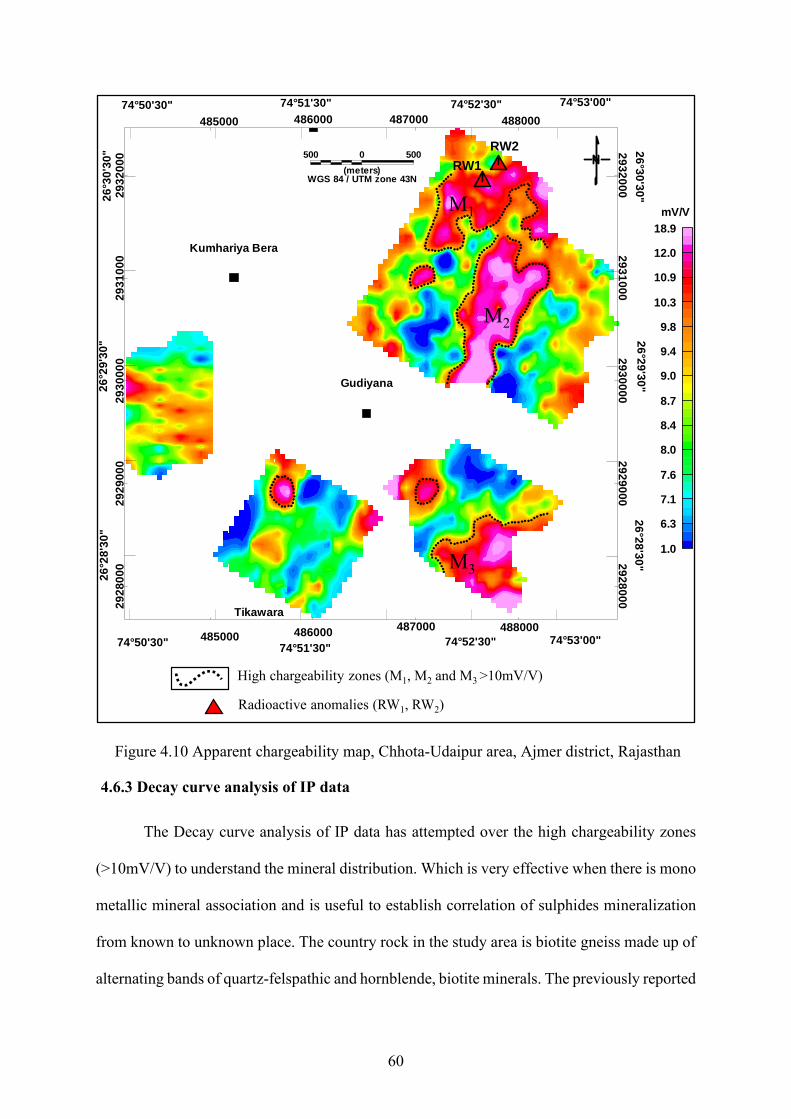
60
Figure 4.10 Apparent chargeability map, Chhota-Udaipur area, Ajmer district, Rajasthan
4.6.3 Decay curve analysis of IP data
The Decay curve analysis of IP data has attempted over the high chargeability zones
(>10mV/V) to understand the mineral distribution. Which is very effective when there is mono
metallic mineral association and is useful to establish correlation of sulphides mineralization
from known to unknown place. The country rock in the study area is biotite gneiss made up of
alternating bands of quartz-felspathic and hornblende, biotite minerals. The previously reported
High chargeability zones (M1, M2 and M3 >10mV/V)
500 0 500
(meters)WGS 84 / UTM zone 43N
1.0
18.9
6.3
7.1
7.6
8.0
8.4
8.7
9.0
9.4
9.8
10.3
10.9
12.0
mV/V
29
28
00
02
92
90
00
29
30
00
02
93
10
00
29
32
00
0
29
28
00
02
92
90
00
29
30
00
02
93
10
00
29
32
00
0
485000 486000487000 488000
485000 486000 487000 488000
26
°28
'30
"2
6°2
9'3
0"
26
°30
'30
"
26
°28
'30
"2
6°2
9'3
0"
26
°30
'30
"
74°50'30" 74°51'30" 74°52'30" 74°53'00"
74°50'30"74°51'30"
74°52'30" 74°53'00"
RW1
RW2
KMB1
Chhota Udaipur
Kumhariya Bera
Gudiyana
Tikawara
M2
M3
M1
Radioactive anomalies (RW1, RW2)

61
radioactive anomalies from Chhota Udaipur area has polymetallic character of uraninite,
molybdenite, chalcopyrite, pyrite, magnetite, ilmenite and xenotime (Sinha et al., 2002).
The different order of decay time constant can be associated with different grain size
and mineralization. As we can see in the Figure 4.11 there are two different orders of decay
constant obtained by fitting the sum of two exponential series to the observed IP decay curve
with a chi. square error of 0.10 at data point near radioactive anomaly (Rw1). The decay
constants obtained are 278 ms and 2077 ms. The first decay time constant 278 ms may
represents the sulphide mineralization and the second decay time constant 2077 ms could be
indicative of association of ferruginous material/ magnetite in gneiss. Similarly, for the IP data
point near second radioactive anomaly (RW2) the decay time constant τ1 and τ2 are 175 ms
and 1562 ms are obtained respectively, which represents less volume percentage of sulphides
and magnetite mineralisation association than compared to the RW1. The decay curve analysis
has been attempted for IP data points of 18 traverses of the high chargeability zone (>10
mV/V). The chargeability constants (a, b) and decay time constants (τ1, τ2) are estimated and
bivariate plots are generated for ‘a’ against ‘τ1’ and ‘b’ against ‘τ2’ as shown in the Figure
4.13 & 4.14 respectively.
The horizontal trend of the bivariate plot (Figure 4.13) of chargeability constant(a)
against decay time constant(τ1) signifies that the decay time constant values are varying over
narrow range of chargeability. The horizontal trend may represent the increasing of grain size
with less variation in sulphides concentration (Pelton et al., 1978). In the case of plot of
chargeability constant(b) and decay time constant(τ2) (Figure 4.14), the trend of the points is
near to vertical, which represents large variation of chargeability constant (b) values over
limited variation in decay time constant, which implies the increase in concentration of
ferruginous material/ magnetite in gneiss with less variation in grain size.

62
Figure 4.11 Chargeability decay curve analysis of IP data station near RW1
Figure 4.12 Chargeability decay plot analysis of IP data station near RW2
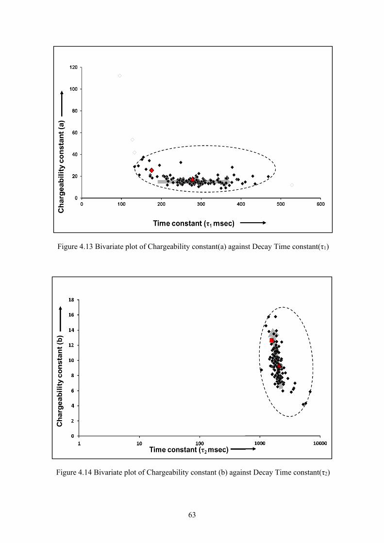
63
Figure 4.13 Bivariate plot of Chargeability constant(a) against Decay Time constant(τ1)
Figure 4.14 Bivariate plot of Chargeability constant (b) against Decay Time constant(τ2)

64
4.7 Inversion of IP/Resistivity Data
Inversion of apparent resistivity data enable to derive unambiguous interpretation of the
earth`s resistivity structure (Boonchaisuk et al., 2008). By modeling and inversion of the
IP/resistivity data true resistivity and chargeability picture of the subsurface is derived.
Inverted model depth sections have been prepared from the IP/Resistivity data along
the few traverses by using the RES2DINV program (www.geotomosoft.com). The inversion
program divides the subsurface into a number of small rectangular prisms and attempts to
determine the resistivity and chargeability values of the prisms so as to minimize the difference
between the calculated and observed apparent resistivity and chargeability values. The profile
S8E covering a total length of 1200 m, interpreted up to a depth of 240 m is shown in Figure
4.15(A).
Table 4.1 Inversion parameters of chargeability and resistivity depth section of S8E line
S. No Inversion parameters
1. Line length is 1200m
2. Electrode spacing is 50m
3. Total no. of data points are 22
4. The model has 8 layers and 102 blocks
5. Absolute error is 10.90 for resistivity data
and 1.52 for IP data
6. Average sensitivity is 0.185
The 2-D interpreted geological model section can be characterized by low to high
resistivity distributions in the range of 120-1970 Ohm.m, chargeability depth section
corresponding to the same line is shown in Figure 4.15(B). As the study area is part of the
banded gneissic complex (BGC) which contains high resistive compact metamorphic gneissic
rocks exposed on the surface, the same is reflected in the depth section. Towards south-east

65
side of the section the high resistivity distribution start from surface and increases with depth.
The progressive increase in formation resistivity indicate that the decrease in degree of
weathering of the rock units from the surface to higher depth. A prominent low resistive zone
(<179 Ohm.m) is observed in the north-west side of the section which is correlating with
moderate chargeability (>10mV/V) signature in the chargeability depth section (Figure
4.15(Q)). the low resistivity and moderate chargeability zone indicate the fractures filled with
sulphides within the BGC. The observed prominent low resistive and moderate chargeability
zone in this section is reflected from 15m to up to the depth of 80m.
Inverted depth sections have been prepared for three traverses of S6, S7 and S8 to
compare the resistivity and chargeability of three depth sections in order to know the depth as
well as strike continuity and shown in Figures 4.16 and 4.17. As shown in the table 4.2 the
following inversion parameters are utilized to prepare these inverted depth sections. In all the
three sections, it is observed that the conductive zone starts from depth of around 15m and
continues further up to 80m depth.
Table 4.2 Inversion parameters of chargeability and resistivity depth sections of S6, S7 and S8
lines
S. No Parameters description Parameters value
S6 Line S7 Line S8 Line
1. Line length 1935 1978 1978
2. Electrode spacing 50 50 50
3. Total no. of data points 42 44 44
4. No. of Model layers 12 11 11
6. No. of model blocks 807 762 762
5. Absolute error for resistivity data
and IP data
3.29
0.19
4.95
1.71
2.23
1.96
6. Average sensitivity 0.122 0.132 0.149

66
Figure 4.15 2D-Inverted depth sections (P) resistivity (Q) Chargeability of IP/Resistivity data along the traverse S8E
Inverted 2D depth sections(P- resistivity; Q-Chargeability) of IP/Resistivity data, Chhota Udaipur area, Ajmer district, Rajasthan
NW SELine no.: S8E
Low Resistivity,high chargeability zone
P
Q
Apparent Resistivity map
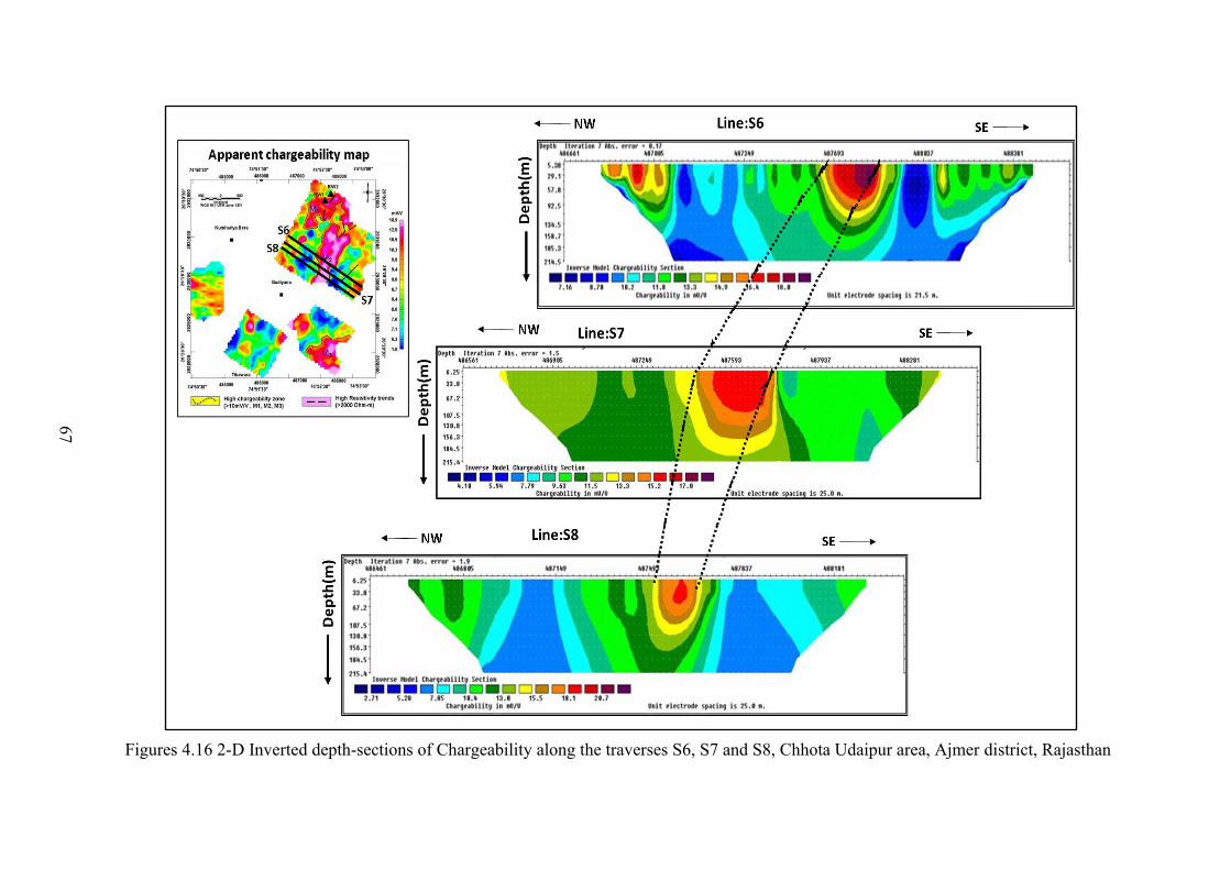
67
Figures 4.16 2-D Inverted depth-sections of Chargeability along the traverses S6, S7 and S8, Chhota Udaipur area, Ajmer district, Rajasthan
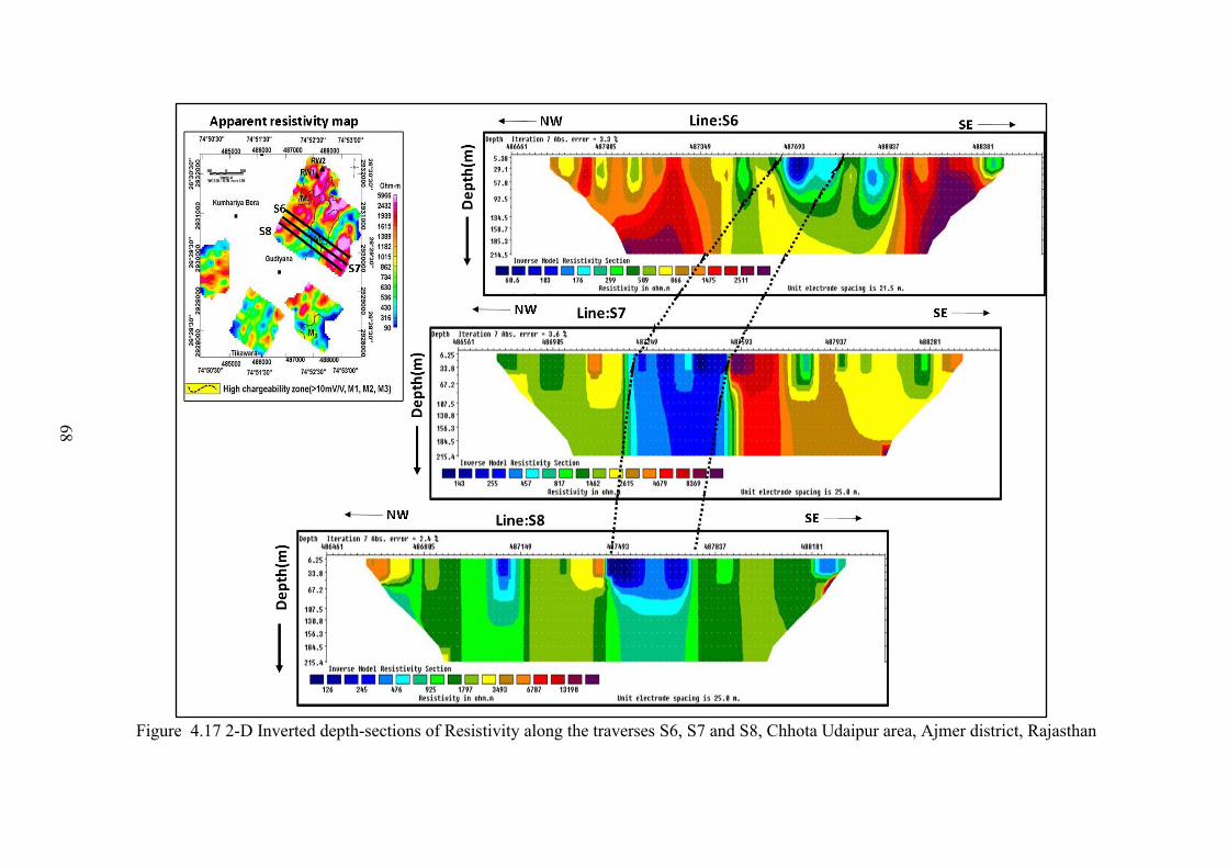
68
Figure 4.17 2-D Inverted depth-sections of Resistivity along the traverses S6, S7 and S8, Chhota Udaipur area, Ajmer district, Rajasthan

69
CHAPTER 5
INTEGRATED INTERPRETATION
The geophysical techniques are used as an indirect tool in uranium exploration. The
study and analysis of multiple physical properties and laboratory information of different rock
types in the study area along with geophysical signatures helps to resolve the ambiguities in
interpretation. Laboratory analysis has been attempted for few grab samples which are
representative of the different lithologies in the study area.
5.1 Petrographic Study
Petrographic studies of grab samples from the study area has been carried out to derive
additional information about nomenclature and mineralogy. The radioactive sample RW1
(table 3.1) in hand specimen is greyish colour, hard and compact and it contains abundant
biotite and sulphides. Under the microscope the rock is identified as hornblende biotite gneiss.
The perfect lineation is made by the alignment of hornblende and biotite as well as stretching
of quartz along the linear plane. The main ore minerals are magnetite, pyrrhotite, pyrite, and
chalcopyrite.
Figure 5.1 A1 and A2 Quartz biotite gneiss with Magnetite, Chalcopyrite and Pyrite.
Py = Pyrite, Cp = Chalcopyrite, Mt = Magnetite,

70
Mt = Magnetite, Pg = Plagioclase felspar,
Qt = Quartz, Bt = Biotite. Figure 5.2 B1 Quartz biotite gneiss with
Magnetite in transmitted light and B2)
plagioclase feldspars crystals
Figure 5.3 (C) Gneissose plane of gneiss
The thin sections of radioactive sample are shown in Figure 5.1. The sample has shown high
susceptibility of 25-570 mSI.
5.2 Hydrogeochemical study
The hydrogeochemical study provides direct information about concentration of
elements in ground water implies subsurface and often able to test the distribution of uranium
in the third dimension, giving evidence of the presence of buried deposits that may have no
surface radiometric expression. In present study, along with the magnetic and IP/Resistivity
surveys, radioactivity measurements have been made over the rock exposures using a
scintillometer. The recorded readings were in the range of 25-15 𝜇𝑅/ℎ𝑟 which are not

71
significant. Hence, water sampling has been carried out in study area to know the anomalous
radioactivity and to correlate its result with geophysical signatures.
`
Figure 5.4 Water sample locations over the RTP map of Chhota Udaipur area,
Ajmer district, Rajasthan
Total five water samples were collected from dug wells in the study area, among which
two are collected from the two radioactive wells RW1and RW2 and two are collected from the
wells falling over high magnetic, high chargeability zones and one sample is collected from a
well falling solely on alteration zones (malachite staining) (Figure 5.4). Generally, ground
500 0 500 1000
(meters)WGS 84 / UTM zone 43N
-289
1126
36
88
122
150
179
207
245
286
337
406
481
610
nT
29
28
00
02
92
90
00
29
30
00
02
93
10
00
29
32
00
02
93
30
00
29
28
00
02
92
90
00
29
30
00
02
93
10
00
29
32
00
02
93
30
00
483000 484000 485000 486000 487000 488000 489000
483000 484000 485000 486000 487000 488000 489000
26
°28
'26
°29
'26
°30
'26
°31
'
26
°28
'26
°29
'26
°30
'26
°31
'
74°50' 74°51' 74°52' 74°53'
74°50' 74°51' 74°52' 74°53'
Chhota Udaipur
Kumhariya Bera
Gudiyana
Tikawara
RW1
RW2
PW1
PSW1
KMB1
Location of Water Samples
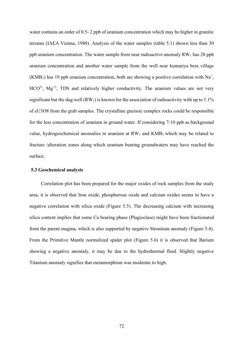
72
water contains an order of 0.5- 2 ppb of uranium concentration which may be higher in granitic
terrains (IAEA Vienna, 1988). Analysis of the water samples (table 5.1) shown less than 30
ppb uranium concentration. The water sample from near radioactive anomaly RW1 has 28 ppb
uranium concentration and another water sample from the well near kumariya bera village
(KMB1) has 19 ppb uranium concentration, both are showing a positive correlation with Na+,
HCO3-, Mg+2, TDS and relatively higher conductivity. The uranium values are not very
significant but the dug well (RW1) is known for the association of radioactivity with up to 1.1%
of eU3O8 from the grab samples. The crystalline gneissic complex rocks could be responsible
for the less concentration of uranium in ground water. If considering 7-10 ppb as background
value, hydrogeochemical anomalies in uranium at RW1 and KMB1 which may be related to
fracture /alteration zones along which uranium bearing groundwaters may have reached the
surface.
5.3 Geochemical analysis
Correlation plot has been prepared for the major oxides of rock samples from the study
area, it is observed that Iron oxide, phosphorous oxide and calcium oxides seems to have a
negative correlation with silica oxide (Figure 5.5). The decreasing calcium with increasing
silica content implies that some Ca bearing phase (Plagioclase) might have been fractionated
from the parent magma, which is also supported by negative Strontium anomaly (Figure 5.4).
From the Primitive Mantle normalized spider plot (Figure 5.6) it is observed that Barium
showing a negative anomaly, it may be due to the hydrothermal fluid. Slightly negative
Titanium anomaly signifies that metamorphism was moderate to high.
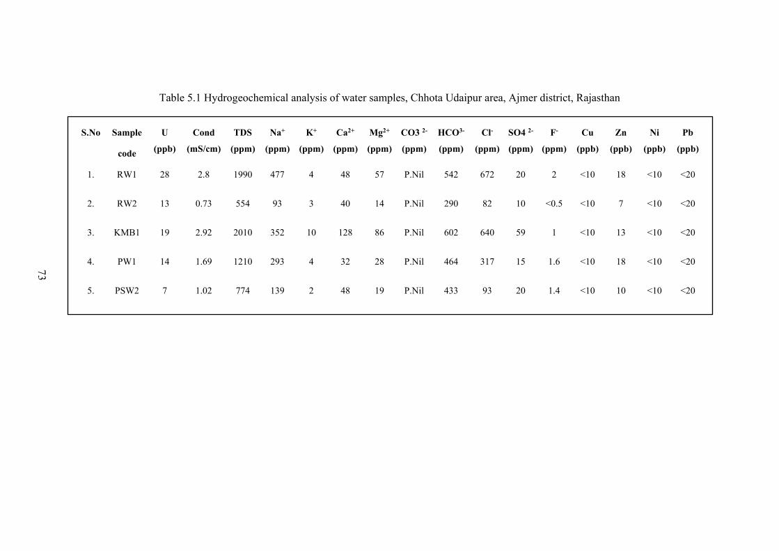
73
Table 5.1 Hydrogeochemical analysis of water samples, Chhota Udaipur area, Ajmer district, Rajasthan
S.No Sample
code
U
(ppb)
Cond
(mS/cm)
TDS
(ppm)
Na+
(ppm)
K+
(ppm)
Ca2+
(ppm)
Mg2+
(ppm)
CO3 2-
(ppm)
HCO3-
(ppm)
Cl-
(ppm)
SO4 2-
(ppm)
F-
(ppm)
Cu
(ppb)
Zn
(ppb)
Ni
(ppb)
Pb
(ppb)
1. RW1 28 2.8 1990 477 4 48 57 P.Nil 542 672 20 2 <10 18 <10 <20
2. RW2 13 0.73 554 93 3 40 14 P.Nil 290 82 10 <0.5 <10 7 <10 <20
3. KMB1 19 2.92 2010 352 10 128 86 P.Nil 602 640 59 1 <10 13 <10 <20
4. PW1 14 1.69 1210 293 4 32 28 P.Nil 464 317 15 1.6 <10 18 <10 <20
5. PSW2 7 1.02 774 139 2 48 19 P.Nil 433 93 20 1.4 <10 10 <10 <20

74
Figure 5.5 Correlation of major oxides
Figure 5.6 Primitive Mantle normalized spider plot
SiO2
SiO2
Fe2O3
Fe2O3
CaO
CaO
Al2O3
Al2O3
P2O5
P2O5
-0.97
-0.82
0.15
-0.82
0.71
-0.29
0.73
-0.06
0.90 0.01
Sample Size 9
null
very weak
weak
moderate
strong
very strong
(significance 0.90)Colour Coding

75
5.4 Profile analysis of Magnetic and IP/Resistivity data
In the image map preparation of the data, the interpolation of data by gridding
techniques sometimes may create artifacts and mask the genuine anomalies. Profile analysis
has been done for the better understanding of geophysical signatures at the two radioactive
anomalies. Profiles are taken along the two radioactive anomaly locations in NW-SE direction
perpendicular to the general trend of the geological features in the study area. Figure 5.7 shows
the location of profiles over reduced to pole magnetic map and apparent chargeability map. As
shown in Figure 5.8 the radioactive anomaly RW1 is falling in the moderate low resistivity
(~1460 Ohm.m), high magnetic (~460 nT) and moderate chargeability of 12 mV/V zone. The
second radioactive anomaly RW2 is falling in the high magnetic (~440 nT) and along gradient
of the resistivity (1520 Ohm.m) and chargeability (8.5 mV/V) zone as shown in Figure 5.9.
Figure 5.7 Profiles over RTP and Apparent chargeability maps
500 0 500 1000
(meters)WGS 84 / UTM zone 43N
-289
1126
36
88
122
150
179
207
245
286
337
406
481
610
nT
29
28
00
02
92
90
00
29
30
00
02
93
10
00
29
32
00
02
93
30
00
29
28
00
02
92
90
00
29
30
00
02
93
10
00
29
32
00
02
93
30
00
483000 484000 485000 486000 487000 488000 489000
483000 484000 485000 486000 487000 488000 489000
26
°28
'26
°29
'26
°30
'26
°31
'
26
°28
'26
°29
'26
°30
'26
°31
'
74°50' 74°51' 74°52' 74°53'
74°50' 74°51' 74°52' 74°53'
Chhota Udaipur
Kumhariya Bera
Gudiyana
Tikawara
RW1
RW2
High chargeability zones (M1, M2 and M3 >10mV/V)
500 0 500
(meters)WGS 84 / UTM zone 43N
1.0
18.9
6.3
7.1
7.6
8.0
8.4
8.7
9.0
9.4
9.8
10.3
10.9
12.0
mV/V
29
28
00
02
92
90
00
29
30
00
02
93
10
00
29
32
00
0
29
28
00
02
92
90
00
29
30
00
02
93
10
00
29
32
00
0
485000 486000487000 488000
485000 486000 487000 488000
26
°28
'30
"2
6°2
9'3
0"
26
°30
'30
"
26
°28
'30
"2
6°2
9'3
0"
26
°30
'30
"
74°50'30" 74°51'30" 74°52'30" 74°53'00"
74°50'30"74°51'30"
74°52'30" 74°53'00"
RW1
RW2
KMB1
Chhota Udaipur
Kumhariya Bera
Gudiyana
Tikawara
M2
M3
M1
Radioactive anomalies (RW1, RW2)
Profiles over RTP and Apparent Chargeability maps
A
A1
B
B1
A
A1
B
B1
A
A1Profile along radioactive anomaly RW1
B
B1
Profile along radioactive anomaly RW2

76
Figure 5.8 Profile analysis of magnetic and IP/Resistivity data along RW1 line
0.0
2.0
4.0
6.0
8.0
10.0
12.0
14.0 S600EN600W
Radioactive anomaly (RW1) Uranium concentration in water sample -28 ppb
0
100
200
300
400
500
600
0
500
1000
1500
2000
2500
3000
3500
4000
4500
5000
487200 487400 487600 487800 488000 488200
Fracture zone
AA1
Apparent Chargeability (mV/V)
Apparent Resistivity (Ohm-m)
Magnetic-RTP (nT)
Ohm.mmV/V nT

77
Figure 5.9 Profile analysis of magnetic and IP/Resistivity data along RW2 line
0.0
2.0
4.0
6.0
8.0
10.0
12.0
14.0
16.0
0
100
200
300
400
500
600
0
500
1000
1500
2000
2500
3000
3500
487300 487500 487700 487900 488100 488300
S600EN600W
Radioactive anomaly (RW2), Uranium concentration in water sample -13 ppb
B B1
Fracture zone
Apparent Chargeability (mV/V)
Apparent Resistivity (Ohm-m)
Magnetic-RTP (nT)
Ohm.mmV/V nT

78
Figure 5.10 (a) Integrated structural features and high chargeability zones over FVD of RTP map
(b) Resistivity contour map of Chhota Udaipur area, Ajmer district, Rajasthan
500 0 500
(meters)WGS 84 / UTM zone 43N
29
28
00
02
92
90
00
29
30
00
02
93
10
00
29
32
00
0
29
28
00
02
92
90
00
29
30
00
02
93
10
00
29
32
00
0
485000 486000487000 488000
485000 486000 487000 488000
26
°28
'30
"2
6°2
9'3
0"
26
°30
'30
"
26
°28
'30
"2
6°2
9'3
0"
26
°30
'30
"74°50'30" 74°51'30" 74°52'30" 74°53'00"
74°50'30"74°51'30"
74°52'30" 74°53'00"
RW1
RW2
KMB1
Chhota Udaipur
Kumhariya Bera
Gudiyana
Tikawara
b
500 0 500 1000
(meters)WGS 84 / UTM zone 43N
-2.05
2.34
-0.62
-0.44
-0.32
-0.22
-0.14
-0.05
0.03
0.11
0.20
0.29
0.41
0.59
nT/m
2928000
2929000
2930000
2931000
2932000
2933000
2928000
2929000
2930000
2931000
2932000
2933000
483000 484000 485000 486000 487000 488000 489000
483000 484000 485000 486000 487000 488000 489000
26°2
8'
26°2
9'
26°3
0'
26°3
1'
26°2
8'
26°2
9'
26°3
0'
26°3
1'
74°50' 74°51' 74°52' 74°53'
74°50' 74°51' 74°52' 74°53'
Chhota Udaipur
Kumhariya Bera
Gudiyana
Tikawara
RW1
RW2
aM1
M2
M3
M1
M2
M3
Inferred fault/fractures
Trend of the high magnetic bodies ( >400 nT)
High chargeability zones (M1, M2 and M3 >10 mV/V)
Low Resistivity Trends (<1500 Ohm.m)
Radioactive anomalies (RW1, RW2)

79
The combined analysis of chargeability, resistivity and magnetic data of the area is
shown in Figure5.10(A) and 5.10(B). By integrating of the high chargeability zone (>10 mV/V)
with first vertical derivative of RTP and resistivity contour maps indicated that the high
chargeability zones (M1, M2, M3) are coinciding with the low to moderate resistivity values
(90-1500 Ohm.m). The high chargeability zone- M1 is correlating with moderate high magnetic
values (380-440 nT) which is vindicated by the petrographic study of grab sample (Figure
5.1A1and A2) as the magnetite mineralization is present in the fractured/altered BGC is
responsible for high magnetic, while presence of Chalcopyrite and pyrite for high chargeability.
The association of similar geophysical signatures that are high magnetic, low resistivity and
high chargeability values have been observed in the south east of the study area and demarcated
as target zone.
Geochemical analysis of grab samples also revealed that the alteration and
hydrothermal activity might have been taken place and iron oxide gets precipitated along with
other minerals along the fractures. Based on the petrographic and hydrogeochemical studies,
high magnetic signatures near kumariya bera (KMB1) village is caused by ilmenite and
magnetite mineralisation in biotite gneiss which may be significant as it has anomalous anion
and cation concentrations which are comparable with that of sample from RW1.
Integrated interpretation of magnetic and IP/resistivity data including geophysical
profile analysis, laboratory analysis and physical property measurements of grab rock samples
and hydro geochemical studies, it is found that high chargeability zones (>10 mV/V) which are
well correlated with the moderate to low resistivity (< 1500 Ohm.m) and moderate high
magnetic zones (>400 nT) could be favourable locales for uranium mineralization in this area

80

81
CHAPTER 6
CONCLUSIONS
Detailed ground geophysical surveys comprising of Induced polarization/Resistivity
and Magnetic surveys were conducted in and around Chhota-Udaipur area, Ajmer district,
Rajasthan. The study area is geologically highly deformed and contains moderate to high grade
metamorphic rocks of Sandamata complex of Archean age, which has been subjected to
hydrothermal alteration as revealed by the laboratory studies of grab samples and supported by
the field observations.
Magnetic data over 30 sq. km area facilitated in demarcating faults/fractures trending
in E-W, NE-SW and NW-SE directions. Three prominent high magnetic anomalies have been
recorded and interpreted in terms of mafic intrusive bodies/magnetite mineralization in banded
gneissic complex. 2-D and 3-D modeling of magnetic data enabled in deciphering the location
and geometry of the structures in the study area. The derived plausible geological models
provided useful information for further planning of sub surface exploration program.
From IP/Resistivity surveys, three high chargeability zones (M1, M2 and M3) have been
successfully delineated. The NE-SW trending zone-M1 has strike length of around 600 m with
width of 90 to 130 m and continues further north-east. The radioactive anomalies are located
in this high chargeability zone and associated with the geophysical signatures of moderately
low resistivity (1460 Ohm.m) and high magnetic (460 nT). The second zone-M2 in the eastern
side of the study area has strike length of 1.5 km with width of 300 to 350 m and third zone-
M3 in the south east of the study area. The high chargeability zones are correlating with low
resistivity and interpreted as the fracture/alteration zones filled with disseminated sulphides in
BGC. Inverted depth sections of high chargeability zones yielded necessary information
regarding the size, depth and width of the conductive body in the sub surface.

82
Based on integrated interpretation of geophysical data including profile analysis, laboratory
analysis and physical property measurements of grab rock samples and hydro geochemical
studies it is inferred that high chargeability zones (>10 mV/V) associated with the moderate to
low resistivity (< 1500 Ohm.m) and moderate high magnetic zones (>400 nT) represents
alteration zones which could be favourable locales for uranium mineralization in the area
The present study has brought out the structural features and favourable target zones
for uranium mineralisation in the study area by employing Magnetic and IP/Resistivity
techniques. Future work includes after drilling of these anomalous zone, geophysical
multiparameter logging has to be carry out to record the physical properties of formations against
depth, which directly provides the subsurface information. The integration of surface and borehole
database will provide detail understanding and genesis of the geology of the area and also this results will
be used for precise subsurface modeling which also facilitate in adapting new techniques to define the
subsurface structures and ore body with improved accuracy.
.

83
PUBLICATION TITLE: “Application of Magnetic and IP/Resistivity methods to Delineate the Structural Features
and conductive zones: A case study from Chhota-Udaipur area, Ajmer district,
Rajasthan”
*The above titled paper would be prepared for publication

84

85
REFERENCES
Austin, Jim., Andreas Björk., Ben Patterson., (2019). Structural controls of the Ernest Henry
IOCG deposit: Insights from integrated structural, geophysical and mineralogical
analyses. AEGC, From Data to Discovery – Perth, Australia.
Baranov, V., Naudy, H., (1964). Numerical calculation of the formula of reduction to the
magnetic pole. Geophysics. vol. 29, pp. 67-79.
Boonchaisuk, S., Vachiratienchai, C., and Siripunvaraporn, W., (2008). Two Dimensional
direct current (DC) resistivity inversion: Data space Occam`s approach: Physics of the
Earth and Planetary Interiors, vol. 168, p. 204-211.
Borner, F.D., Schopper, W. and Weller, A., (1996), Evaluation of transport and storage
properties in the soils and groundwater zone from induced polarization measurements,
Geophysical Prospecting, vol. 44(4), pp. 583-601.
Briggs, I.C., (1974). Machine contouring using minimum curvature. Geophysics, vol. 39, pp.
39-48.
Clark, D, A., French, D. H., Lackie, M. A., and Schmidt, P. W., (1992). Magnetic petrology:
Application of integrated rock magnetic and petrological techniques to geological
interpretation of magnetic suveys. Exploration geophysics, vol. 23, pp. 65-68.
Crawford, A.R., (1970). The Precambrian geochronology of Rajasthan and Bundelkhand,
northern India, Can. J. Earth Sci. vol. 7, pp. 91–110.
Cull, J.P. & Massie, D., (2002). Aquifer mapping and groundwater quality in faults and
fractures. Exploration Geophysics, vol. 33(2), pp. 122-126.
Dash, J. K., S. Sethuram, V. Ramesh Babu and M. N. Chary, (2006). Target delineation for
uranium exploration in the southern margin of Bhima basin – A Geophysical case study,
86
Third International seminar and exhibition on exploration geophysics: Journal of
Geophysics, AEG, pp. A18.
Dentith, M., Mudge, S.T., (2014). Geophysics for the mineral exploration Geoscientist,
Cambridge University press.
Dhirenda Kumar Pandey., Alfred Uchman., Vineet Kumar., Rajesh Singh Shekhawat., (2014).
Cambrian trace fossils of the Cruziana ichnofacies from the Bikaner-Nagaur Basin, north
western Indian Craton. Journal of Asian Earth Sciences, Vol. 81, pp. 129–141.
Dobrin, M.B., Savit, C.H., (1988). Introduction to Geophysical Prospecting. Fourth edition,
McGraw-Hill, New York. p. 882.
Esdale Donald., Pridmore, Don F., Coggon, John., Philip Muir, Peter Williams., Frank Fritz.,
(2003). The Olympic Dam copper-uranium-gold-silver-rare earth element deposit, South
Australia: A geophysical case history, ASEG Extended Abstracts, pp. 147-168.
GEM System., (2008). GSM-19 v7.0 Instruction manual. Manual release 7.4, GEM Systems,
Canada.
Gupta, S. N., Arora, Y. K., Mathur, R. K., Iqbaluddin, Parsad, B., Sahai, T. N., and Sharma, S.
B., (1997). The Precambrian geology of the Aravalli region, Southern Rajasthan and
northeastern Gujarat, Geological Survey of India, pp. 123.
Henkel, H., Guzman, M., (1977). Magnetic features of fracture zones. Geoexploration, vol.
15(3), pp. 173-181.
Heron, A.M., (1953). The Geology of central rajaputhana. Geological society of India, vol. 79,
p.389
87
Hong-Rui Fan., Kui-Feng Yang., Fang-Fang Hu., Shang Liu., Kai-Yi Wang., (2016). The giant
Bayan Obo REE-Nb-Fe deposit, China: Controversy and ore genesis. Geoscience
Frontiers vol.7, pp. 335-344.
International Atomic Energy Agency, Vienna, (1988). Geochemical Exploration for Uranium,
technical reports series no. 284.
Kamlesh Kumar., (2018). Uranium mineralization in the Khetri sub-basin, North Delhi fold
belt, India. poster, URAM-2018.
Kearey, P., Brooks, N., Hill, I., (2002). An Introduction to Geophysical Exploration. 3rd edition,
Blackwell Science. p. 281.
Khandelwal, M.K., Bisht, B.S., Tiwary, A., Dash, S.K., Mundra, K.L., Padhi ,Ajoy.K., Nanda,
L.K. and Maithani, P.B., (2008). Uranium-copper–molybdenum association in the Rohil
Deposit, North Delhi Fold Belt, Rajasthan. Mem. Geological society of India, vol. 73,
pp. 117-130.
Loke, M. H., (2016).Tutorial: 2-D and 3-D electrical imaging surveys, pp. 207.
Loke, M. H., (2011). Electrical resistivity surveys and data interpretation. In Encyclopedia of
Solid Earth Geophysics, Springer, Dordrecht. pp. 276-283.
Loke, M.H., (2000). Electrical imaging surveys for environmental and engineering studies: A
practical guide to 2-D and 3-D surveys, p. 61
Lopez-Loera, H., U.-Fucugauchi, J., A-Valdivia, L.M., (2010). Magnetic characteristics of
fracture zones and constraints on the subsurface structure of the Colima Volcanic
Complex, Western Mexico. Geosphere, vol. 6 (1), pp. 35–46.
Lowrie, W., (2007). Fundamentals of Geophysics, Second edition: Cambridge University
Press, New York. p. 393.
88
Marshall, J.D., and Madden, T.R., (1959). Induced, polarization, a study of its causes,
Geophysics, Vol. 24, pp. 790-816.
Miller, H. G., and Singh, V., (1994). Potential field tilt: A new concept for location of potential
field sources. Journal of Applied Geophysics, vol. 32, pp. 213–217.
Mishra, B., Kumar, K., Khandelwal, M.K., and Nanda, L.K., Uranium mineralization in the
Khetri sub-basin, North Delhi fold belt, India. Geological Society of India, pp 285 to 288.
Nabighian, M.N., Grauch, V.J.S., Hansen, R.O., LaFehr, T.R., Li, Y., Peirce, J.W., Phillips,
J.D. & Ruder, M.E., (2005). The historical development of the magnetic method in
exploration. Geophysics, vol. 70 (6), pp. 33-61.
Paterson, N.R., Reeves, C.V., (1985). Applications of gravity and magnetic surveys: the state
of the-art in 1985. Geophysics, vol. 50, pp. 2558–94.
Pedersen, L. B., (1979). Constrained inversion of potential field data: Geophysical Prospecting,
Vol. 27, pp. 726–748.
Pelton, W.H., Ward, S.H., Hallof, P.G., Sill, W.R., and Nelson, P.H., (1978). Mineral
discrimination and removal of inductive coupling with multi-frequency IP, Geophysics,
Vol. 43, pp. 588-609.
Peters, L.J., (1949). The direct approach to magnetic interpretation and its practical application.
Geophysics, vol. 14, pp. 290–320.
Powell, B., Wood, G., Bzdel, L., (2007), Advances in Geophysical Exploration for Uranium
Deposits in the Athabasca Basin, Proceedings of Exploration 07, pp. 771-790
Radhakrishna murthy, I.V., and Rama Rao, B.S., (1978). Gravity and Magnetic methods of
prospecting. Gulab vazirani publishers -India, p. 390.
Ramakrishnan, M., Vaidyanathan, R., (2010). Geology of India. Geological society of India.

89
Ramesh Babu, V., 2007. Modeling and Inversion of Magnetic and VLF-EM data for Uranium
Exploration, Raigarh district, Chhattisgarh, India: PhD Thesis, Osmania University.
Reid, A. B., J. M. Allsop, H. Granser, A. J. Millett, and I. W. Somerton, (1990). Magnetic
interpretation in three dimensions using Euler deconvolution: Geophysics, vol. 55, pp.
80–91
Roberts, C.L., Smith, S.G., (1994). A new magnetic survey of Lundy Island, Bristol Channel.
Proceedings of the Ussher Society, vol. 8 (3), pp. 293-297.
Salem Ahmed., Simon Williams , Derek Fairhead, Richard Smith, and Dhananjay Ravat,
(2008). Interpretation of magnetic data using tilt-angle derivatives. Geophysics, Vol. 73,
pp. L1–L10.
Satyanarayana, K. V., Mahender, S., and Rama Rao, J. V., (2018). Multi parameter
geophysical Surveys for Identification of Geological Environment favorable for base
metal mineralization in mallapuram block, Markapur base metal Belt, Cuddapah Basin.
Jour. of Geophysics, Vol. XXXIX No.2, pp 51-56.
Satyanarayana, M. V., Subhash Ram., Navin Goyal, Srinivasan, S., Srinivas, R., Nanda, L.
K., and Chaturvedi, A. K., (2014). Delineation of Structure over Karara-Tavidar
Volcanics of Jalore District, Rajasthan, by Magnetic and Gravity Investigations - An
Appraisal of the Integrated Results. Jour. of Geophysics. XXXV No.4, pp 159-165.
Seigel, H.O., (1959). Mathematical formulation and type curves for induced polarization,
Geophysics, Vol. 24, No. 3,pp. 547-565.
Seigel, H.O., Vanhala, H., and Sheard, S.N., (1997). Some case histories of source discrimination
using time-domain spectral IP, Geophysics, Vol. 62, No. 5, pp. 1394- 1408.
Shrajala Pitla., SrinivasaRao, B., Allipeera, P., Subhash Ram., Chaturvedi, A.K., (2015).
Application of geophysical techniques in uranium exploration along the albitite line,
90
Kerpura-Karoi area, Sikar district, Rajasthan. Jour. of Geophysics, Vol. XXXVI No.2,
pp 95-102.
Sinha, D. K., SohailFahmi, Sarkar, B.C., and Roy, M.K., (2002). Discovery of the uraniferous
polymetallic veins in the gneisses of Chhota-Udaipur, Ajmer District, Rajasthan.
Geological Society of India, Vol.59, pp. 469 - 472.
Sinha-Roy, S., Malhotra, G., Mohanty, M., (1998). Geology of Rajasthan. Geological Society
of India. p.278
Spector, A., Grant, F.S., (1970). Statistical models for interpreting aeromagnetic data:
Geophysics, vol. 35. pp. 293-3302.
Srinivasa Rao, S., Krishna chaithanya, K., Deepak Kumar., (2018). Annual report on detailed
induced polarization (IP) / resistivity and magnetic surveys in the west and east of Rohil
deposit, Sikar district, Rajasthan. Unpublished report, AMD/DAE.
Srinivasa Rao, B., Subashram., Shaik Roshan Ali., Viney Kumar., Dash, J. K., Purohit, R. K.,
and Chaturvedi, A. K., (2016). Application of Integrated Geophysical Techniques to
Delineate Favourable Structures and Conductive Zones for Uranium Mineralization in
Narasinghpuri-Salwari Areas, Sikar District, Rajasthan. Jour. of Geophysics, Vol.
XXXVII No.4, pp. 191-196
Subash Ram., Nepal Singh., Kumar, B.V.L., Srinivas, R., (1999). Brief annual report on detailed
geophysical surveys at Chhota Udaipur area, Ajmer district , Rajasthan.. Unpublished report,
AMD/DAE.
Sumner, J.S., (1976). Principles of induced polarization for geophysical exploration: Elsevier
Science Publ. Co., Inc. p. 276

91
Sumit Kumar Ray., (1987). Albitite occurrences and associated Ore Minerals in the Khetri
Copper belt, North-Eastern Rajasthan. Geological Society of India, Vol. 113-7, pp.41-
49.
Telford, W.M., Geldart, L.P., and Sheriff, R.E., (1990). Applied Geophysics, Cambridge
University Press, 2nd edition, pp. 289-291.
Thompson, D. T. (1982), A new technique for making computer-assisted depth estimates
from magnetic data: Geophysics, vol.47, pp.31–37.
Tuncer Volkan , Martyn J. Unsworth1 , Weerachai Siripunvaraporn , and James A. Craven.,
(2006). Exploration for unconformity-type uranium deposits with audiomagnetotelluric
data: A case study from the McArthur River mine, Saskatchewan, Canada, Geophysics,
vol. 71, pp. 201–209.
Vijaya Kumar, V., Shrajala Pitla., Siva Krishna, Y., Shashank Shekar Mishra., (2015). Annual
report on regional magnetic and detailed ip/resistivity surveys in mawata-jahaz-bera ki
dhani block, Jhunjhunu district, Rajasthan. Unpublished report, AMD/DAE.
https://www.agiusa.com/blog/comparison-11-classical-electrode-arrays
https://www.eoas.ubc.ca
http://www.gemsys.ca/versatile-proton-magnetometer
http://www.geosoft.com
http://www.iris-instruments.com
http://www.tensor-research.com.au
https://www.yumpu.com/user/terraplus.ca
https://www.world-nuclear.org