modeling and performance analysis of public safety

MODELING AND PERFORMANCE ANALYSIS OF PUBLIC SAFETY WIRELESS NETWORKS

Jiaqing Song B .Eng . , Soochow University, China, 2000

THESIS SUBMITTED IN PARTIAL FULFILLMENT OF THE REQUIREMENTS FOR THE DEGREE OF

MASTER OF APPLIED SCIENCE

In the School

of Computing Science

O Jiaqing Song 2005

SIMON FRASER UNIVERSITY

Spring 2005

All rights reserved. This work may not be reproduced in whole or in part, by photocopy

or other means, without permission of the author.

APPROVAL

Name:

Degree:

Title of Thesis:

Jiaqing Song

Master of Applied Science

Modeling and Performance Analysis of Public Safety Wireless Networks

Examining Committee:

Chair: Dr. Jian Pei Assistant Professor of School of Computing Science

Date Defended:

Dr. Ljiljana Trajkovit Senior Supervisor Professor of School of Engineering Science

Dr. Qianping Gu Supervisor Professor of School of Computing Science

Dr. Uwe Glasser Internal Examiner Associate Professor of School of Computing Science

January 26,2005

SIMON FRASER UNIVERSITY

PARTIAL COPYRIGHT LICENCE

The author, whose copyright is declared on the title page of this work, has granted to Simon Fraser University the right to lend this thesis, project or extended essay to users of the Simon Fraser University Library, and to make partial or single copies only for such users or in response to a request from the library of any other university, or other educational institution, on its own behalf or for one of its users.

The author has further granted permission to Simon Fraser University to keep or make a digital copy for use in its circulating collection.

The author has further agreed that permission for multiple copying of this work for scholarly purposes may be granted by either the author or the Dean of Graduate Studies.

It is understood that copying or publication of this work for financial gain shall not be allowed without the author's written permission.\

Permission for public performance, or limited permission for private scholarly use, of any multimedia materials forming part of this work, may have been granted by the author. This information may be found on the separately catalogued multimedia material and in the signed Partial Copyright Licence.

The original Partial Copyright Licence attesting to these terms, and signed by this author, may be found in the original bound copy of this work, retained in the Simon Fraser University Archive.

W. A. C. Bennett Library Simon Fraser University

Burnaby, BC, Canada

ABSTRACT

Public safety wireless networks (PSWNs) play a vital role in operations of

emergency agencies such as police and fire departments. In this thesis, we describe

analysis and modeling of traffic data collected from the Emergency Communications for

Southwestern British Columbia (E-Comm) PSWN.

We analyze network and agency call traffic and find that lognormal distribution

and exponential distribution are adequate for modeling call holding time and call inter-

arrival time, respectively. We also describe a newly developed wide area radio network

simulator, named WarnSim. We use WarnSim simulations to validate the proposed traffic

model, evaluate the performance of the E-Comm network, and predict network

performance in cases of traffic increase. We also provide recommendations on allocating

E-Comm network resources to deal with the increased traffic volume.

DEDICATION

To my father Kejun Jia, my mother Shen'an Song, and my wife Zhen Yuan.

ACKNOWLEDGMENTS

There are few things in the world that a person could accomplish alone. Writing

this thesis is certainly not one of them. I would like to express my special thanks to my

senior supervisor Dr. Ljiljana TrajkoviC for the continuously guidance and everlasting

support she has been giving me throughout my graduate studies.

My sincere gratitude goes to Dr. Qianping Gu, for being my supervisor and being

my advising voice on my thesis. Furthermore, I would like to express appreciation to Dr.

Uwe Glasser and Dr. Jian Pei for being on my examining committee and for giving me

valuable suggestions on my thesis.

Finally, I would like to thank all members of the Communication Networks

Laboratory at Simon Fraser University for numerous and enlightening discussions.

TABLE OF CONTENTS

.. Approval ............................................................................................................................ 11

... Abstract ............................................................................................................................. 111

......................................................................................................................... Dedication iv

Acknowledgments .............................................................................................................. v

Table of Contents ............................................................................................................. vi ...

List of Figures ................................................................................................................. vm

List of Tables .................................................................................................................... ix

Glossary ............................................................................................................................ xi

.................................................................................................... Chapter 1: Introduction 1 ....................................................................................................... 1.1 Motivation 1 ........................................................................................................ 1.2 Objectives 2

...................................................................................... 1.3 Organization of thesis 2

Chapter 2: Background ..................................................................................................... 3 .................................................................................. 2.1 Introduction to E-Comm 3

..................................................................................... 2.1.1 History of E-Comm 3 2.1.2 E-Comm network architecture ..................................................................... 4 2.1.3 Simulcast system ......................................................................................... 5 2.1.4 Transmission trunking and message trunking ............................................. 5 2.1.5 Push-to-talk mechanism ............................................................................... 6

.......................................................................... 2.1.6 Talk group and group calls 6 .......................................... 2.1.7 Systems and channels of the E-Comm network 7

............................................... 2.1.8 Mobility of radio devices and call handover 7 2.2 A sample of the E-Comm traffic data .............................................................. 8

Chapter 3: Traffic data analysis ..................................................................................... 11 3.1 Traffic data pre-processing ............................................................................ 11

............................................................................ 3.2 Traffic data characteristics 13 ............................................................. 3.2.1 Hourly and daily call arrival rates 13

....................................................................................... 3.2.2 Call holding time 17 ................................................................... 3.2.3 Agencies and call arrival rates 18

3.2.4 Systems and call arrival rates .................................................................... 19 3.3 Busy hours ..................................................................................................... 20

Chapter 4: Statistical traffic modeling ........................................................................... 22 ...................................................................... 4.1 Modeling/simulation approach 22

...................................................... Introduction to traditional traffic models 23 ............................................................................................ Erlang models 23

........................................................................... Failure of Erlang models 25 .................................................................. Traffic modeling on agency level 25

........................................................................... Modeling call holding time 27 ................................................................ Maximum likelihood estimation 27

................................................ Kolmogorov-Smirnov goodness-of-fit test 28 ........................................ Survey of existing models for call holding time 29

............................................................... Model comparison and selection 30 Modeling call inter-arrival time ..................................................................... 33

................................. Survey of existing models for call inter-arrival time 33 Model comparison and selection ............................................................... 34

..................................................................................... Call coverage pattern 36

.............................................................. Chapter 5: WarnSim: a Simulator for PSWN 37 ....................................................................................................... 5.1 Overview 37

........................................................................... 5.2 Modules and call flowchart 38 ............................................................................. 5.3 WarnSim simulation steps 43

......................................................................................... 5.4 WarnSim interface 44 ................................................................. 5.5 Validation of WarnSim simulator 49

..................................................... 5.6 Scalability and performance of WarnSim 50

........................................................................... Chapter 6: Simulation and prediction 51 ....................................................... 6.1 Validation of the proposed traffic model 51

.............................................. 6.2 Evaluation of E-Comm network performance 52 ................................................. 6.2.1 Network performance during busy hours -52 ................................................ 6.2.2 Number of channels and Grade of Service 55

.......................................... 6.2.3 Maximum queuing time and Grade of Service 57 ......................................... 6.3 Prediction of the E-Comm network performance 59

............................................................................. 6.3.1 Simulation scenario one 59 6.3.2 Simulation scenario two ............................................................................ 61

...................................................................... Chapter 7: Conclusions and future work 63

...................................................................... 7.1 Conclusions and contributions 63 ................................................................................................... 7.2 Future work 64

........................................ Appendix A: Maximum likelihood estimation (mle) scripts 65

......................................................................................................................... References 67

vii

LIST OF FIGURES

Figure 2.1. System architecture of EDACS ......................................................................... 4 Figure 3.1. Plot of the hourly call arrival rate over 30 days in year 2002 ......................... 13

Figure 3.2. Plot of the hourly call arrival rate over 92 days in year 2003 ......................... 14 Figure 3.3: Power spectrum of hourly call amval from the 2003 dataset indicates

a strong daily cyclic pattern ......................................................................... 15 Figure 3.4: Power spectrum of daily call arrival from the 2003 dataset indicates a

strong weekly cyclic pattern ......................................................................... 15 Figure 3.5. Average hourly call amval rate over 24 hours ................................................ 16

Figure 3.6. Average daily call arrival rate over seven days ............................................... 17 Figure 3.7. Hourly average of call holding time over 92 days in year 2003 ..................... 17

Figure 3.8: Power spectrum of average hourly call holding time indicates a weekly cyclic pattern .................................................................................... 18

Figure 5.1: WarnSim: (a) module hierarchical diagram and (b) relationship diagram ........................................................................................................ -38

Figure 5.2. High level diagram of the WarnSim simulator ............................................... 41 Figure 5.3: Pseudo-code corresponding to the high level diagram of the WarnSim

simulator ...................................................................................................... -42 Figure 5.4. WarnSim: (a) network topology and (b) network configuration screen ......... 45 Figure 5.5. WarnSim traffic source configuration screen: importing traffic ..................... 46

Figure 5.6. WarnSim traffic source configuration screen: generating traffic .................... 46 Figure 5.7: WarnSim simulation results screens for channel utilization of

Vancouver system during: (a) a sample week in 2002 and (b) a sample week in 2003 . The graphs show the running average calculated over ten-minute intervals ............................................................ 47

Figure 5.8: WamSim simulation results screens for the cumulative number of blocked calls in Vancouver system during: (a) a sample week in 2002 and (b) a sample week in 2003 ............................................................ 48

Figure 6.1 : Relationship between number of channels, call bloclung probability, and channel utilization . Maximum queuing time is set to zero .................... 57

Figure 6.2. Maximum call queuing time vs . call blocking probability .............................. 59

LIST OF TABLES

Table 2.1: Number of channels deployed in each E-Comm system as of December ................................................................................................................ 2003 7

................... Table 2.2. A sample of raw traffic data collected from the E-Comm network 9

Table 2.3. Descriptions of data fields in the E-Comm traffic data table ........................... 10 Table 3.1 : A sample of the processed call traffic data ....................................................... 12

................................................... Table 3.2. Agencies and average daily call arrival rates 19

..................................................... Table 3.3. Systems and average daily call arrival rates 20

Table 3.4. The top three busiest hours in 2002 and 2003 traffic datasets .......................... 21 Table 4.1: Aggregated number of calls during the top three busiest hours in 2002

....................................................................................................... and 2003 26

................................................. Table 4.2. Regrouped agencies and the original agencies 26 ................................................... Table 4.3. Candidate distributions for call holding time 31

Table 4.4: Test of candidate distributions for call holding time of Agency A during busy hours in the 2002 dataset .......................................................... 32

Table 4.5: Test of candidate distributions for call holding time of Agency B during the top three busy hours in the 2002 dataset ..................................... 32

Table 4.6: Test of candidate distributions for call holding time of Agency C during the top three busy hours in the 2002 dataset ..................................... 33

............................................ Table 4.7. Candidate distributions for call inter-arrival time 34

Table 4.8: Test of candidate distributions for call inter-arrival time of Agency A during the top three busy hours in the 2002 dataset ..................................... 35

Table 4.9: Test of candidate distributions for call inter-arrival time of Agency B during the top three busy hours in the 2002 dataset ..................................... 35

Table 4.10: Test of candidate distributions for call inter-arrival time of Agency C during the top three busy hours in the 2002 dataset ..................................... 36

Table 4.11: A sample of call coverage pattern of Agency A during the top three busy hours in 2003 ....................................................................................... 36

Table 5.1: Comparison of call blocking probability predicted by Erlang B model ................................. and the WarnSim simulated call blocking probability 49

Table 6.1. Distribution parameters for the WarnSim call generator .................................. 51

Table 6.2. System IDS and number of channels ................................................................ 51 Table 6.3: Comparison of network performance: using collected traffic (actual)

vs . model generated traffic (simulated) ........................................................ 52

Table 6.4: System IDS and number of channels during the top three busy hours in the 2003 dataset ............................................................................................ 53

Table 6.5. Simulation results of the busiest hour in the 2003 dataset ................................ 54 Table 6.6. Simulation results of the second busiest hour in the 2003 dataset ................... 54

Table 6.7. Simulation results of the third busiest hour in 2003 dataset ............................. 55 Table 6.8: Relationship between number of channels. call blocking probability,

and channel utilization . Maximum queuing time is set to zero .................... 56 Table 6.9. Maximum call queuing time vs . call blocking probability ............................... 58

.............................................................. Table 6.10. System IDS and number of channels 59 Table 6.1 1: Scenario one: distribution parameters for the WarnSim call generator .......... 60 Table 6.12: Comparison of network performance . Scenario one: using collected

traffic (original) vs . model generated traffic after the increase (predicted) . Cells with call blocking probability higher than 3% are marked in grey .............................................................................................. 60

Table 6.13. Scenario two: distribution parameters for the WarnSim call generator ......... 61 Table 6.14: Comparison of network performance . Scenario two: using collected

traffic (original) vs . model generated traffic after the increase (predicted) . Cells with call blocking probability higher than 3% are marked in grey .............................................................................................. 62

GLOSSARY

CDF Cumulative Density Function

E-Comm Emergency Communications for Southwestern British Columbia Inc.

ECDF Empirical Distribution Function

EDACS Enhanced Digital Access Communications System

FIFO First In First Out

GoS Grade of Service

GVRD Great Vancouver Regional District

K-S GoF test Kolmogorov-Smirnov Goodness-of-Fit Test

LMR Land Mobile Radio

MLE Maximum Likelihood Estimation

PDF Probability Density Function

PAMR Public Access Mobile Radio

PCS Personal Communication Services

PMR Private Mobile Radio System

PSTN Public Switched Telephone Network

PS WN Public Safety Wireless Network

PTT Push-to-Talk

WARN Wide Area Radio Network

WarnSim Wide Area Radio Network Simulator

CHAPTER 1: INTRODUCTION

1 . Motivation

Sharing vital voice information via radio in a timely and reliable manner is critical

for operations of various public safety agencies, such as law enforcement, fire

departments, and emergency medical services. Hence, public safety wireless networks

(PSWNs) employed for on-scene communications play an important role in ensuring

public safety.

The public safety community has identified the limited and fragmented radio

spectrum as one of the key issues that adversely affects public safety wireless

communications [I]. In the United States, the SAFECOM program was recently

established to serve as the umbrella program within the Federal Government to help

local, state, and federal public safety agencies improve public safety response through

more effective and efficient wireless communications [2]. The emergency wireless

communication service providers are also concerned with the spectrum shortage and the

high cost of deploying and operating voice channels. For example, emergency agencies

covering Vancouver share only eleven wireless voice channels. Therefore, understanding,

analyzing, evaluating, and optimizing public safety wireless networks are a valuable

research topic.

We use a modeling/simulation approach and a customized simulator named

WarnSim to evaluate and predict the performance of the public safety wireless network

(PSWN) deployed in British Columbia, Canada.

1.2 Objectives

The objectives of this project are to develop statistical models for call traffic in

the E-Cornrn network, to evaluate performance of the E-Comm network in terms of

channel utilization and call blocking probability, and to predict future performance of the

E-Comm network via a simulation approach.

1.3 Organization of thesis

This thesis is organized as follows. We introduce the structure of the E-Cornm

network in Chapter 2. Analysis of the E-Comm traffic data is presented in Chapter 3. In

Chapter 4, we describe statistical modeling of call holding and call inter-arrival times,

two components of a statistical model for call traffic. In Chapter 5, We introduce the

design and implementation of a customized simulator for wide area radio networks,

named WarnSim. Simulations performed with WarnSim and the simulation results are

presented in Chapter 6. Conclusions and future work are given in Chapter 7. Scripts for

Maximum Likelihood Estimation (MLE) are given in Appendix A.

CHAPTER 2: BACKGROUND

In this Chapter, we introduce the history of E-Comm. We also describe the

network architecture and the traffic data collected from the E-Comm network.

2.1 Introduction to E-Comm

2.1.1 History of E-Comm

On June 14", 1994, the Stanley Cup riots took place in downtown Vancouver,

Canada. Several emergency agencies, including Vancouver police, fire department, the

RCMP, and BC Ambulance, were mobilized to handle the emergency situation. After the

disturbance, it was discovered that communications between these emergency agencies

were highly inadequate. One reason was that these emergency agencies operated their

own wireless radio networks that were not interconnected. Moreover, emergency radio

channels utilized by the police and fire departments needed significant capacity

upgrading. To solve these problems, the government of British Columbia initiated a new

emergency communication project. This project evolved into E-Comm in 1997.

E-Comm is the regional Emergency Communications Centre for Southwest

British Columbia. E-Comm provides wide area radio dispatching services for a variety of

emergency agencies throughout the Greater Vancouver Regional District (GVRD), the

Sunshine Coast Regional District, Whistler, and Pemberton [3]. Until 2004, the E-Comm

project has a total investment of $160 million CAD and an annual operating budget of

$41 million CAD [4].

2.1.2 E-Comm network architecture

E-Comm's wireless radio network utilizes the Enhanced Digital Access

Communications System (EDACS), manufactured by MIA-Com [5]. Its architecture is

shown in Figure 2.1. It contains a central system controller (network switch), a

management console, several repeater sites (base stations), one or more fixed user sites

(dispatch consoles), a private branch exchange (PBX) gateway to the public switched

telephone network (PSTN), and thousands of mobile users. Individual systems (cells) that

cover separate geographic regions (City of Vancouver, City of Burnaby) in the E-Comm

network are interconnected by high-speed data links. System events and call activities in

the network are recorded by base stations and are forwarded every hour through the data

gateway to the central database.

PSTN PBX Dispatch console

Database Data Management server gateway console

Figure 2.1: System architecture of EDACS.

2.1.3 Simulcast system

EDACS may operate in one of the five modes: single site system, voted system,

simulcast system, single channel system, and multi-site system. Systems (cells) in the E-

Cornrn network are simulcast systems that employ multiple repeaters to transmit and

receive identical audio and data information over the same carrier frequency. For

example, there are five simulcast repeaters covering the City of Vancouver. Simulcast

systems are employed when it is necessary to use a limited number of frequencies to

cover an area too large for a single repeater. The simulcast system may also provide

higher signal strength and better fault tolerance.

2.1.4 Transmission trunking and message trunking

Communications within the E-Comm network are conducted via transmission

trunking rather than via traditional message trunking. With message trunking, a radio

channel is assigned to a call for the entire duration of the conversation. Because gaps of

silent periods usually exist during a conversation, occupying the channel during the entire

conversation time is inefficient in terms of channel utilization. With transmission

trunking, the radio channel is automatically released as soon as the caller completes the

sentence and releases the push-to-talk (PTT) button. The next speaker may begin a call

by pushing the PTT button on hislher radio device. The system then checks the channel

availability and assigns required number of channels to the call. Transmission trunking is

20-25% more efficient than message trunking [ 5 ] . However, there is a price for the high

channel utilization in the transmission trunking mode. Overheads due to channel

assigning time and channel dropping time are added to each transmission because the

processes of channel assigning and channel dropping are repeated for every press of the

PTT button. The continuously available high-speed control channel in the E-Comm

network alleviates this overhead problem. The control channel uses a dedicated radio

channel that supports 9.6 kbps digital signalling. The channel assigning and channel

dropping times are 0.25 seconds and 0.16 seconds, respectively.

2.1.5 Push-to-talk mechanism

The communication mechanism in the E-Comm network is push-to-talk (PTT). It

implies that a user who wishes to initiate a call needs to press a button on the radio device

to request one or more channels. The central switch locates users in the specific talk

group and checks the availability of channels in systems covering the talk group. The

caller receives an audible signal if there are free channels to establish the call. Otherwise,

the call request is queued.

2.1.6 Talk group and group calls

In the E-Comm network, talk groups are defined at various levels (agency level,

fleet level, and sub-fleet level) for better coordination of operations. Each radio device

belongs to one or more talk groups and may be switched between talk groups.

Group call is the standard call type in the E-Comm network. Call recipients are

members of a talk group. The advantage of a group call is that it eliminates the need for

radio users to know the target device number in order to reach an individual user. Users

may call a target group without having to know the current members of the group.

It is important to note that in the E-Comm network, a single call might use several

channels simultaneously. If all users of a talk group reside within a single system, the

network controller will allocate one free channel to the call. However, if members of a

talk group are distributed across several systems, the network controller will allocate to

the call a free channel in each system.

2.1.7 Systems and channels of the E-Comm network

E-Cornrn has eleven systems deployed in the GVRD as of December 2003. Table

2.1 shows the system ID, system coverage, and number of deployed channels in each

system.

Table

2.1.8 Mobility of radio devices and call handover

Mobility of radio devices and call handover are two major concerns for micro-cell

cellular networks. However, they are of little importance in the E-Comm network. The E-

Comm network is a wide area radio network with each system covering a citywide area.

Because an emergency call lasts 3.8 seconds on average, there is only a negligible

probability that one radio device moves between two systems during such a short time.

Number of channels deployed in each E-Comm system as of December

11 Bowen Island 4 I

2.2 A sample of the E-Comm traffic data

All call activities occurred in the E-Cornm network are recorded by base stations

and are stored in the central database. Thus, the central database is the ideal location for

collecting network wide traffic data that contain call activity information from all

systems. Table 2.2 shows a sample of raw call traffic data collected from the E-Comm

network. The 26 fields of the raw traffic data table are explained in Table 2.3.

Table 2.2: A sample of raw traffic data collected from the E-Comm network.

Channel-Id I Channel ID in which a call was using

Table 2.3: Descriptions of data fields in the E-Comm traffic data table.

Traffic data fields of interests in this thesis:

Caller

Event-UTC

Duration-ms

System-Id

I ID of a radio device that initiates a call

Call arrival time

Call holding time (call duration)

System ID in which a call occurred

Callee 1 ID of a radio device that receives a call

Queue-Depth I Number of calls waiting in the queue - - - - -- -- - - -

Traffic data fields that are not used in this thesis:

Network-Id I Constant "I" - -

Node-Id I Constant "33"

Slot-Id I Constant "NULL"

Call-Type Call type (group/individual/emergency/group setlsystem all1Morse codeltestlpaging/scramble datdsys loginlstart emergencylcancel emergency)

Voice-Call I Indicate if the call contains voice information

Call-State

Slot-Id

Call-Direction

Digital-Call I Indicate if the call is from digital device or analog device

Call state (channel assignlchannel droplkeylun-keyldigitslover digitslqueue/busyldenylconvert to callee)

Constant "NULL"

Indicator of making or receiving a call

Interconnect-Call I lndicate if it is call to PSTN

Multi-System-Call I lndicate if it is a multi-system call

I lndicator of multiple channel partition

Confirmed-Call

Msg-Trunked-Call

Preempt-Call

Primary-Call

Queue-Pri

Caller-Bill

Indicate if it is a confirmed call

lndicate if the call is message trunking or transmission trunking

Indicate if it is a pre-empt call

Indicate if it is a real call or group set signal

The priority of a call in a queue

I lndicate who (caller or callee) will pay for the call

I lndicate who (callee or caller) will pay for the call

Reason-Code I Additional information

CHAPTER 3: TRAFFIC DATA ANALYSIS

In this Chapter, we first describe the procedure for pre-processing the E-Comrn

raw traffic data. We then analyze the call traffic data and describe their characteristics. To

illustrate the evolution of the E-Comm network, we also compare the E-Cornm traffic

data collected from year 2002 with the traffic data collected from year 2003.

3.1 Traffk data pre-processing

We analyze three sets of call traffic data from the E-Comm network. These sets

contain (year-month-day) 2 days (200 1 - 1 1-0 1 to 200 1 - 1 1 -02), 30 days (2002-02-09 to

2002-03-10), and 92 days (2003-03-01 to 2003-05-3 1) of call traffic data.

In the raw traffic data, one row represents one event that occurred in the E-Comm

network. A single call usually generates two or more events. For example, if one call

covers Systems 1, 2, and 3, it will generate a channel-assigning event and a channel-

dropping event in all three systems. Thus, this call generates six events in the E-Cornrn

network and it is recorded in 6 rows in the raw traffic data table. For the sake of analysis,

it is desirable to combine these duplicated rows and use only one row to represent one

call. Furthermore, it is necessary to delete redundant and irrelevant system events from

the raw traffic data table. We follow six steps to pre-process raw traffic data:

Step 1: Delete redundant and irrelevant data rows. Keep only rows that represent

genuine voice calls.

Step 2: Ignore columns (data fields) that are irrelevant to our research:

Network-Id, Node-Id, Slot-Id, Interconnect-Call, Caller-Bill, CalleeBill, Voice-Call,

MsgTrunked-Call, Reason-Code, Digital-Call, Primary-Call, Call-Direction,

Multi-S ystem-Call, Preempt-Call, Queue-Depth, and Confirmed-Call.

Step 3: Combine data rows that represent a single call into one row. Update fields

Systems and Channels.

Step 4: Add a new field named Caller-Agency into the traffic data table.

Step 5: Retrieve caller agency ID information based on Caller ID and update field

Caller-Agency.

Step 6: Sort calls by the timestamp field Event-UTC (call arrival time).

A sample of the processed traffic data corresponding to the raw data shown in

Table 2.2 is shown in Table 3.1. The data row in Table 3.1 depicts a call made by caller

9999 to callee 1111 at 2003-05-01 00:00:09.620. The call lasted for 1,990 ms and

covered Systems 1 and 7. The call employed Channels no. 3 and no. 4 in Systems 1 and

7, respectively. The caller belonged to Agency 5.

Table 3.1: A sample of the processed call traffic data.

Call arrival time I Duration (ms) I Caller agency I I

2003-05-01 00:00:09.620 1,990

System ID

1,7

Caller

9999

5

Channel no.

3 , 4

Callee

1111

3.2 Traffic data characteristics

3.2.1 Hourly and daily call arrival rates

We plot the hourly call arrival rate of 2002 and 2003 traffic data to visually

examine the pattern of the hourly call arrival rate (number of calls that amved within one

hour). Figures 3.1 and 3.2 show cyclic patterns of the hourly call arrival rates in 2002 and

2003 datasets, respectively.

Figure 3.1: Plot of the hourly call arrival rate over 30 days in year 2002.

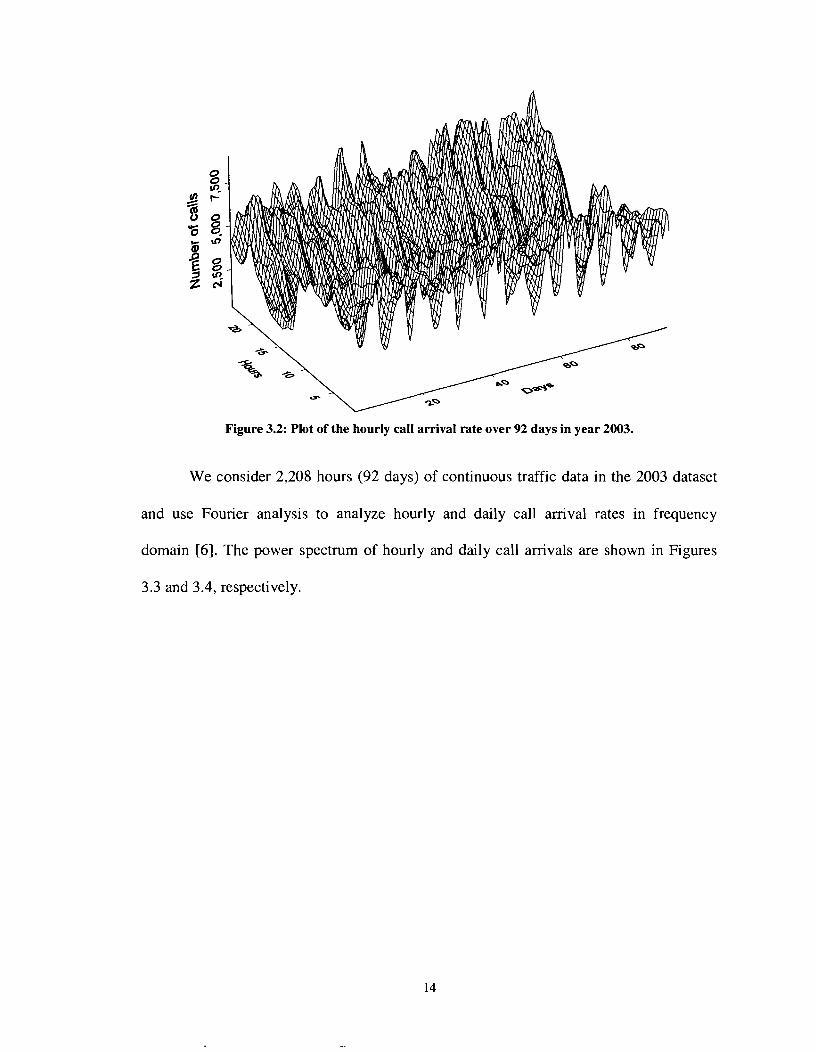
Figure 3.2: Plot of the hourly call arrival rate over 92 days in year 2003.

We consider 2,208 hours (92 days) of continuous traffic data in the 2003 dataset

and use Fourier analysis to analyze hourly and daily call arrival rates in frequency

domain [6]. The power spectrum of hourly and daily call arrivals are shown in Figures

3.3 and 3.4, respectively.

100 150 Period (hours)

Figure 3.3: Power spectrum of hourly call arrival from the 2003 dataset indicates a strong daily cyclic pattern.

I I

\ I I

20 40 60 Period (days)

Figure 3.4: Power spectrum of daily call arrival from the 2003 dataset indicates a strong weekly cyclic pattern.

Further analysis results shown in Figure 3.5 indicate that the busiest hour in a day

is around midnight, while the least amount of traffic is expected between 2 pm and 3 pm.

Furthermore, Thursday is the busiest day of a week, while Monday has the least number

of calls, as shown in Figure 3.6.

The observations of the cyclic patterns of the call arrival rates are important

because they provide useful guidelines for the E-Comm operators to schedule regular

network maintenance tasks, such as database backup, to be performed when the network

has least traffic.

Figure 3.5: Average hourly call arrival rate over 24 hours.

Figure 3.6: Average daily call arrival rate over seven days.

- - j - - -1 - - - - - I I

3.2.2 Call holding time

We also analyze the hourly average of call holding time (call duration). As shown

in Figure 3.7, call holding time does not demonstrate a strong cyclic pattern.

r - - - - - I - - - - - , I I :- - I I I I I I I I I

Figure 3.7: Hourly average of call holding time over 92 days in year 2003.

- 2002 Data -+- 2003 Data

sat. sh. MA". ~ ;e . wed. Thu. ~;i. Time (days)

We use Fourier analysis to analyze the hourly average of call holding time in the

frequency domain. Analysis results shown in Figure 3.8 indicate that the average hourly

call holding time has a weekly cyclic pattern.

Period (hours)

Figure 3.8: Power spectrum of average hourly call holding time indicates a weekly cyclic pattern.

3.2.3 Agencies and call arrival rates

The E-Comm network currently serves over ten emergency agencies including

Vancouver Police, RCMP, and BC Ambulance. Each emergency agency has a unique

agency ID. In this thesis, we use agency IDS to represent emergency agencies. The

mapping between agency ID and agency name is not disclosed due to security concerns.

Emergency agencies and their average daily call arrival rate are listed in Table

3.2. We can observe that few heavy user agencies account for most of the call traffic in

the E-Comm network. For example, call traffic generated by Agencies 2 and 5 accounts

for more than 80% of the overall traffic in both 2002 and 2003. The call traffic increasing

rates vary significantly among user agencies.

Table 3.2: Agencies and average daily call arrival rates.

I Agency ID I Average daily call arrival rate I Change

I I Year 2002 I Year 2003 1

The difference of call arrival rates among user agencies suggests that modeling

call traffic on agency level is more accurate than modeling traffic for the entire network.

Moreover, heavy user agencies should receive additional attention in traffic modeling.

2 1

Total

3.2.4 Systems and call arrival rates

The E-Comm network consists of eleven systems. E-Comm system IDS and

average daily call arrival rate of each system are listed in Table 3.3. Table 3.3 indicates

c1

68,462

2,999

95,184

n/a

39%

that the overall call traffic increased by 37% from 2002 to 2003, which implies that

additional channels are required in 2003 in order to maintain the same Grade of Service

(GoS). We can also observe that the change of average daily call arrival rate in different

systems varies significantly, which implies that each system needs individual assessment

when expanding its wireless channels.

Table 3.3: Systems and average daily call arrival rates.

I System 1 Average daily call arrival rate I Change

( 1 I Vancouver 1 53,183 1 56,736 1 7%

I

I 5 -1 ~eymour I

ID

2

3

4

1 6 1 Port Coquitlam I 15,336 ( 22,673 1 48%

Year 2002 Coverage

1 7 1 Richmond I 18,752 1 23,846 ( 27%

Year 2003

Burnaby

Maple Ridge

Langley

1 8 1 Mission 1 5,929 1 5,706 1 -4%

19,581

7,050

7,705

I 11 I Bowen Island I 7,960 1 4,021 1 -49%

9

10

27,325

8,263

18,354

3.3 Busy hours

PSWNs are designed to meet the GoS standards during busy hours. Industry

Canada requires that less than 3% of calls could be queued for an average call holding

time during busy hours [7].

40%

17%

138%

Surrey

South Surrey

Total

The average hourly call arrival rates for the 2002 and 2003 datasets are 2,853 and

3,966, respectively. Table 3.4 shows that the call arrival rate during busy hours is

12,714

7,288

159,740

31,953

13,969

21 8,171

151%

92%

37%

approximately twice the average call arrival rate. For the statistical modeling of call

traffic, we only consider busy hour traffic.

Table 3.4: The top three busiest hours in 2002 and 2003 traffic datasets.

Busy hour (BH) I Period I Number of calls

CHAPTER 4: STATISTICAL TRAFFIC MODELING

In this Chapter, we first introduce the modeling/simulation approach and describe

traditional models for evaluating radio networks. We then describe the process of

modeling call holding time and call inter-arrival time. We also address the call coverage

issue in the E-Comm network. Two statistical modeling techniques, the Kolmogorov-

Smirnov goodness-of-fit (K-S GoF) test and the Maximum Likelihood Estimation

(MLE), are also described.

4.1 Modeling/simulation approach

It is important to precisely estimate the maximum network capacity of public safe

wireless networks and predict network performance in the future. In other words, it is

important for the network operators to know answers for questions such as "How many

mobile radios we can put into our network while keeping the busy hour call blocking

probability under three percent?" and "How many additional channels are needed when

call volume is increased by twenty percent?"

Generally speaking, there are four approaches to study a system and to answer

these questions [S]: (1) experiment with the deployed system, (2) experiment with a

physical model of the system (test bed), (3) use an analytical approach to experiment with

a mathematical model of the system, and (4) use simulation to experiment with a

mathematical model of the system.

There are three ways to evaluate and predict the E-Comm network performance:

utilize existing formulas, employ a modeling/analytical approach, andlor use a

modeling/simulation approach. E-Comm operators currently use existing formulas such

as Erlang B and Erlang C to evaluate their network performance. However, we will show

in Section 4.2 that this approach has several limitations and cannot provide reliable

estimation results.

One way to predict future network traffic is to study the past traffic and extract

past patterns and relationships. These patterns and relationships form a model. The

modeling process provides a means of creating simplified representations of the "real

network". Once the mathematical model of the target network is built, we may either use

an analytical approach or a simulation approach to evaluate and predict the network

performance. In this thesis, we adopt the modeling/simulation approach because of its

capability to handle complex mathematical models.

To build the E-Comm traffic model, we first study the traffic data collected from

the E-Comm network. We then select several candidate distributions, estimate their

parameters, identify the most suitable distribution, and build a statistical model that

represents the usage of the E-Comm network.

4.2 Introduction to traditional traffic models

4.2.1 Erlang models

Erlang B and Erlang C models are widely used by call traffic engineers to plan the

network resources, such as number of phone lines in Public Switched Telephone Network

(PSTN), Private Branch Exchange (PBX) capacity of call centers, and number of radio

channels in cellular networks [lo]. Erlang models are named after the Danish

mathematician A. K. Erlang.

Erlang is used as a dimensionless unit in traffic engineering to measure traffic

intensity. It measures continuous use of one circuit. For example, call traffic generated by

a one hour long call is one Erlang. Call traffic generated by two 30 minutes long calls is

also one Erlang.

Mathematical representations of Erlang B and Erlang C models are given by

Equations (4-1) and (4-2), respectively. In both equations, N is the total number of

resources in the system, such as channels or lines, and A is the total traffic volume

measured in Erlang.

In Erlang B model:

AN

PB is the probability that a call request will be rejected due to lack of resources.

In Erlang C model:

N ! N - A P~ = N-I A X AN N ' 5--4-- 2 X ! ' N ! N - A

PC is the probability that a call request will be delayed in obtaining a resource.

Erlang B and Erlang C models assume (I) infinite number of call sources or that

the number of call sources is much larger than the number of available channels, (2)

Poisson distributed call arrival, and (3) exponentially distributed call holding time. The

Erlang B model further assumes that (4) a blocked call will be rejected immediately and

(5) a user will not retry the same request after being rejected. The Erlang C model further

assumes that (6) a blocked call will be put into a FIFO queue with infinite size and that

(7) a user will not abandon the call request until the call is successfully completed.

4.2.2 Failure of Erlang models

In the E-Comm network, although assumptions (1) and (2) are likely to be valid,

assumptions (3) through (7) are not applicable. Moreover, Erlang models were originally

developed for traditional networks where there is no group call, which implies that caller

and callee have a one-to-one relationship. However, calls in the E-Comm network are all

group calls (one-to-many caller-to-callee relationship) and most calls use more than one

channel simultaneously. These indicate that Erlang models are not suitable for the E-

Comm network.

4.3 Traffic modeling on agency level

We showed previously in Table 3.2 that the majority number of calls is initiated

by few user agencies. We further investigate the number of calls made by each agency

during the top three busiest hours in 2002 and 2003 datasets.

Table 4.1: Aggregated number of calls during the top three busiest hours in 2002 and 2003.

Table 4.1 indicates that during busy hours, more than 80% of the calls are

initiated by Agencies 2 and 5. Since these two heavy user agencies have larger impact on

the network than the remaining of the agencies, to simplify the traffic modeling process,

we regroup the agencies into three new agencies and model their call traffic. Table 4.2

shows the mapping between the original and the new agency IDS.

21

Total

Table 4.2: Regrouped agencies and the original agencies.

0

16,322

Virtual agency ID

A

B

C

0.0%

100%

Original agency ID

2

5

(all other agencies)

598

26,057

2.3%

100%

4.4 Modeling call holding time

Before we start describing the modeling of call holding time, we introduce two

related statistical modeling techniques: Kolmogorov-Srnirnov goodness-of-fit (K-S GoF)

test and Maximum Likelihood Estimation (MLE).

4.4.1 Maximum likelihood estimation

Introduced by R. A. Fisher in 1920s, MLE [9] is currently the most popular

method of estimating distribution parameters. The goal of MLE is to find the parameters

that make the candidate distribution fit the observed data best.

Let fo (x) = f (x 1 8) be the probability distribution function, where

8 = (8, , B, , ..., 8, ) is the parameter vector. Likelihood of B is defined as

Since the maximum product is difficult to calculate and logarithm is an increasing

function, we use the log-likelihood l(8) instead. The parameter /3 that maximizes l(0) will

also maximize like(@:

We use the Poisson distribution as an example to demonstrate how MLE works.

The Probability Density Function (PDF) for the Poisson distribution is

The log-likelihood can be deduced as

To find the maximum of 1(8), we final its derivative and set it to zero:

Equation (4-6) impliesR = X . However, in most other cases, E(8) is not deducible

mathematically. We use a software tool called rnle [12] to estimate the parameters.

4.4.2 Kolmogorov-Smirnov goodness-of-fit test

Goodness-of-fit test (GoF) is used to statistically verify whether or not a sample

dataset XI, X,, ..., X n follows a particular distribution with distribution function F. In

other words, the GoF test is used to test the following null hypothesis Ho:

&: X,, X , , ..., X , are independent random variables with a specific distribution

F ( 4 .

The Chi-square test [13] and the Kolmogorov-Smirnov test [13] are the most

popular goodness-of-fit tests. The Chi-square test is suitable for testing discrete random

variables, while the K-S test is more suitable for testing continuous random variables.

Since our objects (call holding time and call inter-arrival time) are both modeled using

continuous random variables, we use the K-S test.

The K-S GoF test is based on the empirical distribution function F,. Suppose that

we have n independent random variables XI, X,, ..., Xn . Since the order of these variables

does not affect the underlying distribution function, we further assume that

XI, X,, ..., Xn are in an increasing order. The Empirical Distribution Function (ECDF)

Fe is defined as:

total number of i where I x Few =

n

The Kolmogorov-Smirnov test statistic D is defined as:

D = supremum 1 F, (x) - F (x)l X

= ~ u ~ r e m u m { ~ u ~ r e m u m { F, (x) - F (x)} , supremum { F (x) - F, (XI}} (4-8)

Equation (4-8) states that a large value of D indicates a poor fit of Fe(x) and F(x). p-value,

defined as p-value = P, {D 2 d} [ l l ] , is an indicator of how likely F(x) is accepted. Null

hypothesis Ho is likely to be accepted when p-value > 0.01 and Ho is very likely to be

accepted when p-value > 0.05.

4.4.3 Survey of existing models for call holding time

Over the years, a number of probability models have been developed for call

holding time in various networks such as PSTN and cellular networks. Bolotin shows

1141 that the exponential distribution underestimates the proportion of short calls in

traditional PSTNs. Bolotin further shows [15] that the call holding time in traditional

PSTNs follows lognormal distribution with a mean value of 200-300 seconds. In [16]-

[19], Jordan and Barcel6 show that Erlang-jk and mixture of lognormals fit very well

voice holding time in Public Access Mobile Radio (PAMR) systems with mean value of

2 0 4 0 seconds. Using field data from cellular telephony systems, Jedrzycki and Leung

find that the lognormal distribution provides a better fit for the channel holding time [20].

In [21], [22], Orlik and Rappaport proposed a model called the Sum of the Hyper-

Exponential (SOHYP) to model the channel holding time in data used in [20]. Fang et al.,

proposed the Hyper-Erlang distribution [23]-[25] to model cell residence time that may

be used to better characterize channel holding time in mobile computing and Personal

Communication Services (PCS) networks.

Traffic data from PSWNs are rarely available due to their confidential nature and,

hence, few models of call holding time have been developed for such networks. The large

difference between mean call holding times in PSWNs and call holding times in

PSTNICellular networks suggests that call holding time models developed for other

networks might not be suitable for PSWNs. A recent study of E-Comm's aggregated

traffic shows that the call holding time during busy hours fits the lognormal distribution

[27]. However, to the author's knowledge, there is no published work dealing with

modeling call traffic in PSWNs on user agency level.

4.4.4 Model comparison and selection

In this Section, we investigate the call holding time of E-Comm traffic on the user

agency level. The candidate distributions to be tested and their PDFs are listed in

Table 4.3.

Table 4.3: Candidate distributions for call holding time.

I Distribution I Probability density function

Exponential

Lognormal

To fit and compare candidate distributions with E-Comm traffic data, we first

extract 500 sequential data samples (call holding times) from the traffic data table. We

then select a candidate distribution and use MLE to estimate its parameters. The K-S GoF

test is then used to evaluate the candidate distribution. When p-value is greater than 0.03,

the candidate distribution is likely to be accepted. Otherwise, the candidate distribution is

likely to be rejected.

1 -; f ( x ) = -e a

1 (W-P)~ f ( x ) = -2g2

x 2no

Gamma

We fit candidate distributions with call holding times of Agencies A, B, and C

during the top three busiest hours in the 2002 dataset. Estimated distribution parameters

and K-S test results are listed in Table 4.4. Cells with p-value > 0.03 are marked in grey.

K-S test results (p-values) shown in Table 4.4 indicate that the lognormal distribution is

ideal to model the call holding time for Agency A.

- I -t f ( x ) = P-' - e

( k - I ) !

Table 4.4: Test of candidate distributions for call holding time of Agency A during busy hours in the 2002 dataset.

Distributions

Exponential

K-S test results shown in Table 4.5 indicate that although the lognormal

distribution does not fit the call holding time of Agency B at 3% significance level all the

time, it is nevertheless adequate to model it call holding time.

Gamma

Table 4.5: Test of candidate distributions for call holding time of Agency B during the top three busy

Distribution parameters and K-S test results

hours in the 2002 dataset.

Busy hour 1

P = 3683.6

p-value = 0

P = 1 108.0657 k = 3.3246 p-value = 0.0002

Exponential

Busy hour 2

P = 3664.06

p-value = 0

P=1173.6163 k = 3.1222 p-value = 0.01 37

Distributions

Lognormal

Busy hour 3

P = 3658.56

p-value = 0

P=1493.315 k = 2.4501 p-value = 0.0027

Gamma


P = 4269.78 p-value = 0

Busy hour 1

P = 41 98.82 p-value = 0

P = 3742.3 p-value = 0

Busy hour 2 Busy hour 3

K-S test results shown in Table 4.6 indicate that no candidate distribution fits the

call holding time of Agency C at satisfying significance levels. However, the lognormal

distribution still performs better than other candidate distributions.

P = 21 41.4626 k = 1.994 p-value = 0

P = 2002.4384 k = 2.097 p-value = 0.001 2

P = 181 1.9239 k = 2.0655 p-value = 0.0001

Busy hour 2 Busy hour 3

p-value = 0 p-value = 0

Table 4.6: Test of candidate distributions for call holding time of Agency C during the top three busy hours in the 2002 dataset.

Because the two heavy user agencies (Agencies A and B) account for 80-90% of

the total call traffic and their call holding time follows lognormal distribution, we adopt

the lognormal distribution to model call holding time in simulations.

Distributions

Exponential

Lognormal

Gamma

a = 8.094 p = 0.6228

p-value = 0.0036

P = 1539.01 57 k = 2.6087

p-value = 0

4.5 Modeling call inter-arrival time


Busy hour 1

P = 3505.58 p-value = 0

a = 7.8759 p = 0.81 54

p-value = 0

P = 1848.561 9

k = 1.8965 p-value = 0

-- --

a = 7.9621 p = 0.7251

p-value = 0.0002

P = 1938.2806 k = 1.9538 p-value = 0

4.5.1 Survey of existing models for call inter-arrival time

The Poisson model for call arrival time is widely used in PSTNs [28]. It implies

that the inter-arrival time is exponentially distributed. Exponentially distributed call inter-

arrival time was originally assumed in cellular networks. It was shown [29]-[31] that

exponential distribution is only suitable for modeling inter-arrival times of "fresh" (new)

calls in micro-cellular networks. However, exponential distribution is not suitable for

modeling all (new and hand-over) call inter-arrivals in micro-cellular networks due to the

frequent call handovers.

The E-Comm network is a macro-cellular network where call handover rarely

happens. Call inter-arrival time in the E-Comm network was found to be exponentially

distributed [27].

4.5.2 Model comparison and selection

In this Section, we investigate the call inter-arrival time of E-Comm traffic on the

user agency level. Candidate distributions are listed in Table 4.7.

Table 4.7: Candidate distributions for call inter-arrival time.

Exponential

Lognormal r- Gamma L

Probability density function

X k - l -5

f ( x ) = pk -- e ( k -I)!

The method we employ to evaluate candidate distributions of call inter-arrival

time is similar to the method used to evaluate call holding time. Estimated distribution

parameters and K-S test results are listed in Tables 4.8-4.10. Cells with p-value > 0.03

are marked in grey.

The results shown in Tables 4.8 and 4.9 indicate that both exponential distribution

and gamma distribution are adequate to model the call inter-arrival time of Agencies A

and B. This is expected since the gamma distribution is a more general form of

exponential distribution. We use the exponentially distributed call inter-arrival time in

later simulations because of its simplicity.

Table 4.8: Test of candidate distributions for call inter-arrival time of Agency A during the top three

Distributions

Exponential

Lognormal r- Gamma L

busy hours in the 2002 dataset.


Table 4.9: Test of candidate distributions for call inter-arrival time of Agency B during the top three busy hours in the 2002 dataset.

Busy hour 1

a = 6.6043 p = 1.0791 p-value = 0.0001

Lognormal

Busy hour 2

a = 7.0211 p = 1.2888 p-value = 0.0002

Distributions

Busy hour 3

a = 6.6795 p = 1 .I643 p-value = 0.0009


Busy hour 1 I Busy hour 2 I Busy hour 3

Results shown in Table 4.10 indicate that although Gamma distribution may

= 7.1 558 p = 1.0865 p-value = 0.001 7

occasionally model the distribution of call inter-arrival time of the light user Agency C,

no candidate distribution is likely to be accepted. We assume exponentially distributed

o = 6.72 p = 1.2406 p-value = 0.01 03

call inter-arrival time for Agency C in simulations because Agency C accounts for only

o = 6.8838 p = 1.2564 p-value = 0.0007

approximately 10% of the call traffic and has much less impact on E-Comm network than

Agencies A and B.

Table 4.10: Test of candidate distributions for call inter-arrival time of Agency C during the top three busy hours in the 2002 dataset.

4.6 Call coverage pattern

The call coverage pattern is important in simulating the E-Comm network

because all calls in the E-Comm network are group calls and most of them cover more

than one system. As previously discussed in Section 2.1.6, we might underestimate the

call blocking probability if we ignore the group calls and investigate only one system.

The call coverage pattern in the E-Comm network is largely determined by the

organizations of talk groups and the radio device deployment of user agencies. Factors

that affect the call coverage pattern are unknown. In simulations of the E-Comm network,

we assume that the pattern of call coverage and the corresponding probability of

occurrences remain unchanged. A sample of call coverage pattern is shown in Table 4.11.

Table 4.11: A sample of call coverage pattern of Agency A during the top three busy hours in 2003.

Call coverage I NO. of occurrences I Percentage I System No. 1, 2, 3

System No. 1, 3, 8, 10, 1 1

System No. 3, 5, 7, 9, 10

. . .

45

69

1.35%

2.07%

236

... 7.08%

. . .

CHAPTER 5: WARNSIM: A SIMULATOR FOR PSWN

In this Chapter, we introduce the design, implementation, and validation of

WarnSim.

5.1 Overview

Several network simulation tools are currently available for simulating packet

switched networks: OPNET [32], ns-2 [33], and J-SIM [34]. However, to the author's

knowledge, there is no simulation software tool publicly available for simulating circuit

switched networks such as PSWNs. Moreover, it is inefficient to use a simulator designed

for packet switched networks to mimic and simulate circuit switched networks. Hence,

we developed WarnSim, an effective, flexible, and easy to use simulation tool to simulate

PSWN systems.

WarnSim is a publicly available tool designed to simulate circuit switched radio

networks [35], [36]. It can simulate various network sizes (number of cells in a network)

and cell capacities (number of channels in cells). Traffic traces are easily imported or can

be modeled with a variety of statistical distributions. These features make WarnSim

preferable for simulating wide area radio networks, such as PSWNs.

WarnSim is developed using Microsoft Visual C# .NET, which has a comparable

performance to Java [37]. WarnSim works on Windows platforms with .NET framework

support and comes with a graphical user interface.

5.2 Modules and call flowchart

WarnSim consists of seven modules, shown in Figure 5.1.

-1 1 Simulation

WarnSim

I module 1 I configuration module I (a)

Simulation statistics module

Network module

Simulation Simulation process module configuration 1 module 1 I I I \

\

Simulation process module

Call admission control module P

Random variable module

Simulation variable module statistics module

I I \ I \ A

Figure 5.1: WarnSim: (a) module hierarchical diagram and (b) relationship diagram.

Network module models the cells of a PSWN. A network module may consist of

Call traffic module

several cells. Each cell has one or more channels with the attribute "busy duration". A

f--)

channel is free if its "busy duration" is zero. Otherwise, the channel is occupied for the

Network module

Call admission control module

duration of time specified by the "busy duration". The network module distributes calls to

)

cells, tracks the status of the system (number of free or occupied channels), and

periodically updates the channel status in every cell.

Call trafJic module prepares call traffic for simulation. It can import traffic trace

files from text filesldatabases or generate call traffic based on user-defined distributions

and combine them during a single simulation run.

Call admission control module uses the calls from the call traffic module and

checks with the network module to determine if there are available channels for a call to

be established. It also manages the retrying mechanism of blocked calls.

Simulation configuration module keeps track of call queuing mechanism and

parameters, such as the maximum call queuing time, simulation duration, and simulation

granularity.

Simulation process module uses a global timer to control and synchronize the

operation of the WarnSim modules.

Simulation statistics module collects real-time and summary statistics (number of

calls, blocked calls, call blocking probability, channel utilization, cumulative number of

calls, cumulative blocked calls, cumulative call blocking probability, and cumulative

channel utilization) from other modules. It is also used to display and visualize simulation

results.

Random variable module generates random numbers and random variables. We

adopted the MT random number generator [38], which is suitable for stochastic

simulations. We also implemented seven types of random variables: uniform,

exponential, gamma, normal, lognormal, loglogistic, and Weibull.

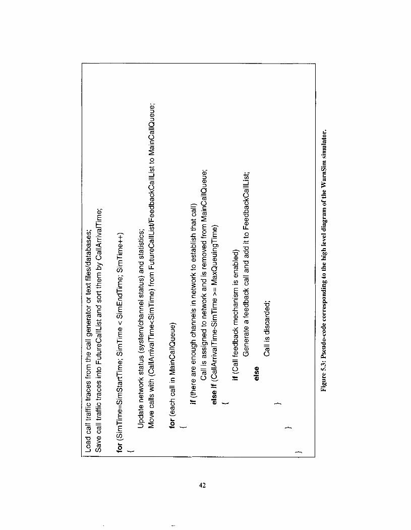
A high level diagram illustrating the call flow mechanism of WarnSim is given in

Figure 5.2. The basic functionality of WarnSim is described by the pseudo-code, as

shown in Figure 5.3.

Load

cal

l tra

ffic

trac

es fr

om th

e ca

ll ge

nera

tor o

r te

xt fi

lesl

data

base

s;

Sav

e ca

ll tr

affic

trac

es in

to F

utur

eCal

lLis

t and

sor

t the

m b

y C

allA

rriv

alT

ime;

for

(Sim

Tim

e=S

imS

tart

Tim

e; S

imT

ime

< S

imE

ndT

ime;

Sim

Tim

e++)

Upd

ate

netw

ork

stat

us (

syst

emlc

hann

el s

tatu

s) a

nd s

tatis

tics;

M

ove

calls

with

(C

allA

rriv

alT

ime<

Sim

Tim

e) fr

om F

utur

eCal

lLis

t/Fee

dbac

kCal

lLis

t to M

ainC

allQ

ueue

;

for

(eac

h ca

ll in

Mai

nCal

lQue

ue)

{ if

(th

ere

are

enou

gh c

hann

els

in n

etw

ork

to e

stab

lish

that

cal

l) C

all i

s as

sign

ed to

net

wor

k an

d is

rem

oved

from

Mai

nCal

lQue

ue;

else

if (

Cal

lArr

ival

Tim

e-S

imT

ime

>= M

axQ

ueui

ngT

ime)

{ if

(C

all f

eedb

ack

mec

hani

sm is

ena

bled

) G

ener

ate

a fe

edba

ck c

all a

nd a

dd it

to F

eedb

ackC

allL

ist;

else

C

all i

s di

scar

ded;

Fig

ure

5.3:

Pse

udo-

code

cor

resp

ondi

ng to

the

high

leve

l dia

gram

of t

he W

arnS

im s

imul

ator

.

5.3 WarnSim simulation steps

Most simulations with WarnSim include five main steps:

Step 1: Network topology setup

addremovelconfigure systems

loadlsave network topology

Step 2: Traffic sources setup

addremovelconfigure traffic sources from a text file or a database

add/remove/configure call traffic generators

loadsave traffic sources

Step 3: Simulation parameters configuration

configure the length (time span) of simulation

configure calls queuing mechanism

configure dropped calls retrying mechanism

configure statistics collection interval

Step 4: Run simulation

runlstop simulation

pause simulation to view intermediate simulation results

Step 5: Analyze simulation results

listlsave simulation results

plotlexport simulation results.

5.4 WarnSim interface

WarnSim includes a graphical user interface. Figures 5.4-5.8 show four WarnSim

screens during a simulation experiment. Systems in WarnSim are configured in a star

network topology, as shown in Figure 5.4 (a). Figure 5.4 (b) shows the WarnSim network

configuration screen capturing network information (cells and number of channels). A

popup window used to configure the system ID, system name, and number of channels is

also shown in Figure 5.4 (b). Figures 5.5 and 5.6 show the configuration screens for

traffic sources. A list of traffic sources and popup windows used to

import/generate/configure traffic traces are also shown. Figures 5.7 (a) and (b) capture

the simulation results screens for channel utilization vs. simulation time. Figures 5.8 (a)

and (b) show the simulation results for discarded calls vs. simulation time.

System 2 system N

Figure 5.4: WarnSim: (a) network topology and (b) network configuration screen.

Figure 5.5: WarnSim traffic source configuration screen: importing traffic.

Figure 5.6: WarnSim traffic source configuration screen: generating traffic.

WarnSim simulation results

Syslem 1 Aoencv AJll

0 100 200 300 400 500 600 700 Simulation time (sec)

WarnSim simulation results

I - System 1 Agency AJl]

. . . . . . . . . . . . , . .

0 100 200 300 400 500 600 700 Simulation time (sec)

Figure 5.7: WarnSim simulation results screens for channel utilization of Vancouver system during: (a) a sample week in 2002 and (b) a sample week in 2003. The graphs show the running average

calculated over ten-minute intervals.

WarnSim simulation results [ - System 1 Agency All1

. . . . . . . . . . . . . . . . . . . . . . . . . . . . . . .

. . . . . . . . . . . . . . . . . . . . . . . . . . . . . . . . . . . . . . . . . . . . .

. . . . . . . . . . . . . . . . . . . . . . . . . . . . . . . . . . . . . . . . . . . . . . . . . . . . . . . . . . . . . . . . . . . . . . . . . . . .

. . . . . . . . . . . . . . . . . . . . . . . . . . . . . . . . . . . . . . . . . . . . . . . . . . . . . . . . . . . . . . . . . . . . . . . . . . . . . . . . .

. . . . . . . . . . . . . . . . . . . . . . . . . . . . . . . . . . . . . . . . . . . . . . . . . . . . . . . . . . . . . . . . . . . . . . . . . . . . . . . . . . . . . -

. . . . . . . . . . . . . . . . . . . . . . .

. . . . . . . . . . . . . . . . . . . . . . . . . . . . . . . . . . .

i 0 100 200 300 400 500 600 700

Sirnubtion time (sec)

WarnSim simulation results - System 1 ~gency All] 35- . . . . . . . . . . . . . . . . . . . . . . . . . . . . . . . . . .

30 -- . . . . . . . . . . . . . . . . . . . . . . . . . . . . . . . . . . . . . . . . . . . . . . . . .

a 25 1: .. . . . i

i /-'--: - - . . . . . . . . . . . . . . . . . . . . . . . . . . . . . . . . . . . . . . . . . . . . . . . .

z li x g 20 :: . . . . . . . . . . . : . . . . . . . . . . . . . . . . . . . . . . . . . . . . . . . . . . . . . . . . . . . . . . . . . . . . . r . . . . . . . . . . . : - D ::

. . . . . . . . . . . . . . . . . . . . . . . . . . . . . . . . . . . . . . . . . . . . . . . . . . . . . . . . . . . . . . . . . . . . . . . . . g 15 :r .:. :. .: - .. - - gl0::... . ; . . . . . . > . . . . . . : d : . . . . . . ; . . . . . . : 0 .-

5 r-. . . . . . . . . . . . . . . . . . . . . . . . . . . . . . . . . . . . . . . . . . . . . . . . . . . . . . . . . .-

j / o r ; ; ~ ~ i : . ! , : ~ > : : i : : ; ~ i : : : : : : ; : ~ ! : ; ; , I 0 100 200 300 400 500 600 700

Simulation time (sec)

Figure 5.8: WarnSim simulation results screens for the cumulative number of blocked calls in Vancouver system during: (a) a sample week in 2002 and (b) a sample week in 2003.

5.5 Validation of WarnSim simulator

We performed several steps to validate WarnSim. We first use build-in K-S GoF

functions provided by MATLAB [39] and S-PLUS [40] to test the random variable

generator implemented in WarnSim. All K-S GoF tests return high p-values (> 0.1),

which validates the WarnSim generated random variables.

We then use various artificial testing traces to validate the deterministic WarnSim

modules, such as call admission control module and simulation statistics module. A

simple example of the testing scenario is to let 11 calls simultaneously reach a system

with 10 channels. As expected, one call will be queued due to the lack of a free channel.

We further validate WarnSim by comparing the prediction results of Erlang B

model with WarnSim simulation results. As shown in Table 5.1, call blocking

probabilities match very well.

Table 5.1: Comparison of call blocking probability predicted by Erlang B model and the WarnSim simulated call blocking probability.

I I Erlang B model I WarnSim I I Network configuration 1 10 phone lines I 1 system with 10 channels I

Call traffic volume

Call holding time

Call inter-arrival time

Call blocking probability

10 Erlangs

exponentially distributed

Dealing with blocked calls

17% - 27%; average=21.86% (1 0 simulation runs)

10 Erlangs

exponentially distributed with mean value of 180 seconds

exponentially distributed exponentially distributed with mean value of 18 seconds

blocked calls neither queued nor retried

Max Queuing Time = 0; blocked calls are not retried

5.6 Scalability and performance of WarnSim

WamSim provides good flexibility in choosing the network size (the number of

cells in the network) and cell capacities (the number of channels in each cell). In our

simulation experiments, WarnSim successfully handled sample networks with 100 cells

and 50 channels in each cell. They are approximately ten times larger than the size of the

E-Comm network and are sufficient to model any deployed PSWNs.

WarnSim simulation tests are performed on a windows workstation equipped with

Intel Pentium 4 2.8GHz CPU and 5 12Mbyte memory. The operating system is Microsoft

Windows XP Professional with .NET framework 1.1 supports. On this platform, a

simulation with one hour of busy hour traffic from the E-Comm PSWN lasts less than

one minute. The high performance of WarnSim enables users to quickly test various

network configurations and call traffic, and to efficiently perform trace driven

simulations and evaluate network performances during busy hours.

CHAPTER 6: SIMULATION AND PREDICTION

In this Chapter, we use WarnSim to validate the proposed traffic model and to

evaluate and predict E-Comm network performance.

6.1 Validation of the proposed traffic model

To validate the proposed traffic model, we first use WarnSim to generate traffic

traces and compare them with the collected E-Comm traffic data. WarnSim distribution

parameters listed in Table 6.1 are used for the call generator to model busy hour traffic of

the 2003 dataset.

Table 6.1: Distribution parameters for the WarnSim call generator.

Call holding time


Agency A I Agency B

Lognormal

a = 8.05 p = 0.55

lognormal

a = 7.88 p = 0.82

lognormal

a = 8.09 p = 0.73

Exponential p = 1354

exponential exponential p = 761

In the simulation scenarios, systems and channels shown in Table 6.2 reflect the

configuration of the E-Comm network during the busiest hour in 2003.

Table 6.2: System IDS and number of channels.

SystemID

Channels

3

4

1

10

2

7

4

5

5

3

6

7

7

8

8

4

9

7

10

6

11

3

Simulation results listed in Table 6.3 indicate that the proposed traffic model

performs adequately when used to evaluate call bloclung probability and channel

utilization in the E-Comrn network.

Table 6.3: Comparison of network performance: using collected traffk (actual) vs. model generated traffic (simulated).

Evaluation of E-Comm network performance

System ID

We can evaluate the Grade of Service (GoS) of PSWN by performing WarnSim

simulations using genuine traffic data. In this Section, we first describe the simulation

scenarios and source traffic traces. We then describe the evaluation results of two GoS

standards in the E-Comm network: call bloclung probability and channel utilization.

6.2.1 Network performance during busy hours

Three simulation scenarios are setup to evaluate the GoS of the E-Comm network

during the top three busiest hours in 2003. Systems and channels reflect the

Actual blocking

probability ("/.I

Actual channel

utilization ("/.I

Simulated blocking

probability ("/.I

Simulated channel utilization

("/.I

corresponding configurations of the E-Comm network, as shown in Table 6.4. The source

traffic traces are extracted from the top three busiest hours in 2003 dataset and are

transformed into the format shown in Table 3.1. Maximum queuing time of blocked call

is set to zero. Simulation statistics including channel utilization, total number of calls,

number of blocked calls, and call blocking probability for each system are collected by

WarnSim. Simulation results shown in Tables 6.5-6.7 indicate that System 1 is the

busiest system in the E-Comm network in terms of both hourly call arrival rate and call

blocking probability. Few calls may be blocked in Systems 2, 4, 6, 7, and 9. In other

systems, calls never got blocked and channel utilizations are relatively low.

Table 6.4: System IDS and number of channels during the top three busy hours in the 2003 dataset.

System ID No. of channels in busy hour 1

No. of channels in busy hour 2

No. of channels in busy hour 3

Table 6.5: Simulation results of the busiest hour in the 2003 dataset.

Table 6.6: Simulation results of the second busiest hour in the 2003 dataset.

I System ID Channel utilization

Total No. of calls

No. of blocked calls

Blocking Probability

6.2.2 Number of channels and Grade of Service

We now investigate the relationship between the number of available channels

and the GoS (channel utilization and call blocking probability). The second busiest hour

in 2003 dataset is chosen because it has the highest call blocking probability in System 1

among the top three busiest hours in the 2003 dataset. While keeping the number of

channels in the remaining systems unchanged, we vary the number of available channels

in System 1 from 1 to 14. WarnSim simulation results are collected from System 1. In

this scenario, the maximum queuing time of blocked calls is set to zero.

Table 6.7: Simulation results of the third busiest hour in 2003 dataset.

Simulation results shown in Table 6.8 and Figure 6.1 depict the relationship

between the number of channels and the call bloclung probability. When the number of

channels increases from 1 to 8, call blocking probability drops to 12% at a near constant

rate as shown in Figure 6.1. It then decreases slowly to zero when the number of channels

reaches 14. The channel utilization drops slowly when the number of channels increases

8

9

10

11

8%

37%

16%

6%

353

2,316

960

1 78

0

8

0

0

0.0%

0.3%

0.0%

0.0%

from 1 to 8 and then it drops at a constant rate. Based on these results, we can determine

the number of necessary channels in order to meet a certain Grade of Service.

Table 6.8: Relationship between number of channels, call blocking probability, and channel utilization. Maximum queuing time is set to zero.

No. of channels Channel utilization ("/.)

Blocking probability ("/.)

Figure 6.1: Relationship between number of channels, call blocking probability, and channel utilization. Maximum queuing time is set to zero.

6.2.3 Maximum queuing time and Grade of Service

An effective way to lower the call blocking probability without adding new

channels is using call queuing mechanism. The call queuing mechanism implies that

instead of dropping a call immediately after it failed to obtain a free channel, the call is

placed in a waiting queue for a certain amount of time. The call is dropped if it cannot get

the required channels after waiting for the amount of time specified by the maximum

queuing time.

We simulate scenarios where maximum queuing time increases from 0 to 1.5

seconds and collect call blocking probability statistics. The second busiest hour in the

2003 dataset is chosen for simulation. Simulation results shown in Table 6.9 and Figure

6.2 indicate that increasing the maximum queuing time can effectively lower the call

blocking probability. The call blocking probability of System 1 is lowered by more than

80% when the maximum queuing time is increased from 0 to 1 second.

Table 6.9: Maximum call queuing time vs. call blocking probability.

Maximum queuing time (ms)

0

Call blocking probability ("/.)

3.4

" 0 0.2 0.4 0.6 0.8 1 1.2 1.4 1.6 Maximum queuing time (sec)

Figure 6.2: Maximum call queuing time vs. call blocking probability.

6.3 Prediction of the E-Comm network performance

In this Section, we predict the E-Comm network performance in terms of call

blocking probability in cases of increased call traffic volume. Two case scenarios are

investigated. The system IDS and the number of channels for both scenarios are shown in

Table 6.10. The maximum queuing time in both scenarios is set to zero.

6.3.1 Simulation scenario one

We first consider a sample scenario where the number of calls made by Agency A

increases by 100% from the 2003 busy hours. WmSim distribution parameters for the

call generator are listed in Table 6.1 1.

Table 6.10: System IDS and number of channels.

System ID

Channels 3 1 0 7 4 5 3 7 8 4 7 6

1 2 3 4 5 6 7 8 9 1 0 1 1

Table 6.11: Scenario one: distribution parameters for the WarnSim call generator.

I Agency A I Agency B I Agency C 1

The simulation results shown in Table 6.12 indicate that the call blocking

Call holding time


probability of Systems 1 visibly increases after the call traffic increase.

Table 6.12: Comparison of network performance. Scenario one: using collected traffic (original) vs. model generated traffic after the increase (predicted). Cells with call blocking probability higher

than 3% are marked in grey.

Lognormal a = 8.05 p = 0.55

Exponential p = 677

Predicted channel utilization

W) 71 - 72

Further WarnSim simulations reveal that System 1 requires 4 additional channels

in order to maintain call blocking probabilities below the required 3% [7] .

lognormal a = 8.09 p = 0.73

exponential p = 761

lognormal a = 7.88 p = 0.82

exponential p = 3480

6.3.2 Simulation scenario two

We now consider the sample scenario where the number of calls made by Agency

B increases by 100% from 2003 busy hours. WarnSim distribution parameters for the call

generator are listed in Table 6.13.

Table 6.13: Scenario two: distribution parameters for the WarnSim call generator.

Call holding time

The simulation results shown in Table 6.14 indicate that the call blocking

probabilities of four systems (IDS 1, 2, 4, and 9) visibly increase after the call traffic

increase.


Further simulations reveal that in order to maintain call blocking probabilities of

all systems below 3%, Systems 1, 2, 4, and 9 require 4, 2, 1, and 3 additional channels,

respectively.

Agency A

Lognormal o = 8.05 p = 0.55


Agency B

lognormal o = 8.09 p = 0.73

Agency C

lognormal 0 = 7.88 p = 0.82

exponential p = 381


Table 6.14: Comparison of network performance. Scenario two: using collected traffic (original) vs. model generated traffic after the increase (predicted). Cells with call blocking probability higher

than 3% are marked in grey.

System ID Original blocking

probability ("/.I

Original channel

utilization ("/.I

Predicted blocking

probability ("/.I

Predicted channel utilization

("/.I

CHAPTER 7: CONCLUSIONS AND FUTURE WORK

In this Chapter, we conclude this thesis and describe possible future work.

7.1 Conclusions and contributions

In this thesis, we described the structure of the E-Comm network and the

collection of traffic data. We then analyzed the E-Comm traffic data and characterized its

properties such as the daily and weekly cyclic patterns of call arrival rate and call holding

time. We proposed a statistical model of call traffic on the user agency level. The

lognormal distribution proved to be appropriate for modeling call holding time, while the

exponential distribution was suitable for modeling call inter-arrival time. We also

addressed the call coverage issue of group calls.

In order to evaluate and predict the performance of the E-Comm network, we

developed a new simulation tool named WarnSim. With WarnSim simulations, we

validated the proposed traffic model and evaluated the performance of the E-Comm

network. We found that the E-Comm network is capable of handling busy hour traffic

based on the 2002 and the 2003 E-Comm traffic data. We predicted E-Comm network

performance in cases of increased call traffic volume. Simulation results showed that

when call traffic generated by E-Comm heavy user agencies increases by 100% during

busy hours, the E-Comm network was unable to maintain the required Grade of Service.

Further WarnSim simulations suggested the E-Comm network capacity (number of

channels in each system) needed to accommodate the increased call traffic.

7.2 Future work

The related network traffic prediction model, such as the cluster-based SARIMA

model developed by H. Chen [41], can be adopted to work with the proposed traffic

model and the WarnSim simulator to better predict future performance of the E-Comm

network.

WarnSim simulator may be improved and optimized. There are seven types of

random variables currently available in WarnSim. Additional random variables may be

added to WarnSim when needs arise. Furthermore, the internal algorithm of WarnSim

may be further optimized to achieve better performance in terms of simulation speed.

Ad hoc networks are self-organizing networks of user terminals that form without

the need for prior network infrastructure. Because of their adaptable, robust, and rapidly

deployable potentials, ad hoc networks are being considered for the next generation

PSWNs. In [42], D. Sharp proposed a multi-level hierarchical PSWN architecture that

uses a dominating-set based backbone network to interconnect geographically distributed

ad hoc networks in order to meet the needs of emergency communications. WarnSim

could be further developed and adopted to evaluate performance of the new generation

public safety wireless networks.

APPENDIX A: MAXIMUM LIKELIHOOD ESTIMATION (MLE) SCRIPTS

A.l MLE script for lognormal distribution

MLE

TITLE = "MLE for Lognormal distribution"

MAXITER = 500

EPSILON = 1E-10

DATAFILE("Sample.dat")

INPUT-SKIP = 0

DELIMITERS = " , "

OUTFILE("Result.out")

DATA

duration FIELD 1 DROPIF duration=O

END

MODEL

DATA

PDF LOGNORMAL(duration)

PARAM a

Low=o.oooo1

HIGH=5 0

START=0.05

END

PARAM b

LOw=o.oooo1

HIGH=5 0

START=0.05

END

END

END

RUN

FULL

END

END

A.2 MLE script for gamma distribution MLE

TITLE = "MLE for Gamma distribution"

MAXITER = 500

EPSILON = 1E-10

DATAFILE("Sample.datM)

INPUT-SKIP = 0

DELIMITERS = " , "

OUTFILE("Result.out")

DATA

duration FIELD 1 DROPIF duration=O

END

MODEL

DATA

PDF GAMMA(duration)

PARAM lambda

L0W=0.000001

HIGH=l

START=0.05

END

PARAM c

LOW=O. 001

HIGH=50

START=0.05

END

END

END

RUN

FULL

END

END

REFERENCES

SAFECOM Program. Public Safety Communications and Interoperability Statement of Requirements [Online]. Available: http://www.safecomprogram.govl files/PSCI-Statement-of-Requirements-v 1-0.pdf. Accessed: Aug. 15,2004.

SAFECOM Program. About SAFECOM [Online]. Available: http://www. safecomprogram.gov.

Emergency Communications for Southwest British Columbia Incorporated [Online]. Available: http://www.ecomm.bc.ca.

K. Bayne, 2000 operating budget: E-Comm and the Vancouver emergency [Online]. Available: http://www.city.vancouver.bc.cdctyclerWcclerk/O00420/ Csbl-4.htm. Accessed: Aug. 15,2004.

CornNet Ericsson. EDACS explained [Online]. Available: http://www. trunkedradio.net/trunked/edacs/EDACS-Whitepaper.pdf. Accessed: Aug. 15, 2004.

The Mathworks. Fourier analysis and the Fast Fourier Transform (FFT) [Online]. Available: http://www.mathworks.com/access/helpdes~techdoc/ math/datafun20.html. Accessed: Aug. 15,2004.

Industry Canada. Channel Loading Guidelines [Online]. Available: http://strategis.ic.gc.cdepic/intemet/in~mt-g~t.n~f/en/~f08015e.htm1. Accessed: Aug. 15,2004.

A. M. Law and W. D. Kelton, Simulation Modeling and Analysis, 3rd ed. Toronto, ON: McGraw-Hill, 2000, p. 4.

W. Gilchrist, Statistical Modelling. Toronto, ON: John Wiley & Sons, 1984, pp. 194-205.

Diagnostic Strategies. TrafJic modeling and resource allocation in call centers [Online]. Available: http:Nwww.diagnosticstrategies.com/traffic~modeling.htm. Accessed: Aug. 15,2004.

S. M. Ross, Simulation, 2nd ed. Toronto, ON: Academic Press, 1997, pp. 189-202.

D. J. Holman, Mle: a programming language for building likelihood models [Online]. Available: http://faculty.washington.edu/-djholman/mle. Accessed: Aug. 15,2004.

NISTISEMATECH. NZST/SEMATECH e-Handbook of statistical methods [Online]. Avai lable :h t tp : / /www.i t l .n is t .gov/div898/handboo~eda.pdf . Accessed: Aug. 15,2004.

V. A. Bolotin, "Modeling call holding time distributions for CCS network design and performance analysis," IEEE Journal on Selected Areas in Communications, vol. 12, no. 3, pp. 433438, April 1994.

V. A. Bolotin, "Telephone circuit holding time distributions," in Proc. of 14'~ International Teletrafic Congress (ITC'94), June 1994, pp. 125-134.

J. Jordan and F. Barcelo, "Statistical modelling of channel occupancy in PAMR systems," in Proc. of 1.5'~ International Teletrafic Congress (ITC997), June 1997, pp. 1169-1 178.

F. Barceld and J. Jordan, "Voice holding time distribution in trunked PAMR systems," in Proc. of IEEE Vehicular Technology Conference (VTC'97), May 1997, pp. 436440.

J. Jordan and F. Barceld, "Statistical modelling of transmission holding time in PAMR systems," in Proc. of IEEE Global Telecommunications Conference (GLOBECOM '97), Nov. 1997, vol. 1, pp. 121-125.

F. Barceld and J. Jordan, "Channel holding time distribution in public telephony systems (PAMR and PCS)," IEEE Trans. on Vehicular Technology, vol. 49, no. 5, pp. 1615-1625, Sept. 2000.

C. Jedrzycki and V. Leung, "Probability distribution of channel holding time in cellular telephony systems," in Proc. of IEEE 46'h Vehicular Technology Conference (VTC'96), April 1996, vol. 1, pp. 247-25 1.

P. V. Orlik and S. S. Rappaport, "Traffic performance and mobility modeling of cellular communications with mixed platforms and highly variable mobilities," Proc. of the IEEE, vol. 86, no. 7, pp. 1464-1479, July 1998.

P. V. Orlik and S. S. Rappaport, "A model for teletraffic performance and channel holding time characterization in wireless cellular communication with general session and dwell time distributions," IEEE Journal on Selected Areas in Communications, vol. 16, no. 5, pp. 788-803, June 1998.

Y. Fang, "Hyper-Erlang distribution model and its application in wireless mobile networks," Wireless Networks (WINET), vo1.7, no.3, pp. 21 1-219, May 2001.

Y. Fang and I. Chlamtac, "Teletraffic analysis and mobility modeling of PCS networks," IEEE Trans. on Communications, vol. 47, no. 7, pp. 1062-1072, July 1999.

Y. Fang, I. Chlamtac, and Y. B. Lin, "Channel occupancy times and handoff rate for mobile computing and PCS networks," IEEE Trans. on Computers, vol. 47, no. 6, pp. 679-692, June 1998.

Y. Lin and I. Chlamtac, "Effects of Erlang call holding times on PCS call completion," IEEE Transactions on Vehicular Technology, vol. 48, no. 3, pp. 8 15-823, May 1999.

D. Sharp, N. Cackov, N. LaskoviC, Q. Shao, and Lj. TrajkoviC, "Analysis of public safety traffic on trunked land mobile radio systems," IEEE Journal on Selected Areas in Communications, vol. 22, no. 7, pp. 1197-1205, Sept. 2004.

V. Frost and B. Melamed, "Traffic modeling for telecommunications networks," IEEE Communications Magazine, vol. 32, no. 3, pp. 70-80, Mar. 1994.

F. Barcel6 and S. Bueno, "Idle and inter-arrival time statistics in public access mobile radio (PAMR) systems," in IEEE Global Telecommunications Conference (GLOBECOM'97), Nov. 1997, vol. 1, pp. 126-130.

F. Barceld and J. I. Sanchez, "Probability distribution of the inter-arrival time to cellular telephony channels," in Proc. of the 49th Vehicular Technology Conference (VTC'99), May 1999, vol. 1, pp. 762-766.

M. Rajaratnam and F. Takawira, "Handoff traffic characterization in cellular networks under nonclassical arrivals and service time distributions," IEEE Trans. on Vehicular Technology, vol. 50, no. 4, pp. 954-970, July 2001.

OPNET Modeler [Online]. Available: http://www.opnet.com.

ns-2 [Online]. Available: http://www.isi.edu/nsnam/ns.

J-Sim [Online]. Available: http://www.j-sim.org.

WarnSim [Online]. Available: http://www.vannet.ca/warnsim.

J. Song and Lj. TrajkoviC, "Modeling and erformance analysis of public safety J1 wireless networks," in Proc. of the 24' IEEE International Pe$omzance, Computing, and Communication Conference (IPCCC'OS), April 2005, pp. 567- 572.

ToMMTi-Systems. Pe$omzance comparison C++, C# and Java [Online]. Available: http://www.tommti-systems.de/main-Dateien/reviews/languages/ benchmarks.htm1. Accessed: Aug. 15, 2004.

M. Matsumoto and T. Nishimura, "Mersenne twister: a 623-dimensionally equidistributed uniform pseudorandom number generator," ACM Transactions on Modeling and Computer Simulation, vol. 8, no. 1, pp. 3-30, Jan. 1998.

MATLAB [Online]. Available: http:Nwww.mathworks.com/products/matlab.

S-PLUS [Online]. Available: http://www.insightful.com/products/splus.

H. Chen and Lj. TrajkoviC, "Trunked radio systems: traffic prediction based on user clusters," in Proc. of International Symposium on Wireless Communication Systems 2004, Sept. 2004, pp. 76-80.

D. Sharp, "Adapting ad hoc network concepts to land mobile radio systems," M. Eng. project, School of Engineering Science, Simon Fraser Univ., Burnaby, BC, Canada, 2002.

modeling and performance analysis of public safety

Documents