modeling and simulation of existing biogas plants with...
TRANSCRIPT
Linköping University |Department of Physics, Chemistry and Biology (IFM) 30 credits master Engineering Biology| Spring term 2017 | LITH-IFM-A-EX—17/3393—SE
Modeling and simulation of existing biogas plants with SIMBA#Biogas
Jonas Karlsson
Linköping
Tutor, Anneli Ahlström (Gasum AB) Tutor, Robert Gustavsson (IFM) Examiner, Carl-Fredrik Mandenius (IFM)
January 2017 – June 2017
Linköpings universitet
SE–581 83 Linköping
013-28 10 00 , www.liu.se
UPPHOVSRÄTT
Detta dokument hålls tillgängligt på Internet – eller dess framtida ersättare – under 25 år från
publiceringsdatum under förutsättning att inga extraordinära omständigheter uppstår. Tillgång till
dokumentet innebär tillstånd för var och en att läsa, ladda ner, skriva ut enstaka kopior för enskilt
bruk och att använda det oförändrat för ickekommersiell forskning och för undervisning. Överföring
av upphovsrätten vid en senare tidpunkt kan inte upphäva detta tillstånd. All annan användning av
dokumentet kräver upphovsmannens medgivande. För att garantera äktheten, säkerheten och
tillgängligheten finns lösningar av teknisk och administrativ art. Upphovsmannens ideella rätt
innefattar rätt att bli nämnd som upphovsman i den omfattning som god sed kräver vid användning
av dokumentet på ovan beskrivna sätt samt skydd mot att dokumentet ändras eller presenteras i
sådan form eller i sådant sammanhang som är kränkande för upphovsmannens litterära eller
konstnärliga anseende eller egenart. För ytterligare information om Linköping University Electronic
Press se förlagets hemsida http://www.ep.liu.se/.
COPYRIGHT
The publishers will keep this document online on the Internet – or its possible replacement – for a
period of 25 years starting from the date of publication barring exceptional circumstances. The online
availability of the document implies permanent permission for anyone to read, to download, or to
print out single copies for his/hers own use and to use it unchanged for non-commercial research
and educational purpose. Subsequent transfers of copyright cannot revoke this permission. All other
uses of the document are conditional upon the consent of the copyright owner. The publisher has
taken technical and administrative measures to assure authenticity, security and accessibility.
According to intellectual property law the author has the right to be mentioned when his/her work is
accessed as described above and to be protected against infringement. For additional information
about the Linköping University Electronic Press and its procedures for publication and for assurance
of document integrity, please refer to its www home page: http://www.ep.liu.se/.
© Jonas Karlsson
Datum
Date
Avdelning, institution Division, Department
Department of Physics, Chemistry and Biology
Linköping University
URL för elektronisk version
ISBN
ISRN: LITH-IFM-A-EX—17/3393—SE _________________________________________________________________
Serietitel och serienummer ISSN
Title of series, numbering ______________________________
Språk Language
Svenska/Swedish Engelska/English
________________
Rapporttyp Report category
Licentiatavhandling Examensarbete
C-uppsats
D-uppsats Övrig rapport
_____________
Titel
Modeling and simulation of existing biogas plants with SIMBA#Biogas
Författare
Jonas Karlsson
Nyckelord Biogas, SIMBA#Biogas, Anaerobic digestion
Sammanfattning Abstract
The main purpose of this project was an attempt to modulate and simulate two existing biogas plant, situated in Lidköping and Katrineholm,
Sweden and evaluate how the process reacts to certain conditions regarding feeding, layout and substrate mixture. The main goal was to optimize
the existing processes to better performance. Both the modeling and simulation were executed in SIMBA#Biogas with accordance to the real
conditions at the plant in question. The simulation of each model was validated against data containing measurements of, CH4 yield, CH4
production, TS, VS, NH4-N concentration and N-total concentration. The data was obtained from each plant in accordance with scheduled follow
ups. Both models were statistically validated for several predictions. Predictions of N-total and NH4-N concentration failed for some cases. Both
plants were tested with new process lay outs, where promising results were obtained. The Lidköping model was provided with a post-hygienization
step to handle ABPs. The Katrineholm model was provided with a dewatering unit, where 35% of the centrate was recirculated back to the system.
Both setups was configured to yield the highest CH4 production. This study suggests that SIMBA#Biogas can be a tool for predictions and
optimizations of the biogas process.
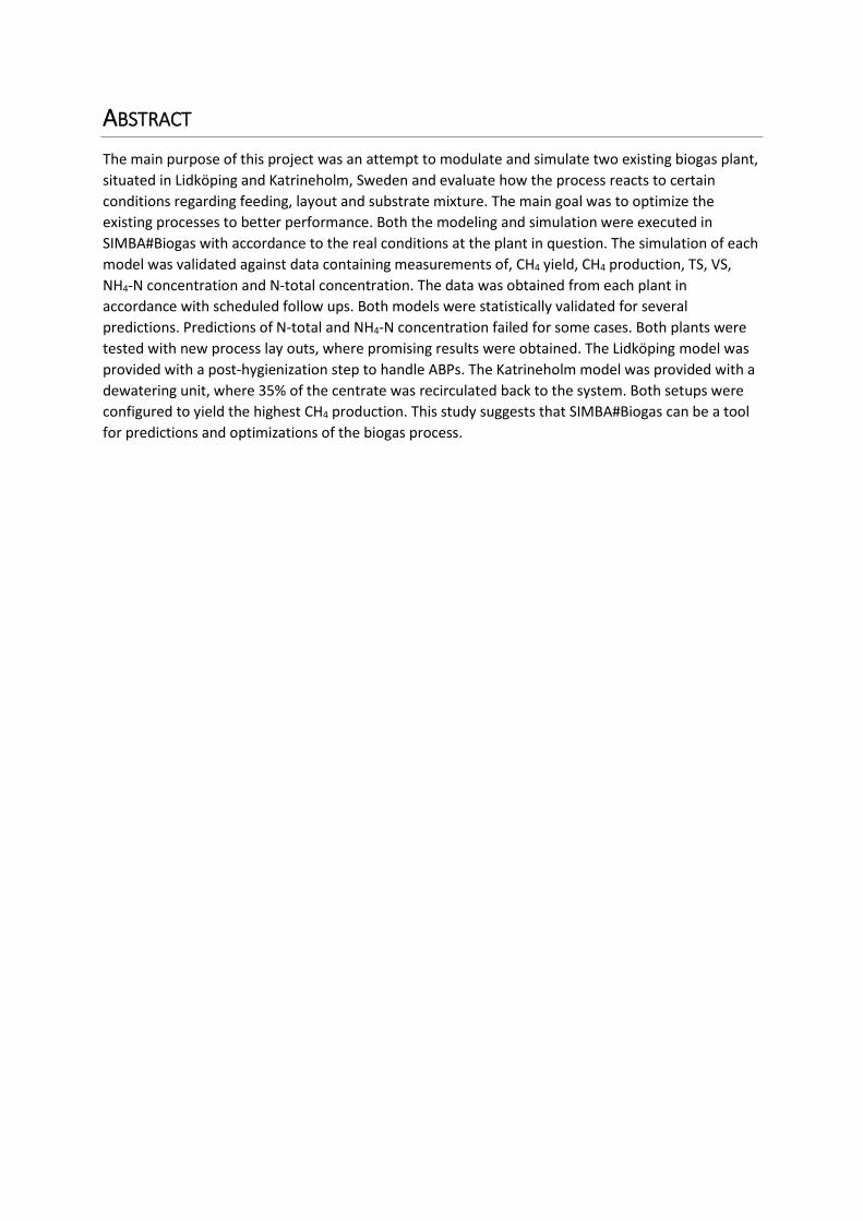
ABSTRACT
The main purpose of this project was an attempt to modulate and simulate two existing biogas plant,
situated in Lidköping and Katrineholm, Sweden and evaluate how the process reacts to certain
conditions regarding feeding, layout and substrate mixture. The main goal was to optimize the
existing processes to better performance. Both the modeling and simulation were executed in
SIMBA#Biogas with accordance to the real conditions at the plant in question. The simulation of each
model was validated against data containing measurements of, CH4 yield, CH4 production, TS, VS,
NH4-N concentration and N-total concentration. The data was obtained from each plant in
accordance with scheduled follow ups. Both models were statistically validated for several
predictions. Predictions of N-total and NH4-N concentration failed for some cases. Both plants were
tested with new process lay outs, where promising results were obtained. The Lidköping model was
provided with a post-hygienization step to handle ABPs. The Katrineholm model was provided with a
dewatering unit, where 35% of the centrate was recirculated back to the system. Both setups were
configured to yield the highest CH4 production. This study suggests that SIMBA#Biogas can be a tool
for predictions and optimizations of the biogas process.
Abbreviations
TS Total solids
TSS Total suspended solids
VS Volatile solids
VSS Volatile suspended solids
ADM1 Anaerobic digestion model number one
ADM1da Anaerobic digestion model number one da
ASM1 Anaerobic sludge model number 1
VFA Volatile fatty acids
BMP Bio methane potential, volume CH4 per mass unit VS
TAC Buffering capacity
CSTR Continuous flow stirred-tank reactor
ABP Animal by-product
SSE Sum of squared errors
SEM Standard error-of-mean
HRT Hydraulic retention time
SRT Solids retention time
GHG Greenhouse gases
Chemical denotations
N Nitrogen
N2 Nitrogen gas
NH3-N Ammonia nitrogen
NH4-N Ammonium nitrogen
N-total Total nitrogen
CO2 Carbon dioxide
CH4 Methane
H2S Hydrogen Sulfide

PREFACE
This thesis concludes my degree in Master of Science in Engineering Biology, with a profile in
Industrial Biotechnology and Production at Linköping University. The work has been conducted at
Gasum AB, Linköping during the spring term of 2017.
Jonas Karlsson, June 2017
LIST OF CONTENT
1. Introduction .................................................................................................................................................... 1
1.1. Purpose of the study ............................................................................................................................. 1
1.2. Expected impact of study ...................................................................................................................... 1
1.3. Objectives of the work ........................................................................................................................... 2
2. Theory and methodology ............................................................................................................................... 3
2.1. Theory .................................................................................................................................................... 3
2.1.1. Biogas ............................................................................................................................................ 3
2.1.2. Anaerobic digestion (AD) .............................................................................................................. 3
2.1.3. Process parameters ...................................................................................................................... 7
2.2. Methodology ......................................................................................................................................... 8
2.2.1. Mathematical modeling ................................................................................................................ 8
2.3. Models ................................................................................................................................................... 8
2.3.1. Anaerobic digestion model number 1 (ADM1) ............................................................................. 8
2.3.2. Converter blocks ......................................................................................................................... 11
3. Material and methods .................................................................................................................................. 14
3.1. Material ............................................................................................................................................... 14
3.1.1. Software ...................................................................................................................................... 14
3.1.2. Biogas plants and measured data ............................................................................................... 14
3.2. Methods .............................................................................................................................................. 17
3.2.1. Analysis of existing biogas plants ................................................................................................ 17
3.2.2. Simulation ................................................................................................................................... 17
3.2.3. Validation .................................................................................................................................... 17
4. Results and discussion .................................................................................................................................. 19
4.1. Lidköping ............................................................................................................................................. 19
4.1.1. Model validation ......................................................................................................................... 21
4.1.2. Test of new substrates and placement of hygienization ............................................................ 24
4.2. Katrineholm ......................................................................................................................................... 29
4.2.1. Model validation ......................................................................................................................... 31
4.2.2. Recirculation of dewatered sludge ............................................................................................. 34
4.3. Summary of results and additional comments .................................................................................... 39
5. Conclusion .................................................................................................................................................... 40
6. Acknowledgement ........................................................................................................................................ 41
7. References .................................................................................................................................................... 42
Appendix A .............................................................................................................................................................. A
Appendix B .............................................................................................................................................................. K
Appendix C .............................................................................................................................................................. O
Appendix D .............................................................................................................................................................. Q
1
1. INTRODUCTION
1.1. PURPOSE OF THE STUDY Gasum AB operates and owns five biogas plants in Sweden, where the production of both biogas and
bio-fertilizer are taking place. Gasum AB has invested in a simulation software for biogas production,
called SIMBA#Biogas. Through simulations of the biogas process, Gasum AB intends to gain a better
project foundation, a more stable production and in the long term gain improved profit.
The main purpose of the project was, with the help of SIMBA#Biogas and along with stored process
data be able to simulate production performance and hence be able to optimize the overall biogas
process in the plants, simultaneously predict the outcome of the process. By using a simulation
software like SIMBA#Biogas, changes in both layout and conditions can be tested. The simulation is
not only helpful when predicting the process, it can also aid to avoid production failures. This, along
with optimization, makes it possible to gain improved profitability (Schön, 2009).
1.2. EXPECTED IMPACT OF STUDY At this point, society is facing issues regarding both the human impact on the environment and the
demand of energy, leading to bio energy resources becoming necessary. The Anaerobic digestion
(AD) process, in which biogas is formed is in this context a clean technology with the capacity to
contribute to rising energy demand (Mata-Alvarez , et al., 2000). Biogas is therefore considered to be
an environmental friendly source of energy. Biogas can be produced from different types of wastes
with high biogas potential, e.g. residues from agricultural activities. (Galí, et al., 2008) in additional,
to the biogas production, says bio-fertilizers can be produced simultaneously, which are of high value
and can be approved as an organic alternative to artificially produced fertilizers. Biogas can be
produced from waste products, which are daily generated in our society (Angelidaki, et al., 2011).
Since energy can be obtained in the shape of biogas, the utilization of wastes as substrates create
values both of the wastes and the society itself. By optimizing the biogas process through modeling
and simulation, more energy can be obtained and the utilization of the added wastes can be
maximized. Hopefully, one will be able to increase the quality of the bio-fertilizers as well. This
altogether have the ability to take our society one step closer to self-sufficiency and at the same time
reduce the emissions of greenhouse gases (GHG).
2
1.3. OBJECTIVES OF THE WORK The main goal of this project was to investigate if SIMBA#Biogas can be used to simulate production
results and be utilized as an optimization tool for the overall biogas process. This includes operation,
control of raw materials and evaluation of changes in the process. This main goal was divided into
five sub goals, which are outlined below.
Goal 1: Was to create a detailed and working simulation model, which reflects the outline and
conditions of the existing plant. The model should be able to describe the processes flow and mixture
of the raw material.
Goal 2: Was to study the mathematical models within the process blocks, which all together form
the overall process. The aim was to secure that correct mathematical model within the process block
was used and performs as expected for the process in question.
Goal 3: Was to evaluate to what degree the simulation corresponds to the measured data from the
plant and find areas where improvements in the model can be done. This included gas yield per
added unit raw material and the effect on the biological process at different production conditions.
Additionally, were simulated results compared with measured data from the plant, i.e. validation of
the model was done.
Goal 4: Was to investigate and evaluate the properties of the different substrates, which were fed to
the plant. This included how these substrates should be described properly in the software. New
substrates were tested and evaluated to see how they affected the process. Additionally, the
placement where the hygienization step yielded the best outcome combined with different types of
substrates was tested.
Goal 5: Was to implement a dewatering unit to the current process system, with the purpose to
minimize the amount of liquid manure. The liquid manure was replaced by a fraction of liquid,
referred as centrate, from the dewatering unit, which was recirculated back to the system. After this
installation, the Total solids (TS) concentration and the concentration of ammonium nitrogen (NH4-N)
in the reactors should be kept below 8% and 5 kg/m3 respectively.
3
2. THEORY AND METHODOLOGY
2.1. THEORY The scientific background behind this project is presented in this section.
2.1.1. Biogas
Biogas is the gas, which is formed when organic material is decomposed by methane producing
microorganisms in anaerobic conditions. Biogas consist mainly of methane (CH4) and carbon dioxide
(CO2) but also nitrogen (N2), hydrogen (H2), hydrogen sulfide (H2S), water (H2O) and other trace
elements from substances, which are depending on the ingoing substrate. The main energy carrier in
this case is the CH4 (Reith, et al., 2003). Both the amount and the composition of the produced biogas
is dependent on the amount, composition and the degradability of the substrate (Wolfsberger,
2008). Biogas is produced through the complex AD process. Many countries around the world are
using biogas as a renewable energy source for heating, electricity and transportation purposes
(Naturvårdsverket, 2012).
2.1.2. Anaerobic digestion (AD)
AD is a process where the production of biogas occurs when complex organic feed stock is degraded
into a range of simpler water-soluble organic compounds, which eventually is converted into a
mixture of gases, among them CH4. The whole process takes place under strictly anaerobic conditions
else, the AD will not function properly. The AD process depends on the coordinated activity of a
complex mixture of microorganisms, which are associated with the transformation of organic
material into mostly CH4 and CO2 (Appels, et al., 2008) , (Kleerebezem, 2014). The AD process is
indeed well suitable for organic waste treatment and biogas is eventually formed meanwhile organic
matter is converted into stable end products (Mudhoo, 2012). The AD follows four different steps,
hydrolysis, acidogenesis, acetogenesis and methaneogenesis. Each of these steps needs its own
group of characterizing microorganisms to function properly (Moestedt, 2015). It is crucial that the
culture of microorganism is in balance. The AD process is commonly used for the treatment of
organic wastes like manure, agriculture wastes, waste water, slaughter house waste and other
industrial organic wastes (Nizami, 2012). The AD process offers the possibility for nutrients recycling,
since digested material can function as bio-fertilizers on agricultural lands, which makes it as a
substitute for artificial fertilizers (Angelidaki, et al., 2011), (Schnürer, et al., 2016). N that is
organically bound in the raw material is mineralized into NH4+ in the AD process, which is readily
accessible to plants when the sludge is used as bio-fertilizers. This is due to the ratio between C and
N decreases when organic matter is released as CH4 and CO2. (Grimsby, et al., 2013)
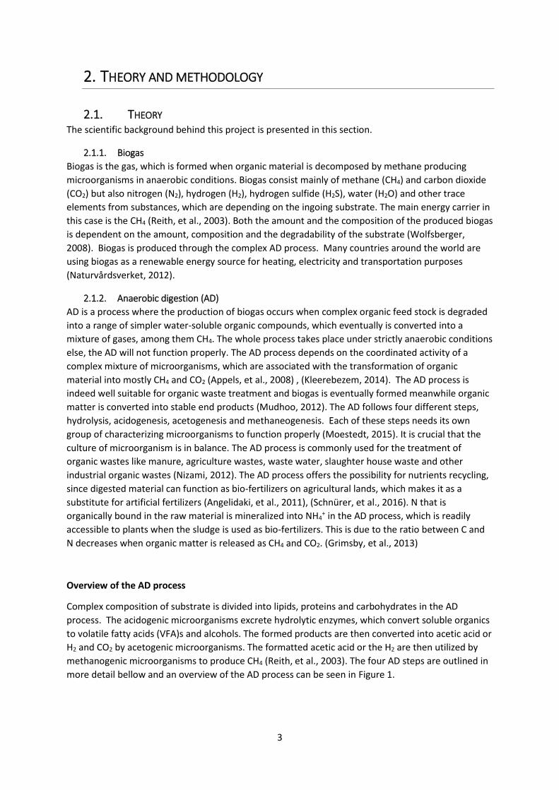
Overview of the AD process
Complex composition of substrate is divided into lipids, proteins and carbohydrates in the AD
process. The acidogenic microorganisms excrete hydrolytic enzymes, which convert soluble organics
to volatile fatty acids (VFA)s and alcohols. The formed products are then converted into acetic acid or
H2 and CO2 by acetogenic microorganisms. The formatted acetic acid or the H2 are then utilized by
methanogenic microorganisms to produce CH4 (Reith, et al., 2003). The four AD steps are outlined in
more detail bellow and an overview of the AD process can be seen in Figure 1.
4
Hydrolysis
The first step in the AD process is hydrolysis, where both insoluble organic material and high
molecular weight compounds are degraded into soluble organic substances.
Examples of such substances that can be degraded into smaller parts in the hydrolysis are nucleic
acids, proteins, lipids, polysaccharides and fatty acids.
The amount of protein in the substrate consists of amino acids, which are linked together with
peptide bonds. These bonds are degraded during the hydrolysis i.e. the bonds are destroyed. The
fraction of carbohydrates in the substrate consists of several types of saccharides and the bond
between the saccharides are broken down by acidogenic and hydrolytic microorganisms during the
hydrolysis.
Lipids are common in the form of triglycerides, which in the hydrolysis are hydrolyzed by lipases. The
rate of the hydrolysis depends less on the substrates’ chemical properties and more on the size of
the particle and environmental conditions such as pH and surface tension (Angelidaki, et al., 2011).
Pre-treatment is necessary if the substrate consist of carbohydrates, which are recalcitrant and hard
to degrade like e.g. cellulose (Lehtomäki, 2016). To make the hydrolyzing step proceeding faster, the
incoming material may be pre-treated. Common pre-treatment methods include mechanical,
thermal, biological or chemical actions (Appels, et al., 2008). The hydrolysis step consumes lot of
time and it is therefore considered to be the rate limiting step in the AD process. (Appels, et al.,
2008) (Reith, et al., 2003)
Acidogensis
During the acidogenesis, soluble organic compounds are converted into VFAs, CO2 and other
compounds (Reith, et al., 2003). Throughout this step, water-soluble chemical substances are turned
into short-chain organic acids i.e. acetic, propionic butyric and pentanoic acid. The remaining
compounds from the hydrolysis can as well be converted into alcohols like methanol and ethanol.
Aldehydes, CO2 and H2 are other compounds, which are formed during this step. (Ziemiński & Frąc,
2012)
The transformation will commonly pass the pathway through acetates, CO2 and H2, whereas other
products from the acidogenesis do not play any significant role. These transformations result in a
directly usage of the new products as substrate and energy source for the methanogens. (Moestedt,
2015)
When the concertation of H2 increases in the system, the microorganisms respond by accumulate
electrons. The accumulation takes form in compounds like lactate, ethanol, propionate, butyrate and
other VFAs. These newly formed compounds cannot directly be utilized by the methanogenic
microorganisms. The newly formed compounds must be converted into H2 by hydrogen producing
microorganisms in a process called acetogenesis. (Ziemiński & Frąc, 2012) The acidogenesis is usually
the fastest step when complex organic matter is converted during anaerobic conditions. If failure in
the process occurs here due to toxicity or inhibitions, the CH4 production will be disturbed and
accumulations of long-and short-chain fatty acids, i.e. VFAs will happen (Schön, 2009).
Acetogenesis
During the Acetogenesis, VFAs are converted into acetate and H2. The previously formed acids are
converted into acetate and H2 by acetate microorganisms. The newly formed acetate and H2 are used
by methanogenetic microorganisms to produce methane. H2 are released during this step, which in

5
turn have toxic effect on the process carrying microorganisms. To establish a properly working
process, a symbiosis is necessary for acetogenic microorganisms with autotrophic methane
microorganisms using hydrogen, which is denoted as syntrophy (Schnürer, et al., 2016). The
acetogenesis is a vital step in the biogas process, since approximately 70 % of the methane arises
when acetates are reduced. Therefore, acetates are considered to be a key intermediary product of
the process of CH4 production. (Ziemiński & Frąc, 2012)
Methanogenesis
The final step in the AD process is called methanogenesis. During this final stage metanogenic
microorganisms are using the products from the previous steps as substrates. Some of these
products are acetate, CO2 and H2, which are converted into CH4 by the methanogenic
microorganisms. The methanogenesis is done by two groups of methanogenic microorganisms: one,
which splits acetate into CH4 and CO2 and another, which uses H2 as donor and CO2 acceptor to
produce CH4 (Appels, et al., 2008). A vast majority of the CH4 arises in the methane digestion process
when acetic acid is converted. The production of CH4 arising from CO2 is only 30% in this step. The
reduction of CO2 is taken care by autotrophic microorganisms and the H2 is consumed during the
process, which in turn contributes to good environmental conditions for the development of acidic
microorganisms. This development give rise to short-chain organic acids in the acidification step. This
in turn leads to declining production of H2 in the acetogenic step. The consequence of this is gas rich
of CO2, since only its trivial part will be transformed into CH4 (Ziemiński & Frąc, 2012). The
methanogenic microorganisms have a reproductive time that lies in a range of 3 to 50 days,
therefore long retention time in the anaerobic reactor is required for proper CH4 production
(Gerardi, 2003).
Figure 1. The figure shows a simplified overview of the AD processes. Proteins, carbohydrates and lipids belongs to the suspended organic matter. Throughout the hydrolysis, these organic matters are degraded into amino acids, sugars and free long chain fatty acids plus glycerol respectively. This is followed by a complex degradation process carried out in three steps i.e. the acidogenesis, acetogenesis and methanogenesis. (de Mes, et al., 2003)
6
AD Inhibitions
The efficiency of the AD process proceeds smoothly if the degradation rates of all stages are equal.
Therefore, inhibition in the first step will affect the rest. This is since the next step will be limited,
which eventually will lead to decreasing CH4 production. If the last step is inhibited, there will be an
accumulation of acids and other compounds in the step before. The inhibition of the last step
happens due to increasing amounts of acids and consequently decreasing pH due to loss of alkalinity.
Process disturbances occurs commonly due to inhibition of methane-forming microorganisms in the
methanogensis step. As previously mentioned, the AD process contains different groups of
microorganisms, which work in sequence and each group forms and provides substrates for another
group (Schnürer & Jarvis, 2009). Hence, each group of microorganisms is linked to another in
chainlike manner, where the weakest links being the production of acetate and methane (Gerardi,
2003). Below, three common inhibition parameters are presented.
pH
The optimum pH level differs between the microbial groups but overall, the formation of CH4
occurs within a pH interval of 6.5 to 8.5. However, the methane producing microorganisms
are highly sensitive to pH and thrives best when the pH lies between 7.0 and 8.0 (Weiland,
2010), (Kumar Khanal & Li, 2016). The fermentative microorganisms in the acidogensis and
acetogensis are less sensitive and can function in environments with pH values between 4
and 8.5. If the pH value decreases, and reaches a low level, the main products are acetic and
butyric acids, whereas at pH values above 8, acetic and propionic acid are being produce
(Appels, et al., 2008). Inhibition of the AD process occurs when the pH values drop below 6.0
or exceeds 8.0 (Weiland, 2010).
The measurement of the pH value is relatively easy to execute, but due to the complexity of
the AD process, interpretation of a change in the value is more difficult (Pind, 2003).
Ammonia (NH3)
Ammonia is formed when nitrogenous matter is biological degraded, mostly in the form of
proteins and urea (Chen, 2008). There are a few inhibitions related to the presence of NH3.
Ammonia NH3 is an inhibitor compound, which can pass over the cell membrane, due to its
hydrophobic properties. When inside the cell, it affects and lowers the internal cellular pH,
leading to a shift towards NH4 +. This results in changes, affecting both the cell pH and the
trans-membrane potential (Moestedt, 2015). The methanogenic microorganisms are least
tolerant to ammonia-related inhibitions and their growth are likely to cease during high NH3
conditions (Chen, 2008).
Volatile fatty acids (VFA)
The concentration of VFAs in the system have a certain impact on the pH level. If there is a
high concentration of VFAs, the pH level will decrease and a chain reaction is started. It can
be explained by the microorganisms’ efficiency decreases, leading to accumulation of VFAs,
which in turn leads to even lower pH. VFAs are key intermediaries and are produced by
acidogenic microorganisms together with CO2, H2S and other by-products. (Pind, 2003) All
these by-products are affecting the system in some way and thereby contribute to inhibitions
(Appels, et al., 2008). Accumulation of VFAs might be related to substrate overload or
inhibitions in the methanogenic step of the AD process (Schnürer & Jarvis, 2009).

7
2.1.3. Process parameters
The process is affected by several parameters and some of them are presented below.
Temperature
The biogas process can be conducted at either psychrophilic (10-20 °C), mesophilic (20-40 °C)
or thermophilic (50-60 °C) conditions (de Mes, et al., 2003).
Temperature has a certain impact on the biochemical reaction in five main ways (Batstone,
et al., 2002):
- Elevated temperature will lead to faster reaction rates
- Lowered reaction rate with elevating temperature above optimum. (Over 40 °C for
mesophilic and over 65 °C for thermophilic microorganisms)
- Increased turnover and maintenance energy with increased temperature, resulting in
lowered yield.
- Due to changes in thermodynamic yields and microbial population there will be shifts in
yield and reaction pathway.
- Increased lysis and maintenance, leading to increased death rate.
Even small temperature changes can affect the degradation rate and hence the CH4
production (Chen, 2008). Increased temperature can lead to increasing concentration of free
NH3, resulting in inhibition of the AD process (Appels, et al., 2008).
Total and volatile solids (TS and VS)
Two typical control parameters in biological treatment processes are TS and VS.
TS is defined as the mass percentage, which is left after the substrate has been dried at 105
°C. The VS is set in relation to TS and is defined as the mass percentage of material, which is
left after combustion at 550-600 °C. (Satpathy, et al., 2013) VS is the accessible amount of
organic material, which also is the amount of material that theoretically can be turned into
biogas (Angelidaki & Ellegaard, 2003). However, there are materials, such as wood, which
have high organic content but is directly unsuitable for biogas production through the AD
process.
Hydraulic and solid retention time (HRT and SRT)
Retention time denotes the time it takes to exchange the entire material volume in the
reactor. HRT is the average time the sludge is present in the reactor and it is defined as the
relation between the working volume and the daily input (Appels, et al., 2008). SRT is the
average time the solids stays in the reactor. HRT and SRT are in many cases equally long, but
in cases with recirculation where a part of the sludge is recirculated back to the reactor, the
SRT is longer than the HRT. The HRT is commonly 10 to 25 days long but it can also be longer.
(Schnürer & Jarvis, 2009) Short HRT increases the risk for accumulations of VFAs within the
processes and thereby the risk for inhibitions and insufficient degradation rises (Appels, et
al., 2008).
Chemical oxygen demand (COD)
COD is a measurable parameter that states the total chemically oxidizable material in a
sample, which in turn indicates the energy content of the feedstock. The COD represents the
maximum chemical energy, which is present in the feedstock. This stored chemical energy is
converted by microbes to CH4. This is as well the maximum energy, which could be recovered
as biogas, however losses for the energy demand of the microbes themselves must be
8
subtracted and the same applies for material that is not degradable by anaerobic
microorganism, like ligno cellosic compounds. (Wellinger, et al., 2013)
2.2. METHODOLOGY
2.2.1. Mathematical modeling This project was based on the mathematics in the widely used Anaerobic digestion model number 1
(ADM1) (Batstone, et al., 2002). Mathematical modeling is a tool, which makes it possible to
investigate the static and dynamic behaviors of a system. This can in best cases be done without
doing practical experiments. With help from obtained measured data, the rest can be simulated by a
model after proper calibration and validation. (Schön, 2009)
2.3. MODELS In this section is the model used in this project is presented.
2.3.1. Anaerobic digestion model number 1 (ADM1)
The ADM1 is a structured and COD based model, which include all the fundamental reaction steps in
the previous presented AD process (Lübken, et al., 2007), (Blumensaat & Keller, 2004). The strength
of this model lays in its consideration of separating biomass into different fractions and their decay,
apart from including the four main phases of anaerobic degradation and dividing them into 31
processes and 33 group fractions. Additionally, the model considers a composite fraction (XC), which
corresponds to a complex substrate and is treated homogenously by the model. The XC is degraded
into four different fractions during the disintegration phase. These fractions are carbohydrates (XCh),
proteins (XPr), lipids (Xli) and inert (XI). (Batstone, et al., 2002) Thanks to the model’s ability to
describe the production rate of biogas, the ADM1 is frequently used as an anaerobic degradation
model for different substrates (Biernacki, et al., 2013).
The original ADM1 contains 39 different states, 24 soluble components (Si), 3 gaseous components
(Sgasi), 5 particulate composites (Xi) where i stands for the component and 7 microbial groups (Xj),
where j stands for the degrading component. 10 of 24 soluble components concern the acid-base
equilibrium. The majority of them are expressed either in terms of COD or kmole nitrogen (N) or
carbon (C) per m3.
The reactions, which takes place within an anaerobic digester are complex with a number of
sequential and parallel stages. These reactions may be divided into biochemical and physio-chemical
reactions.
Biochemical reactions and processes
These are reactions, which are commonly catalyzed by intra or extracellular enzymes and act
on the pool of accessible organic material. Disintegration of compounds into particulate
elements and the subsequent enzymatic hydrolysis of these to their soluble monomers are
extracellular. Soluble materials are degraded with facilitation of intracellular organisms,
leading to growth in biomass and subsequent decay. The AD process steps, acidogenesis,
acetogenesis and hydrolysis, which were previously presented in section 2.1.2, have several
parallel reactions.
9
Physio-chemical reactions and processes
These reactions are not biologically mediated and include association/dissociation of ions as
well gas-liquid transfer. Precipitate is also counted to the physio-chemical reaction, but it is
however not included in the ADM1.
The ADM1 has since its release been utilized as the foundation for several studies and different
modifications have been applied to modify it to fit specific processes. The ADM1 is however not
suitable for either plug-flow or solid-state digesters, since the model assumes ideal mixing and
homogeneous reactor content (Kumar Khanal & Li, 2016).
The ADM1 and its variables and parameters are presented in appendix B. For complete information
about the ADM1, the reader is referred to (Batstone, et al., 2002).
Inhibition
Since the inhibitions within the AD process are varied and extensive, the forms of them are
expressed as Equation 1 in ADM1.
Equation 1. 𝜌𝒋 =𝑘𝒎𝑆
𝐾𝑠+𝑆𝑋 ∗ 𝐼1 ∗ 𝐼2 … 𝐼𝑛
The first part of Equation 1 represents the uninhibited Monod-type uptake and I1..n = f(SI,1..n) are the
inhibition functions presented in Table A and Table B in appendix B. In cases when this equation is
not applicable, due to the inhibition function is integral in the uptake equation, the full uptake
equations are shown in Table C in appendix B. (Batstone, et al., 2002)
ADM1da
The original ADM1 is indeed a powerful model, however it has some drawbacks when it comes to
modeling the complexity of the biogas process. The ADM1 offers only one composite fraction (XC),
which is degraded into previously presented fractions XCH, XPr, Xli and XI. Since a wide range of
different substrates are commonly utilized at a biogas plants and due to high variety in amount and
proportion of carbohydrates, proteins and lipids of different particulate organic matter, this original
division of the XC is insufficient to describe the biogas processes to the right extent. To come around
this problem, several approaches have been proposed. A division of the particulate sugars (XCH) into
rapid and slow hydrolysable portion was proposed by (Wolfsberger, 2008). Additionally, changes
were implemented in the model, where the composite fraction (XC) was split into a rapid and slow
disintegrable portions, whereas both fractions are still disintegrated into fixed proportions (Rojas, et
al., 2011).
Focusing on agricultural biogas plants, the model structure was implemented with an intervention,
according to (Schlattmann, 2011). This made it possible for the model to handle fractions that are the
output of the Weender animal feed analysis presented in (Henneberg & Strohmann, 1864).
The new features regarding the organic particulate material lead to the introduction of further
degradable fractions. Thereby, the biogas production and its degradation processes can be better
described. On the other hand, there is still some challenges regarding the balance of inorganic
nitrogen, which has great impact on the buffer system. The reason for this is related to the formation
of biologically inert substances (XI) by disintegration of different particulates including biomass,
meaning the biological inert substances composition and its N content is deepening on the type and
mixture of organic particulates. To be able to represent the products that arises from the biomass
decay, the fraction (XP) was introduced and contributes with different N content as XI, which in turn
10
refines the overall N balance of the plant. This coupled the anaerobic sludge model number 1 (ASM1)
with the ADM1 (Wett, et al., 2006).
Through implementation of presented changes in the model, ADM1da was created. ADM1da
differentiates disintegrable organic materials into a slow (XPS) and a fast disintegrable (XPF) fraction
and then expresses all dissolved and particulate organic materials by the appropriated sub-fractions
(CH, PR, LI, SU, AA, FA). (ifak e.V, 2016) The changes in ADM1 compared to ADM1da are presented in
Table D in appendix B.
Reactor model
The implementation of ADM1 into reactor model was based on a continuous flow stirred-tank
reactor (CSTR) approach. The model combines four different mathematical models for the
description of
i. The bio-chemical processes in the sludge phase.
ii. The composition of the gas phase.
iii. The mass transfer between sludge and gas phase
iv. The derivation of process describing parameter e.g. VFA or buffering capacity (TAC).
This combination is necessary due to the impact on the acid-base system from the interrelation
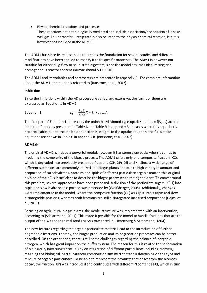
between sludge phase and gas phase. Figure 2 describes the combination of these four models in the
reactor. (ifak e.V, 2016), (Kumar Khanal & Li, 2016).
Figure 2. The figure show the modeling approach for the reactor (ifak e.V, 2016). q = flow [m3/day], V = volume [m3], Sstream,I
= concentration of soluble components [kgCOD/ m3] Xstreams, I = concentration of particulate components [kgCOD/ m3]. The i is the component index. (Batstone, et al., 2002)
Liquid phase
The mass balance for each state component can be written as Equation 2.
Equation 2. 𝑑𝑉𝑆𝑙𝑖𝑞,𝑖
𝑑𝑡= 𝑞𝑖𝑛𝑆𝑖𝑛,𝑖 − 𝑞𝑜𝑢𝑡𝑆𝑙𝑖𝑞,𝑖 + 𝑉 ∑ 𝜌𝑗𝑣𝑖,𝑗𝑗=1−19
Where the term ∑ 𝜌𝑗𝑣𝑖,𝑗𝑗=1−19 is the summation of the specific kinetic rates for process j times 𝑣𝑖,𝑗,
which is the rate coefficients component i for processes j. If one assume a constant volume i.e. 𝑞 =
𝑞𝑖𝑛 = 𝑞𝑜𝑢𝑡), the expression can be written as Equation 3.
Equation 3. 𝑑𝑆𝑙𝑖𝑞,𝑖
𝑑𝑡=
𝑞𝑆𝑖𝑛,𝑖
𝑉𝑙𝑖𝑞−
𝑞𝑆𝑙𝑖𝑞,𝑖
𝑉𝑙𝑖𝑞+ ∑ 𝜌𝑗𝑣𝑖,𝑗𝑗=1−19
11
When the volume is assumed to be fluctuating with time, the expression can be written as Equation
4.
Equation 4. 𝑑𝑋𝑙𝑖𝑞,𝑖
𝑑𝑡=
𝑞𝑋𝑖𝑛,𝑖
𝑉𝑙𝑖𝑞−
𝑋𝑙𝑖𝑞,𝑖
𝑡𝑟𝑒𝑠,𝑋+𝑉𝑙𝑖𝑞
𝑞
+ ∑ 𝜌𝑗𝑣𝑖,𝑗𝑗=1−19
Where 𝑡𝑟𝑒𝑠,𝑋 is the residence time of solid components beyond HRT. If 𝑡𝑟𝑒𝑠,𝑋 = 0 the overall SRT
is 𝑉𝑙𝑖𝑞
𝑞.
Gas phase
The equations for the gas phase rate are very similar to the liquid phase equations. The dynamic
state component can be expressed in pressure (bar) or in concentration (M or kgCOD m-1). The
pressure is calculated with the ideal gas law 𝑝 = 𝑆𝑅𝑇, where 𝑆 is the concentration in M. The
expression for a gas phase with constant gas volume can be written as Equation 5.
Equation 5. 𝑑𝑆𝑔𝑎𝑠,𝑖
𝑑𝑡= −
𝑆𝑔𝑎𝑠,𝑖𝑞𝑔𝑎𝑠
𝑉𝑔𝑎𝑠+ 𝜌𝑇,𝑖
𝑉𝑙𝑖𝑞
𝑉𝑔𝑎𝑠
The head space of the reactor can be assumed to be water vapor saturated and is described by
Equation 6.
Equation 6. 𝑝𝑔𝑎𝑠,𝐻2𝑂 = 0,0313𝑒(5290(
1
298−
1
𝑇))
Where the temperature is denoted as T in K. The gas flow is calculated per Equation 7.
Equation 7. 𝑞𝑔𝑎𝑠 =𝑅𝑇
𝑃𝑔𝑎𝑠−𝑝𝑔𝑎𝑠,𝐻2𝑂𝑉𝑙𝑖𝑞(
𝜌𝑇,𝐻2
16+
𝜌𝑇,𝐶𝐻4
64+ 𝜌𝑇,𝐶𝑂2
)
Where 𝑃𝑔𝑎𝑠 is the total pressure in the head space of the reactor.
For more detailed information about the CSTR implementation, the reader is referred to (Batstone,
et al., 2002).
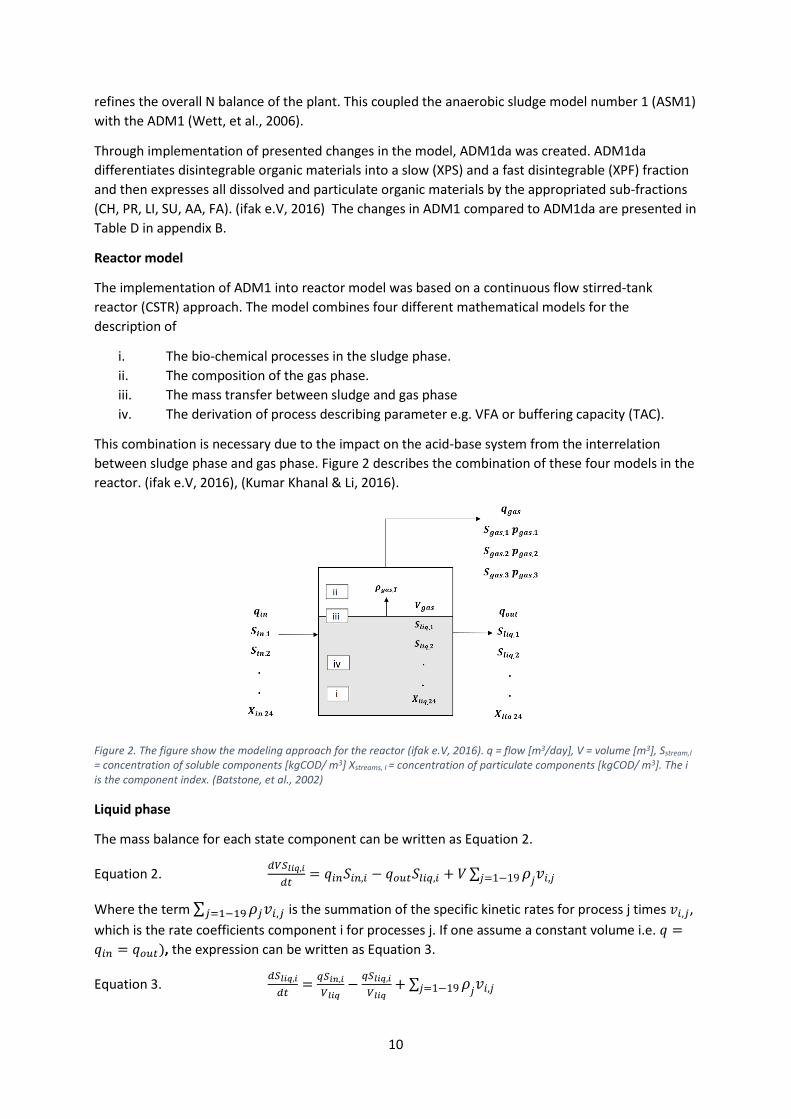
2.3.2. Converter blocks
One important feature in SIMBA#Biogas is the converter blocks, which specifies the character of the
ingoing substrates. The different substrates must be specified and their values must as well be
translated into information, which the ADM1da can utilize. In Figure 3, one can see a simplified
overview of how the converter block functions.
Figure 3. Converter block for the ingoing substrate
12
The input consists of total suspended solids (TSS), volatile suspended solids (VSS) and flow. For some
substrates, like manures and silages, the value for NH4-N must be specified. The parameter values
are specified per the user’s choice. Inside the block, different variables are calculated based on the
input and parameter values. The output values are then used to calculate different reactions in the
ADM1da. Explanations for each input, parameter and output values are outlined in Table 1, Table 2
and Table 3 respectively.
Table 1. The table show all ingoing data to the converter block.
Input
Id Description Unit
TSS Total suspended solids kg/m3
VSS Volatile suspended solids kg/m3
NH4FM Ammonium-nitrogen kg N/m3
FM Fresh mass flow Ton/day
Table 2. The table show the parameter values, which are set by the user.
Parameters
Id Description Group Unit
fOTSrf Degradable fraction of crude fiber (XF) Degradability
fsOTS Slowly disintegrable fraction of VSS Degradability
ffOTS Fast disintegrable fraction of VSS Degradability
aXI Particulate inert fraction of COD Degradability kg COD/kg COD
aSI Soluble inert fraction of COD Degradability kg COD/kg COD
fRF Crude fiber fraction (XF) of TSS Weender Parameter kg TSS/kg TSS
fRP Crude protein fraction (XP) of TSS Weender Parameter kg TSS/kg TSS
fRFe Crude lipid fraction (XL) of TSS Weender Parameter kg TSS/kg TSS
Temp Temperature Buffer system °C
pH pH-Value Buffer system
KS43 Acid capacity (pH 4.3) Buffer system mol/m3
FFS Volatile fatty acids Buffer system kg AC/m3
Since the disintegration step in ADM1da is divided into the two fractions, slowly and fast
disintegrable fraction of VS, the user must specify these fractions. Unfortunately, there is a lack of
data for these fractions, which means that the user needs to do arbitrary estimations here (Schön,
2009). For most cases, the soluble inert fraction of COD lies around 0.1. The particulate inert fraction
of COD was roughly estimated accordingly to Equation 8.
Equation 8. 𝑎𝑋𝐼 = 𝑓𝑂𝑇𝑆𝑟𝑓 − 𝑎𝑆𝐼
The convert block specifies the properties of the substrate based on Weender parameters, which
specifies the crude nutrients i.e. protein, lipids and fibers for the substrate in question.
Crude protein is calculated with Equation 9. Here are non-protein nitrogen compounds like NH3 and
urea included (Wiley-VCH, 2016). Free NH4+ is however not included.
Equation 9. 𝑋𝑃 = 𝑁 ∗ 6,25
Crude lipids include lipids and lipid-similar compounds. This includes waxes, phospholipids
glycolipids, etc (Wiley-VCH, 2016).
13
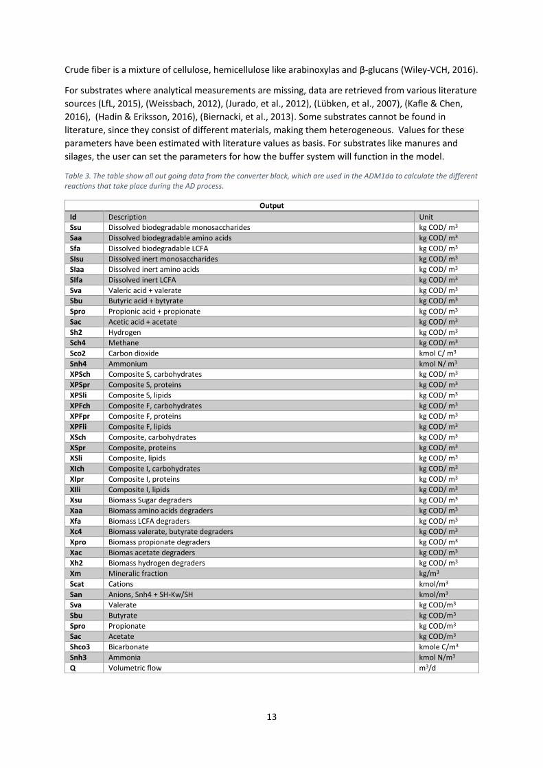
Crude fiber is a mixture of cellulose, hemicellulose like arabinoxylas and β-glucans (Wiley-VCH, 2016).
For substrates where analytical measurements are missing, data are retrieved from various literature
sources (LfL, 2015), (Weissbach, 2012), (Jurado, et al., 2012), (Lübken, et al., 2007), (Kafle & Chen,
2016), (Hadin & Eriksson, 2016), (Biernacki, et al., 2013). Some substrates cannot be found in
literature, since they consist of different materials, making them heterogeneous. Values for these
parameters have been estimated with literature values as basis. For substrates like manures and
silages, the user can set the parameters for how the buffer system will function in the model.
Table 3. The table show all out going data from the converter block, which are used in the ADM1da to calculate the different reactions that take place during the AD process.
Output
Id Description Unit
Ssu Dissolved biodegradable monosaccharides kg COD/ m3
Saa Dissolved biodegradable amino acids kg COD/ m3
Sfa Dissolved biodegradable LCFA kg COD/ m3
SIsu Dissolved inert monosaccharides kg COD/ m3
SIaa Dissolved inert amino acids kg COD/ m3
SIfa Dissolved inert LCFA kg COD/ m3
Sva Valeric acid + valerate kg COD/ m3
Sbu Butyric acid + bytyrate kg COD/ m3
Spro Propionic acid + propionate kg COD/ m3
Sac Acetic acid + acetate kg COD/ m3
Sh2 Hydrogen kg COD/ m3
Sch4 Methane kg COD/ m3
Sco2 Carbon dioxide kmol C/ m3
Snh4 Ammonium kmol N/ m3
XPSch Composite S, carbohydrates kg COD/ m3
XPSpr Composite S, proteins kg COD/ m3
XPSli Composite S, lipids kg COD/ m3
XPFch Composite F, carbohydrates kg COD/ m3
XPFpr Composite F, proteins kg COD/ m3
XPFli Composite F, lipids kg COD/ m3
XSch Composite, carbohydrates kg COD/ m3
XSpr Composite, proteins kg COD/ m3
XSli Composite, lipids kg COD/ m3
XIch Composite I, carbohydrates kg COD/ m3
XIpr Composite I, proteins kg COD/ m3
XIli Composite I, lipids kg COD/ m3
Xsu Biomass Sugar degraders kg COD/ m3
Xaa Biomass amino acids degraders kg COD/ m3
Xfa Biomass LCFA degraders kg COD/ m3
Xc4 Biomass valerate, butyrate degraders kg COD/ m3
Xpro Biomass propionate degraders kg COD/ m3
Xac Biomas acetate degraders kg COD/ m3
Xh2 Biomass hydrogen degraders kg COD/ m3
Xm Mineralic fraction kg/m3
Scat Cations kmol/m3
San Anions, Snh4 + SH-Kw/SH kmol/m3
Sva Valerate kg COD/m3
Sbu Butyrate kg COD/m3
Spro Propionate kg COD/m3
Sac Acetate kg COD/m3
Shco3 Bicarbonate kmole C/m3
Snh3 Ammonia kmol N/m3
Q Volumetric flow m3/d
14
3. MATERIAL AND METHODS
3.1. MATERIAL In this section, materials used during this project are presented.
3.1.1. Software
The biogas plants were modeled and simulated in the independent simulation software
SIMBA#Biogas created by the company ifak technology (Department of water and energy). The
software is versatile and can perform dynamic simulation of biogas plants which is based on the wet
digestion principle. The simulations in SIMBA#Biogas is based on mathematical modelling and can
serve as a valuable tool in design, analysis and optimizations of processes that occurs at a biogas
plant (Schön, 2009).
The library in SIMBA#Biogas offers a row of components, which are needed to make a proper
analysis of wet digestion plants. The software is based on ADM1, created by the International Water
Association (Batstone, et al., 2002). The software can be used to design and optimize a plant’s layout,
processes and control concepts. (ifak , 2016) The software has a drag and drop interface with
different model blocks. Each model block symbolizes a certain process unit in the biogas plant, e.g. a
reactor or a gas storage. Other model blocks represent storage of material, sludge or gas flow
routing. The model blocks can then easily be connected with lines, which represent material or
sludge flow vectors. The model blocks are all found in the included library. (Fronk, et al., 2014) Two
example of how a model can look like are illustrated in Figure 6 and Figure 11.
Key functions in SIMBA#Biogas
Pre-configured input models for a number of agricultural waste sources
Bio kinetics based on ADM1
High range of support for different process control concepts
Predictions of various types of parameters
3.1.2. Biogas plants and measured data
In this section, information about the modeled biogas plants will be presented.
Lidköping
The biogas plant in Lidköping was ready for production in January 2011. During 2016, the facility
produced 6 million Nm3 bio methane and consumed 60 000 ton substrate. In addition to the
production of CH4, it generates 50 000 ton of bio-fertilizer per year. The substrate used is a mixture
between different food and agricultural waste products from the regional area (Gasum AB, 2017).
The plant has four reactors where the digestion is done in two steps. The two main and post reactors
have a volume of 4200 m3 and 2600 m3 respectively. The plant has a 5300 m3 covered bio-fertilizer
storage tank, functioning as a buffer storage with fluctuating volume. The bio-fertilizer tank is
connected to the raw-gas system. The temperature in the main and post reactor are approximately
39˚C and 38˚C respectively, meanwhile the temperature in the uninsulated fertilizer tank fluctuates
depending on the outside temperature. The main digestors have solid roofs meanwhile the post
digeters have dubbel membrane roofs, which function can be compared to a lung. The side mounted
mixtures in the post reactors are lubricated with water, this is also the case for the substrate tanks
contaning starch residues. The upgrade is done with water scrub technology and the upgraded gas is

15
delivered to the customer on the other side of the fence, where it is liquefied. The rest is compressed
to mobile gas storages. An overview of the plant can be seen in Figure 4.
Figure 4. Overview of the plant in Lidköping (Gasum AB, 2017). 1) solid substrate reception, 2) storage tank, 3) grain silos, 4) main reactors, 5) post reactor, 6) bio-fertilizer tank, 7) gas upgrading unit, 8) flare, 9) office and 10) costumer. (Gasum AB, 2017)
The feed stock in Lidköping consists of different agricultural rest products. The average amount for
2016 of each substrate and some basic properties can be seen in Table 4.
Table 4. The table shows the average amount of ingoing feed during 2016. TS, VS, total nitrogen (N-total) concentration and estimated digester degradability are also presented in the table.
Substrate Average feed in [ton/day]
TS [%]
VS [% of TS]
N-total [kg/ton] Estimated Degradability
[%]
Starch residues 176 7 97 2.8 95
Solid materials of agricultural origin
39 80-90 90-97 11.4-34.1 65-90
Silages 7 32-36 90 3.8-5 60
Katrineholm
The biogas plant situated in Katrineholm is a so-called co-digestion plant, which means that different
types of substrates are mixed and degraded together e.g. grains and animal by-products (ABP)s. The
biogas production started December 2010. The plant produces 3 million Nm3 bio methane, 60 000-
ton bio-fertilizer and consumes 70 000 ton substrate per year. (Gasum AB, 2017) The biogas plant
consist of two parallel digesters, each with a volume of 4400 m3. The plant in Katrineholm is
equipped with a hygienization step, heated to 70˚C. The hygienization is done by a series of heat
exchangers with water-sludge transfer. The ingoing sludge into the heat exchanger is heated by
water used for cooling down the sludge completed the hygienization step. A special heater is used to
reach above 70°C. The hygienization step is necessary, since the plant uses ABPs as substrate. The gas
upgrading is done with water scrubber technology. The upgraded gas is then compressed into mobile
gas storages for further distribution by the customer to the surroundings. (Gasum AB, 2017) The
temperature in both reactors hold approximately 38˚C.
16
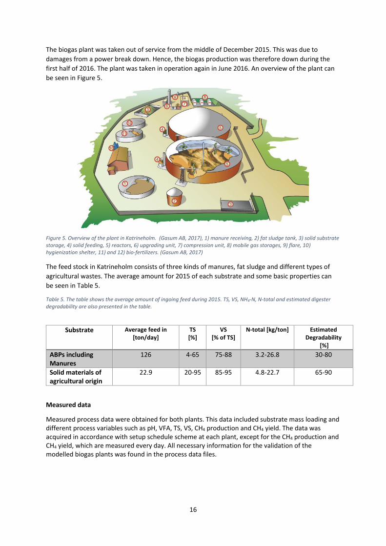
The biogas plant was taken out of service from the middle of December 2015. This was due to
damages from a power break down. Hence, the biogas production was therefore down during the
first half of 2016. The plant was taken in operation again in June 2016. An overview of the plant can
be seen in Figure 5.
Figure 5. Overview of the plant in Katrineholm. (Gasum AB, 2017), 1) manure receiving, 2) fat sludge tank, 3) solid substrate storage, 4) solid feeding, 5) reactors, 6) upgrading unit, 7) compression unit, 8) mobile gas storages, 9) flare, 10) hygienization shelter, 11) and 12) bio-fertilizers. (Gasum AB, 2017)
The feed stock in Katrineholm consists of three kinds of manures, fat sludge and different types of
agricultural wastes. The average amount for 2015 of each substrate and some basic properties can
be seen in Table 5.
Table 5. The table shows the average amount of ingoing feed during 2015. TS, VS, NH4-N, N-total and estimated digester degradability are also presented in the table.
Substrate Average feed in [ton/day]
TS [%]
VS [% of TS]
N-total [kg/ton] Estimated Degradability
[%]
ABPs including Manures
126 4-65 75-88 3.2-26.8 30-80
Solid materials of agricultural origin
22.9 20-95 85-95 4.8-22.7 65-90
Measured data
Measured process data were obtained for both plants. This data included substrate mass loading and different process variables such as pH, VFA, TS, VS, CH4 production and CH4 yield. The data was acquired in accordance with setup schedule scheme at each plant, except for the CH4 production and CH4 yield, which are measured every day. All necessary information for the validation of the modelled biogas plants was found in the process data files.
17
3.2. METHODS
3.2.1. Analysis of existing biogas plants
The modeling was based on the two different biogas plants, presented in section 3.1.2. The chosen
plants were situated in Lidköping and Katrineholm, Sweden. The plant differs in size, lay out, total
CH4 production and mixture of substrate. To gain a better understanding of the plants and how they
function in reality, a study visit was conducted to each plant. The modeling was first started after the
study visits.
3.2.2. Simulation
The simulation of the biogas process was executed in SIMBA#Biogas v 2.043. The simulations were
done with the modified version of ADM1, called ADM1da presented in section 2.3. Two types of
simulations were done, one where the average value for the ingoing feed stock was used to create a
steady state condition and another that used the first simulation as initial phase. The creation of the
steady state was done by letting the model use the average amount of loaded feed stock during a
simulation time of 500 days. In the second simulation, the model used the raw alternating feeding
data for the ingoing feedstock expressed in tons per day. The length of the simulation was depending
on the numbers of days data were available.
In the cases where the original models were modified to test new conditions, layouts and substrates,
only one simulation were executed i.e. no steady state was used.
3.2.3. Validation
The validation of the models were done against measured data from each plant. The models were
matched against the yield and production of CH4, TS, VS, concentration of NH4-N and N-total.
Cost function
A cost function was used to determine the error between simulated model data y(i) and measured
data f(x(i)) (Arnell, 2016). The differences between simulated and measured data is referred as
residuals. In the case when the calculated residuals are large, particularly when they are large
compared to the uncertainty in the data, the model will not be able to give an accurate explanation
for the data. The size of the residuals is tested in a chi-square test, which is presented in the next
section. In the case where most of the residuals are alike their neighbors e.g. if the simulation lies on
the same side of the experimental data for the greater part of the data set, the model cannot explain
the data accurately. (Cedersund & Roll, 2009) The cost function was based on the summation of sum
of squared errors (SSE) weighted with standard error-of-mean (SEM). The SEM was estimated as the
standard deviation for the whole measured data set. The setup for the SSE and cost function can be
seen in Equation 10 and 11 respectively. (Arnell, 2016), (Cedersund & Roll, 2009)
Equation 10. 𝑆𝑆𝐸 = ∑ (𝑦(𝑖) − 𝑓(𝑥(𝑖)))2𝑛𝑖=1
Equation 11. 𝑉 =𝑆𝑆𝐸
𝑆𝐸𝑀2
18
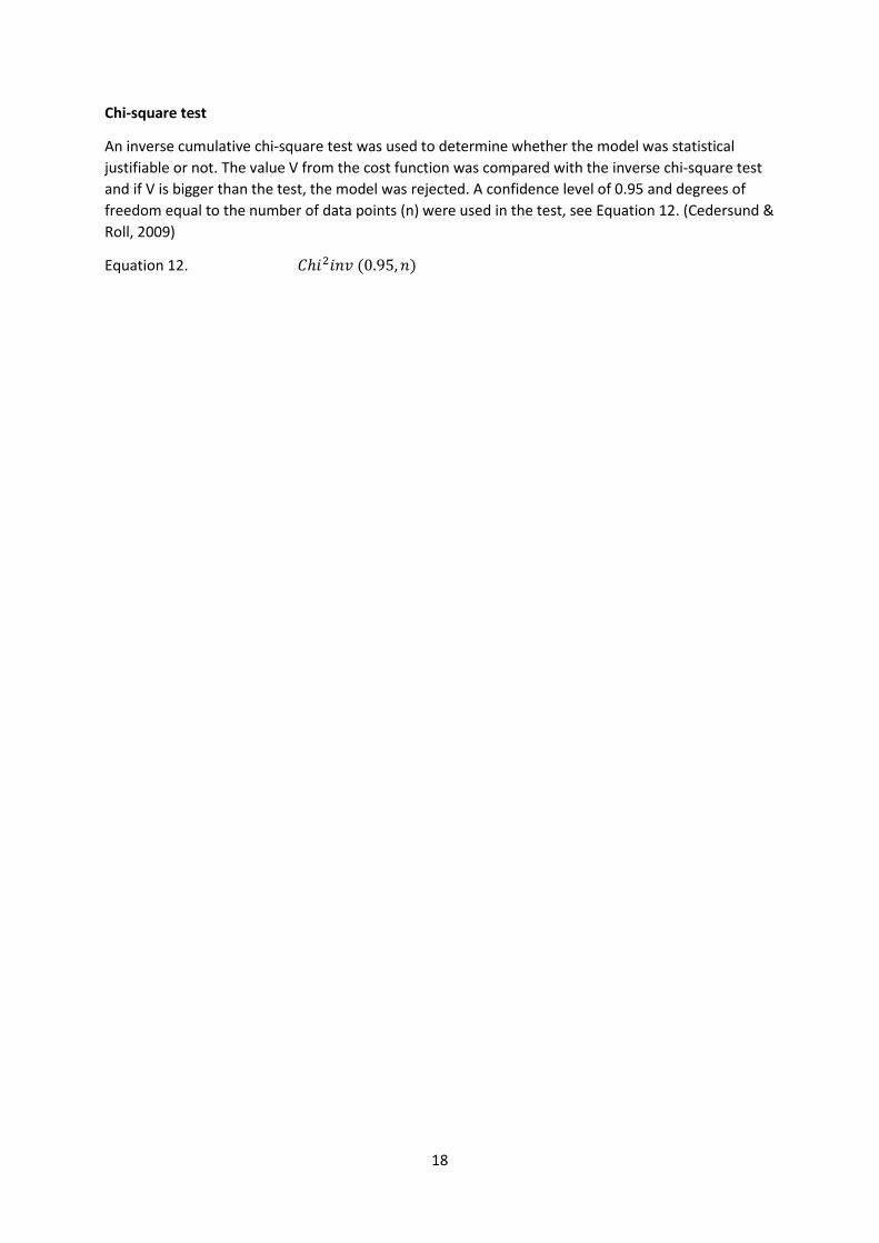
Chi-square test
An inverse cumulative chi-square test was used to determine whether the model was statistical
justifiable or not. The value V from the cost function was compared with the inverse chi-square test
and if V is bigger than the test, the model was rejected. A confidence level of 0.95 and degrees of
freedom equal to the number of data points (n) were used in the test, see Equation 12. (Cedersund &
Roll, 2009)
Equation 12. 𝐶ℎ𝑖2𝑖𝑛𝑣 (0.95, 𝑛)
19
4. RESULTS AND DISCUSSION
In this section, the results from the simulation of the modeled plants will be presented. Explanations
of measurements and denotations are presented in Table 6 and Table 7.
Table 6. The table presents the explanations for the five measurements, which are applied in the simulations.
Measurement Explanation
CH4 yield The amount of acquired 97% methane per ton added volatile solids
CH4 production The amount of acquired vehicle gas i.e. gas upgrade to 97% methane content
TS The number of total solids in the reactor
VS The number of volatile solids in the reactor
NH4-N concentration The concentration of ammonium nitrogen in the reactor
N-total concentration The concentration of total nitrogen
Table 7. The table presents the explanations for the five denotations in the analysis of the result.
Denotation Explanation
Mean The average value for a specific data set
n The number of used data points
V The value given by the cost function
Chi2 The value given by the inverse Chi-squared test
d The differences between simulated and measured values
4.1. LIDKÖPING The model of the plant in Lidköping consist of nine different substrates, which all are individully
specified in converter blocks. To match the feed pattern to reality, the amount of each substrate are
retrived from a spread sheet, where each colum contains the amount of substrate in ton per day. In
accordance with the real plant, the model have four different reactors connected in two parallel lines
with one main reactor and one post reactor. Both the post reactors are connected to a digestate
tank, which holds the bio-fertlizers. Gas is aquired from all reactors including the bio-fertlizer tank.
The water drops in the model represent addtions of water to the post-reactors and starch residue
tank. The main reactors are denoted RK1 and RK2 meanwhile the post reactors are denoted ERK1
and ERK2. The layout of the Lidköping model can be seen in Figure 6.
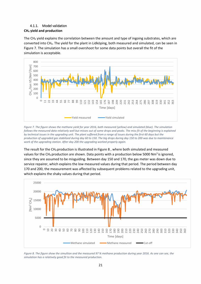
The measured data comes from 2016, which also is the data the model is validated against. During
the beging of 2016, the plant had some problems regarding the gas upgrade and certain amounts of
gas were flared during these periods. Since the raw gas meter has low credability, the simultion has
been validated against the upgraded gas. However, these values are affected by issues regardning
the upgrading system, which occurred during a time period. The upgrading system was maintenced
in middle of the year, which means that there was no or very low CH4 production during that period.
This explains the shape of the graphs in Figure 7 and Figure 8 for the measured data. Since the model
cannot predict these types of issues, data points below 5000 Nm3 have been ignored in the statistical
test.
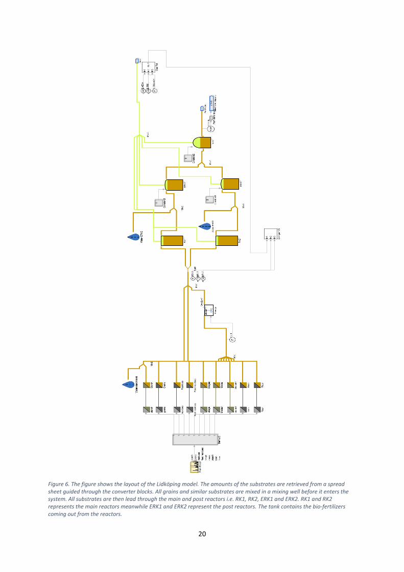
20
Figure 6. The figure shows the layout of the Lidköping model. The amounts of the substrates are retrieved from a spread sheet guided through the converter blocks. All grains and similar substrates are mixed in a mixing well before it enters the system. All substrates are then lead through the main and post reactors i.e. RK1, RK2, ERK1 and ERK2. RK1 and RK2 represents the main reactors meanwhile ERK1 and ERK2 represent the post reactors. The tank contains the bio-fertilizers coming out from the reactors.
21
4.1.1. Model validation
CH4 yield and production
The CH4 yield explains the correlation between the amount and type of ingoing substrates, which are
converted into CH4. The yield for the plant in Lidköping, both measured and simulated, can be seen in
Figure 7. The simulation has a small overshoot for some data points but overall the fit of the
simulation is acceptable.
Figure 7. The figure shows the methane yield for year 2016, both measured (yellow) and simulated (blue). The simulation follows the measured data relatively well but misses out of some drops and peaks. The miss fit of the beginning is explained by technical issues in the upgrading unit. The plant suffered from a range of issues during the first 60 days but the production of upgraded gas stabilized during day 60 to 150. The big drops during day 150 to 200 was due to maintenance work of the upgrading station. After day 200 the upgrading worked properly again.
The result for the CH4 production is illustrated in Figure 8 , where both simulated and measured
values for the CH4 production are shown. Data points with a production below 5000 Nm3 is ignored,
since they are assumed to be misguiding. Between day 150 and 170, the gas meter was down due to
service repairer, which explains the low measured values during that period. The period between day
170 and 200, the measurement was affected by subsequent problems related to the upgrading unit,
which explains the shaky values during that period.
Figure 8. The figure show the simultion and the measured 97 % methane production during year 2016. As one can see, the simulation has a relatively good fit to the measured production.
0
100
200
300
400
500
600
700
800
0
11
22
33
44
55
66
77
88
99
11
0
12
1
13
2
14
3
15
4
16
5
17
6
18
7
19
8
20
9
22
0
23
1
24
2
25
3
26
4
27
5
28
6
29
7
30
8
31
9
33
0
34
1
35
2
36
3
CH
4/t
on
VS
[Nm
3 /to
n]
Time [days]
Yield measured Yield simulated
0
5000
10000
15000
20000
25000
0
10
20
30
40
50
60
70
80
90
10
0
11
0
12
0
13
0
14
0
15
0
16
0
17
0
18
0
19
0
20
0
21
0
22
0
23
0
24
0
25
0
26
0
27
0
28
0
29
0
30
0
31
0
32
0
33
0
34
0
35
0
36
0
[Nm
3C
H4]
Time [days]
Methane simulated Methane measured Cut-off
22
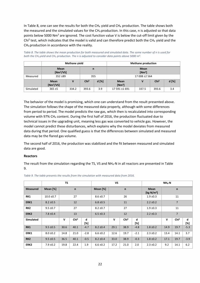
In Table 8, one can see the results for both the CH4 yield and CH4 production. The table shows both
the measured and the simulated values for the CH4 production. In this case, n is adjusted so that data
points below 5000 Nm3 are ignored. The cost function value V is below the cut-off limit given by the
Chi2 test, which indicates that the model is valid and can therefore predict both the CH4 yield and the
CH4 production in accordance with the reality.
Table 8. The table shows the mean production for both measured and simulated data. The same number of n is used for both the CH4 yield and CH4 production. The n is adjusted to consider data points above 5000 m3.
Methane yield Methane production
Mean [Nm3/VS]
n Mean [Nm3]
Measured 352 ±89 355 17 008 ±2 564
Mean [Nm3/VS]
V Chi2 d [%] Mean [Nm3]
V Chi2 d [%]
Simulated 365 ±5 334.2 393.6 3.9 17 591 ±1 691 337.5 393.6 3.4
The behavior of the model is promising, which one can understand from the result presented above.
The simulation follows the shape of the measured data properly, although with some differences
from period to period. The model predicts the raw gas, which then is recalculated into corresponding
volume with 97% CH4 content. During the first half of 2016, the production fluctuated due to
technical issues in the upgrading unit, meaning less gas was converted to vehicle gas. However, the
model cannot predict these disturbances, which explains why the model deviates from measured
data during that period. One qualified guess is that the differences between simulated and measured
data may be the flared gas volume.
The second half of 2016, the production was stabilized and the fit between measured and simulated
data are good.
Reactors
The result from the simulation regarding the TS, VS and NH4-N in all reactors are presented in Table
9.
Table 9. The table presents the results from the simulation with measured data from 2016.
TS VS NH4-N
Measured Mean [%] n Mean [%] n Mean [kg N/m3]
n
RK1 10.0 ±0.7 27 8.6 ±0.7 26 1.9 ±0.3 11
ERK1 8.2 ±0.5 12 6.8 ±0.5 11 2.2 ±0.2 7
RK2 9.5 ±0.7 27 8.2 ±0.7 27 1.9 ±0.3 11
ERK2 7.8 ±0.4 13 6.5 ±0.3 12 2.2 ±0.3 7
Simulated V Chi2 d [%]
V Chi2 d [%]
V Chi2 d [%]
RK1 9.5 ±0.5 30.6 40.1 -4.7 8.2 ±0.4 29.1 38.9 -4.8 1.8 ±0.2 14.9 19.7 -5.3
ERK1 8.0 ±0.2 14.8 21.0 -2.8 6.6 ±0.2 12.6 19.7 -2.1 2.3 ±0.2 13.4 14.1 3.7
RK2 9.5 ±0.5 36.5 40.1 -0.5 8.2 ±0.4 33.0 38.9 -0.3 1.8 ±0.2 17.1 19.7 -3.9
ERK2 7.9 ±0.2 19.8 22.4 1.9 6.6 ±0.2 17.2 21.0 2.0 2.3 ±0.2 9.2 14.1 6.2
23
Based on the result from the simulation and the statistical test, it can be stated that the model
behaves as desired for the predictions of TS, VS and NH4-N in all reactors. The credibility of the model
is strengthened by the results from the statistical test, where all V values is lower than corresponding
chi2 value. This indicates that the model is statistically justifiable for all measurements and the mean
difference d lays within reasonable ranges for all measurements as well.
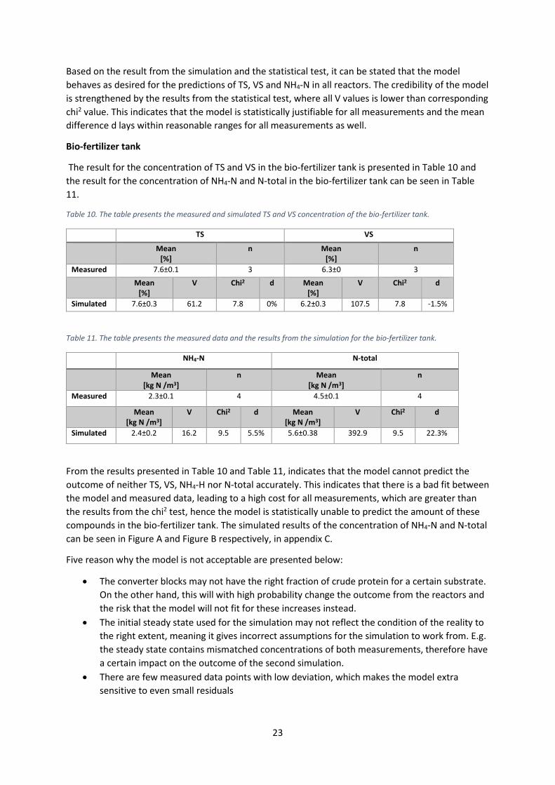
Bio-fertilizer tank
The result for the concentration of TS and VS in the bio-fertilizer tank is presented in Table 10 and
the result for the concentration of NH4-N and N-total in the bio-fertilizer tank can be seen in Table
11.
Table 10. The table presents the measured and simulated TS and VS concentration of the bio-fertilizer tank.
TS VS
Mean [%]
n Mean [%]
n
Measured 7.6±0.1 3 6.3±0 3
Mean [%]
V Chi2 d Mean [%]
V Chi2 d
Simulated 7.6±0.3 61.2 7.8 0% 6.2±0.3 107.5 7.8 -1.5%
Table 11. The table presents the measured data and the results from the simulation for the bio-fertilizer tank.
NH4-N N-total
Mean [kg N /m3]
n Mean [kg N /m3]
n
Measured 2.3±0.1 4 4.5±0.1 4
Mean [kg N /m3]
V Chi2 d Mean [kg N /m3]
V Chi2 d
Simulated 2.4±0.2 16.2 9.5 5.5% 5.6±0.38 392.9 9.5 22.3%
From the results presented in Table 10 and Table 11, indicates that the model cannot predict the
outcome of neither TS, VS, NH4-H nor N-total accurately. This indicates that there is a bad fit between
the model and measured data, leading to a high cost for all measurements, which are greater than
the results from the chi2 test, hence the model is statistically unable to predict the amount of these
compounds in the bio-fertilizer tank. The simulated results of the concentration of NH4-N and N-total
can be seen in Figure A and Figure B respectively, in appendix C.
Five reason why the model is not acceptable are presented below:
The converter blocks may not have the right fraction of crude protein for a certain substrate.
On the other hand, this will with high probability change the outcome from the reactors and
the risk that the model will not fit for these increases instead.
The initial steady state used for the simulation may not reflect the condition of the reality to
the right extent, meaning it gives incorrect assumptions for the simulation to work from. E.g.
the steady state contains mismatched concentrations of both measurements, therefore have
a certain impact on the outcome of the second simulation.
There are few measured data points with low deviation, which makes the model extra
sensitive to even small residuals
24
Additional reasons why the prediction fails is that the model does not consider the
fluctuation in volume or temperature of the bio-fertilizer tank. As previously mentioned, the
tank is used as buffer storage, which may affect the outcome of the result.
The N balance might be insufficiently handled by the mathematical model.
Summary: Validation of the Lidköping model
The model of the Lidköping plant shows promising results and the credibility for the predictions are
in the majority statistical justifiable, meaning the model is valid.
The prediction of both the CH4 yield and CH4 production corresponds to the outcome in
reality.
The prediction of the TS and VS values for all reactors are valid.
The model can predict the concentration of NH4-N for both the main and post reactors.
The simulation of the concentration of NH4-N in the post reactors have a higher agreement
with measured data compared to the same simulation for the concentration of NH4-N in the
main reactors.
The model is not statistically justifiable regarding the prediction of the concentration of NH4-
N and N-total in the bio-fertilizer tank. However, the model does not consider the fluctuating
volume or temperature of the bio-fertilizer tank.
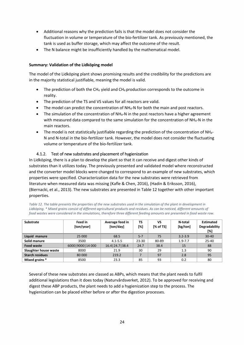
4.1.2. Test of new substrates and placement of hygienization
In Lidköping, there is a plan to develop the plant so that it can receive and digest other kinds of
substrates than it utilizes today. The previously presented and validated model where reconstructed
and the converter model blocks were changed to correspond to an example of new substrates, which
properties were specified. Characterization data for the new substrates were retrieved from
literature when measured data was missing (Kafle & Chen, 2016), (Hadin & Eriksson, 2016),
(Biernacki, et al., 2013). The new substrates are presented in Table 12 together with other important
properties.
Table 12. The table presents the properties of the new substrates used in the simulation of the plant in development in Lidköping. * Mixed grains consist of different agricultural products and residues. As can be noticed, different amounts of food wastes were considered in the simulations, therefore three different feeding amounts are presented in food waste row.
Substrate Feed in [ton/year]
Average feed in [ton/day]
TS [%]
VS [% of TS]
N-total [kg/ton]
Estimated Degradability
[%]
Liquid manure 25 000 68.5 5-7 75 3.2-3.9 30-40
Solid manure 3500 4.1-5.5 23-30 80-89 1.9-7.7 25-40
Food waste 6000|9000|14 000 16.4|24.7|38.4 24.7 38.4 15 88
Slaughter house waste 8000 21.9 30 29 1.3 90
Starch residues 80 000 219.2 7 97 2.8 95
Mixed grains * 8500 23.3 85 93 0.2 80
Several of these new substrates are classed as ABPs, which means that the plant needs to fulfil
additional legislations than it does today (Naturvårdsverket, 2012). To be approved for receiving and
digest these ABP products, the plant needs to add a hygienization step to the process. The
hygienization can be placed either before or after the digestion processes.
25
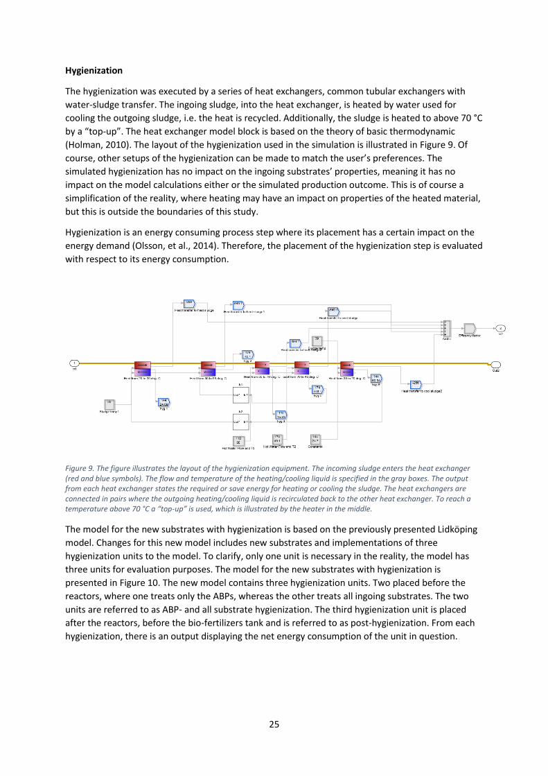
Hygienization
The hygienization was executed by a series of heat exchangers, common tubular exchangers with
water-sludge transfer. The ingoing sludge, into the heat exchanger, is heated by water used for
cooling the outgoing sludge, i.e. the heat is recycled. Additionally, the sludge is heated to above 70 °C
by a “top-up”. The heat exchanger model block is based on the theory of basic thermodynamic
(Holman, 2010). The layout of the hygienization used in the simulation is illustrated in Figure 9. Of
course, other setups of the hygienization can be made to match the user’s preferences. The
simulated hygienization has no impact on the ingoing substrates’ properties, meaning it has no
impact on the model calculations either or the simulated production outcome. This is of course a
simplification of the reality, where heating may have an impact on properties of the heated material,
but this is outside the boundaries of this study.
Hygienization is an energy consuming process step where its placement has a certain impact on the
energy demand (Olsson, et al., 2014). Therefore, the placement of the hygienization step is evaluated
with respect to its energy consumption.
Figure 9. The figure illustrates the layout of the hygienization equipment. The incoming sludge enters the heat exchanger (red and blue symbols). The flow and temperature of the heating/cooling liquid is specified in the gray boxes. The output from each heat exchanger states the required or save energy for heating or cooling the sludge. The heat exchangers are connected in pairs where the outgoing heating/cooling liquid is recirculated back to the other heat exchanger. To reach a temperature above 70 °C a “top-up” is used, which is illustrated by the heater in the middle.
The model for the new substrates with hygienization is based on the previously presented Lidköping
model. Changes for this new model includes new substrates and implementations of three
hygienization units to the model. To clarify, only one unit is necessary in the reality, the model has
three units for evaluation purposes. The model for the new substrates with hygienization is
presented in Figure 10. The new model contains three hygienization units. Two placed before the
reactors, where one treats only the ABPs, whereas the other treats all ingoing substrates. The two
units are referred to as ABP- and all substrate hygienization. The third hygienization unit is placed
after the reactors, before the bio-fertilizers tank and is referred to as post-hygienization. From each
hygienization, there is an output displaying the net energy consumption of the unit in question.
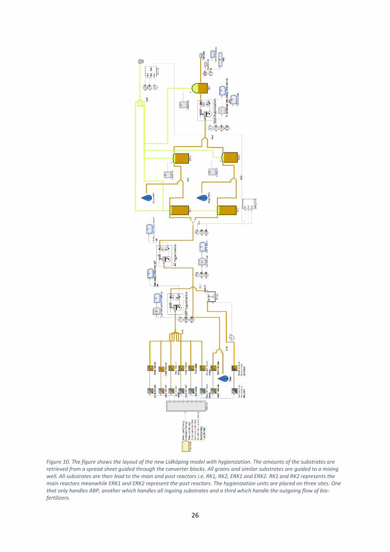
26
Figure 10. The figure shows the layout of the new Lidköping model with hygienization. The amounts of the substrates are retrieved from a spread sheet guided through the converter blocks. All grains and similar substrates are guided to a mixing well. All substrates are then lead to the main and post reactors i.e. RK1, RK2, ERK1 and ERK2. RK1 and RK2 represents the main reactors meanwhile ERK1 and ERK2 represent the post reactors. The hygienization units are placed on three sites. One that only handles ABP, another which handles all ingoing substrates and a third which handle the outgoing flow of bio-fertilizers.
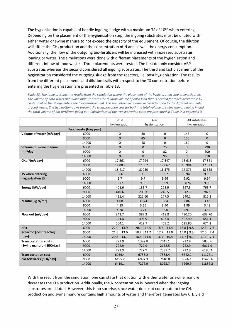
27
The hygienization is capable of handle ingoing sludge with a maximum TS of 10% when entering.
Depending on the placement of the hygienization step, the ingoing substrates must be diluted with
either water or swine manure to not exceed the capacity of the equipment. Of course, the dilution
will affect the CH4 production and the concentration of N and as well the energy consumption.
Additionally, the flow of the outgoing bio-fertilizers will be increased with increased substrates
loading or water. The simulations were done with different placements of the hygienization and
different inflow of food wastes. Three placements were tested. The first do only consider ABP
substrates whereas the second considered all ingoing substrates. The third and last placement of the
hygienization considered the outgoing sludge from the reactors, i.e. post hygienization. The results
from the different placements and dilution trails with respect to the TS concentration before
entering the hygienization are presented in Table 13.
Table 13. The table presents the results from the simulation where the placement of the hygienization step is investigated. The volume of both water and swine manure states the dilution volume of each kind that is needed for reach acceptable TS content when the sludge enters the hygienization unit. The simulation were done in consideration to the different amounts of food waste. The two bottom rows present the transportation cost for both the total volume of swine manure going in and the total volume of bio-fertilizers going out. Calculations of the transportation costs are presented in Table D in appendix D.
Post hygienization
ABP hygienization
All substrates hygienization
Food waste [ton/year]
Volume of water [m3/day] 6000 0 38 0 145 0
9000 0 45 0 150 0
14000 0 48 0 160 0
Volume of swine manure [m3/day]
6000 0 0 75 0 290
9000 0 0 82 0 300
14000 0 0 95 0 310
CH4 [Nm3/day]
6000 17 561 17 294 17 547 16 615 17 521
9000 17 883 17 567 17 862 16 904 17 823
14000 18 417 18 080 18 375 17 375 18 325
TS when entering hygienization [%]
6000 5.66 9.9 9.92 9.94 9.95
9000 5.7 9.7 9.96 9.92 9.94
14000 5.77 9.96 9.99 9.876 9.98
Energy [kW/day] 6000 401.6 185.7 228.9 597.3 766.7
9000 410.6 203.3 246.5 612.3 787.9
14000 425.4 222.60 277.5 640.1 815.3
N-total [kg N/m3] 6000 4.08 3.674 3.84 2.86 3.46
9000 4.13 3.66 3.90 2.89 3.48
14000 4.20 3.71 3.90 2.91 3.52
Flow out [m3/day] 6000 343.7 382.2 418.8 490.20 633.70
9000 351.4 396.9 433.4 502.90 651.1
14000 364.1 412.7 459.2 525.80 674.2
HRT (reactor |post reactor) [day]
6000 22.0 | 13.9 20.0 | 12.5 18.3 | 11.4 15.8 | 9.8 12.3 | 7.6
9000 21.6 | 13.6 18.7 | 11.7 17.7 | 11.0 15.0 | 9.3 12.0 | 7.4
14000 20.8 | 13.1 18.5 | 11.6 16.7 | 10.4 14.7 | 9.1 11.6 | 7.1
Transportation cost in (Swine manure) [SEK/day]
6000 722.9 1392.8 2045.1 722.9 5835.6
9000 722.9 722.9 2168.5 722.9 6011.9
14000 722.9 722.9 2397.7 722.9 6188.2
Transportation cost bio-fertilizers [SEK/day]
6000 6059.4 6738.2 7383.4 8642.2 11172.1
9000 6195.2 6997.3 7640.8 8866.1 11479.6
14000 6419.1 7275.9 8095.7 9269.9 11886.2
With the result from the simulation, one can state that dilution with either water or swine manure
decreases the CH4 production. Additionally, the N concentration is lowered when the ingoing
substrates are diluted. However, this is no surprise, since water does not contribute to the CH4
production and swine manure contains high amounts of water and therefore generates low CH4 yield
28
(Angelidaki & Ellegaard, 2003). This can be related to the decreasing HRT when the dilution volume
increases. Therefore, the best CH4 production is reached when no dilution is done.
In the case with no dilution, the placement of the hygienization must be after the reactors i.e. post
hygienization. This is due to the boundaries of the hygienization, which cannot handle TS
concentrations over 10%. Additionally, this gives the lowest outflow of bio-fertilizers with the
highest concentration of N, meaning the transportation costs of the bio-fertilizers are kept low,
compared to the cases where dilution is needed.
Post hygienization has also the advantage of easily being adapted to introduction of new substrates.
This is since the post hygienization has more capacity left regarding the handling of the TS content in
the sludge compared to the pre hygenizers.
The drawback with the post-hygienization is the high-energy consumption compared to the ABP
hygienization.
If pre-hygienization is considered, dilution is needed. It seems rather unnecessary to let all ingoing
substrates go through hygienization both from an energy and substrate supply perspective.
Therefore, ABP hygienization is favored when choosing between these two alternatives. It is also
better to use swine manure over water since it does not only dilute the sludge, it also contributes a
bit to the CH4 production.
It can also be stated that to reach an acceptable concentration of TS in the case of pre hygienization,
there will be a need of addition of a certain volume of either swine manure or water to the system.
This leads to an increased outflow of bio-fertilizers, which must be stored and transported.
Additionally, this will accordingly to the simulations also deteriorates both the CH4 production and
the quality of the bio-fertilizers.
The problem with the dilution is that large volumes of either swine manure or water must be added
to the system, which would lead to increased transportation costs. Of course, the dilution with swine
manure requires a continuous supply, which can be added to the system daily. If there is a lack of
swine manure for some reason, the production must be degraded and adjusted to match the
boundaries of the hygienization unit.
Despite the drawback with high energy consumption, post-hygienization is the best alternative to
implement to the system. This setup together with the new substrates gives equal or better CH4
production compared to the measured data from 2016.
29
4.2. KATRINEHOLM The model of the plant in Katrineholm consists of eleven different substrates, where each is specified
in converter blocks. The feed pattern is retrieved from a spread sheet, where each column contains
the amount of substrate expressed in ton per day. In accordance with reality, the model has two
reactors, which both converge to a fertilizers storage. Gas is acquired from the two reactors but not
from the fertilizer storage. The reactors are denoted RK1 and RK2 respectively. The layout of the
Katrineholm plant model is presented in Figure 11. The plant has had some issues regarding the
measurement meters and the production during a period, which has been considered in the
validation.
The simulated results and their correlation with measured data are presented below.
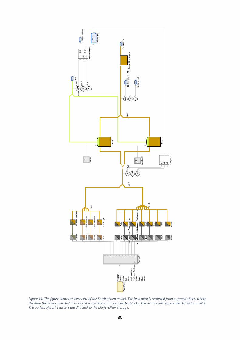
30
Figure 11. The figure shows an overview of the Katrineholm model. The feed data is retrieved from a spread sheet, where the data then are converted in to model parameters in the converter blocks. The rectors are represented by RK1 and RK2. The outlets of both reactors are directed to the bio-fertilizer storage.
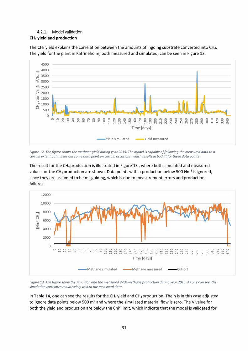
31
4.2.1. Model validation
CH4 yield and production
The CH4 yield explains the correlation between the amounts of ingoing substrate converted into CH4.
The yield for the plant in Katrineholm, both measured and simulated, can be seen in Figure 12.
Figure 12. The figure shows the methane yield during year 2015. The model is capable of following the measured data to a certain extent but misses out some data point on certain occasions, which results in bad fit for these data points
The result for the CH4 production is illustrated in Figure 13 , where both simulated and measured
values for the CH4 production are shown. Data points with a production below 500 Nm3 is ignored,
since they are assumed to be misguiding, which is due to measurement errors and production
failures.
Figure 13. The figure show the simultion and the measured 97 % methane production during year 2015. As one can see. the simulation correlates realativelely well to the measuerd data
In Table 14, one can see the results for the CH4 yield and CH4 production. The n is in this case adjusted
to ignore data points below 500 m3 and where the simulated material flow is zero. The V value for
both the yield and production are below the Chi2 limit, which indicate that the model is validated for
0
500
1000
1500
2000
2500
3000
3500
4000
4500
0
10
20
30
40
50
60
70
80
90
10
0
11
0
12
0
13
0
14
0
15
0
16
0
17
0
18
0
19
0
20
0
21
0
22
0
23
0
24
0
25
0
26
0
27
0
28
0
29
0
30
0
31
0
32
0
33
0
34
0
CH
4/t
on
VS
[Nm
3 /to
n]
Time [days]
Yield simulated Yield measured
0
2000
4000
6000
8000
10000
12000
0
10
20
30
40
50
60
70
80
90
10
0
11
0
12
0
13
0
14
0
15
0
16
0
17
0
18
0
19
0
20
0
21
0
22
0
23
0
24
0
25
0
26
0
27
0
28
0
29
0
30
0
31
0
32
0
33
0
34
0
[Nm
3C
H4]
Time [days]
Methane simulated Methane measured Cut-off
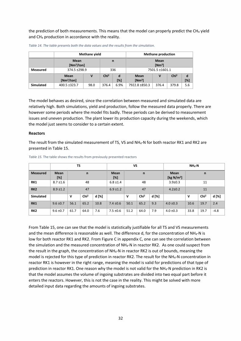
32
the prediction of both measurements. This means that the model can properly predict the CH4 yield
and CH4 production in accordance with the reality.
Table 14. The table presents both the data values and the results from the simulation.
Methane yield Methane production
Mean [Nm3/ton]
n Mean [Nm3]
Measured 374.5 ±298.9 336 7501.5 ±1601.1
Mean [Nm3/ton]
V Chi2 d [%]
Mean [Nm3]
V Chi2 d [%]
Simulated 400.5 ±323.7 98.0 376.4 6.9% 7922.8 ±850.3 376.4 379.8 5.6
The model behaves as desired, since the correlation between measured and simulated data are
relatively high. Both simulations, yield and production, follow the measured data properly. There are
however some periods where the model fits badly. These periods can be derived to measurement
issues and uneven production. The plant lower its production capacity during the weekends, which
the model just seems to consider to a certain extent.
Reactors
The result from the simulated measurement of TS, VS and NH4-N for both reactor RK1 and RK2 are
presented in Table 15.
Table 15. The table shows the results from previously presented reactors
TS VS NH4-N
Measured Mean [%]
n Mean [%]
n Mean [kg N/m3]
n
RK1 8.7 ±1.6 48 6.8 ±1.4 48 3.9±0.3 11
RK2 8.9 ±1.2 47 6.9 ±1.2 47 4.2±0.2 11
Simulated V Chi2 d [%] V Chi2 d [%] V Chi2 d [%]
RK1 9.6 ±0.7 56.1 65.2 10.8 7.4 ±0.6 50.1 65.2 9.3 4.0 ±0.3 10.6 19.7 2.4
RK2 9.6 ±0.7 61.7 64.0 7.6 7.5 ±0.6 51.2 64.0 7.9 4.0 ±0.3 33.8 19.7 -4.8
From Table 15, one can see that the model is statistically justifiable for all TS and VS measurements
and the mean difference is reasonable as well. The difference d, for the concentration of NH4-N is
low for both reactor RK1 and RK2. From Figure C in appendix C, one can see the correlation between
the simulation and the measured concentration of NH4-N in reactor RK2. As one could suspect from
the result in the graph, the concentration of NH4-N in reactor RK2 is out of bounds, meaning the
model is rejected for this type of prediction in reactor RK2. The result for the NH4-N concentration in
reactor RK1 is however in the right range, meaning the model is valid for predictions of that type of
prediction in reactor RK1. One reason why the model is not valid for the NH4-N prediction in RK2 is
that the model assumes the volume of ingoing substrates are divided into two equal part before it
enters the reactors. However, this is not the case in the reality. This might be solved with more
detailed input data regarding the amounts of ingoing substrates.
33
Bio-fertilizer storage
The result for the bio-fertilizer storage are presented in Table 16 and the results from the simulation
of the measurement of NH4-N and N-total in the bio-fertilizers are presented in Table 17.
Table 16. The table presents the concentration of TS and VS for both measured and simulated data.
TS VS
Mean [%]
n Mean [%]
n
Measured 8.5 ±1.2 11 6.6 ±1.1 11
Mean [%]
V Chi2 d Mean [%]
V Chi2 d
Simulated 8.6 ±1.1 10.2 19.7 2% 6.6 ±0.8 7.7 19.7 1%
From the result in Table 16, it is clear that the model can predict the concentration of both TS and VS
in the bio-fertilizer storage. The deviation between measured and simulated is small. Additionally,
the model is valid, since it is not rejected by the Chi2 test.
Table 17. The table presents the results for both measured and simulated data.
NH4-N N-total
Mean [kg N/m3]
n Mean [kg N/m3]
n
Measured 4.1 ±0.17 11 6.8 ±0.5 11
Mean [kg N/m3]
V Chi2 d Mean [kg N/m3]
V Chi2 d
Simulated 4.05 ±0.3 23.6 19.7 -1.3% 6.8 ±0.5 9.0 19.7 0%
As can be seen in Table 17, it can be stated that the model fails to predict the concentration of NH4-N
to the right extent i.e. there is a bad fit between simulated and measured data. The prediction of the
concentration of NH4-N is not valid since the V is too big. However, this difference is not that big and
the d-value lies in reasonable range. The result of the simulated NH4-N concentration can be seen in
Figure D in appendix C.
However, the model is capable of predict the N-total concentration, meaning the model is valid for
that type of prediction.
Summary: Validation of the Katrineholm model
The model of Katrineholm is validated for the yield and production of CH4. The model can
predict the TS and VS concentration as well to statistical justification.
The model can predict the concentration of NH4-N in reactor RK1 but the prediction in
reactor RK2 is not acceptable.
The model can predict the TS, VS and N-total concentration for the bio-fertilizers but is not
valid for the prediction of the NH4-N concentration.
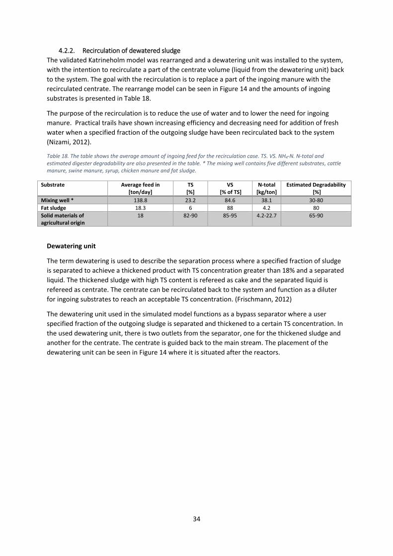
34
4.2.2. Recirculation of dewatered sludge
The validated Katrineholm model was rearranged and a dewatering unit was installed to the system,
with the intention to recirculate a part of the centrate volume (liquid from the dewatering unit) back
to the system. The goal with the recirculation is to replace a part of the ingoing manure with the
recirculated centrate. The rearrange model can be seen in Figure 14 and the amounts of ingoing
substrates is presented in Table 18.
The purpose of the recirculation is to reduce the use of water and to lower the need for ingoing
manure. Practical trails have shown increasing efficiency and decreasing need for addition of fresh
water when a specified fraction of the outgoing sludge have been recirculated back to the system
(Nizami, 2012).
Table 18. The table shows the average amount of ingoing feed for the recirculation case. TS. VS. NH4-N. N-total and estimated digester degradability are also presented in the table. * The mixing well contains five different substrates, cattle manure, swine manure, syrup, chicken manure and fat sludge.
Substrate Average feed in [ton/day]
TS [%]
VS [% of TS]
N-total [kg/ton]
Estimated Degradability [%]
Mixing well * 138.8 23.2 84.6 38.1 30-80
Fat sludge 18.3 6 88 4.2 80
Solid materials of agricultural origin
18 82-90 85-95 4.2-22.7 65-90
Dewatering unit
The term dewatering is used to describe the separation process where a specified fraction of sludge
is separated to achieve a thickened product with TS concentration greater than 18% and a separated
liquid. The thickened sludge with high TS content is refereed as cake and the separated liquid is
refereed as centrate. The centrate can be recirculated back to the system and function as a diluter
for ingoing substrates to reach an acceptable TS concentration. (Frischmann, 2012)
The dewatering unit used in the simulated model functions as a bypass separator where a user
specified fraction of the outgoing sludge is separated and thickened to a certain TS concentration. In
the used dewatering unit, there is two outlets from the separator, one for the thickened sludge and
another for the centrate. The centrate is guided back to the main stream. The placement of the
dewatering unit can be seen in Figure 14 where it is situated after the reactors.
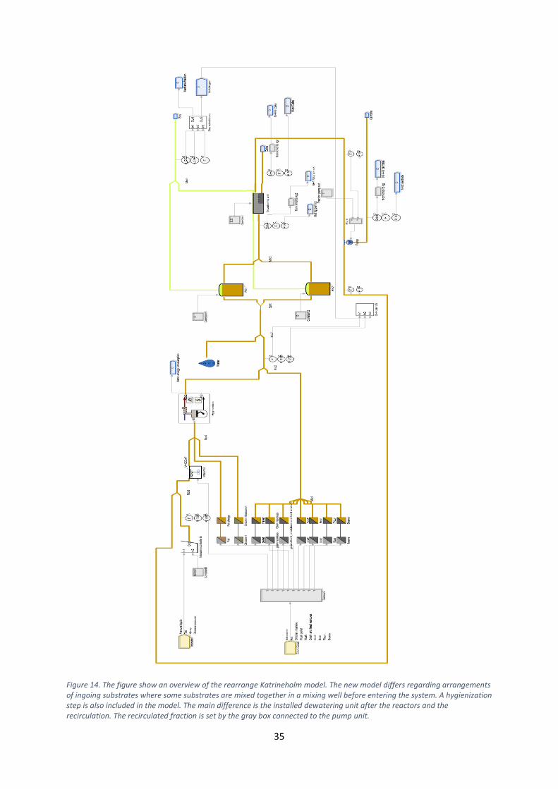
35
Figure 14. The figure show an overview of the rearrange Katrineholm model. The new model differs regarding arrangements of ingoing substrates where some substrates are mixed together in a mixing well before entering the system. A hygienization step is also included in the model. The main difference is the installed dewatering unit after the reactors and the recirculation. The recirculated fraction is set by the gray box connected to the pump unit.
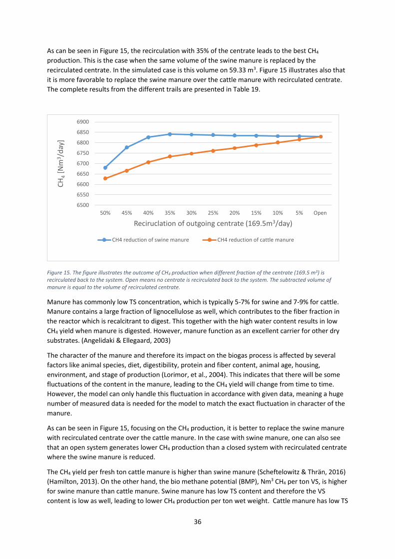
36
As can be seen in Figure 15, the recirculation with 35% of the centrate leads to the best CH4
production. This is the case when the same volume of the swine manure is replaced by the
recirculated centrate. In the simulated case is this volume on 59.33 m3. Figure 15 illustrates also that
it is more favorable to replace the swine manure over the cattle manure with recirculated centrate.
The complete results from the different trails are presented in Table 19.
Figure 15. The figure illustrates the outcome of CH4 production when different fraction of the centrate (169.5 m3) is recirculated back to the system. Open means no centrate is recirculated back to the system. The subtracted volume of manure is equal to the volume of recirculated centrate.
Manure has commonly low TS concentration, which is typically 5-7% for swine and 7-9% for cattle.
Manure contains a large fraction of lignocellulose as well, which contributes to the fiber fraction in
the reactor which is recalcitrant to digest. This together with the high water content results in low
CH4 yield when manure is digested. However, manure function as an excellent carrier for other dry
substrates. (Angelidaki & Ellegaard, 2003)
The character of the manure and therefore its impact on the biogas process is affected by several
factors like animal species, diet, digestibility, protein and fiber content, animal age, housing,
environment, and stage of production (Lorimor, et al., 2004). This indicates that there will be some
fluctuations of the content in the manure, leading to the CH4 yield will change from time to time.
However, the model can only handle this fluctuation in accordance with given data, meaning a huge
number of measured data is needed for the model to match the exact fluctuation in character of the
manure.
As can be seen in Figure 15, focusing on the CH4 production, it is better to replace the swine manure
with recirculated centrate over the cattle manure. In the case with swine manure, one can also see
that an open system generates lower CH4 production than a closed system with recirculated centrate
where the swine manure is reduced.
The CH4 yield per fresh ton cattle manure is higher than swine manure (Scheftelowitz & Thrän, 2016)
(Hamilton, 2013). On the other hand, the bio methane potential (BMP), Nm3 CH4 per ton VS, is higher
for swine manure than cattle manure. Swine manure has low TS content and therefore the VS
content is low as well, leading to lower CH4 production per ton wet weight. Cattle manure has low TS
6500
6550
6600
6650
6700
6750
6800
6850
6900
50% 45% 40% 35% 30% 25% 20% 15% 10% 5% Open
CH
4[N
m3/d
ay]
Reciruclation of outgoing centrate (169.5m3/day)
CH4 reduction of swine manure CH4 reduction of cattle manure
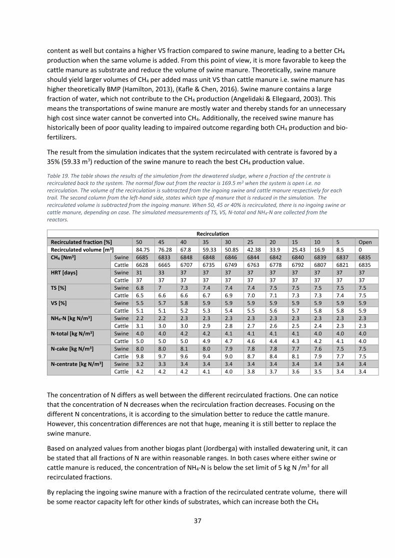
37
content as well but contains a higher VS fraction compared to swine manure, leading to a better CH4
production when the same volume is added. From this point of view, it is more favorable to keep the
cattle manure as substrate and reduce the volume of swine manure. Theoretically, swine manure
should yield larger volumes of CH4 per added mass unit VS than cattle manure i.e. swine manure has
higher theoretically BMP (Hamilton, 2013), (Kafle & Chen, 2016). Swine manure contains a large
fraction of water, which not contribute to the CH4 production (Angelidaki & Ellegaard, 2003). This
means the transportations of swine manure are mostly water and thereby stands for an unnecessary
high cost since water cannot be converted into CH4. Additionally, the received swine manure has
historically been of poor quality leading to impaired outcome regarding both CH4 production and bio-
fertilizers.
The result from the simulation indicates that the system recirculated with centrate is favored by a
35% (59.33 m3) reduction of the swine manure to reach the best CH4 production value.
Table 19. The table shows the results of the simulation from the dewatered sludge, where a fraction of the centrate is recirculated back to the system. The normal flow out from the reactor is 169.5 m3 when the system is open i.e. no recirculation. The volume of the recirculation is subtracted from the ingoing swine and cattle manure respectively for each trail. The second column from the left-hand side, states which type of manure that is reduced in the simulation. The recirculated volume is subtracted from the ingoing manure. When 50, 45 or 40% is recirculated, there is no ingoing swine or cattle manure, depending on case. The simulated measurements of TS, VS, N-total and NH4-N are collected from the reactors.
Recirculation
Recirculated fraction [%] 50 45 40 35 30 25 20 15 10 5 Open
Recirculated volume [m3] 84.75 76.28 67.8 59.33 50.85 42.38 33.9 25.43 16.9 8.5 0
CH4 [Nm3]
Swine 6685 6833 6848 6848 6846 6844 6842 6840 6839 6837 6835
Cattle 6628 6665 6707 6735 6749 6763 6778 6792 6807 6821 6835
HRT [days] Swine 31 33 37 37 37 37 37 37 37 37 37
Cattle 37 37 37 37 37 37 37 37 37 37 37
TS [%] Swine 6.8 7 7.3 7.4 7.4 7.4 7.5 7.5 7.5 7.5 7.5
Cattle 6.5 6.6 6.6 6.7 6.9 7.0 7.1 7.3 7.3 7.4 7.5
VS [%] Swine 5.5 5.7 5.8 5.9 5.9 5.9 5.9 5.9 5.9 5.9 5.9
Cattle 5.1 5.1 5.2 5.3 5.4 5.5 5.6 5.7 5.8 5.8 5.9
NH4-N [kg N/m3] Swine 2.2 2.2 2.3 2.3 2.3 2.3 2.3 2.3 2.3 2.3 2.3
Cattle 3.1 3.0 3.0 2.9 2.8 2.7 2.6 2.5 2.4 2.3 2.3
N-total [kg N/m3] Swine 4.0 4.0 4.2 4.2 4.1 4.1 4.1 4.1 4.0 4.0 4.0
Cattle 5.0 5.0 5.0 4.9 4.7 4.6 4.4 4.3 4.2 4.1 4.0
N-cake [kg N/m3] Swine 8.0 8.0 8.1 8.0 7.9 7.8 7.8 7.7 7.6 7.5 7.5
Cattle 9.8 9.7 9.6 9.4 9.0 8.7 8.4 8.1 7.9 7.7 7.5
N-centrate [kg N/m3] Swine 3.2 3.3 3.4 3.4 3.4 3.4 3.4 3.4 3.4 3.4 3.4
Cattle 4.2 4.2 4.2 4.1 4.0 3.8 3.7 3.6 3.5 3.4 3.4
The concentration of N differs as well between the different recirculated fractions. One can notice
that the concentration of N decreases when the recirculation fraction decreases. Focusing on the
different N concentrations, it is according to the simulation better to reduce the cattle manure.
However, this concentration differences are not that huge, meaning it is still better to replace the
swine manure.
Based on analyzed values from another biogas plant (Jordberga) with installed dewatering unit, it can
be stated that all fractions of N are within reasonable ranges. In both cases where either swine or
cattle manure is reduced, the concentration of NH4-N is below the set limit of 5 kg N /m3 for all
recirculated fractions.
By replacing the ingoing swine manure with a fraction of the recirculated centrate volume, there will
be some reactor capacity left for other kinds of substrates, which can increase both the CH4
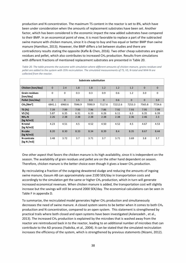
38
production and N concentration. The maximum TS content in the reactor is set to 8%, which have
been under consideration when the amounts of replacement substrates have been set. Another
factor, which has been considered is the economic impact the new added substrates have compared
to their BMP. In an economical point of view, it is most favorable to replace a part of the subtracted
swine manure with chicken manure, since it is cheap to buy and has equal or better BMP than swine
manure (Hamilton, 2013). However, the BMP differs a lot between studies and there are
contradictory results stating the opposite (Kafle & Chen, 2016). Two other cheap substrates are grain
residues and pellet, which also contributes to increased CH4 production. Results from simulations
with different fractions of mentioned replacement substrates are presented in Table 20.
Table 20. The table presents the outcome with simulation where different amounts of chicken manure, grains residues and pellet are added to the system with 35% recirculation. The simulated measurements of TS, VS, N-total and NH4-N are collected from the reactor.
Substrate substitution
Chicken [ton/day] 0 2.4 1.8 1.8 1.2 1.2 1.2 0 0
Grain residues [ton/day]
0 0 0.3 0.3 0.9 0.6 1.2 3.0 0
Pellet [ton/day] 0 0 1.5 0.3 0 0.6 0 0 3.0
CH4 [Nm3] 6841.1 6960.6 7046.9 7090.9 7117.6 72212.6 7253.3 7565.8 7724.6
TS [%] 7.39 7.99 7.93 7.96 7.86 7.92 7.93 7.95 7.99
VS [%] 5.87 6.35 6.31 6.33 6.26 6.11 6.3 6.35 6.39
NH4-N [kg N/m3]
2.26 2.38 2.38 2.38 2.38 2.38 2.36 2.46 2.3
N-total [kg N/m3]
4.23 4.51 4.5 4.52 4.50 4.52 4.5 4.67 4.53
N-cake [kg N/m3]
8.20 8.30 8.33 8.34 8.39 8.4 8.35 8.67 8.44
N-centrate [kg N /m3]
3.48 3.72 3.7 3.71 3.7 3.71 3.69 3.8 3.7
One other aspect that favors the chicken manure is its high availability, since it is independent on the
season. The availability of grain residues and pellet are on the other hand dependent on season.
Therefore, chicken manure is the better choice even though it gives a lower CH4 production.
By recirculating a fraction of the outgoing dewatered sludge and reducing the amounts of ingoing
swine manure, Gasum AB can approximately save 2100 SEK/day in transportation costs and
accordingly to the simulation get the same or higher CH4 production, which in turn will generate
increased economical revenues. When chicken manure is added, the transportation cost will slightly
increase but the savings will still be around 2000 SEK/day. The economical calculations can be seen in
Table F in appendix D.
To summarize, the recirculated model generates higher CH4 production and simultaneously
decreases the need of swine manure. A closed system seems to be better when it comes to both CH4
production and N concentration, compared to an open system. This statement is strengthened by
practical trails where both closed and open systems have been investigated (Aslanzadeh , et al.,
2013). The increased CH4 production is explained by the microbes that is washed away from the
reactor are reintroduced back in to the reactor, leading to an additional number of microbes that can
contribute to the AD process (Yadvika, et al., 2004). It can be stated that the simulated recirculation
increases the efficiency of the system, which is strengthened by previous statements (Nizami, 2012).
39
Unfortunately, there is a lack of measured data where this kind of recirculation is used in practice,
meaning the outcome of the simulation is rather uncertain. To really strength and verify the result,
one would need to conduct a pilot test and evaluate the impact of the recirculation with the centrate
and compare that data to the output from the model.
4.3. SUMMARY OF RESULTS AND ADDITIONAL COMMENTS
Modeling of existing biogas plants and corresponding simulated results indicates that it is possible to
create models with SIMBA#Biogas and ADM1, which agrees to measured data to the right extent.
The production of CH4 in both created models are simulated with a low percentage of deviation,
which goes in accordance with the result from similar work (Fronk, et al., 2014), (Biernacki, et al.,
2013), (Satpathy, et al., 2013). Both models can handel the concentrtion of TS and VS accuertely as
well. However, the prediction regardning the concentration of NH4-N are in some cases out of range,
meaning there is room for further improvments in the underlaying model, possibly regardning the N
balance.
SIMBA#Biogas is a powerfull tool and aid when one wants to predict the biogas process and the
results from this executed project proves that. However, the N concentration seems to be
unbalanced or not detailed enough to match the reality to the right extent, leadning to uncertain
results.
SIMBA#Biogas can function as an aid when it comes to choose which substrate that should be bought
and which should be ignored, since by specifying the properties of the substrates in the model, one
can estimate and predict how they will affect the process. SIMBA#Biogas is also cabaple of simulating
conditions where the system crashes, meaning knowledge to aviod failures can be obtained and
what causes them.
One drawback with ADM1da and therfore also SIMBA#Biogas is the input infromation about the
substrates, which are fearly excessive. Since this data is diffcult to meansure and obtaine, the model
will in some cases be based on estimations, meaning the output will be affected and therefore
yielding uncertain results.
On the othere hand, one has to keep in mind that a model is a simiplification of the reality and there
will always be devations between model and reality. Compared to other estimation methods, like
caluclations in Excel, SIMBA#Biogas offers a better overview and the risk that not all componets in
the process are considered is elimnated. The predictions will also be more detailed and therby can
optimization sites or failiures easier be spotted.
40
5. CONCLUSION
Modeling and simulation of the biogas plants in Lidköping and Katrineholm was executed with
promising results. Both models are capable of estimating the CH4 production, CH4 yield, TS and VS
concentration corresponding to the reality, meaning these values are statistically valid. Regarding the
NH4-N and N-total concentration, there are in some cases deviations between measured and
simulated data, making the model statistical unjustifiable.
The Lidköping model is able to predict the CH4 yield and CH4 production properly. TS and VS
concentrations are as well accurately simulated. The prediction of the TS, VS, NH4-N and N-total
concentration in the bio-fertilizer tank are deviating from measured data and are therefore not
trustworthy. The deviation can be derived to the fluctuation in the bio-fertilizer tank’s volume, which
the model does not consider to the right extent.
The Katrineholm model is able to predict the CH4 yield and CH4 production right. TS and VS
concentration values are as well properly simulated. The prediction of N-total concentration is as
desired but the model fails to predict the concentration of NH4-N properly.
The validated models where later rearrange where new substrates and equipment were tested. The
Lidköping model where tested with new substrates and three different placements of the
hygienization step. From an economical and practical point of view, post hygienization is
recommended over pre hygienization, since no dilution is needed and higher CH4 production and
thereby better economical profits can be achieved.
The Katrineholm model was implemented with a dewatering unit where a fraction of the centrate
was recirculated to the system. The result from the simulation indicates that the process is favored
by a 35% recirculation of the centrate volume, which substitutes the ingoing swine manure, yielding
better CH4 production and decreasing transportation costs. Both the TS and the NH4-N
concentrations in the reactors have been kept below 8% and 5 kg N/m3 respectively for all
recirculated fractions.
It can from this point be stated that modeling and simulations with SIMBA#Biogas and ADM1da are
an aid for the predictions of CH4 production when different wastes materials from the society are
been utilized in the biogas process. Knowledge how to utilize and combined these substrates to
reach the best CH4 yield will favor the society in the long term, since wastes’ value will be highlighted
and considered. This will hopefully give better energy efficiency and contribute to solve future rising
energy demands. Hence, one can conclude that modeling and simulation of an existing biogas plant
with satisfying agreement with the reality is possible with SIMBA#Biogas. Combined with the right
measured data, SIMBA#Biogas can function as a competent and powerful tool for estimation,
prediction and optimization of the overall biogas process.
For further work it is recommended with extensive analysis of substrates where parameters for
proper characterization are obtained. This should include the fractionation of COD, disintegration
rate of VS and the Weender parameters. Hopefully, this will reduce the uncertainty between
simulation and reality and yielding a fully functioning model. For proper validation of the models with
both the hygienization and the recirculation, pilot trails and further evaluations of these equipment’s
impact on the process are needed to be executed.
41
6. ACKNOWLEDGEMENT
There are several people I would like to acknowledge for their contribution to this project.
First, I would like to thank my family and friends for all your support and for believing in me.
Gasum AB Sweden for giving me the opportunity and possibility to do this project. A special thanks to
the staff at the office for your interest and for including me in the work team.
Thanks to Oliver Schraa, CTO at InCRTL Solutions Inc for putting up with my numerous questions and
for taking the time to explain and answer them. I am grateful for your support.
Thanks to my examiner Carl-Fredrik Mandenius, at IFM, LiU and Robert Gustavsson, supervisor at
IFM, LiU for taking on this project and for their guidance and valuable inputs during this time.
Thanks to my opponent Tom Axelsson, for providing me with relevant and helpful feedback to this
project.
Last, but not least I would like to thank my supervisor at Gasum AB, Anneli Ahlström for her
engagement, support and for pushing me forward. This project had not been completed without
your knowledge.
42
7. REFERENCES
Akbas, H., Bilgen, B. & Turham, A. M., 2015. An integrated prediction and optimization model of
biogas production system at a wastewater treatment facility. Bioresource Technolgy , Volume 196,
pp. 566-576.
Angelidaki, I. & Ellegaard, L., 2003. Codigestion of Manure and Organic Wastes in Centralized Biogas
Plants: Status and Future Trends. Applied Biochemistry and Biotechnology, 109(2003), pp. 95-105.
Angelidaki, I. et al., 2011. Biomethanation and its potential. Methanogenic Process: Microbiology,
Pathways, Applications. In: A. C. Rosenzweig & S. W. Ragsdale, eds. In Methods in Enzymology,
Methods in Methane Metabolism, Part A, Methanogenesis. San Diego: Elsevier inc, pp. 328-347.
Appels, L., Baeyens, J., Degre`ve, J. & Dewil, R., 2008. Principles and potential of the anaerobic
digestion of waste-activated sludge. Progress in Energy and Combustion Science, Volume 34, pp. 755-
781.
Arnell, M., 2016. Performance Assessment of Wastewater Treatment Plants : Multi-Objective Analysis
Using Plant-Wide Models. 1 ed. Lund: Lund University.
Arnell, M. et al., 2016. Modelling anaerobic co-digestion in Benchmark Simulation Model No. 2:
Parameter estimation, substrate characterisation and plant-wide integration.. Water Research,
Volume 98, pp. 138-146.
Aslanzadeh , S., Karthik , R., Jeihanipour, A. & Taherzadeh , M. J., 2013. The Effect of Effluent
Recirculation in a Semi-Continuous Two-Stage Anaerobic Digestion System. Energies, 6(1), pp. 2966-
2981.
Batstone, D. J., Keller, J., Angelidaki, I. & Kal, S. V., 2002. The IWA Anaerobic Digestion Model No 1
(ADM1). Water Science and Technology, 45(10), pp. 65-73.
Biernacki, P. et al., 2013. Application of Anaerobic Digestion Model No. 1 for descibing an exisiting
biogas power plant. Biomass and Bioenergy, Volume 59, pp. 441-447.
Biernacki, P., Steinigeweg, S., Borchert, A. & Uhlenhut, F., 2013. Application of Anaerobic Digestion
Model No. 1 for describing anaerobic digestion of grass, maize, green weed silage, and industrial
glycerine. Bioresource Technology, 127(1), pp. 188-194.
Blumensaat, F. & Keller, J., 2004. Modelling of two-stage anaerobic digestion using the IWA
Anaerobic Digestion Model No. 1 (ADM1). Water Research, 39(1), pp. 171-183.
Cedersund, G. & Roll, J., 2009. Systems biology: model based evaluation and comparison of potential
explanations for given biological data. The FEBS, Volume 276, pp. 903-922.
Chen, Y., 2008. Inhibition of anaerobic digestion process: A review. Bioresource Technology , Volume
99, pp. 4044-4064.
de Mes, T. Z., Stams, A. J., Reith, J. H. & Zeeman, G., 2003. Methane production by anaerobic
digestion of wastewater and solid wastes. In: R. W. a. H. B. J.H. Reith, ed. Bio-methane & Bio-
hydrogen - status and perspectives of biological methane and hydrogen production. Hague: Dutch
Biological Hydrogen Foundation, c/o Energy research Centre of The Netherlands ECN, Unit Biomass,
attn. J.H. Reith secretary, P.O., pp. 58-86.
43
Frischmann, P., 2012. Enhancement and treatment of digestates from anaerobic digestion, Oxon:
WRAP.
Fronk, K., Oguerk, M. & I, S., 2014. Modeling and simulation of biogas plants for representation of
important specific parameters. Stuttgart , ifaK, pp. 1-4.
Galí, A., Benabdallah, T., Astals, S. & Mata-Alvare, J., 2008. Modified version of ADM1 model for agro-
waste application. Bioresource Technology, Volume 100, pp. 2783-2790.
Gasum AB, 2017. Våra anläggningar. [Online]
Available at: https://www.gasum.com/sv/biogasanlaggningar/vara-anlaggningar/
[Accessed 25 04 2017].
Gerardi, M. H., 2003. Part 1 Overview. In: M. H. Gerardi, ed. The Microbiology of Anaerobic Digesters.
Haboken: John Wiley & Sons, pp. 1-58.
Grimsby, L. K., Fjørtoft, K. & Aune, J. B., 2013. Nitrogen mineralization and energy from anaerobic
digestion of jatropha press cake. Energy for Sustainable Development, 17(1), pp. 35-39.
Hadin, Å. & Eriksson, O., 2016. Horse manure as feedstock for anaerobic digestion. Waste
Management, 56(1), pp. 506-518.
Hamawand , I. & Baillie, C., 2015. Anaerobic Digestion and Biogas Potential: Simulation of Lab and
Industrial-Scale Processes. Energies, Volume 8, pp. 454-474.
Hamilton, D. W., 2013. Anaerobic Digestion of Animal Manures: Methane ProductionPotential of
Waste Materials, Oklahoma : Oklahoma state university .
Henneberg, W. & Strohmann, F., 1864. Beiträge zur Begründung einer rationellen Fütterung für
Wiederkäuer, Braunschweig,: C.A. Schwetschke und Sohn.
Holman, J. P., 2010. Heat Transfer. 10 ed. New York,: McGraw-Hill.
ifak , 2016. SIMBA Portal. [Online]
Available at: https://simba.ifak.eu/en/content/simba-sharp-biogas
[Accessed 17 January 2017].
ifak e.V, 2016. SIMBA biogas 2.0.0 Tutorial and Block Reference, Magdeburg: ifak.
Jurado, E. E. et al., 2012. ADM1-based modeling of anaerobic digestion of swine manure fibers
pretreated with aqueous ammonia soaking, Venice : Fourth International Symposium on Energy from
Biomass and Waste Cini Foundation.
Kafle, G. K. & Chen, L., 2016. Comparison on batch anaerobic digestion of five different livestock
manures and prediction of biochemical methane potential (BMP) using different statistical models.
Waste Management, 48(1), pp. 492-502.
Kleerebezem, R., 2014. Biochemical conversion: Anaerobic digestion. In: W. d. J. a. J. R. v. Ommen,
ed. Biomass as a Sustainable Energy Source for the Future: Fundamentals of Conversion Processes.
New jersey : Wiley, pp. 441-461.
Kumar Khanal, S. & Li, Y., 2016. Chapter 17 Fundamentals of Anaerobic Digestion. In: Y. Li, ed.
Bioenergy: Principles and Applications. Hoboken : Wiley-Blackwell, pp. 313-337.
Lehtomäki, A., 2016. Biogas Production from Energy Crops and Crop Residues , JYVÄSKYLÄ: University
of JYVÄSKYLÄ.
44
LfL, 2015. Gruber Tabelle zur Fütterung der Milchkühe, Zuchtrinder, Schafe, Ziegen. Bayerische
Landesanstalt für Landwirtschaft., Freising-Weihenstephan: Bayerische Landesanstalt für
Landwirtschaft.
Lindmark, J., Thorin, E., Fdhila, R. B. & Dahlquist, E., 2012. • PROBLEMS AND POSSIBILITIES WITH THE
IMPLEMENTATION OF SIMULATION AND MODELING AT A BIOGAS PLANT. Suzhou, China ,
International Conference on Applied Energy.
Lorimor, J., Powers, W. & Sutton, A., 2004. Manure Characteristics - Manure Management Systems
Series. 2 ed. Iowa: MWPS.
Lübken, M. et al., 2015. Parameter estimation and long-term process simulation of a biogasreactor
operated under trace elements limitation. Applied Energy, 15 March, Volume 142, pp. 352-360.
Lübken, M., Wichern, M., Gronauer, M. & Schlattmann, M., 2007. Modelling the energy balance of an
anaerobic digester fed with cattle manure and renewable energy crops. Water Resarch, Volume 41,
pp. 4085-4096.
Mata-Alvarez , J., Macé, S. & Llabrés, P., 2000. Anaerobic digestion of organic solid wastes. An
overview of research achievements and perspectives. Bioresource Technology, Volume 74, pp. 3-16.
Moestedt, J., 2015. Biogas Production form Thin Stillage: Exploring the microbial response to sulphate
and ammonia, Upsala: Swedish University of Agricultural Sciences.
Mudhoo, A., 2012. Chapter 1 - Anaerobic Digestion—Pretreatments of Substrates. In: D. o. C. a. E. E.
F. o. E. U. o. M. R. M. Lecturer, ed. Biogas Production: Pretreatment Methods in Anaerobic Digestion.
Hoboken : John Wiley & Sons, Inc., pp. 1-25.
Naturvårdsverket, 2012. Biogas ur gödsel, avfall och restprodukter - goda svenska exemple ,
Stockholm : Naturvårdsverket .
Nizami, A.-S., 2012. Anaerobic Digestion. In: D. C. A. Olsen, ed. Anaerobic Digestion: Process Products
and Applications. New York: Nova Science Publichers, Inc, pp. 133-148.
Olsson, J. et al., 2014. Energy Efficient Combination of Sewage Sludge Treatment and Hygenization
After Mesophilic Digestion–Pilot Study. Energy Procedia, 61(1), pp. 587-590.
Pind, P., 2003. Monitoring and control of anaerobic reactors. In: B. Ahring, ed. Biomethanation II;
Advances in biochemical engineering/biotechnology. Berlin Heidelberg New York: Springer-Verlag,
pp. 135-164.
Reith, J. H., Wijffels, R. H. & Barten, H., 2003. Bio-methane & Bio-hydrogen.. 1 ed. Haag: Dutch
Biological Hydrogen Foundation.
Rojas, C. et al., 2011. Simulation des anaeroben Prozesses bei der Biogaserzeugung. Chemie Ingenieur
Technik, 83(3), pp. 306-321.
Satpathy, P., Steinigeweg, S., Uhlenhut, F. & Siefert, E., 2013. Application of Anaerobic Digestion
Model 1 (ADM1) for Prediction of Biogas Production. International Journal of Scientific & Engineering
Research, 4(12), pp. 86-89.
Scheftelowitz, M. & Thrän, D., 2016. Unlocking the Energy Potential of Manure - An Assessment of
the Biogas Production Potential at the Farm Level in Germany. Agriculture, 2016(2), pp. 1-13.
45
Schlattmann, M., 2011. Weiterentwicklung des „Anaerobic Digestion Model (ADM1)“ zur Anwendung
auf landwirtschaftliche Substrate, München: TU München, Center of Life and Food Sciences
Weihenstephan.
Schnürer, A., Bohn, I. & Moestedt, J., 2016. Protocol for Start-Up and Operation of CSTR Biogas
Process. T. J. McGenity, Hydrocarbon and lipid microbiology protocols, Springer Protocols Handboks,
Volume 214, pp. 1-30.
Schnürer, A. & Jarvis, Å., 2009. Mikrobiologisk handbok för biogas anläggningar, Sverige: Svesnkt
gastekniskt Center och Avfall Sverige.
Schön, M., 2009. Numerical Modelling of Anaerobic Digestion Processes in Agricultural Biogas Plants.
1 ed. Innsbruck: Nordstedt.
Schön, M., 2010. Numerical Modelling of Anaerobic Digestion Processes in Agricultural Biogas Plants.
1 ed. Innsbruck: Nordstedt.
Weiland, P., 2010. Biogas production: current state and perspectives. Appl Microbiol Biotechnol,
85(1), pp. 849-860.
Weissbach, F., 2012. The gas forming potential of dry chicken dung in biogas production.
Landtechnik, Volume 67, pp. 299-304.
Wellinger, A., Murphy, J. & Baxter, D., 2013. The Biogas Handbook: Science, Production and
Applications. 1 ed. UK: Woodhead Publishing.
Wett, B., Eladawy, A. & Ogurek, M., 2006. Description of nitrogen incorporation and - release in
anaerobic digestion modelling.. Water Science & Technology, 54(4), pp. 67-76.
Wiley-VCH, 2016. Feeds. In: D. Barbara, ed. Ullmann's Food and Feed, 3 Volume Set. Hamburg : Wiley
, pp. 165-164.
Wolfsberger, A., 2008. Modelling and Control of the Anaerobic Digestion of Energy Crops,
Gerersdorf,: Universität für Bodenkultur: Department für Biotechnologie Institut für Angewandte
Mikrobiologie.
Yadvika, et al., 2004. Enhancement of biogas production from solid substrates using different
techniques––a review. Bioresource Technology, 95(1), pp. 1-10.
Zaeffere, M., Gaida, D. & Bart, T., 2016. Multi-fidelity modeling and optimization of biogas plants.
Applied Soft Computing, Volume 48, pp. 13-28.
Ziemiński, K. & Frąc, M., 2012. Methane fermentation process as anaerobic digestion of biomass:
Transformations, stages and microorganisms. African Journal of Biotechnology, 11(18), pp. 4127-
4139.

A
APPENDIX A
B
Linköping University |Department of Physics, Chemistry and Biology (IFM) 30 credits master Engineering Biology Spring term 2017 | ISRN
Modulation and simulation of existing biogas plants with SIMBA#biogas
Jonas Karlsson
Linköping Tutor, Anneli Ahlström (Swedish Biogas International) Tutor, Robert Gustavsson (IFM) Examinator, Carl-Fredrik Mandenius (IFM) January 2017 – June 2017
C
Abstract The main purpose of this project is to modulate and simulate two existing biogas plant and evaluate the additions of different substrate mixtures, in order to optimize the biogas process. The main goal is to optimize the overall biogas process. To reach the main goal, the plant in mind will be modulated and simulated in accordance to the layout and conditions in reality. Throughout the modeling each sub process will be evaluated. Investigation and evaluation of the added substrate mixtures will be done. The simulated values will be validated against measured data and preferably correlate with measured data. The hypothesis of this project is: is it possible to optimize the biogas production by modulate and simulate the plant? The hypothesis has support from previous studies. Both the modulation and simulation will be done in SIMBA#biogas and obtained measured data from each plant will be used in the validation of the model.
D
Table of content 1. Purpose of project ...................................................................................................................... 1
2. Objectives and goals ................................................................................................................... 1
3. Boundary conditions ................................................................................................................... 1
4. Hypothesis .................................................................................................................................. 2
5. Study model ............................................................................................................................... 3
6. Milestones .................................................................................................................................. 4
7. Time plan .................................................................................................................................... 4
8. References .................................................................................................................................. 4
9. ........................................................................................................................................................ 4
Appendix ............................................................................................................................................. i
E
1. Purpose of project Swedish Biogas International (SBI) runs and owns five biogas plants in Sweden, where the production of both biogas and bio-manure are taking place. SBI has invested in a simulation software tool for biogas production, called SIMBA#biogas. The main purpose of the project is, with the help of SIMBA# and along with stored process data, be able to optimize the overall biogas process in the plants, simultaneously predict the outcome of the process. By using a simulation software like SIMBA#, great changes in both layout and conditions can be tested. The simulation is not only helpful when predicting the process, it can also help to avoid production failures. This, along with optimization, it is possible to both save time and money (Schön, 2010). The society are facing issues regarding both the human impact on the environment and the demand of energy. Biogas is considered to be an environmental friendly source of energy. Biogas can be produced from wastes products that comes from the society. This utility of wastes as substrates create values both for the wastes and the society itself, since energy can be obtained in shape of biogas. By optimizing the biogas process through modulation and simulation, more energy can be obtained and the utilization of the added wastes can be maximized.
2. Objectives and goals The main goal of this project is to optimize the overall biogas process. This includes operation, control of raw materials and evaluation of changes in the process. This main goal is divided into four sub goals, which are outlined below. Goal 1: Create a detailed and working simulation model, which reflects the outline and conditions of the existing plant. The model should be able to describe the processes flow and mixture of the raw material. Goal 2: Study the mathematical models within the process blocks, which all together form the overall process. The aim is to secure that correct mathematical model within the process block is used and perform as expected for the particular process. Goal 3: Evaluate to what degree the simulation corresponds to the measured data from the plant and find areas where improvements can be done. This include gas yield per added unit raw material and the effect on the biological process at different production conditions. Compare simulated results with measured data from the plant, i.e. validate the model. Goal 4: Investigate and evaluate the properties of the different substrates, which are feed to the plant. Found a mixture of substrates that fits well to the process at the specific biogas plant, i.e. is optimal for the plant in mind.
3. Boundary conditions The project is done on the behalf of SBI, which creates some boundaries regarding facilities, data and finances. The project will be limited to the plants, which are owned and powered by SBI. The process data itself is a limiting parameter, since all preferred data that one wishes to have, might not be able to get. This will affect how well the simulation will correspond to the plant on site. Additionally, it might not be possible to get detailed information of the complexity of the mixtures of substrate feed to the plant, since it varies from time to time.
F
The software, SIMBA#, might also has its limitation. The mathematical models, which SIMBA# is based on might not be able to describe the whole complexity of the process to the right extent, which might result in mismatch between reality and simulation.
4. Hypothesis
The main hypothesis is as follows is it possible to optimize the biogas production by modulate and simulate the plant? Since optimization include various parts in the production, the main hypothesis has been subdivided into following sub hypothesis formulated here bellow.
Is it possible to modulate and simulate a chosen plant to the extent that the simulation corresponds to the conditions and outcomes in the reality? This also includes process flows and handling of substrate mixtures. For example, can the simulation predict if the set up conditions will lead to an improvement or crash the system?
Is the model capable of simulating and predict the gas yield and the quality of the biogas and bio manure?
Do the parameters from the simulation correlate with the measured data from the biogas plant in question? The modulated plant must of course correspond to the plant in reality. This includes both set up and conditions. The biogas process is a complex process, which makes it tricky to modulate and simulate. The complexity makes it difficult to predict how the system will behave when specific changes are done, like in e.g. the feeding mixture of substrate. However, conducted studies have shown great potential within the modulating area. It I concluded that it is possible to modulate and simulate the biogas production process with acceptable accordance to the reality (Fronk, et al., 2014) (Lübken, et al., 2015) (Biernacki, et al., 2013). The gas yield is one of the main parts one wants to optimize, which makes it both interesting and preferable to predict the gas yield before the process is conducted in the reality. Previous studies have shown that simulating the biogas process can in some extent predict the gas yield with trustworthy results (Zaeffere, et al., 2016) (Arnell, et al., 2016). The quality of the biogas is also another interesting parameter one wants to simulate. Simulations this have been executed and reported with promising results (Akbas, et al., 2015). One crucial part of the simulation is the accordance between the predicted parameters in the simulation with the measured data from the plant. The deviation between these should be low. This is crucial, since a high deviation between measured and simulated parameters indicates that the model is not trustworthy and can therefore not be validated. Estimation of crucial biogas parameters have been done in several former studies, where important process parameters like gas yield, pH, formation of volatile fatty acids (VFA), nitrogen and ammonium have been simulated (Hamawand & Baillie, 2015) (Fronk, et al., 2014).
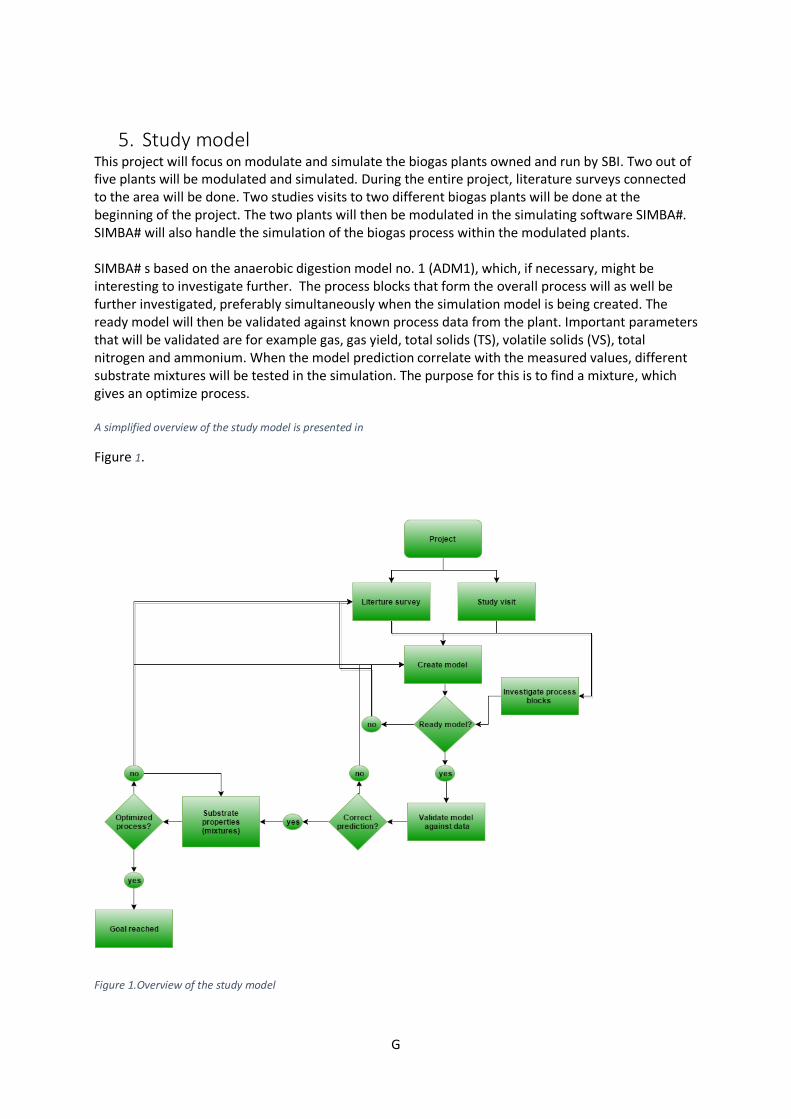
G
5. Study model This project will focus on modulate and simulate the biogas plants owned and run by SBI. Two out of five plants will be modulated and simulated. During the entire project, literature surveys connected to the area will be done. Two studies visits to two different biogas plants will be done at the beginning of the project. The two plants will then be modulated in the simulating software SIMBA#. SIMBA# will also handle the simulation of the biogas process within the modulated plants. SIMBA# s based on the anaerobic digestion model no. 1 (ADM1), which, if necessary, might be interesting to investigate further. The process blocks that form the overall process will as well be further investigated, preferably simultaneously when the simulation model is being created. The ready model will then be validated against known process data from the plant. Important parameters that will be validated are for example gas, gas yield, total solids (TS), volatile solids (VS), total nitrogen and ammonium. When the model prediction correlate with the measured values, different substrate mixtures will be tested in the simulation. The purpose for this is to find a mixture, which gives an optimize process. A simplified overview of the study model is presented in
Figure 1.
Figure 1.Overview of the study model

H
6. Milestones
Milestone number
Short description Type of deliverable
Date (week)
1 Project plan ready Report 2
2 Working simulation model ready Simulation model (SIMBA#)
6
3 Evaluated process blocks Data 8
4 Halftime report ready Report 10
5 Validated parameters Data 11
6 State optimal substrate mixture Data 17
7 Final report draft to opponent ready and sent to opponent and examiner
Report 19
8 Presentation of final report PPT 20
9 Corrected report for final approval Report 20
7. Time plan The first critical step is to obtain a simulation model that function properly. This is of high importance, since the whole project is based on modeling the biogas plants. The correlation between the simulated parameters and the measured data is as well an important step in the project, since this indicates how well the model corresponds to the reality, i.e. it tells if the model is trustworthy or not. The time plan of the project can be seen in appendix.
8. References
Akbas, H., Bilgen, B. & Turham, A. M., 2015. An integrated prediction and optimization model of biogas production system at a wastewater treatment facility. Bioresource Technolgy , Volume 196, pp. 566-576. Arnell, M., 2016. Performance Assessment of Wastewater Treatment Plants : Multi-Objective Analysis Using Plant-Wide Models. 1 ed. Lund: Lund University. Arnell, M. et al., 2016. Modelling anaerobic co-digestion in Benchmark Simulation Model No. 2: Parameter estimation, substrate characterisation and plant-wide integration.. Water Research, Volume 98, pp. 138-146. Batstone, D. J., Keller, J., Angelidaki, I. & Kal, S. V., 2002. The IWA Anaerobic Digestion Model No 1 (ADM1). Water Science and Technology, 45(10), pp. 65-73. Biernacki, P. et al., 2013. Application of Anaerobic Digestion Model No. 1 for descibing an exisiting biogas power plant. Biomass and Bioenergy, Volume 59, pp. 441-447. Fronk, K., Oguerk, M. & I, S., 2014. Modeling and simulation of biogas plants for representation of important specific parameters. Stuttgart , ifaK, pp. 1-4. Hamawand , I. & Baillie, C., 2015. Anaerobic Digestion and Biogas Potential: Simulation of Lab and Industrial-Scale Processes. Energies, Volume 8, pp. 454-474.
I
ifak , 2016. SIMBA Portal. [Online] Available at: https://simba.ifak.eu/en/content/simba-sharp-biogas [Accessed 17 January 2017]. Lindmark, J., Thorin, E., Fdhila, R. B. & Dahlquist, E., 2012. • PROBLEMS AND POSSIBILITIES WITH THE IMPLEMENTATION OF SIMULATION AND MODELING AT A BIOGAS PLANT. Suzhou, China , International Conference on Applied Energy. Lübken, M. et al., 2015. Parameter estimation and long-term process simulation of a biogasreactor operated under trace elements limitation. Applied Energy, 15 March, Volume 142, pp. 352-360. Schön, M., 2010. Numerical Modelling of Anaerobic Digestion Processes in Agricultural Biogas Plants. 1 ed. Innsbruck: Nordstedt. Swedish Biogas International, 2016. Våra anläggningar. [Online] Available at: http://www.swedishbiogas.com/index.php/sv/referensanlaeggningar [Accessed 419 01 2017]. Zaeffere, M., Gaida, D. & Bart, T., 2016. Multi-fidelity modeling and optimization of biogas plants. Applied Soft Computing, Volume 48, pp. 13-28.
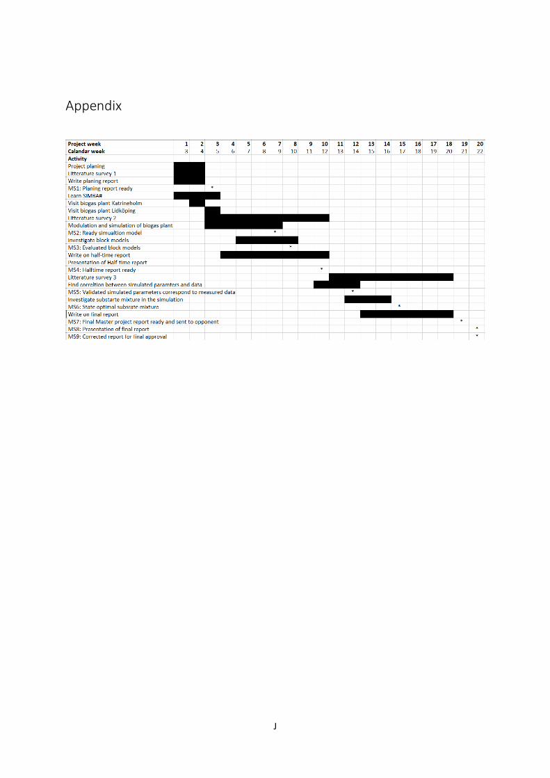
J
Appendix

K
APPENDIX B
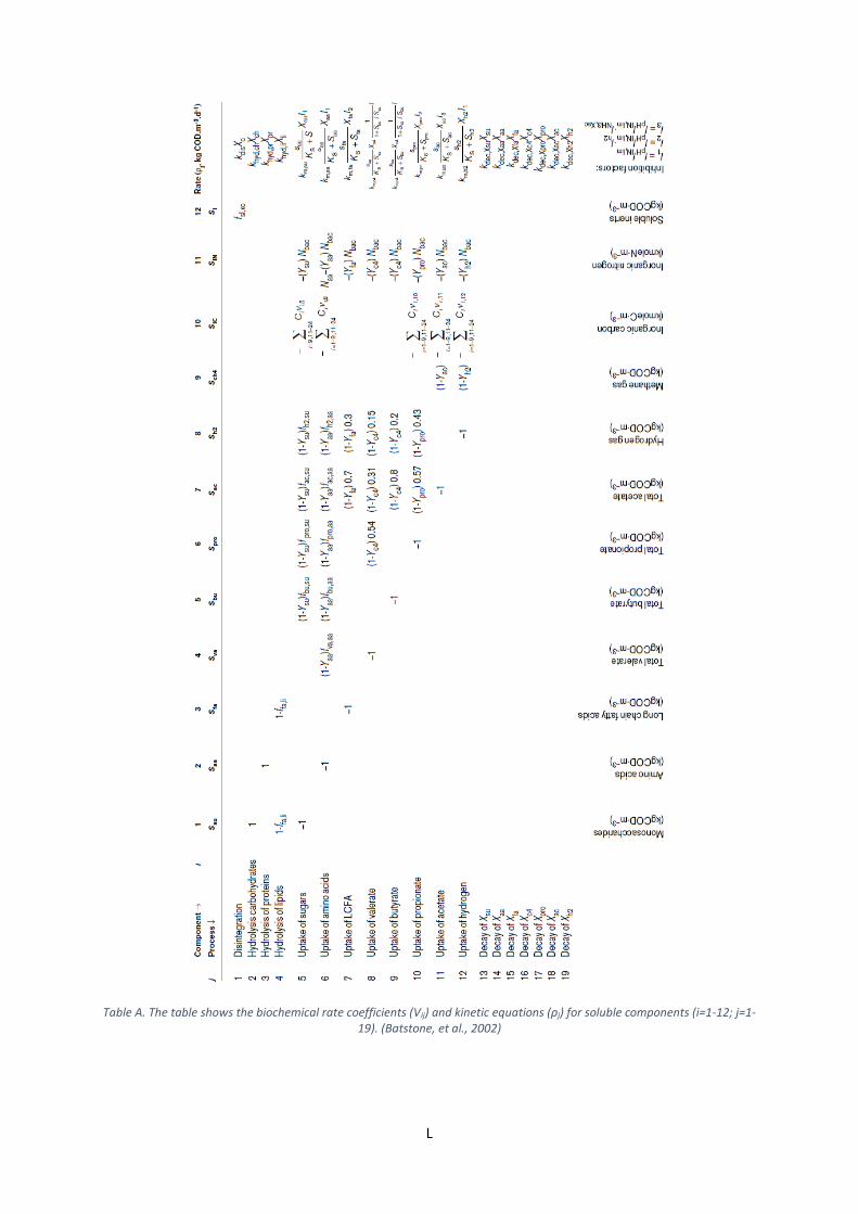
L
Table A. The table shows the biochemical rate coefficients (Vij) and kinetic equations (ρj) for soluble components (i=1-12; j=1-19). (Batstone, et al., 2002)

M
Table B. The table shows the biochemical rate coefficients (Vij) and kinetic equations (ρj) for soluble components (i=13-24; j=1-19) (Batstone, et al., 2002)
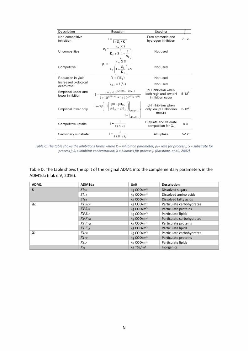
N
Table C. The table shows the inhibitions forms where Ki = inhibition parameter; ρj = rate for process j; S = substrate for process j; SI = inhibitor concentration; X = biomass for process j. (Batstone, et al., 2002)
Table D. The table shows the split of the original ADM1 into the complementary parameters in the
ADM1da (ifak e.V, 2016).
ADM1 ADM1da Unit Description
Si 𝑆𝐼𝑆𝑈 kg COD/m3 Dissolved sugars
𝑆𝐼𝐴𝐴 kg COD/m3 Dissolved amino acids
𝑆𝐼𝐹𝐴 kg COD/m3 Dissolved fatty acids
𝑋𝐶 𝑋𝑃𝑆𝐶𝐻 kg COD/m3 Particulate carbohydrates
𝑋𝑃𝑆𝑃𝑅 kg COD/m3 Particulate proteins
𝑋𝑃𝑆𝐿𝐼 kg COD/m3 Particulate lipids
𝑋𝑃𝐹𝐶𝐻 kg COD/m3 Particulate carbohydrates
𝑋𝑃𝐹𝑃𝑅 kg COD/m3 Particulate proteins
𝑋𝑃𝐹𝐿𝐼 kg COD/m3 Particulate lipids
𝑋𝐼 𝑋𝐼𝐶𝐻 kg COD/m3 Particulate carbohydrates
𝑋𝐼𝑃𝑅 kg COD/m3 Particulate proteins
𝑋𝐼𝐿𝐼 kg COD/m3 Particulate lipids
𝑋𝑀 kg TSS/m3 Inorganics

O
APPENDIX C
Lidköping: Bio-fertilizers
Figure A. The figure show how well the simulation (blue) correlates with the measured NH4-N concentration (green) in the fertilizer tank of the Lidköping model. As one can be seen in the figure, the simulation has an overshoot at both the beginning and the end of the simulation, leading to badly correlated prediction.
Figure B. The figure show how well the simulation (blue) correlates with the measure N-total concentration (red) in the fertilizer tank of the Lidköping model. As can be seen in the figure, the simulation has an overshoot for all data point, which means that the prediction misses out and does not correlate with measured data.
0
0,5
1
1,5
2
2,5
3
0
10
20
30
40
50
60
70
80
90
10
0
11
0
12
0
13
0
14
0
15
0
16
0
17
0
18
0
19
0
20
0
21
0
22
0
23
0
24
0
25
0
26
0
27
0
28
0
29
0
30
0
31
0
32
0
33
0
34
0
35
0
36
0
[kg
N/m
3 ]
Time [days]
NH4-N simulated NH4-N measured
0
1
2
3
4
5
6
7
0
10
20
30
40
50
60
70
80
90
10
0
11
0
12
0
13
0
14
0
15
0
16
0
17
0
18
0
19
0
20
0
21
0
22
0
23
0
24
0
25
0
26
0
27
0
28
0
29
0
30
0
31
0
32
0
33
0
34
0
35
0
36
0
[kg
N/m
3]
Time [days]
N-total simulated N-total measured
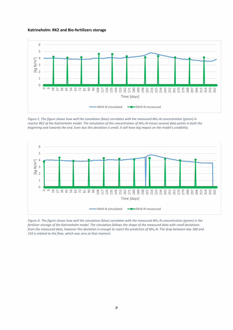
P
Katrineholm: RK2 and Bio-fertilizers storage
.
Figure C. The figure shows how well the simulation (blue) correlates with the measured NH4-N concentration (green) in reactor RK2 of the Katrineholm model. The simulation of the concentration of NH4-N misses several data points in both the beginning and towards the end. Even due this deviation is small, it will have big impact on the model’s credibility.
Figure D. The figure shows how well the simulation (blue) correlates with the measured NH4-N concentration (green) in the fertilizer storage of the Katrineholm model. The simulation follows the shape of the measured data with small deviations from the measured data, however this deviation is enough to reject the prediction of NH4-N. The drop between day 180 and 210 is related to the flow, which was zero at that moment.
0
1
2
3
4
5
60 9
18
27
36
45
54
63
72
81
90
99
10
8
11
7
12
6
13
5
14
4
15
3
16
2
17
1
18
0
18
9
19
8
20
7
21
6
22
5
23
4
24
3
25
2
26
1
27
0
27
9
28
8
29
7
30
6
31
5
32
4
33
3
34
2
[kg
N/m
3 ]
Time [days]
NH4-N simulated NH4-N measured
0
1
2
3
4
5
6
0 9
18
27
36
45
54
63
72
81
90
99
10
8
11
7
12
6
13
5
14
4
15
3
16
2
17
1
18
0
18
9
19
8
20
7
21
6
22
5
23
4
24
3
25
2
26
1
27
0
27
9
28
8
29
7
30
6
31
5
32
4
33
3
34
2
[kg
N/m
3 ]
Time [days]
NH4-N simulated NH4-N measured

Q
APPENDIX D
Economical calculations
Transportation costs
The distance for the transportations of both incoming and outgoing manure and bio-fertilizers are
estimated to not farther than 25 km from the plant. This gives a transportation price of 17.63 kr per
m3. The same assumption and price is used for both plants.
Lidköping
The example below is calculated for the case when 6000 tons/year of food residues is used in the
production. The other cases are calculated in the same way but with other volumes of water and
manure.
Table E. The table shows the calculation cost for the transportation to and out of Lidköping.
Total swine manure
[m3/day]
Total water
[m3/day]
Transportation cost in
[kr/day]
Sludge out
[m3/day]
Transportation cost of
bio-fertilizers [kr/day]
Total transportation
cost [kr/day]
Non 41.002 0 41.002*17.63 = 722.9
343.7 343.7*17.63 = 6059.4 6782.3
Water ABP 41.002 38 41.002*17.63 = 1392.8
382.2 382.2*17.63 = 6738.2 8131.0
Swine manure ABP
116.022 0 116.022*17.63 = 2045.1
418.8 418.8*17.63 = 7383.4 9428.6
Water All 41.002 290 41.002*17.63 = 722.9
490.2 490.2*17.63 =8642.2 9365.1
Swine manure All
331.002 0 331.002*17.63 = 11172.1
633.7 633.7*17.63 = 11172.1 17007.7
Katrineholm
Table F. The table shows the calculation cost for the transportation to and out of Katrineholm.
Total swine manure [m3/day]
Chicken manure
[ton/day]
Transportation cost in
[kr/day]
sludge out
[m3/day]
Transportation cost of
bio-fertilizers [kr/day]
Total transportation
costs [kr/day]
Open system 65.48 0 65.48*17.63 =1154.74
202.73 202.73*17.63 =3575.144
4729.89
Recirculated system 6.16 0 6.16*17.63 = 108.6
143.27 143.27*17.63 = 2525.8
2634.4
Recirculated system with added chicken manure
6.16 2.4 (6.16+2.4)*17.63 = 150.9
146.72 146.72*17.63 = 2589.7
2740.6