modeling and simulation of ice body/ship structure

Naval Surface Warfare Center Carderock Division West Bethesda, MD 20817-5700

Distribution Statement A. Approved for public release. Distribution is unlimited.

NSWCCD-65-TR–2019/08 February 2020

Platform Integrity Department

Technical Report

Modeling and Simulation of Ice Body/Ship Structure Collision with Inelastic Structural Deformation Including Rupture and Tearing

by

Douglas E. Lesar

NS

WC

CD

-65-T

R–2

01

9/0

8

Mo

de

lin

g a

nd

Sim

ula

tio

n o

f Ic

e B

od

y/S

hip

Str

uctu

re C

ollis

ion

wit

h In

ela

sti

c S

tru

ctu

ral D

efo

rma

tio

n

Inclu

din

g R

up

ture

an

d T

ea

rin

g

Naval Surface Warfare Center Carderock Division West Bethesda, MD 20817-5700

Distribution Statement A. Approved for public release. Distribution is

unlimited.

NSWCCD-65-TR–2019/08 February 2020

Platform Integrity Department Technical Report

Modeling and Simulation of Ice Body/Ship Structure Collision with Inelastic Structural Deformation

Including Rupture and Tearing by

Douglas E. Lesar

REPORT DOCUMENTATION PAGE Form Approved

OMB No. 0704-0188 Public reporting burden for this collection of information is estimated to average 1 hour per response, including the time for reviewing instructions, searching existing data sources, gathering and maintaining the data needed, and completing and reviewing this collection of information. Send comments regarding this burden estimate or any other aspect of this collection of information, including suggestions for reducing this burden to Department of Defense, Washington Headquarters Services, Directorate for Information Operations and Reports (0704-0188), 1215 Jefferson Davis Highway, Suite 1204, Arlington, VA 22202-4302. Respondents should be aware that notwithstanding any other provision of law, no person shall be subject to any penalty for failing to comply with a collection of information if it does not display a currently valid OMB control number. PLEASE DO NOT RETURN YOUR FORM TO THE ABOVE ADDRESS.

1. REPORT DATE (DD-MM-YYYY)

05-Feb-2020

2. REPORT TYPE

Final

3. DATES COVERED (From - To)

-

4. TITLE AND SUBTITLE

Modeling and Simulation of Ice Body/Ship Structure Collision

with Inelastic Structural Deformation Including Rupture and

Tearing

5a. CONTRACT NUMBER

N0001419WX00399

5b. GRANT NUMBER

5c. PROGRAM ELEMENT NUMBER

0602123N

6. AUTHOR(S)

Douglas E. Lesar

5d. PROJECT NUMBER

5e. TASK NUMBER

5f. WORK UNIT NUMBER

7. PERFORMING ORGANIZATION NAME(S) AND ADDRESS(ES) AND ADDRESS(ES) 8. PERFORMING ORGANIZATION REPORT NUMBER

NSWCCD-65-TR–2019/08

Naval Surface Warfare Center

Carderock Division

9500 Macarthur Boulevard

West Bethesda, MD 20817-5700

9. SPONSORING / MONITORING AGENCY NAME(S) AND ADDRESS(ES) 10. SPONSOR/MONITOR’S ACRONYM(S)

Attn: ONR 331

Chief of Naval Research

One Liberty Center

875 N. Randolph Street, Suite

1425

Arlington, VA 22203-1995

11. SPONSOR/MONITOR’S REPORTNUMBER(S)

12. DISTRIBUTION / AVAILABILITY STATEMENT

Distribution Statement A. Approved for public release. Distribution is unlimited.

13. SUPPLEMENTARY NOTES

14. ABSTRACT

This report documents numerical simulations of rigid and nonrigid ice body impact on notional

naval surface ship structure. The impacting body first indents the hull structure a prescribed

amount and then slides along the hull in scoring fashion across several hull frames. Initial

analyses assume a rigid indenter, and subsequent analyses utilize indenter material models used in

prior analyses to represent localized ice crushing. The ice material models do not capture

spalling, flaking, or ice rubble confinement. These simulations allow permanent set deformation in

the hull structure, as well as structural rupture and tearing according to dependence of failure

strain on stress triaxiality under plane-stress assumptions. The simulations benefit from mesh-

dependence-mitigating practices developed by other U.S. Navy analysts. These studies demonstrate

both simulation capability and engineering insights. Although structural permanent set and tearing

damage is greatest when the indenting-and-scoring body is rigid and damage decreases as ice

rigidity decreases, the peak load does not parallel this trend. Since structural capacity falls

from the undamaged structure level once tearing begins, and since tearing failure commences early

in the rigid-indenter event, the peak load developed by a less-than-rigid indenter is greater than

that induced by a rigid indenter. Another notable finding is that a more-compliant indenter

develops high load at a stiff bulkhead location before tearing occurs. This result indicates that

structural “hard spots” are likely tearing initiation locations and illustrate interaction between

local structure compliance and assumed ice strength in rupture and tearing prediction.

15. SUBJECT TERMS

Ship Structures, Structural Damage, Structural Failure Modes, Finite Element Analysis

16. SECURITY CLASSIFICATION OF: 17. LIMITATIONOF ABSTRACT

SAR

18. NUMBEROF PAGES

80

19a. NAME OF RESPONSIBLE PERSON

Mr. Douglas E. Lesar

a. REPORT

UNCLASSIFIED

b. ABSTRACT

UNCLASSIFIED

c. THIS PAGE

UNCLASSIFIED

19b. TELEPHONE NUMBER (include area

code)

(301)227-1803

iii Standard Form 298 (Rev. 8-98)

Prescribed by ANSI Std. Z39.18

iv

This page intentionally left blank.

NSWCCD-65-TR-2019/08

v

Contents

Page Contents ...........................................................................................................................................v

Figures............................................................................................................................................ vi Tables ............................................................................................................................................ vii Preface.......................................................................................................................................... viii Acknowledgments........................................................................................................................ viii 1. Summary .....................................................................................................................................1

2. Introduction .................................................................................................................................2

3. Methods, Assumptions, and Procedures .....................................................................................4 3.1 Analysis Software ............................................................................................................4 3.2 Structural Scantlings ........................................................................................................4 3.3 Hull Structure Modeling ..................................................................................................8 3.4 Hull Material Modeling .................................................................................................10 3.5 Rigid and Compliant Indenter Modeling .......................................................................16 3.6 Collision Kinematics......................................................................................................20 3.7 Simulation Assumptions ................................................................................................20 3.8 Simulation Hardware and Code Versions ......................................................................22

4. Results and Discussion .............................................................................................................23 4.1 Rigid Indenter Simulations without Structural Fracture Occurrence ............................23

4.1.1 Comparison of MAT24 with MAT224 ..............................................................24 4.1.2 MAT224 Parameter Definition Checks .............................................................26

4.2 Rigid Indenter Simulations with Reduced Structural Failure Strains ............................27 4.2.1 LS-DYNA Code Version Check and Failopt Parameter

Influence .............................................................................................................28 4.2.2 Eroding Contact Surface Evaluation ..................................................................31

4.3 Rigid and Glacial Ice Indenter Simulations with Realistic Structural Failure Strains and Doubled Initial Penetration...........................................................35 4.3.1 Initial Glacial Ice Indenter Simulations .............................................................36 4.3.2 Additional Glacial Ice Indenter Simulations......................................................39

4.4 Compliant Ice Indenter Simulations with Doubled Initial Penetration ..........................42 4.4.1 Compliant Ice Indenter Simulations without Contact Friction ..........................43 4.4.2 Compliant Ice Indenter Simulations with Contact Friction ...............................47

5. Conclusions ...............................................................................................................................53

6. Recommendations .....................................................................................................................56

7. References .................................................................................................................................58


vi

Appendix A Development of DH36 Steel Failure-Strain Curve as a Function of Stress Triaxiality for Plane-Stress Conditions ......................................................................61

Appendix B Development of Ice/Steel Friction Coefficients from Field Test Data .....................65

Figures

Page Figure 1. H3000 Section Chosen for Representative Structural Modeling ....................................5 Figure 2. H3000 Structural Scantlings ............................................................................................6 Figure 3. LS-DYNA Structural Idealization of H3000 Bow Region Structure ..............................9 Figure 4. Nodal Constraints Applied to H3000 FEM .....................................................................9 Figure 5. FE Mesh of H3000 Moving Indenter ............................................................................16 Figure 6. Initial Indenter Position Outboard of a H3000 Frame Midbay .....................................17 Figure 7. Comparison of Volumetric-Strain-versus-Yield-Stress Curves for

Various LS-DYNA MAT63 Ice Models ..........................................................................19 Figure 8. Imposed Indenter Motions .............................................................................................20 Figure 9. Resultant Contact Force Histories for Rate-Independent and Rate-

Dependent DH36 Steel Properties ....................................................................................25 Figure 10. Final Effective-Plastic-Strain Contours for Rate-Independent and

Rate-Dependent DH36 Steel Properties ...........................................................................26 Figure 11. Resultant Contact Force Histories for Two MAT224 Failure Options .......................29 Figure 12. Final Effective-Plastic-Strain Contours and Tearing Damages for Two

MAT224 Failure Options .................................................................................................30 Figure 13. Resultant Contact Force Histories for Noneroding and Eroding

Contacts ............................................................................................................................32 Figure 14. Final Effective-Plastic-Strain Contours and Tearing Damages for

Noneroding and Eroding Contacts ...................................................................................32 Figure 15. Resultant Contact Force Histories for Eroding Contact Options ................................33 Figure 16. Final Effective-Plastic-Strain Contours and Tearing Damages for

Eroding Contact Options ..................................................................................................34 Figure 17. Resultant Contact Force Histories for Rigid and MAT63 Indenters ...........................38 Figure 18. Final Effective-Plastic-Strain Contours and Tearing Damages for

Rigid and MAT63 Indenters .............................................................................................38 Figure 19. Resultant Contact Force Histories with MAT63 Indenters for

Alternative Contact Surface and Hourglass Control Assumptions ..................................40 Figure 20. Final Effective-Plastic-Strain Contours and Tearing Damages with

MAT63 Indenters for Alternative Contact Surface and Hourglass Control Assumptions .....................................................................................................................41

Figure 21. Resultant Contact Force Histories for Rigid, MAT63, and MAT3 Compliant Indenters, Zero Interface Friction ...................................................................45

Figure 22. Final Effective-Plastic-Strain Contours and Tearing Damages for Rigid, MAT63, and MAT3 Compliant Indenters, Zero Interface Friction ......................46

Figure 23. Examples of Rigid Indenter/Structure Contact Areas and Pressures ..........................49


vii

Figure 24. Examples of Compliant Indenter/Structure Contact Areas and Pressures ...........................................................................................................................50

Figure A1. True-Stress-versus-True-Strain Curves for DH36 Steel for Two Strain Rates .................................................................................................................................62

Figure A2. Major Strain at Failure versus Minor Strain, DH36 Steel ..........................................63 Figure A3. Effective Plastic Failure Strain versus Stress Triaxiality, DH36 Steel.......................64 Figure B1. Ice/Structure Friction Coefficient Presumed in LS-DYNA Simulations

with Contact Friction ........................................................................................................66

Tables

Page Table 1. H3000 Plate and Stiffening Frame Properties ..................................................................5 Table 2. Original H3000 Structural Material Properties ...............................................................10 Table 3. DH36 Basic Material Properties .....................................................................................12 Table 4. Effective True Stress as Function of True Strain for DH36 at 0.001 s-1.........................13 Table 5. Strain Rate Scale Factors on Effective Stress for DH36 ................................................13 Table 6. Failure Strain as a Function of Stress Triaxiality for DH36 ...........................................15 Table 7. LS-DYNA MAT63 Parameters for Ice Crushing, 2007 and 2017b

Parameter Sets ..................................................................................................................18 Table 8. LS-DYNA MAT3 Parameters for Ice Crushing .............................................................19 Table 9. Particulars of LS-DYNA Group 1 Analyses...................................................................24 Table 10. Peak Contact Forces and Inelastic Strains for LS-DYNA Group 1

Analyses, MAT24/MAT224 Correlation .........................................................................25 Table 11. Peak Contact Forces and Inelastic Strains for LS-DYNA Group 1

Analyses, MAT224 Parameter Definition Checks ...........................................................27 Table 12. Particulars of LS-DYNA Group 2 Analyses.................................................................28 Table 13. Peak Contact Forces and Inelastic Strains for LS-DYNA Group 2

Analyses, MAT224 Failure Criteria Checks ....................................................................29 Table 14. Peak Contact Forces and Inelastic Strains for LS-DYNA Group 2

Analyses, Eroding Contact Evaluations ...........................................................................31 Table 15. Particulars of LS-DYNA Group 3 Analyses.................................................................36 Table 16. Peak Contact Forces and Failure Results for LS-DYNA Group 3

Analyses, Initial MAT63 Indenter Modeling Attempts ...................................................37 Table 17. Peak Contact Forces and Failure Results for LS-DYNA Group 3

Analyses, Additional MAT63 Indenter Modeling Attempts ............................................40 Table 18. Particulars of LS-DYNA Group 4 Analyses.................................................................43 Table 19. Peak Contact Forces and Inelastic Strains for LS-DYNA Group 4

Analyses, Frictionless Contact .........................................................................................44 Table 20. Peak Contact Forces and Inelastic Strains for LS-DYNA Group 4

Analyses, Contact with and without Ice/Steel Friction ....................................................48 Table 21. Summary of Key Results for the Highest-Quality Indenter/Hull

Structure Damage Simulations .........................................................................................54 Table B1. Measured Kinetic Friction Coefficient Data for Ice/Corroded Steel

Sliding...............................................................................................................................66


viii

Preface

The Structures and Composites Division (Code 65) of the Platform Integrity Department at Naval Surface Warfare Center, Carderock Division (NSWCCD) performed the work described in this report during the period from October 2018 to March 2019. Office of Naval Research (ONR), Sea Warfare and Weapons Department, Ship Systems and Engineering Research Division (ONR 331) provided funding to support this effort. NSWCCD performed the work under funding document N0001419WX00399, program element 0602123N.

ONR requested NSWCCD to develop capabilities, using advanced computational structural dynamics modeling and simulation (M&S) methods, for simulation of response and failure analysis of non-ice-classed ship structures subjected to collision with sea ice in the marginal ice zone. Two motivations impel this work: (1) a need to advance U.S. Navy’s (USN) ability to quantify the risk associated with operating surface combatants in ice-infested polar waters, and (2) a need to develop surface combatant operating guidance minimizing risk to hull structural integrity during polar-region operations. This document is a continuation of a prior NSWCCD report (Lesar, 2019), which documents structure and ice collision simulations considering permanent set deformation damage in the structure. This report concerns follow-on efforts considering structural rupture and tearing damage.

Acknowledgments

The author thanks Dr. Paul Hess III of ONR for, starting in 2010, having the foresight to restore USN science and technology (S&T) attention to this increasingly important technical area. The author also extends thanks to Dr. Ken Nahshon (NSWCCD 664), who provided key advice and guidance concerning cost-effective and engineering-level accurate numerical modeling of fracture and tearing behaviors in thin shell structures.The hardware and software resources of the Department of Defense (DoD) High Performance Computing Centers were essential to timely completion of the dozens of simulations performed in the course of this effort.


1

1. Summary

This report documents numerical simulations of rigid and nonrigid ice body impact on notional naval surface ship structure. The impacting body first indents the hull structure a prescribed amount and then slides along the hull in scoring fashion across several hull frames. Initial analyses assume a rigid indenter, and subsequent analyses utilize indenter material models used in prior analyses to represent localized ice crushing. The ice material models do not capture spalling, flaking, or ice rubble confinement. These simulations allow permanent set deformation in the hull structure, as well as structural rupture and tearing according to dependence of failure strain on stress triaxiality under plane-stress assumptions. The simulations benefit from mesh-dependence-mitigating practices developed by other U.S. Navy analysts. These studies demonstrate both simulation capability and engineering insights. Although structural permanent set and tearing damage is greatest when the indenting-and-scoring body is rigid and damage decreases as ice rigidity decreases, the peak load does not parallel this trend. Since structural capacity falls from the undamaged structure level once tearing begins, and since tearing failure commences early in the rigid-indenter event, the peak load developed by a less-than-rigid indenter is greater than that induced by a rigid indenter. Another notable finding is that a more-compliant indenter develops high load at a stiff bulkhead location before tearing occurrs. This result indicates that structural “hard spots” are likely tearing initiation locations and illustrate interaction between local structure compliance and assumed ice strength in rupture and tearing prediction.


2

2. Introduction

Existing semiempirical toolsets are adequate for design and assessment of ice-classed hull structures for ships that are completely dedicated to icebreaking or must routinely operate in ice-infested waters. However, these toolsets assume robust hull structural configurations incompatible with structural weight and cost constraints of warship design. This report focuses on numerical modeling and simulation (M&S) methods accounting for ice crushing, ice fracture, large hull structure deformation, plasticity, tearing, and rupture to investigate the shared-energy collision and damage physics phenomena that are likely present when non-ice-classed hull structure collides with floe or glacial ice.

The first NSWCCD report issued for this project (Lesar, 2017) provided a survey and assessment of numerical M&S methods used in past ice-structure interaction studies and more novel methods that have potential for this technical area. It was found the that finite element (FE) method had been the most widely applied in both research and engineering, and though the complexity of material response and complex failure behavior of ice has prevented development of an all-encompassing first-principles material model for ice, classical plasticity models could be exploited and tuned for engineering-level ice modeling purposes. Alternative modeling approaches, such as smoothed-particle hydrodynamics (SPH), the discrete element method (DEM), and element-free Galerkin (EFG), have been considered by ice mechanics researchers but are not yet mature enough for engineering application.

This earlier report (Lesar, 2017) also documents a series of FE-based ice beam flexural fracture simulations, which, through comparisons with a limited experimental data set, validated usage of a properly tuned inelastic material model in the LS-DYNA explicit nonlinear dynamics analysis code (Livermore Software Technology Corporation (LSTC), 2017) for modeling this mode of ice failure. This model was combined with an inelastic LS-DYNA material model for simulating ice crushing in the immediate ice/structure contact zone in an analysis series demonstrating ice slab fracture distant from the crushing zone. In these computational experiments, a bimaterial ice slab was loaded by a moving rigid wall sloped at a 10° angle with respect to the vertical and an 80° angle with respect to the impacted slab. Physically plausible radial and circumferential crack patterns developed, though the LS-DYNA element deletion process may not have been optimally managed. Structure/ice contact surface friction assumptions strongly influenced the ice slab failure process.

A follow-on effort replaced the inclined rigid wall with LS-DYNA-modeled non-ice-reinforced surface ship hull structure, including elastic-plastic structural material response as well as ice slab crushing and flexural fracture (Lesar, 2019). In this study, the notional local surface ship hull structural models used by Dolny, Daley, Quinton, and Daley (2016, 2017a) were loaded on longitudinal or transverse stiffeners by ice slabs ranging in thickness from 0.14 m to 0.35 m. Better-managed LS-DYNA element deletion criteria produced cleaner ice flexural fracture patterns, and inelastic deformation levels in the structure were tracked and compared for analysis variations with ice fracture either allowed or prevented. Most analyses considered an almost static ice/structure approach rate (somewhat more than 1 kn relative speed), consistent with the analyses by Dolny et al. (2016, 2017a). A few additional simulations assumed a relative speed of 4 kn. Baseline analyses did not allow fracture anywhere in the ice, and parallel


3

simulations allowed fracture in the great bulk of the ice beyond a small crushing-only zone near the structural contact area. In addition to frictionless cases, analyses with contact surface friction included a constant static and dynamic coefficient of 0.10, as presumed by Dolny et al. (2016, 2017a).

Even for these quite-thin slabs and with ice floe motion constrained by a fixed far-field boundary, ice flexural fracture did not consistently limit the peak loads imparted to the structure. Effectively, the non-ice-classed structure was the “weak link” in the coupled ice-structure system. The effect of ice/structure contact friction was more significant, with peak loads and inelastic structural damage in nonzero-friction cases consistently increased above companion simulations with zero interface friction.

A key engineering conclusion by Lesar (2019) is that when considering ice/structure interaction for relatively wall-sided non-ice-classed and nonicebreaking hull forms, a “flexural limit” that limits level ice and ice floe loading at lower ice thicknesses cannot be relied upon. As a result, loadings presuming that no flexural fracture occurs are not likely to be overly conservative for structural risk assessment or design efforts.

The work documented by Lesar (2017, 2019) focused on thin-ice impact scenarios where loading, limited by low relative ice/structure velocity and low ice body mass and stiffness, confines structural damage to permanent set deformation and is insufficient to attain structural rupture and tearing. A chief goal of the current effort is to exercise and demonstrate a capability for modeling rupture and tearing damage in ice-loaded hull structure. The approach to achieve this objective is to carry out LS-DYNA ice impact analyses of the same hull structural configuration used by Lesar (2019) with rupture and tearing damage mechanisms enabled in the structural material modeling.

This report systematically documents extension of M&S competence and experience to account of these more severe structural damage mechanisms, including consideration of indenter compliance (rigid body versus deformable ice). This work is carried out by via the modeling methods and assumptions delineated in section 3, systematically conducting several groups of simmulations:

• Rigid Indenter Simulations without Structural Fracture Occurrence; evaluating moving-ice-load simulations but substituting HY80 steel with lower-strength DH36.

• Rigid Indenter Simulations with Reduced Structural Failure Strains; accomplishing hull steel failure by presuming artificially lower DH36 failure strains.

• Rigid and Glacial Ice Indenter Simulations with Realistic Structural Failure Strains and Doubled Initial Penetration; accomplishing hull shell rupture and tearing by increasing indenter penetration.

• Compliant Ice Indenter Simulations with Doubled Initial Penetration; an analysis series considering ice indenters with various crushing compliance levels.

The results of these simulations and findings are detailed in section 4; overall summaries are listed in the conclusion detailed in section 5, as well as a section 6 which provides detailed recommendations for future work in this challenging area.


4

3. Methods, Assumptions, and Procedures

This major section describes the ship structure analyzed, its numerical discretization and material modeling assumptions, the modeled indenter and its material modeling, kinematic assumptions of the structure and indenter interaction, and numerical modeling software and computation hardware.

3.1 Analysis Software LS-DYNA is a general-purpose, three-dimensional (3D), nonlinear finite element analysis

(FEA) code, developed and maintained by LSTC (2015). This code addresses high-rate dynamic problems in which large deflections, complex evolving mechanical contacts, nonlinear material behavior, and material failure are predominant. It addresses static and dynamic problems involving solids and structures, possesses adjunct fluid domain modeling capabilities, and enables treatment of various fluid-structure interactions. It uses explicit time-integration methods, but it can also carry out implicit solution of low-rate or static problems. Several LS-DYNA applications to problems in the ice mechanics and ice/structure impact areas may be cited (Das, Polić, Ehlers, & Amdahl, 2014; Gagnon & Derradji-Aouet, 2006; Gagnon & Wang, 2012; Kim, 2014; Kim, Storheim, Amdahl, Løset, & von Bock und Polach, 2016; Liu, Amdahl, & Løset, 2011a; Sazidy, 2015).

3.2 Structural Scantlings Numerous LS-DYNA finite element models (FEMs), developed under contract to ONR by

a team composed of the American Bureau of Shipping (ABS) and Memorial University (MUN), were made available to the USN (Dolny et al., 2016, 2017a). ABS and MUN included a detailed local structural idealization of a generic Naval surface ship based on the notional “Hull 3000” (H3000) hull form. NSWCCD developed the hull plating, longitudinal and transverse stiffeners, decks, and bulkheads in the resulting FEM, based on ship structural design practices.

Dolny et al. used LS-DYNA idealizations of H3000 (with case-dependent FE model extent adaptations) in five ice/structure impact studies:

a. Development of structural-deformation-based adjustments to the spreadsheet-based ice loading computation tool DDePs (Direct Design of Polar Ships, developed by BMT Fleet Technology and the American Bureau of Shipping)1, which normally presumes a rigid structure (Dolny et al., 2016)

b. Analysis of structural response to stationary, increasing patch loads (Dolny et al., 2016) c. Analysis of structural response to a moving rigid indenter (Dolny et al., 2017a) d. Analysis of structural response to moving and spatially-varying (“4D”) patch loads

based on ice loading field measurements reported by Daley, St. John, Brown, and Glen (1990) for USCGC Polar Sea (WAGB 11) (Dolny et .al., 2017a)

1 There is no one report documenting DDePS, but Dolny et al. (2016) list several contributing references.


5

e. Analysis of structural response to impact by crushable ice slabs (Dolny et al., 2017a) The effort documented by Lesar (2019) used one of the Dolny et al. LS-DYNA H3000

idealizations to consider the effect of ice flexural fracture on structural permanent set damage. This work was an extension of the Dolny et al. study (e), which considered only ice slab crushing behavior. The present report concerns two extensions of study (c) by Dolny et al.: (1) allowance of rupture and tearing damage in the hull structure, and (2) replacement of the rigid indenter with a compliant indenter assigned with engineering-level ice crushing material models used by ice-loaded structure engineering practitioners.

Figure 1 is a nominal lines drawing of the H3000 hull form, and the scantlings of the local structural idealization of the H3000 are based on those for the hull section located 18.3 m aft of the forward perpendicular.

Figure 1. H3000 Section Chosen for Representative Structural Modeling

Table 1 lists, and Figure 2 illustrates, the notional scantlings of this representative structure located in the bow region of the ship.

Table 1. H3000 Plate and Stiffening Frame Properties

Components Plate Thicknesses (mm) Upper and Lower Hull Shell 10.0

Middle Hull Shell and Deck 1 8.0 Other Decks, Bulkheads, and

Floors 6.0

Parameters Frame Type and Dimensions (mm)

Longitudinal Transverse Frame Span 2032 2500

Frame Spacing 685 2032 Web Height 145 390

Web Thickness 5.0 6.0 Flange Width 100 140

Flange Thickness 5.0 9.0


6

NOTE: structural material = DH36 steel

(a) Sections Between Transverse Frames

NOTE: structural material = DH36 steel

(b) Sections at Web Frames and Bulkheads Figure 2. H3000 Structural Scantlings


7

(c) Longitudinal Framing Detail

(d) Framing Arrangements on Hull Shell

Figure 2. H3000 Structural Scantlings (cont’d)

10 mm shell thickness




8

The following subsections present assumptions and details in the LS-DYNA ship hull structural model based on the scantlings of Table 1 and Figure 2,and rigid or compliant indenter FEMs.

3.3 Hull Structure Modeling The LS-DYNA discretization of H3000 hull structure used in the present studies, based on

the plate and stiffener scantlings shown in Figure 2, spans six transverse hull frame spacings and includes a central transverse bulkhead. The discretization extends from the keel to the main deck level and includes deep floors, first deck (tank top), second deck, third deck, main deck, transverse tee frames, and longitudinal tee stiffeners on both side shell and decks. Bulkhead stiffeners and brackets are also included. Only one (port or starboard) side of the hull is modeled, and waterline angles of the hull form are not considered, i.e., the sectional areas of each frame location are the same, and transverse dimensions from centerline do not vary fore and aft. Figure 3 illustrates the LS-DYNA idealization, based on the ABS/MUN-developed FEM designated with LS-DYNA input file name large_hull_mesh_10cm_refined2.k, used in LS-DYNA runs H_421 and H_422, as reported by Dolny et al. (2017a, section 3.4). The left-hand view of Figure 3 shows plating and stiffener outlines, while the right-hand view displays the shell element mesh. The model is composed of 17 parts, distinguishing between side shell, longitudinal stiffener, transverse frame webs and flanges, deep floors, bulkheads, and decks. The mesh is composed of 68892 nodes, 69215 shell elements, and zero beam elements, with all stiffeners discretized as shells.2 The discretization on the hull plating follows, roughly, 10-cm lateral shell element dimensions in the majority of the model, with roughly 5-cm element sizes in a more densely meshed zone flanking the design waterline, the region most likely to suffer sliding impact with a floating ice body. These element sizes followed from material failure modeling considerations later discussed in section 3.4.

2 The ABS/MUN team has provided structural modeling guidelines for hull structure/ice collision modeling

(Quinton, Daley, Gagnon, & Colbourne, 2017).


9

Figure 3. LS-DYNA Structural Idealization of H3000 Bow Region Structure

This model is twice the length of that used in previous studies by Lesar (2019), since damage propagation by indenter movement along a greater length of the hull, including traversal over a stiff transverse bulkhead as well as typical transverse frames, is of interest. Unlike the smaller FEM used previously, this model lacks bulkheads at the forward and aft ends. These were necessary in those prior analyses to provide stable lateral motion of the hull section into nearby ice slabs. In this case, the forward- and aft-most extremities of the FEM are held fixed, and stabilizing bulkheads are not needed. Figure 4 shows, with tick marks, constrained structural nodes on the six-frame H3000 FEM periphery. All nodes on the port-starboard symmetry plane are constrained as fixed in addition to those on the forward and aft ends.

Figure 4. Nodal Constraints Applied to H3000 FEM


10

3.4 Hull Material Modeling In the original ABS/MUN studies (Dolny et al., 2016, 2017a) and work by Lesar (2019),

the hull material was specified as HY-80 steel. Table 2 lists the assumed HY-80 material properties, in both Imperial and meter-kilogram-second (MKS) units, for the LS-DYNA material model used in these analyses, the bilinear elastic-plastic strain-hardening material MAT_PLASTIC_KINEMATIC (MAT3).

Table 2. Original H3000 Structural Material Properties

HY-80 Material Property Value in U.S. (Imperial) Units Value in SI (MKS) Units

Mass Density 0.283 lbf/in3 7833 kg/m3

Elastic Modulus 29.6 Msi 204 GPa

Poisson’s Ratio 0.3 0.3

Yield Strength 80 ksi 551.6 MPa

Ultimate Tensile Strength 100 ksi 689.5 MPa

Ultimate Tensile Strain 0.2 0.2

Bilinear Elastic-Plastic-Kinematic Hardening Model Parameters*

Tangent Modulus* 101 ksi 0.7 GPa

Hardening Parameter 0.0 0.0 Note: * Tangent modulus derives from yield strength, ultimate tensile strength, and ultimate tensile strain.

The analyses of Lesar (2019) did not account for strain rate dependency of these properties.

As mentioned earlier, ABS/MUN developed two six-frame-spacing model variations, H_421 and H_422, used in their moving rigid indenter simulations (Dolny et al., 2017a). Both ABS/MUN analysis cases used the same structural discretization and differed only in material properties, with the steel in H_421 being strain-rate independent and with H_422 using the same material parameters but with Cowper-Symonds strain rate coefficients.

None of the previously reported ABS/MUN and NSWCCD H3000 ice impact simulations considered modeling of rupture and tearing structural damage. In order to do this for metallic shell structures failing by ductile fracture, detailed characterization of the postyield true-stress-versus-true-strain behavior is required along with account of failure-strain dependence on stress state and strain rate. The necessary characterization requires laboratory experimental campaigns employing specialized and unusual specimen configurations covering a wide range of stress states. Fortunately, extensive experimental work and high-resolution numerical simulation of laboratory test specimen responses by academic investigators have provided stress-state- and rate-dependent failure-strain data for many ductile metals.

Approximate approaches for obtaining stress-state-dependent effective failure-strain (“forming limit”) curves from true-stress-versus-true-strain data for simple tension specimens are available. These are expedient methods, as long as material response in the “necking” phase of failure is not essential for defining a conservative engineering-useful failure state. The resulting data enables usage of fracture failure models for ductile metals in FE analyses using codes like LS-DYNA, wherein computed “failure” conditions are conservatively tied to measured onset of deformation localization and necking in test specimens prior to actual fracture. An in-depth


11

description of these material failure measurement and modeling technologies is beyond the scope of this report. Effective failure-strain-versus-stress-triaxiality curves may be derived from uniaxial coupon stress-strain data through a forming limit diagram approach ultimately rendered in stress space (Li et.al., 2010). This method is applicable topractical engineering-accuracy numerical rupture and tearing analyses of large-scale steel ship structures modeled with thin-shell finite elements.

The mesh size dependency of capturing fracture within the context of shell model FEM’s is a well-known drawback, and failure model and numerical method developers have expended much energy to alleviate it. Although it is possible to perform highly accurate analysis of the fracture process, a highly detailed solid mesh is required to do so. Shell elements, in contrast, cannot possibly capture this level of detail. Furthermore, since the size of the fracture process zone (invariably smaller than the element size) is considered, it becomes clear that any fracture criteria must be tied to the element size. This can be achieved by adjusting the relevant fracture criteria, denoted “regularization,” to the length-to-thickness (l ∕ t) ratio of the element. Although this a powerful and effective technique, a coordinated experimental and numerical analysis correlation effort is required to develop the failure-strain correction curves as a function of l ∕ t. Fortunately, past mesh size correction studies for modeling fracture of ductile steels, discussed by Nahshon and Miraglia (2011), provide conservative guidelines for optimal thin-shell element size according to l ∕ t. A further requirement is that the mesh be sufficiently resolved to capture the stress state in the region of fracture, l / t ratios of over 8 or so being found to produce unrealistic answers for many loading cases. Conversely, l/t ratios close to unity amplify the mesh sensitivity of the fracture criteria due to the ability to capture crudely capture local necking phenomena and accompanying post-necking strains. Thus, it is advantageous to avoid overly refined meshes where post-necking strain can be ignored. For areas where l/t ratios below unity, a strain-field regularization scheme is required.

The moving-indenter-loaded hull shell is the most-susceptible-to-tearing part of the floating structure, and both 8-mm- and 10-mm-thick shell plating is present near the design waterline of H3000. Since the element side lengths of the H3000 FEM in the refined region flanking the design waterline are 50 mm, the l ∕ t ratios of these shells are 6.25 and 5.0, respectively. These ratios are within the identified range of element size acceptability for engineering-level accurate fracture simulation. Accordingly, this effort did not employ mesh regularization techniques available in LS-DYNA.

A chief goal of the current effort is to exercise and demonstrate a capability for modeling rupture and tearing damage in ice-loaded hull structure. Specification of ultra-high-strength HY80 steel as the hull structural material is antithetical to this goal and is also not a realistic material for surface combatant application. For these reasons, DH36 (ASTM International, 2019), a high-strength-steel grade typical in naval surface combatant ship construction, is instead specified. This steel choice is advantageous, as sufficient data enabling usage of an LS-DYNA material model for inelastic response, including fracture and failure, of metallic structures modeled with shell elements, exists for DH36.

The LS-DYNA material model used is MAT_TABULATED_JOHNSON_COOK (MAT224). Xue (2007) presents the underlying theory of the model, and Xue and Wierzbicki (2006) mention LS-DYNA implementation of the model. MAT224 is an elastic-viscoplastic material model that accepts arbitrary piecewise linear stress-strain curves and arbitrary strain-rate dependency. This effort does not need the model’s capability for accounting for material


12

softening by plastic heating. Failure through element deletion (“fracture”) may be triggered at specified effective strain levels monitored at element integration points, with optional failure-strain dependencies on stress triaxiality, strain rate, temperature, and/or element size. On-the-fly failure-strain calibration according to element size compensates for fracture-prediction mesh sensitivity. As discussed above, temperature dependence is not a present concern,3 and, also discussed above, optimal structural FE model meshing avoids the need for element-size correction functions. The lack of data for failure-strain dependency on strain rate for DH36 prevents consideration of this issue; however, there is sufficient data to develop a stress-triaxiality-based failure-strain correction curve. Table 3 lists the basic material properties, in both Imperial and MKS units, assumed for DH36 steel.

Table 3. DH36 Basic Material Properties

Parameter Value in U.S. (Imperial) Units Value in SI (MKS) Units

Mass Density 0.284 lbf/in3 7850 kg/m3

Elastic Modulus 29.6 Msi 204 GPa

Poisson’s Ratio 0.3 0.3

Table 4 provides the coordinates of the piecewise linear effective-plastic (true)-strain curve

for DH36 as a function of effective (true) stress, from a spreadsheet of measured and measurement-derived inelastic stress-strain properties of naval ship steels.4 The data in Table 4 pertains to a strain rate of 0.001 s-1. Preliminary LS-DYNA analyses not accounting for strain rate effects use this data as the “static” material response characteristic. This data indicates an initial yield stress of 398 MPa (57.7 ksi) for DH36. This is consistent with a minimum yield strength of 351.6 MPa (51.0 ksi) designated in DH36 specifications (Chapel Steel Corporation, n.d.). Lower-strain data (effective true strain ≤ 0.159) is adapted from the Nasser and Guo (2003) experiments, and higher-strain data is obtained from a Johnson-Cook curve fit.

3 However, failure-phenomena dependence on temperature could be a concern in polar water environments. 4 From EXCEL spreadsheet file “steel mat data revised 3-30-09,” worksheet “Summary-DH36,” rows 30-39,

compiled by Dr. Ken Nahshon, NSWCCD Code 664. Nasser and Guo (2003) reported the measured data supporting Dr. Nahshon’s DH36 stress-strain dataset.


13

Table 4. Effective True Stress as Function of True Strain for DH36 at 0.001 s-1

Effective Plastic Strain Effective True Stress (ksi) Effective True Stress (MPa)

0.0 57.7 398

0.018 58.0 400

0.051 74.0 510

0.095 84.8 585

0.159 92.5 638

0.4 108.1 745

0.5 113.3 781

0.6 117.8 812 Notes: All data adapted from EXCEL spreadsheet file “steel mat data revised 3-30-09,” worksheet “Summary-DH36,” rows 30-39, compiled by Dr. Ken Nahshon, NSWCCD Code 664. Lower-strain data (effective true strain ≤ 0.159) adapted from “Thermomechanical Response of DH-36 Structural Steel Over a Wide Range of Strain Rates and Temperatures,” by S. N. Nasser and W. G. Guo, 2003, Mechanics of Materials, 35, 1023–1047. Higher-strain data obtained from a Johnson-Cook curve fit.

Table 5 lists DH36 strain-rate-dependent scale factors on effective stress as a function of

rates up to 1000 s-1, as given in the naval steel property spreadsheet noted below the table. These data are best fits to high rate tests, scaled using the Johnson-Cook scaling law.

Table 5. Strain Rate Scale Factors on Effective Stress for DH36

Strain Rate (s-1) Effective Stress Scale Factor

0.001 1.00

0.01 1.06

0.1 1.12

1.0 1.18

10.0 1.24

100.0 1.30

1000.0 1.36 Note: All data adapted from EXCEL spreadsheet file “steel mat data revised 3-30-09,” worksheet “Summary-DH36,” rows 30-39, compiled by Dr. Ken Nahshon, NSWCCD Code 664.

An informal document produced by the LS-DYNA Aerospace Working Group (2017) is a

guide for developing the input parameters for MAT_TABULATED_JOHNSON_COOK. Definition of MAT224 material parameters enabling failure prediction for arbitrary stress states requires extensive experimental effort. Fortunately, if stress states of concern are limited to plane-stress conditions, and if details of failure progression beyond initiation of thin-plate


14

necking are not of interest, ductile metallic plate structure failure limits useful for conservative engineering purposes may be defined by much-simplified methods, as detailed subsequently.

Effective failure-strain-versus-stress-triaxiality curves may be derived from uniaxial coupon stress-strain data through a forming limit diagram approach ultimately rendered in stress space. Appendix A of this report documents the development of the DH36 failure-strain curve for plane-stress conditions, using the above process. The results appear in Table 6, which provides an effective failure-strain curve for thin DH36 plate as a function of stress triaxiality, T, (ratio of mean stress or pressure to effective stress) defined over the range from −2/3 to roughly zero5. This range covers conditions of biaxial tension (T = −2/3), plane-strain tension (T = −1/√3, or –0.577), and uniaxial tension (T = −1/3). Although the curve extends to shear-dominated stress triaxiality (T → 0), it becomes nonconservative and overestimates failure strain as T ˂ −1/3. Inaccurate triaxiality dependence in these shear-dominated stress states is acceptable in FE analysis with thin-shell elements under the tacit assumption of plane-stress conditions. Confinement to plane-stress conditions also obviates the need to account for failure-strain dependence on Lode Angle, an additional stress state invariant that is necessary for full 3D stress-state characterization.

5 The negative sign convention for triaxiality is unusual compared to most papers in the literature. Apparently,

the negative-sign convention was followed when MAT224 was originally developed as a user-defined material. Also apparently, insertion of this user-defined material into LS-DYNA left this convention intact, and the main code performs triaxiality algebraic sign adjustment to conventional form prior to output delivery for postprocessing.


15

Table 6. Failure Strain as a Function of Stress Triaxiality for DH36

Stress Triaxiality Effective Failure Strain

-0.667 0.493

-0.666 0.457

-0.665 0.419

-0.663 0.381

-0.660 0.343

-0.655 0.306

-0.647 0.270

-0.637 0.238

-0.622 0.211

-0.603 0.192

-0.577 0.185

-0.545 0.196

-0.504 0.212

-0.455 0.235

-0.397 0.268

-0.333 0.320

-0.265 0.403

-0.195 0.544

-0.126 0.847

-0.0605 1.762 Assumptions for two MAT224 input parameters are important. First, the parameter numint,

the number of element integration points that must reach failure conditions before an element is deleted, is specified as five, the number of through-thickness integration points in all shell elements in the H3000 FEM. This is to prevent premature catastrophic failures; however, this assumption is one that should be reevaluated in future experimental validations of modeling methods for hull structure collision damage. Second, the binary 0 or 1 choice of the parameter failopt governs the load-path (and time) dependency of how failure conditions are reached. Failopt = 0 (default) triggers load-path dependence, wherein failure occurs when the time integral of effective strain increments reaches failure strain. Failopt = 1 invokes load-path independence, wherein failure occurs when the current state of effective plastic strain reaches failure strain.

Two H3000 model H_421 LS-DYNA analyses with a rigid sliding indenter, with and without strain rate effects and with DH36 parameters using the elastic-viscoplastic material model MAT_PIECEWISE_LINEAR_PLASTICITY (MAT24), confirmed the correctness of


16

MAT224 inputs6. Two additional analyses used the same DH36 data incorporated into MAT224 inputs, with no failure allowed. Both material models used the data in Tables 3, 4, and 5. The identical results obtained between these two analysis sets verified the correctness of MAT224 inputs without consideration of fracture.

3.5 Rigid and Compliant Indenter Modeling Excepting variations in material models, the indenter FEM developed by Dolny (2017a,

section 3.4) is used in this study without modification. Initial simulations retained the originally specified perfectly rigid material with the elastic modulus of steel to provide a contact surface penalty stiffness comparable to that of the ship plating. In later studies, the bulk of the indenter is assigned elastic-plastic and crushable-foam material models (with parameters established by past ice mechanics modelers to mimic measured behaviors of ice crushed against ice-reinforced ship structures). These models capture crushing pressures in a global sense only and do not simulate small-scale ice splintering and fracture.

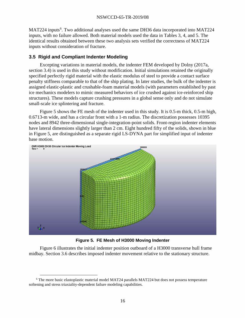
Figure 5 shows the FE mesh of the indenter used in this study. It is 0.5-m thick, 0.5-m high, 0.6713-m wide, and has a circular front with a 1-m radius. The discretization possesses 10395 nodes and 8942 three-dimensional single-integration-point solids. Front-region indenter elements have lateral dimensions slightly larger than 2 cm. Eight hundred fifty of the solids, shown in blue in Figure 5, are distinguished as a separate rigid LS-DYNA part for simplified input of indenter base motion.

Figure 5. FE Mesh of H3000 Moving Indenter

Figure 6 illustrates the initial indenter position outboard of a H3000 transverse hull frame midbay. Section 3.6 describes imposed indenter movement relative to the stationary structure.

6 The more basic elastoplastic material model MAT24 parallels MAT224 but does not possess temperature

softening and stress triaxiality-dependent failure modeling capabilities.


17

Figure 6. Initial Indenter Position Outboard of a H3000 Frame Midbay

The two LS-DYNA material models taking the place of the original rigid material in the green-colored part in Figure 57 account for ice crushing phenomena on a macro scale. These are:

a. Isotropic crushable foam (MAT63): This simple model presumes elastic-perfectly-plastic behavior and requires only yield stress as a function of volumetric strain and a tensile pressure cutoff value.

b. Kinematic/isotropic elastic-plastic material (MAT3): This is a conventional J2 flow theory elastic-plastic material model with choice of kinematic or isotropic hardening and optional ability to account for rate dependency.

Neither of these material models have a “failure” criterion, but one may be introduced via the MAT_ADD_EROSION keyword. MAT63 works only for 3D solid finite elements and cannot be used for thick-shell element modeling of uniform-thickness ice slabs.

LS-DYNA MAT63 has been successfully used in simulation of full-scale ship/iceberg collision (Gagnon & Derradji-Aouet, 2006; Gagnon, 2007), in simulation of laboratory-scale ice crushing tests (Kim, 2014), and in conceptual ice wedge/indenter collision studies (Sazidy, 2015). The material model’s developer originally devised MAT63 parameters on the basis of fitting to full-scale ship/glacial ice impact data (Gagnon, 2007) and later developed less-rigid MAT63 parameter sets on the basis of “hard” and “soft” zone contact pressures measured during ice cone crushing tests including ice splintering and spalling (Gagnon, 2011). A comparison study of the 2007 and 2011 MAT63 parameters (Storheim, 2016, section 7.4) highlights the dramatic rigidity of the 2007 model compared with the 2011 model and an alternative elastic-plastic ice material model with hydrostatic-pressure dependence (Liu, Amdahl, & Løset, 2011b).

This effort considered both the 2007 MAT63 parameter set and another parameter set resembling the 2011 MAT63 set, used in an ice impact test planning effort (Dolny, Daley, Quinton, & Daley, 2017b) and referred to, henceforth, as the “2017b” MAT63 parameter set.

7 The blue-colored part carrying indenter base motions remains rigid.


18

The principal point of commonality between the 2011 and 2017b MAT63 parameters is the limiting yield stress of 50 MPa. The 2007 and 2017b sets have the same low-strain behavior, but the 2007 set rapidly rigidizes above a volumetric strain of 6.5 %, while the 2017b model initially hardens more slowly and then plateaus at the constant 50-MPa stress. Table 7 lists the two sets, which include volumetric-strain-versus-yield-stress curves and a stress cutoff value that does not allow tensile stress increase above 800 MPa.

Table 7. LS-DYNA MAT63 Parameters for Ice Crushing, 2007 and 2017b Parameter Sets

Parameter Value, 2007& and 2017b#

Mass Density 900 kg/m3

Elastic Modulus 9 GPa

Poisson’s Ratio 0.003

Tensile Cutoff Stress 800 MPa

Volumetric Strain, 2007 Yield Stress, 2007 (MPa)

0.0 0.1

0.065 0.1

1.0 4500

Volumetric Strain, 2017b Yield Stress, 2017b (MPa)

0.0 0.1

0.065 0.1

0.075 50

1.0 50 Notes: & 2007 parameters adapted from “Results of Numerical Simulations of Growler Impact Tests,” by R. E. Gagnon, 2007, Cold Regions Science and Technology, 49, 206–214. # 2017b parameters adapted from ONR Ice Capability Assessment and Experimental Planning, Deliverable #3: Experimental Planning for Large Non-Ice Class Grillage Tests [Technical report], by J. Dolny, C. Daley, B. Quinton, and K. Daley, 2017, Houston, TX: American Bureau of Shipping.

Figure 7 dramatizes the substantial differences between the various MAT63 glacial ice volumetric-strain-versus-yield-stress parameter sets. The original 2007 curve, the 2011 curve defined above (labeled M1), and the 2017b curve are compared. It is apparent that the 2017b curve is a combination of the 2007 curve at lower strain and the 2011 (M1) curve at higher strain. The 2011 (M2) curve is a low-pressure zone characteristic (Gagnon, 2011) that is relevant for ice spalling modeling but was not pertinent to this study8.

8 The M1 and M2 labels follow those used by Storheim (2016).


19

Figure 7. Comparison of Volumetric-Strain-versus-Yield-Stress Curves for Various LS-

DYNA MAT63 Ice Models Crushing response of ice has also been successfully modeled (Dolny et al., 2017a; Liu,

Daley, Yu, & Bond, 2012) using LS-DYNA MAT3. Dolny et al. (2017a) performed an optimization study that established MAT3 parameters as a function of ice thickness for ice slabs crushed against a rigid wall. The optimal parameters produced pressure-versus-indentation curves that closely resembled an experimentally based pressure/contact area function widely used to define ice loading on fixed structures and ice-reinforced ships. The parameter most beneficial for data fitting was the presumed MAT3 “yield stress,” which varied moderately for the range of ice slab thicknesses considered by Dolny et al. In this effort, the optimized yield stress for the thickest slab (0.35 m) is used. Table 8 lists the complete MAT3 parameter set. The mass density and elastic modulus are identical to those presumed for MAT63.

Table 8. LS-DYNA MAT3 Parameters for Ice Crushing

Parameter Value

Mass Density 900 kg/m3

Elastic Modulus 9 GPa

Poisson’s Ratio 0.33

Yield Stress 1.2551 MPa

Plastic Hardening (Tangent) Modulus 10 MPa Note: Data adapted from ONR Ice Capability Assessment and Experimental Planning, Deliverable #2: Advanced Modeling and Re-assessment of NSWCCD Hull 3000 [Technical report], by J. Dolny, C. Daley, B. Quinton, and K. Daley, 2017, Houston, TX: American Bureau of Shipping.


20

Strain definitions differ between the MAT63 and MAT3 stress-versus-strain curves (volumetric strain and effective plastic strain, respectively). Nevertheless, the very low initial yield stress and low hardening modulus for MAT3 suggests that ice modeled with the MAT3 parameters will be more compliant than ice modeled with MAT63 and the parameters of Table 7.

3.6 Collision Kinematics Relative rigid indenter/structure (or ice/structure) motions in this study follow displacement

control, a highly prescribed form of two-body collision interaction. All nodes on the periphery of the structure remain fixed. The indenter approaches the structure from a small standoff distance, indents the structure a specified distance, and then slides along the structure with the indentation distance held constant. This denting and scoring action, with the structure responding locally with no rigid body motion allowed, can be highly damaging. It represents the limiting ice/structure interaction case where the mass of the ice body is comparable to or greater than the mass of the ship.

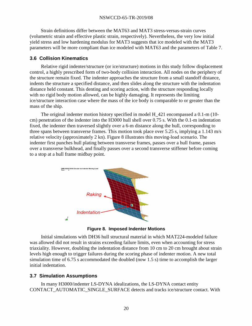
The original indenter motion history specified in model H_421 encompassed a 0.1-m (10-cm) penetration of the indenter into the H3000 hull shell over 0.75 s. With the 0.1-m indentation fixed, the indenter then traversed slightly over a 6-m distance along the hull, corresponding to three spans between transverse frames. This motion took place over 5.25 s, implying a 1.143 m/s relative velocity (approximately 2 kn). Figure 8 illustrates this moving-load scenario. The indenter first punches hull plating between transverse frames, passes over a hull frame, passes over a transverse bulkhead, and finally passes over a second transverse stiffener before coming to a stop at a hull frame midbay point.

Figure 8. Imposed Indenter Motions

Initial simulations with DH36 hull structural material in which MAT224-modeled failure was allowed did not result in strains exceeding failure limits, even when accounting for stress triaxiality. However, doubling the indentation distance from 10 cm to 20 cm brought about strain levels high enough to trigger failures during the scoring phase of indenter motion. A new total simulation time of 6.75 s accommodated the doubled (now 1.5 s) time to accomplish the larger initial indentation.

3.7 Simulation Assumptions In many H3000/indenter LS-DYNA idealizations, the LS-DYNA contact entity

CONTACT_AUTOMATIC_SINGLE_SURFACE detects and tracks ice/structure contact. With


21

this contact algorithm, all free faces of all elements in the model are candidates for contact and sliding. However, since all structural elements are shells, it makes little sense to include all interior structural elements (decks, floors, stiffeners) as candidate contact surfaces. Therefore, the structural contact surfaces are restricted only to the parts comprising the water-exposed side shell. In cases where hull side shell structural element failure took place, “eroding” contact algorithms CONTACT_ERODING_SINGLE_SURFACE and CONTACT_ERODING_SURFACE_TO_SURFACE were tested, but the lengthened run times did not justify the inconsequential differences in results.9 Runs with compliant instead of rigid indenters used CONTACT_AUTOMATIC_SURFACE_TO_SURFACE, again with restriction to selected parts, but contact results did not significantly change with respect to the single-surface algorithm.

LS-DYNA allows modeling of nonzero contact surface friction with classical Coulomb friction assumptions, and it allows optional assignment of distinct static and dynamic friction properties. Most simulations in this effort presumed zero ice/structure interface friction, but a few concluding simulations considered nonzero static and dynamic friction following available test data for steel-on-ice contact. Details of friction modeling assumptions follow in specific analysis discussions.

The LS-DYNA contact entity CONTACT_FORCE_TRANSDUCER_PENALTY recovers forces on all structural contact surface faces, the sum of which obtains the total load exerted on the H3000 side shell. Time histories of this force are fundamental bases of comparison between the many simulations.

The structure/ice slab interaction simulations reported by Lesar (2019) included buoyancy loading on the ice slabs, exploiting the DEFINE_FUNCTION modeling feature of LS-DYNA. In the present simulations, indenter motion is totally prescribed, and buoyancy effects are irrelevant; thus, DEFINE_FUNCTION is unnecessary.

LS-DYNA’s default viscous hourglassing10 control algorithm with the default coefficient of 0.10, successful in prior ice slab impact analyses (Lesar, 2019) also proved effective in the present rigid indenter simulations. However, this assumption failed to produce reasonable indenter deformations and low indenter hourglass energy when MAT3 or MAT63 replaced the rigid indenter material. The stiffness hourglass control algorithm better minimized hourglass energy in simulations including compliant indenters.

For modeler information, LS-DYNA computes the maximum time step implied by all structural elements and contact surfaces for explicit time integration stability. The maximum time step implied by contact surfaces was slightly lower than the step implied by structural (or indenter) elements (2.225e-6 s versus 2.4075e-6 s, respectively). The LS-DYNA-computed time step prevailed in early analyses, but a CONTROL_TIMESTEP-enforced time step of 2.2e-6 s was specified for later runs.

9 Eroding contacts would be far more necessary if indenter element deletion took place. 10 “Hourglassing” is non-physical element-level zero-energy mode response that occurs in underintegrated

elements used in explicit time domain analysis codes. While never totally suppressed unless more computationally expensive fully or selectively integrated elements are used, hourglassing may often be reduced to negligible levels by imposing carefully targeted artificial damping, stiffness, or both. In some circumstances not always readily foreseeable, fully or selectively integrated element usage is necessary.


22

Text-format (ASCII) data for time-history plotting (principally contact surface forces and energy metrics) is saved at 0.006-s intervals (1000 samples in 6.0 s), and binary whole-model data is saved at 0.12-s intervals (50 samples in 6.0 s). Time history and full-model-state sampling intervals increased to 0.00675 s and 0.135 s for simulations with a 6.75-s time span. The resultant contact force (RCFORC) file contained required contact surface force and moment time histories. The binary datasets provided inelastic strain contours and animations of structure and ice deformations including development of structural fractures.

3.8 Simulation Hardware and Code Versions U.S. Department of Defense High Performance Computing Center resources supported all

simulations reported here, specifically, the LS-DYNA code installed on the Air Force Research Laboratory (AFRL) computing system. The initial code version used was massively parallel LS-DYNA version mpp-s-Dev, revision 103383, run in single precision. Although this version (“v8”) was system “default”, it produced physically implausible results when MAT224 element failures occurred. Subsequently, newer, nondefault LS-DYNA versions 10 (mpp-s R10.1.0 rev 123264) and 11 (mpp-s R11.0.0 rev 129956) were invoked.

Computing hardware was the AFRL SGI IceX 5.62 PFLOPS 3216-core platform thunder. Depending on H3000 material and ice/structure contact modeling options chosen, LS-DYNA jobs completed within 1.5 h to 4 h of wall-clock time under “standard” queue priority with initially 24 processors in earlier runs and 36 processors in later runs. Usage of MAT224 increased run times about 50 % above times required with MAT24, and eroding contact surfaces increased run times about 25 % above times required for noneroding contact.


23

4. Results and Discussion

This section documents the several dozen LS-DYNA ice/structure collision simulations carried out. The analyses fall into four major groups.

• Rigid Indenter Simulations without Structural Fracture Occurrence:The first group encompassed preliminary analyses directly extended from the moving-ice-load simulations of Dolny et al. (2017a), substituting HY80 steel with lower-strength DH36. Although LS-DYNA material model MAT224 functioned as expected for both rate-dependent and rate-independent properties, the indenter penetration was not high enough to trigger hull shell rupture and tearing.

• Rigid Indenter Simulations with Reduced Structural Failure Strains. The second group of simulations accomplished hull steel failure by presuming artificially lower DH36 failure strains. These analyses allowed debugging of MAT224 failure-strain input and revealed sensitivity of MAT224 computations to LS-DYNA code version and modeling choices. Usage of contact surface options accounting for contact surface adjustments due to element failure (“erosion”) did not appreciably change structural damage results. However, structural failure degree showed large sensitivity of strain evolution to load-path dependence assumptions chosen for MAT224.

• Rigid and Glacial Ice Indenter Simulations with Realistic Structural Failure Strains and Doubled Initial Penetration. Using the more damaging load-path dependence option, the third group of analyses accomplished hull shell rupture and tearing by doubling the indenter’s penetration distance. Simulations in this group used the original rigid indenter material and a material model often applied to the modeling of glacial ice. These runs revealed strong dependency of dynamic response solution quality on the chosen hourglassing control method and contact surface algorithm choice.

• Compliant Ice Indenter Simulations with Doubled Initial Penetration. A fourth analysis series considered LS-DYNA models representing ice with various crushing compliance levels. These analyses showed drastic dependence of predicted structural damage levels on indenter rigidity, with relatively little damage inflicted by the most compliant ice body. Simulations including indenter/structure contact surface friction for all ice approximations showed very little effect.

The above four analysis series are discussed in turn in subsections 4.1 to 4.4.

4.1 Rigid Indenter Simulations without Structural Fracture Occurrence All simulations in this group presumed the same indenter motions over a 6-s time span, as

assumed by Dolny et al. (2017a): 10-cm indentation followed by ~ 6-m scoring movement. All cases used a rigid indenter and viscous hourglass control with the default coefficient, and they all applied the automatic single-surface contact algorithm with zero interface friction. Table 9 lists particulars of the eight LS-DYNA runs accomplished, all using 24 thunder central processing


24

units (CPUs). The parameter failopt indicates the chosen MAT224 load-path dependence option. Note the inclusion of baseline runs using MAT24, a basic elastoplastic material model that does not possess the advanced failure modeling capabilities of MAT224, as discussed in section 3.4.

Table 9. Particulars of LS-DYNA Group 1 Analyses

LS-DYNA Run ID

Hull Material Model

Failure Option

Rate dependence

LS-DYNA Version

Wall-clock time

Time step (s)

10763 MAT24 none no 8 1 h 39 min 2.41e-6

35402 MAT24 none yes 8 1 h 38 min 2.41e-6

45158 MAT224 none no 8 2 h 58 min 2.41e-6

24631 MAT224 none yes 8 2 h 49 min 2.41e-6

48726 MAT224 failopt 0 no 8 2 h 57 min 2.41e-6

16262 MAT224 failopt 0 yes 8 2 h 53 min 2.41e-6



Note: All runs assumed rigid indenter, automatic single surface contact, no interface friction, default viscous hourglass control.

Of available detailed analysis results, time histories of the resultant contact force acting between the indenter and the hull structure are the most important. These are provided in numerous comparisons between simulations. Peak contact forces, number of deleted elements in cases with allowed failure, and peak inelastic strains over the entire structure and in the indenter-loaded side shell are compared in tables. Failure pattern displays and contour plots of inelastic strain fields appear where needed and appropriate.

4.1.1 Comparison of MAT24 with MAT224 Table 10 lists the maximum (max) contact force resultants and peak inelastic strains for the

first four runs listed in Table 9.


25

Table 10. Peak Contact Forces and Inelastic Strains for LS-DYNA Group 1 Analyses, MAT24/MAT224 Correlation

LS-DYNA Run ID

Hull Material Model

Rate Dependence

Maximum Contact Force (MN)

Time of Max

Force (s)

Peak Plastic Strain in Hull Shell

Peak Plastic Strain in

Entire Structure

10763 MAT24 no 1.664 3.35 0.1865 0.3719

35402 MAT24 yes 1.862 3.38 0.1799 0.3640

45158 MAT224 no 1.664 3.37 0.1855 0.3768

24631 MAT224 yes 1.843 3.34 0.1759 0.3680

Simulation results using MAT24 and MAT224 (with no failure allowed) for both rate-

dependent and rate-independent DH36 stress-strain curves confirm the near-equivalence of the two elastic-plastic models for no-failure conditions. This is evident from the close agreement between runs 10763 and 45158 and between runs 35402 and 24631 in Table 10. In parallel with analyses reported by Dolny et al. (2017a), both MAT24 and MAT224 demonstrated a modest strengthening effect when material rate dependence is included in material property definitions. This is evident from the differences between runs 10763 and 35402 and between runs 45158 and 24631 in Table 10. Account of rate dependence on strength brings about higher contact force with less permanent set damage.

As MAT24 and MAT224 results are only modestly different, rate-dependence impact on resultant contact force is displayed only for MAT224. Figure 9 contains a resultant force-to-time- history comparison between runs 45158 and 24631.

Figure 9. Resultant Contact Force Histories for Rate-Independent and Rate-Dependent

DH36 Steel Properties


26

Figure 10 compares final effective-plastic-strain contours for cases 45158 and 24631.

(a) Rate-Independent Properties

(b) Rate-Dependent Properties

Figure 10. Final Effective-Plastic-Strain Contours for Rate-Independent and Rate-Dependent DH36 Steel Properties

4.1.2 MAT224 Parameter Definition Checks This section discusses MAT224 simulation results for cases where structural failure is

allowed in LS-DYNA run case input. Table 11 lists the maximum contact forces and peak inelastic strains for the last four runs of Table 9.


27

Table 11. Peak Contact Forces and Inelastic Strains for LS-DYNA Group 1 Analyses, MAT224 Parameter Definition Checks

LS-DYNA Run ID

Failure Option

Rate Dependence

LS-DYNA

Version


Time of Max

Force (s)

Peak Plastic Strain in Hull Shell

Peak Plastic

Strain in Entire

Structure

48726 failopt 0 no 8 1.664 3.37 0.1855 0.3768

16262 failopt 0 yes 8 1.843 3.34 0.1759 0.3680

49180 failopt 1 no 8 1.657 3.37 0.1873 1.7510

50813 failopt 0 no 10 1.666 3.38 0.1852 0.3771

Runs 48726 and 16262 agreed exactly with runs 45158 and 24631, respectively, showing

that the 10-cm indentation magnitude is too low for failure to occur. This result prompted a check on MAT224 “failure options” chosen through the failopt parameter.

All analyses thus far assumed the load-path dependent method of computing strain accumulation to failure, failopt = 0. Run 49180 is a redo of run 48726, with failopt toggled to the load-path independent method. Data in Table 11 show that contact force and hull shell plastic-strain differences were minor, but nonsensical, entire-model plastic-strain maxima occurred when failopt was set to 1 (see the grey cell in Table 11). This unexpected result led to run 50813, where the thunder run submittal pointed to the newest available nondefault LS-DYNA code version 10. The intention was to retain failopt = 1, but failopt = 0 was mistakenly retained, repeating run 48726 rather than 49180. No suspicious effective-plastic-strain results resulted between LS-DYNA versions 8 and 10 with the load-path dependent effective-strain-incrementation method.

In summary, analysis group 1 proved that LS-DYNA materials MAT24 and MAT224 behave nearly identically for no-failure conditions. Material strength strain-rate dependence is important even at the relatively modest dynamic rates prevailing in these indenter/structure analyses. Sensitivity of computations to load-path dependence method exists, though an LS-DYNA version integrity issue clouds this evaluation.

Continuing MAT224 failure parameter exploration and confirmation of LS-DYNA version problems appeared to be unfruitful in simulations where material strength assumptions relative to loading were not allowing failure. For this reason, rather than changing loading magnitude and time history, stress-triaxiality-dependent failure strains were artificially lowered by a factor of two in the subsequent analysis groups.

4.2 Rigid Indenter Simulations with Reduced Structural Failure Strains All simulations in this group presumed the same indenter motions over a 6-s time span as

assumed by Dolny et al. (2017a): 10-cm indentation followed by ~ 6-m scoring movement. All cases used a rigid indenter and viscous hourglass control with the default coefficient, and they all included material rate dependence and zero interface friction. Table 12 lists particulars of the


28

seven LS-DYNA runs accomplished, all but the last using 24 thunder CPUs. Run time beneficially decreased with 36 CPUs. In the latter runs of this analysis group, a newer non-system-default LS-DYNA code release (version 10) overcomes a suspected flaw in version 8.


LS-DYNA Run ID

Failure option

Contact Type LS-DYNA

Version

CPUs Wall-Clock Time

Time Step (s)

29686 failopt 0 Single surface 8 24 2 h 54 min 2.41e-6




46915 failopt 1 Eroding single surface

10 24 3 h 21 min 2.00e-6*

45236 failopt 1 Eroding surface to surface

10 24 3 h 12 min 2.00e-6*

36896 failopt 1 Eroding single surface

10 36 2 h 17 min 2.00e-6*

Notes: All runs assumed rigid indenter, MAT224 with rate dependence, no interface friction, default viscous hourglass control, failure strains in stress-triaxiality curve lowered by factor of two from group 1. * Maximum 2.2e-6 s time step specified; LS-DYNA takes a smaller time step than minima indicated for all elements and contact surfaces. Curiously, with eroding contact surfaces specified, LS-DYNA takes a time step lower than

the minimum-element and contact-surface time steps declared in the main-text-format output file d3hsp. The reason is unclear.

4.2.1 LS-DYNA Code Version Check and Failopt Parameter Influence The first four analyses listed in Table 12 systematically examine the LS-DYNA version

issue occurring with the MAT224 failure option enabled, and provide “clean” information on the impact of MAT224 failure option choice. Table 13 contains contact force, hull shell element failure, and structural model effective-plastic-strain data for these four cases.


29

Table 13. Peak Contact Forces and Inelastic Strains for LS-DYNA Group 2 Analyses, MAT224 Failure Criteria Checks

LS-DYNA Run ID

Failure Option

LS-DYNA

Version


Time of Max Force

(s)

Number of Failed

Structural Elements

Time of First

Element Failure

(s)

Peak Plastic

Strain in Hull Shell


Entire Structure

29686 failopt 0 8 1.777 3.33 61 3.36 0.8757 0.8757

27805 failopt 1 8 1.320 3.32 132 0.85 0.8757 0.8757

49372 failopt 0 10 1.776 3.33 61 3.36 0.1669 0.3639

21496 failopt 1 10 1.347 3.33 130 0.85 0.1365 0.3516

LS-DYNA version 8 runs 29686 and 27805 with failopt = 0 and failopt = 1 provided

invalid effective-plastic-strain results (see grey cells in Table 13). Nevertheless, computed hull shell displacement and Von Mises stress results (not reproduced here) seemed valid. This anomaly could be a results-database-integrity problem peculiar to MAT224 in LS-DYNA version 8 when failure occurs. In runs 49372 and 21496, LS-DYNA version 10 produced no obvious invalidity in reported effective plastic strains.

LS-DYNA results differ in major ways between MAT224 failopt = 0 and failopt = 1. The load-path independent method of incrementing effective plastic strain, failopt = 1, provided significantly greater structural tearing damage, reducing the peak force sustained during indenter/hull structure interaction. Figure 11 compares contact force time histories for runs 49372 and 21496, and it also includes a no-failure baseline curve from run 24631. Once structural rupture occurs and tearing begins, the load-carrying capability of the hull shell drops significantly.

Figure 11. Resultant Contact Force Histories for Two MAT224 Failure Options


30

Figure 12 compares the final tearing damage patterns and permanent set strains for cases 49372 and 21496. In the fomer case, tearing does not begin until after the indenter traverses the deep transverse hull frame. In the latter case, tearing commences immediately after initial indentation.

(a) Load-Path Dependence

(b) Load-Path Independence

Figure 12. Final Effective-Plastic-Strain Contours and Tearing Damages for Two MAT224 Failure Options

The strong dependence of structural damage extent on the MAT224 failure criteria is concerning and deserves both computational and experimental evaluation. It is natural to include failure criteria choice in pretest and posttest simulations of experiments that attain plating rupture. A relatively recent set of unstiffened and stiffened plate penetration experiments (Alsos


31

& Amdahl, 2009) and parallel analyses (Alsos, Amdahl, & Hoppersatd, 2009) provide excellent experimental data and comparative simulation data for this purpose and will be the subject of a future report.

4.2.2 Eroding Contact Surface Evaluation In LS-DYNA, “eroding” contact surfaces allow faces on elements deleted due to material

failure to be eliminated from consideration for contact with faces on nonfailed elements. This is important in complex dynamic failure simulations with fragmentation and debris formation where postfailure interaction of broken pieces is important. In the present case, indenter fracture (and rubble formation) is not allowed, and structural tearing is follows a relatively linear path. The chief reason for employing an eroding contact is to obtain postprocessing displays of contact surface pressures and forces that account for structural element deletion.

Table 14 contains contact force, hull shell element failure, and structural model effective-plastic-strain data for the three eroding contact simulation cases attempted. Table 14 also contains data for run 21496, which used noneroding contact and acted as a comparison baseline.

Table 14. Peak Contact Forces and Inelastic Strains for LS-DYNA Group 2 Analyses, Eroding Contact Evaluations

LS-DYNA Run ID

Contact Type


Time of Max

Force (s)

Number of Failed

Structural Eements

Time of First

Element Failure

(s)

Peak Plastic



Entire Structure

21496 Single surface

1.347 3.33 130 0.85 0.1365 0.3516

46915 Eroding single

surface

1.354 3.27 134 0.85 0.1113 0.3437

45236 Eroding surface

to surface

1.527 3.29 69 3.30 0.1402 0.3132

36896 Eroding single

surface

1.348 3.33 129 0.85 0.1145 0.3482

The first point of comparison is between runs 21496 and 46915, the only difference being

an eroding single surface contact in 46915 versus a noneroding contact in 21496 (failopt = 1 applies in both). Results are not identical but close, with four more elements reaching failure with the eroding contact. Figure 13 compares the nearly identical resultant contact force time histories for runs 21496 and 46915.


32

Figure 13. Resultant Contact Force Histories for Noneroding and Eroding Contacts

Figure 14 shows very little difference in tearing damage pattern and permanent set strains between cases 21496 and 46915. The chief difference between the two analyses is the eroding contact run requiring 25 % greater run time.

(a) Noneroding Contact

Figure 14. Final Effective-Plastic-Strain Contours and Tearing Damages for Noneroding and Eroding Contacts


33

(b) Eroding Contact

Figure 14. Final Effective-Plastic-Strain Contours and Tearing Damages for Noneroding and Eroding Contacts (cont’d)

In run 45236, the surface-to-surface contact option more precisely circumscribes candidate contact surfaces than the single-surface specification of run 46915. Table 14 data indicates significant differences in contact forces and extent of failure between eroding single-surface contact (run 46915) and eroding surface-to-surface contact (run 45236). Figure 15 illustrates contact force differences, and Figure 16 contrasts the different tearing damage patterns. For unknown reasons, usage of surface-to-surface contact delayed tearing damage onset until the moving indenter traversed the stiff bulkhead.

Figure 15. Resultant Contact Force Histories for Eroding Contact Options


34

(a) Single Surface Contact

(b) Surface-to-Surface Contact

Figure 16. Final Effective-Plastic-Strain Contours and Tearing Damages for Eroding Contact Options

Run 36896 is nearly identical to run 46915 except that 36 CPUs are requested rather than 24, and output data writing to LS-DYNA’s binary file group for contact surface data is more complete. Essentially the same results occur, but deployment of additional CPUs more than recovers the run-time penalty.

In summary, analysis group 2 unambiguously identified an inelastic strain output deficiency with a particular LS-DYNA code version, which should be avoided when using MAT224. Structural damage extent computations showed strong dependence on the MAT224


35

load-path dependence approach. LS-DYNA contact entities accounting for contact surface erosion due to element deletion produced damage results of unclear integrity.

Absent experimental data for simulation correlation, it is not clear whether eroding contact usage for this problem area is necessary or worthwhile. Further analyses in this effort did not consider this modeling complication, though it is worthy of revisit in future analysis/experiment correlations.

4.3 Rigid and Glacial Ice Indenter Simulations with Realistic Structural Failure Strains and Doubled Initial Penetration

To induce material damage without arbitrary change in failure strains, all further analyses in this effort presumed hull shell indentations of 20 cm rather than 10 cm. A doubling of the time span of indenter motion normal to the hull shell from 0.75 s to 1.5 s maintained the initial loading rate. To maintain the same scoring distance, the total simulation time span increased from 6.0 s to 6.75 s. All cases used LS-DYNA version 10 and included material rate dependence, failopt = 1, and zero interface friction.

A new rigid indenter baseline analysis was carried out for the doubled penetration distance; additionally, MAT63 with Gagnon (2007) parameters, the ice crushing material model calibrated for glacial ice, was considered. Reasonable results with the glacial ice indenter required variations in contact surface options and hourglass control methods beyond those that were successful for the rigid indenter. Table 15 lists particulars of the seven LS-DYNA runs accomplished, all using 36 thunder CPUs.


36


LS-DYNA Run ID

Indenter Material

Contact Type

Hourglass Control

LS-DYNA

Version

Wall-Clock Time

(h, min)

Time Duration

(s)

Time Step (s)

17312 Rigid Single surface

Viscous 10 2 h 18 min 6.0 2.20e-6


Viscous 10 2 h 36 min 6.75 2.20e-6

52169 MAT63 (Gagnon,

2007)&

Single surface

Viscous 11 1 h 18 min* 2.5* Cut to 1.71e-6


2007)&

Single surface

Stiffness 11 2 h 0 min* 2.5* 2.20e-6


2007)&

Single surface, soft = 1

Stiffness 11 2h 58 min 6.75 2.20e-6


2007)&

Surface to surface

Viscous 11 4 h 16 min 6.75 Cut to 1.08e-6


2007)&

Surface to surface

Stiffness 11 3 h 5 min 6.75 2.20e-6

Notes: All runs assumed MAT224 with rate dependence, failopt = 1, no interface friction, and 36 CPUs. & These runs used MAT63 ice model reported in “Results of Numerical Simulations of Growler Impact Tests,” by R. E. Gagnon, 2007, Cold Regions Science and Technology, 49, 206–214. * These runs limited to 2.5-s dynamic event duration for debugging purposes.

The first analysis in Table 15 is of little interest except as a comparison with earlier runs; analysis 6313 serves as a new rigid indenter comparison baseline for the glacial ice variation. It should be noted that failopt = 1 is chosen in these and all subsequent simulations. At present, this is an arbitrary choice not yet supported by experimental data for ice-loaded ductile steel structures suffering rupture and tearing damage.

4.3.1 Initial Glacial Ice Indenter Simulations Four cases listed in Table 16 concern initial attempts to obtain an acceptably stable solution

for the MAT63 indenter with Gagnon (2007) parameters. Table 16 contains contact-force and hull-shell-element-failure results for rigid indenter baseline run 6313 plus three MAT63 indenter simulation attempts. Initial MAT63 runs (52169 and 56915) using automatic, single-surface contact and both viscous and stiffness hourglass control methods suffered crippling hourglassing response prior to half of the planned simulation time span. In these cases, the compliant ice indenter dominated the total model hourglass energy. However, choosing the soft = 1 algorithm for computing contact penalty stiffnesses (basing on nodal masses and global time step size


37

rather than bulk moduli of the contacting materials) had a beneficial effect, producing a plausibly valid solution for the case with MAT63 ice. The LS-DYNA developer recommends the soft = 1 penalty stiffness option in situations where the bulk moduli of the two contacting media differ greatly, particularly “soft foams” and metals (LSTC, 2017, Vol. I, page 11-71). Table 16. Peak Contact Forces and Failure Results for LS-DYNA Group 3 Analyses, Initial

MAT63 Indenter Modeling Attempts

LS-DYNA Run ID

Indenter Material&

Contact Type

Hourglass Control


Time of Max

Force (s)

Number of Failed

Structural Elements

Time of First

Element failure

(s)


Viscous 2.105 1.49 133 2.256


2007)&

Single surface

Viscous Poor quality solution before 2.5 s


2007)&

Single surface

Stiffness Poor quality solution before 2.5 s


2007)&


Stiffness 2.573 3.94 80 2.248

Note: & These runs used the MAT63 ice model reported in “Results of Numerical Simulations of Growler Impact Tests,” by R. E. Gagnon, 2007, Cold Regions Science and Technology, 49, 206–214.

Figure 17 compares the resultant contact force time histories for rigid and glacial ice indenters from runs 6313 and 56707. The nonrigid indenter initially exerts less force on the hull. However, since it does not weaken the hull by tearing after passing the first transverse stiffener, it exerts greater peak force than the rigid indenter when loading the transverse bulkhead. Tearing initiates after the bulkhead, and the two indenters exert similar forces thereafter.


38

Figure 17. Resultant Contact Force Histories for Rigid and MAT63 Indenters

Figure 18 compares final tearing damage patterns and permanent set strains between cases 6313 and 56707. The less-rigid indenter leaves the first- and second-traversed frame bays intact, but both indenters tear the third- and fourth-traversed frame bays similarly. The wider opening gouged into the hull plating by the MAT63 indenter stands in contrast with the narrow slot inflicted by the rigid indenter.

(a) Rigid Indenter

Figure 18. Final Effective-Plastic-Strain Contours and Tearing Damages for Rigid and MAT63 Indenters


39

(b) MAT63 Indenter

Figure 18. Final Effective-Plastic-Strain Contours and Tearing Damages for Rigid and MAT63 Indenters (cont’d)

4.3.2 Additional Glacial Ice Indenter Simulations Although simulation 56707 provided a plausible rupture and tearing solution for a MAT63

indenter with original Gagnon ice parameters, the sensitivity with respect to hourglass control and contact surface penalty stiffness prompted a check as to whether an alternative LS-DYNA contact surface algorithm resulted in cleaner model behavior. Two additional runs, using viscous and stiffness-based hourglass control methods, considered replacement of the CONTACT_AUTOMATIC_SINGLE_SURFACE entity with CONTACT_AUTOMATIC_SURFACE_TO_SURFACE. Table 17 contains resultant contact force and hull structure failure results for the two additional MAT63 simulations, with the most successful initial MAT63 simulation included as a baseline. The two runs (56707 and 19528) utilizing stiffness hourglass control but different contact surface definition methods produced very similar results. As in the initial analysis set summarized in Table 16, viscous hourglass control (run 44129) underperformed, with high hourglass-to-kinetic-energy ratio compared to when stiffness control is used.


40

Table 17. Peak Contact Forces and Failure Results for LS-DYNA Group 3 Analyses, Additional MAT63 Indenter Modeling Attempts

LS-DYNA run ID

IndenterMaterial

Contact Type

Hourglass Control


Time of Max force

(s)

Number of Failed

Structural Elements

Time of First

Element Failure

(s)


2007)


Stiffness 2.573 3.94 80 2.248


2007)

Surface to surface

Viscous 2.533 3.93 29 2.277


2007)

Surface to surface

Stiffness 2.538 3.94 79 2.285

Note: All runs used MAT63 ice model reported in “Results of Numerical Simulations of Growler Impact Tests,” by R. E. Gagnon, 2007, Cold Regions Science and Technology, 49, 206–214.

The performance of the single-surface and surface-to-surface contact surface specification algorithms is of interest. Figure 19 compares the resultant contact force time histories for nonrigid indenters from runs 56707 and 19528. Except for the latter stages of the event, the two analyses for differing LS-DYNA contact definitions agree closely. This figure also includes the contact-force curve for lower-quality analysis 44129. The use of surface-to-surface contact provided lower final inelastic strain levels than when single-surface contact is used; however, the hourglassing energy in run 19528 is lower than in run 56707, indicating a point in favor of the surface-to-surface contact option.

Figure 19. Resultant Contact Force Histories with MAT63 Indenters for Alternative

Contact Surface and Hourglass Control Assumptions


41

Figure 20 compares final tearing damages and permanent set strains produced in runs 44129 and 19528. The lesser tearing damage produced in the viscous hourglass control run is obvious.

(a) Viscous Hourglass Control

(b) Stiffness Hourglass Control

Figure 20. Final Effective-Plastic-Strain Contours and Tearing Damages with MAT63 Indenters for Alternative Contact Surface and Hourglass Control Assumptions

In summary, analysis group 3 revealed a strong sensitivity of indenter/structure interaction solution quality to LS-DYNA hourglass control method when a nonrigid indenter is modeled with a glacial-ice-calibrated LS-DYNA crushable foam material model. In this case, the nondefault, stiffness-based method provided greatly superior hourglassing control. Hourglassing suppression also improved with usage of the surface-to-surface contact detection method.


42

Computed structural rupture and tearing damage results indicated, reasonably, less rupture and tearing damage with a compliant indenter versus a rigid indenter.

4.4 Compliant Ice Indenter Simulations with Doubled Initial Penetration A final LS-DYNA simulation group considered less-rigid variations of the MAT63

crushable foam material model calibrated for ice, and the MAT3-based elastic-plastic ice crushing approximation. All analyses in this effort presumed hull shell indentation of 20 cm in 1.5 s and sliding loading over a 5.25-s time span. In all cases, newly available LS-DYNA version 11 is used, material rate dependence is included, MAT224 failopt = 1, and the automatic surface-to-surface contact surface specification is used. Analyses also reconsidered viscous hourglass control and elimination of indenter hourglassing by usage of selective/reduced integration 3D solid elements.

New rigid-indenter baseline analyses were carried out for frictionless contact and contact with static and dynamic friction calibrated to represent in-field experimental data for ice sliding on corroded steel. The final analyses for compliant indenters introduced contact friction.

Table 18 lists particulars of the seven LS-DYNA runs accomplished, all using 36 thunder CPUs.


43


LS-DYNA Run ID

Indenter Material

Hourglass Control

Contact Surface Friction

Wall-Clock Time Time Step (s)

31751 Rigid Stiffness No 2 h, 34 min 2.20e-6

42278 MAT63 (Dolny, 2017b)#

Viscous No Aborted 2.20e-6, cut to 1.54e-6

45552 MAT63 (Dolny, 2017b)#

Stiffness No 3 h, 5 min 2.20e-6

52800 MAT63 (Dolny, 2017b)#

Stiffness* No Run aborted 2.20e-6, goes negative

895 MAT3 (Dolny, 2017a)@

Stiffness No 3 h, 45 min 1.80e-6, cut to 9.26e-7**

12251 Rigid Stiffness Yes 4 h,16 min 2.20e-6

7816 MAT63 (Dolny, 2017b)#

Stiffness Yes 3 h, 5 min 2.20e-6

8737 MAT3 (Dolny, 2017a)@

Stiffness Yes 3 h, 37 min 1.80e-6, cut to 1.27e-6

Notes: All runs assumed MAT224 with rate dependence, failopt = 1, surface-to-surface contact, LS-DYNA version 11, 36 CPUs. # These runs used the MAT63 ice model reported in ONR Ice Capability Assessment and Experimental Planning, Deliverable #3: Experimental Planning for Large Non-Ice Class Grillage Tests [Technical report], by J. Dolny, C. Daley, B. Quinton, and K. Daley, 2017, Houston, TX: American Bureau of Shipping. * Selective/reduced integration 3D solid elements in ice body @ These runs used the MAT3 ice model reported in ONR Ice Capability Assessment and Experimental Planning, Deliverable #2: Advanced Modeling and Re-assessment of NSWCCD Hull 3000 [Technical report], by J. Dolny, C. Daley, B. Quinton, and K. Daley, 2017, Houston, TX: American Bureau of Shipping.

The parameters of the new rigid-indenter baseline run (31751) follow those found to be

most optimal for simulation of structural loading by glacial ice (Gagnon, 2007). These depart from the prior rigid-indenter baseline analysis in two respects: (1) the contact surface option, and (2) the hourglass control option. However, the two analyses provided virtually identical contact force time histories. The new baseline run produced slightly greater tearing damage, and final inelastic strains were lower than in the prior baseline. These differences point to the need to consider hourglass control and contact surface options in future methods-validation exercises, but they do not detract from run 31751 as a suitable baseline for this simulation group.

4.4.1 Compliant Ice Indenter Simulations without Contact Friction Four group 4 simulations listed in Table 18 considered two indenter material property

assumptions reflecting ice that is less rigid than the MAT63 glacial ice approximation. These are the Dolny et al. (2017a, 2017b) models, implemented in LS-DYNA materials MAT3 and MAT63, respectively. LS-DYNA input parameters for these models have been shown in Table 7 and Table 8. Although stiffness-based hourglass control proved superior for the MAT63 glacial


44

ice (Gagnon, 2007) approximation, viscous hourglass control and usage of selective/reduced integration 3D solid elements that lack zero-energy modes were considered.

Table 19 contains contact force, hull shell element failure, and structural model effective-plastic-strain data for the four compliant-indenter cases attempted; it also contains data for run 31751, which used a rigid indenter, to act as a comparison baseline.

Table 19. Peak Contact Forces and Inelastic Strains for LS-DYNA Group 4 Analyses, Frictionless Contact

LS-DYNA Run ID

Indenter Material

Hour-glass

Control


Time of Max

Force (s)

Number of Failed

Structural Elements

Time of First

Element Failure

(s)

Peak Plastic


Peak Plastic

Strain in Entire

Structure

31751 Rigid Stiffness 2.106 1.49 139 2.253 0.2506 0.5037

42278 MAT63 (Dolny, 2017b)#

Viscous Run aborted with segmentation fault at 3.868 s

45552 MAT63 (Dolny, 2017b)#

Stiffness 2.514 3.96 3 2.244 0.2468 0.4500

52800 MAT63 (Dolny, 2017b)#

Stiffness S/R Integration in indenter solid elements. Run aborted with negative time step at 3.869 s

895 MAT3 (Dolny,

2017a)@

Stiffness 2.178 4.04 0 Not applicable

0.1431 0.2607

Notes: # Runs used the MAT63 ice model reported in ONR Ice Capability Assessment and Experimental Planning, Deliverable #3: Experimental Planning for Large Non-Ice Class Grillage Tests [Technical report], by J. Dolny, C. Daley, B. Quinton, and K. Daley, 2017, Houston, TX: American Bureau of Shipping. @ Runs used the MAT3 ice model reported in ONR Ice Capability Assessment and Experimental Planning, Deliverable #2: Advanced Modeling and Re-assessment of NSWCCD Hull 3000 [Technical report], by J. Dolny, C. Daley, B. Quinton, and K. Daley, 2017, Houston, TX: American Bureau of Shipping.

Again, viscous hourglass control was relatively ineffective (in run 42278) for suppressing zero-energy modes in the indenter during raking motion. Surprisingly, usage of selective/reduced integration elements in the compliant indenter failed to provide a stable solution during indenter traversal over the stiff bulkhead.

Figure 21 compares the resultant contact force time histories for nonrigid indenters from runs 45552 and 895 with rigid indenter results from run 31751, as baseline. Contrasting phenomena occur during the initial indentation phase (up to 1.5 s) and the sliding phase (after 1.5 s). Peak load develops after initial indentation increases as indenter rigidity increases. If little


45

or no structural tearing damage occurs, the ordering of load with indenter rigidity continues during the sliding phase. However, sustained load drops sharply if structural tearing occurs11.

Figure 21. Resultant Contact Force Histories for Rigid, MAT63, and MAT3 Compliant

Indenters, Zero Interface Friction Figure 22 compares final tearing damages and permanent set strains produced in runs

45552 and 895 with rigid indenter results from run 31751, as baseline. The compliant indenter from case 45552 produces almost no tearing damage compared to the rigid indenter case 31751, though permanent set strains are only slightly lower in the compliant-indenter case. It is possible that the structural deformations produced by the compliant indenter are close to a threshold for tearing damage. The most compliant indenter of all considered, in case 895, produces no tearing damage at all and inelastic strains that are about half of those resulting in rigid and intermediate-rigidity indenter analyses.

11 Of course, allowance of indenter material damage will change this relatively simple load/indenter rigidity

relationship.


46

(a) Rigid Indenter

(b) MAT63 Indenter

Figure 22. Final Effective-Plastic-Strain Contours and Tearing Damages for Rigid, MAT63, and MAT3 Compliant Indenters, Zero Interface Friction


47

(c) MAT3 Indenter

Figure 22. Final Effective-Plastic-Strain Contours and Tearing Damages for Rigid, MAT63, and MAT3 Compliant Indenters, Zero Interface Friction (cont’d)

4.4.2 Compliant Ice Indenter Simulations with Contact Friction LS-DYNA uses standard Coulomb friction theory for generation of friction forces acting

on contact surfaces (LSTC, 2017, Vol. I, pages 11-22 and 11-23). Three simulations listed in Table 18 presumed static and dynamic ice/steel friction acting on the ice/H3000 structure contact surface. The static and dynamic friction coefficients included in LS-DYNA contact surface input are based on field test data of in situ sea ice samples sliding on corroded steel plate. Appendix B documents LS-DYNA friction parameter input development. For the indenter sliding velocity presumed in these simulations (1.16 m/s), the operative friction coefficient is essentially at the dynamic limit (0.12).

Table 20 contains contact force, hull shell element failure, and structural model effective-plastic-strain data for the three with-contact-friction cases plus parallel zero-friction run results, as comparison baselines. Resultant contact forces and permanent set strains increased with nonzero interface friction, but the increases are not dramatic. Inclusion of friction left tearing and damage amounts virtually unchanged, and no reordering of structural damage severity with respect to indenter compliance occurred.


48

Table 20. Peak Contact Forces and Inelastic Strains for LS-DYNA Group 4 Analyses, Contact with and without Ice/Steel Friction

LS-DYNA Run ID

Interface Friction

Indenter Material


Time of Max

Force (s)

Number of Failed

Structural Elements

Time of First

Element Failure

(s)

Peak Plastic


Peak Plastic

Strain in Entire

Structure

31751 No Rigid 2.106 1.49 139 2.253 0.2506 0.5037

19528 No MAT63 (Gagnon,

2007)&

2.538 3.94 79 2.285 0.2419 0.4289

895 No MAT3 (Dolny,

2017a)@

2.178 4.04 0 N/A 0.1431 0.2607

12251 Yes Rigid 2.187 1.49 137 2.256 0.2835 0.5517

7816 Yes MAT63 (Gagnon,

2007)&

2.699 4.02 79 2.249 0.2848 0.4396

8737 Yes MAT3 (Dolny,

2017a)@

2.250 4.04 0 N/A 0.1485 0.2597

Notes: & These runs used the MAT63 ice model reported in “Results of Numerical Simulations of Growler Impact Tests,” by R. E. Gagnon, 2007, Cold Regions Science and Technology, 49, 206–214. @ These runs used the MAT3 ice model reported in ONR Ice Capability Assessment and Experimental Planning, Deliverable #2: Advanced Modeling and Re-assessment of NSWCCD Hull 3000 [Technical report], by J. Dolny, C. Daley, B. Quinton, and K. Daley, 2017, Houston, TX: American Bureau of Shipping.

The differences between contact force, tearing damage, and final plastic-strain contours for

parallel indenter rigidity cases with and without friction are slight and not worth displaying. However, illustrations of contact pressure contours show limitations to relatively small surface areas compared to indenter size. Figure 23 and Figure 24 provide examples for rigid (run 12251) and compliant (run 7816) indenter cases including friction, respectively. Sampled times are near maximum initial indentation, halfway through the moving load time span, and at the end of the analysis time span. In all contour plots, the maximum fringe value is at or near an order of magnitude lower than maximum pressures. This data presentation highlights the trend toward highly localized high pressure areas.


49

(a) Time = 1.485 s

(b) Time = 4.185 s

Figure 23. Examples of Rigid Indenter/Structure Contact Areas and Pressures


50

(c) Time = 6.75 s

Figure 23. Examples of Rigid Indenter/Structure Contact Areas and Pressures (cont’d)

(a) Time = 1.485 s

Figure 24. Examples of Compliant Indenter/Structure Contact Areas and Pressures


51

(b) Time = 4.185 s

(c) Time = 6.75 s

Figure 24. Examples of Compliant Indenter/Structure Contact Areas and Pressures (cont’d)

In analyses reported by Lesar (2019), the operative friction coefficient was a constant 0.10, and the influence of friction on loading and structural permanent set was high. In this case, the operative friction coefficient is essentially 0.12 for the specified sliding velocity, and friction has much less influence on permanent set strains. The reasons for this unexpected mismatch in contact friction influence are unclear and warrant further investigations that are beyond the thrust of this effort.


52

In summary, analysis group 4 reinforced the analysis group 3 finding of the strong sensitivity of structural rupture and tearing damage extent to the compliance of the indenter loading the structure. Peak load correlates to indenter rigidity as long as the structure does not rupture. After rupture and tearing, the load that the structure can sustain drops and is no longer a meaningful delimiter of structural capacity. In addition, inelastic structural deformation severity does not correlate to indenter rigidity once tearing damage occurs. Unlike the ice slab interaction analyses reported by Lesar (2019), nonzero friction on the indenter/structure interface did not increase permanent set strains. Allowance of frictional forces also did not change tearing damage results. The cause of this simulation mismatch is unclear.


53

5. Conclusions

This report documents LS-DYNA collision interaction studies of displacement-controlled indenters of varying rigidity indenting and then scoring an FE idealization of a localized portion of notional naval surface ship hull structure. Indenter compliances span the range from perfectly rigid to material models calibrated to represent global crushing behaviors of glacial ice and sea ice of lesser strength. The modeling allows account of strain-rate dependence of structural material properties and inelastic permanent deformation of the structure. The LS-DYNA element deletion method based on a stress-triaxiality-dependent strain-based failure criterion for plane-stress conditions enables simulation of structural rupture and tearing failure. The effort determined optimal LS-DYNA parameters for contact surface modeling and hourglass-mode control attaining stable and physically plausible response computations. Analysis variations considered sensitivity to load-path dependence in the element-by-element tracking of effective strain to failure. However, the two available load-path dependence methods available in LS-DYNA could not be completely evaluated due to lack of experimental data, leaving this as a matter for future investigation. Analyses including static and dynamic Coulomb friction highlighted a minor contribution of contact surface friction to peak load and structural damage. This conclusion may be dependent on indenter shape and contact surface size. The analyses did not consider indenter damage through spalling and fracture.

Table 21 contains the particulars of the four highest-quality simulations produced in this effort. All concern frictionless contact. Indenter rigidity and structural tearing damage extent steadily decreases from the top of this table to the bottom. As long as tearing damage occurs, final inelastic strain maxima remain nearly constant even when indenter compliance increases. However, once indenter compliance passes a nondamaging threshold level, permanent set damage reduces significantly.


54

Table 21. Summary of Key Results for the Highest-Quality Indenter/Hull Structure Damage Simulations

LS-DYNA Run ID

Indenter Material


Time of Max

Force (s)

Number of Failed

Structural Elements

Time of First Element Failure

(s)

Peak Plastic


Peak Plastic

Strain in Entire

Structure

31751 Rigid 2.106 1.49 139 2.253 0.2506 0.5037


2007)&

2.538 3.94 79 2.285 0.2419 0.4289

45552 MAT63 (Dolny, 2017b)#

2.514 3.96 3 2.244 0.2468 0.4500

895 MAT3 (Dolny,

2017a)@

2.178 4.04 0 N/A 0.1431 0.2607

Notes: & This run used the MAT63 ice model reported in “Results of Numerical Simulations of Growler Impact Tests,” by R. E. Gagnon, 2007, Cold Regions Science and Technology, 49, 206–214. # This run used the MAT63 ice model reported in ONR Ice Capability Assessment and Experimental Planning, Deliverable #3: Experimental Planning for Large Non-Ice Class Grillage Tests [Technical report], by J. Dolny, C. Daley, B. Quinton, and K. Daley, 2017, Houston, TX: American Bureau of Shipping. @ This run used the MAT3 ice model reported in ONR Ice Capability Assessment and Experimental Planning, Deliverable #2: Advanced Modeling and Re-assessment of NSWCCD Hull 3000 [Technical report], by J. Dolny, C. Daley, B. Quinton, and K. Daley, 2017, Houston, TX: American Bureau of Shipping.

This study chiefly strove to establish that an advanced structural dynamics analysis tool like LS-DYNA is viable for simulation of ship structure/ice body collision interactions severe enough to rupture and tear the hull plating; it did not attempt to complete a lengthy parametric study as Lesar (2019) did. Nevertheless, this effort required considerable work to establish ice/structure contact algorithms and numerical solution stability controls optimal for a range of indenter (or ice body) compliance.

Although the simulation outcome data in Table 21 is sparse, it suggests that the initiation point of shell plating damage and rupture may be definable at a critical set of conditions, depending on the following parameters:

a. Structural steel grade b. Structural stress state c. Structural configuration and local compliance d. Ice body geometry e. Ice body compliance f. Relative ice/structure movement


55

In the scenario studied here, structural indentation between 20 mm and 30 mm crossed a threshold for hull rupture, but this data cannot be taken as general design or structural capacity guidance. Many further analyses for ranges of the parameters above (and possibly others) are necessary to establish conditions conducive to rupture that can be encoded to aid structural design and establish safe ship operation guidelines. In addition, given the drastic variability of ice conditions and the impracticality of establishing in-situ ice strength in a ship operational area, conservative assumptions may be necessary for parameters such as 4 and 5 in the above list.

It is clear that ice/structure load magnitude alone cannot define the postulated critical state. In addition, the displacement-controlled kinematic assumptions of this study did not allow for consideration of ice/structure relative velocity at collision, or the relative masses of the ship and the ice body. These parameters will control the relative ice body and structural motions during and after initial contact, will influence the duration of ice/structure contact over time and space scales, and will most assuredly contribute to rupture damage threshold.


56

6. Recommendations

This report is wholly concerned with computational structural mechanics simulations applied to the floating ice/ship structure collision problem area. Practically all physical measurements of such phenomena, whether full-scale, model-scale, in the field, or in the laboratory, involved relatively rigid structures responding elastically. None of the computations reported here have corroborating experimental validity evidence.

There is a general need for experimental data to validate the modeling approaches and assumptions used in this work and future extensions thereof. The techniques used to simulate rupture and tearing damage in the structure need particular attention. The relatively static (Alsos & Amdahl, 2009) and highly dynamic (Rodd & Sikora, 1995) penetration and rupture / tearing tests of unstiffened and stiffened structural panels of scaled ship-like dimensions provide excellent experimental data for this purpose. Although these tests employed rigid indenters, they avoid the complications of ice mechanics and ice failure modes.

There is virtually no field-acquired or laboratory-acquired experimental data set for the response of non ice-classed ship structure to realistic ice body collision loading. Future laboratory testing of flexible ice-loaded structures in support of the U.S. Navy and allied navies planned for 2019 and beyond will begin to fill this information void. If the establishment of ship operational limits based on hull rupture and tearing damage risk is deemed of critical importance, then experiments subjecting hull structure to ice loading severe enough to initiate rupture are necessary to help validate simulations that include ice compliance and the possibility of ice failures significant enough to effect collision loading.

The author also recommends evaluation of progressive material failure models for ice, with unloading phases governed by ice fracture toughness. Such efforts should include laboratory experiments to calibrate and validate toughness-dependent ice material failure models; they should also seek numerical fracture model mesh independence12. The Liu-Amdahl LS-DYNA user-defined material model for glacial ice response and failure (Liu et al., 2011b), which includes hydrostatic-pressure dependence of the failure criterion may also be beneficial. This is particularly important if stronger and brine-free glacial ice impacts are of operational concern.

The H3000 structural model has served as a valuable workhorse in this work and prior ice/structure collision interaction studies (Dolny et al., 2016, 2017a; Lesar, 2019). However, the chief drawback of these studies is the highly prescribed nature of relative ice body and structure movement during collision and subsequent interaction. A full-ship structural model, with fine detail required for damage prediction in the likely ice-body-collision zone flanking the design waterline and with coarse modeling elsewhere, is necessary to capture whole-body ship and ice body masses, rotational inertias, and collision momentum transfer. Interactions with the water medium, as manifested by hydrodynamic added mass, restoring buoyancy forces and surface wave generation are also influential. In principle, these interactions are addressable through use of coupled fluid-structure interaction analysis, e.g., arbitrary Lagrangian-Eulerian (ALE). The

12 Recent studies of LS-DYNA’s cohesive zone modeling (CZM) method, applied to ice fracture simulation,

have been completed (Herrnring, Kellner, Kubiczek, & Ehlers, 2018, 2019). However, mesh-dependency drawbacks and model-parameter-definition difficulties adversely affect the method.


57

commercial ship/iceberg collision study published by Gagnon and Wang (2012) used the LS-DYNA ALE framework to account for the influence of hydrodynamics on collision kinematics and resulting structural damage. Alternatively, an LS-DYNA-implemented method using rigid body approximations for the majority of the ship modeling burden with accompanying hydrodynamic interaction approximations (MCOL) is available (Donner, Besnier, & Le Sourne, 2001; Le Sourne, Couty, Besnier, Kammerer, & Lagavre, 2003). This modeling framework, originally developed for simulation of ship/submarine or ship/ship collisions, is, with appropriately calibrated inputs, adaptable to ship/floating ice body collision scenarios.

The author further recommends ship/ice body collision studies at the full-ship modeling level to overcome the highly constrained displacement-controlled kinematic assumptions of previous studies. Full-ship modeling will fully account for ice/structure relative velocity during and after collision; it will also account for rotational inertias of the ship and the ice body. These parameters will control the relative ice body and structural motions during and after initial contact, will influence the duration of ice/structure contact over time and space scales, and will most assuredly contribute to rupture damage threshold. LS-DYNA possesses the needed modeling capabilities: either the ALE framework for explicitly capturing fluid interactions or the approximate MCOL-based method. The author recommends correlating the results of these studies with predictions of existing lower-fidelity ice collision loading calculation tools (Hagan & Devine, 2014; Hagan, 2017) that do not account for elastic structural compliance, permanent set deformation, or rupture damage.

Developing high-fidelity modeling of complex ice/structure impact and damage phenomena is difficult but ultimately useful. The efforts documented in this report and others referenced are gradually establishing better guidelines for modeling relevant phenomena in high-fidelity ice/structure collision simulations. These simulations require development and execution by “experts” and will not devolve to quick black-box-level tool executions in the immediate future. Nevertheless, painstaking research in developing and validating high-fidelity methods reveals phenomena that must be accounted for in lower-fidelity methods and suggests simplifying approximations for improving lower-fidelity tools that are rapidly applicable to operational-risk-evaluation questions.


58

7. References

Alsos, H. S., & Amdahl, J. (2009). On the resistance to penetration of stiffened plates, Part I: Experiments. International Journal of Impact Engineering, 36, 799–807.

Alsos, H. S., Amdahl, J., & Hopperstad, O. S. (2009). On the resistance to penetration of stiffened plates, Part II: Numerical analysis. International Journal of Impact Engineering, 36, 875–887.

ASTM International. (2019). Standard specification for structural steel for ships (ASTM A131 / A131M-19). West Conshohocken, PA: Author. doi: 10.1520/A0131_A0131M-19

Chapel Steel Corporation. (n.d.). ASTM A131 / ABS AH36 / ABS DH36 / ABS EH36. Retreived on September 24, 2019, from https://www.chapelsteel.com/abs-ah36-dh36-eh36.html

Das, J., Polić, D., Ehlers, S., & Amdahl, J. (2014). Numerical simulation of an ice beam in four-point bending using SPH. American Society of Mechanical Engineers Proceedings, Volume 10: Polar and Arctic Science and Technology, OMAE2014-23228. doi: 10.1115/OMAE2014-23228.

Dolny, J., Daley, C., Quinton, B., & Daley, K. (2016). ONR ice capability assessment and experimental planning, Deliverable #1: DDePS_SafeCheck technical background and safe speed assessment of NSWCCD Hull 3000 [Technical report]. Houston, TX: American Bureau of Shipping.

Dolny, J., Daley, C., Quinton, B., & Daley, K. (2017a). ONR ice capability assessment and experimental planning, Deliverable #2: Advanced modeling and re-assessment of NSWCCD Hull 3000 [Technical report]. Houston, TX: American Bureau of Shipping.

Dolny, J., Daley, C., Quinton, B., & Daley, K. (2017b). ONR ice capability assessment and experimental planning, Deliverable #3: Experimental Planning for Large Non-Ice Class Grillage Tests [Technical report]. Houston, TX: American Bureau of Shipping.

Donner, R., Besnier, F., & Le Sourne, H. (2001). Numerical simulation of ship-submarine collisions. Paper presented at the 8th International Symposium on Practical Design of Ships and Other Floating Structures. Retreived from https://www.researchgate.net/ publication/267040911

Gagnon, R. E., & Derradji-Aouet, A. (2006). First results of numerical simulations of bergy bit collisions with the CCGS Terry Fox icebreaker. In H. Saeki (Ed.), Proceedings of the 18th IAHR International Symposium on Ice (pp. 9–16). Sapporo, Hokkaido, Japan: Hokkaido University.

Gagnon, R. E. (2007). Results of numerical simulations of growler impact tests. Cold Regions Science and Technology, 49, 206–214.

Gagnon, R. E. (2011). A numerical model of ice crushing usng a foam analogue. Cold Regions Science and Technology, 65, 335–350.


59

Gagnon, R. E., & Wang, J. (2012). Numerical simulations of a tanker collision with a bergy bit incorporating hydrodynamics, a validated ice model, and damage to the vessel. Cold Regions Science and Technology, 81, 26–35.

Hagan, N. (2017). Analysis of ice loading on naval combatants: Benchmarking report (NSWCCD-65-TR–2017/11). West Bethesda, MD: Naval Surface Warfare Center, Carderock Division.

Hagan, N. T., & Devine, E. A. (2014). A review and demonstration of legacy U.S. Navy methods and tools for assessment of ice impact loads and hull response (NSWCCD-65-TR–2014/15). West Bethesda, MD: Naval Surface Warfare Center, Carderock Division.

Herrnring, H., Kellner, L., Kubiczek, J.M., Ehlers, S. (2018). Simulation of ice-structure interaction with CZM-elements. Paper presented at the 18th German LS-DYNA Forum, Bamberg, Germany. Retrieved from https://www.dynamore.de/en/downloads /papers /2018-ls-dyna-forum/papers2018/wednesday-17th-october-2018/fluid-structure-and-ice-structure-interaction/simulation-der-struktur-eis-interaktion-mit-czm-elementen

Herrnring, H., Kellner, L., Kubiczek, J.M., & Ehlers, S. (2019). A cohesive model for ice and its verification with tensile splitting tests. Paper presented at the 12th European LS-DYNA Conference, Koblenz, Germany. Retrieved from https://www.dynalook.com/conferences /12th-european-ls-dyna-conference-2019/adhesive-rivets/03_herrnring_tuhh.pdf

Kim, E., Storheim, M., Amdahl, J., Løset, S., & von Bock und Polach, R. U. F. (2016). Laboratory experiments on shared-energy collisions between freshwater ice blocks and a floating steel structure. Journal of Ships and Offshore Structures, 12(4), 530–544. doi: 10.1080/17445302.2016.1183270

Kim, H. (2014). Simulation of compressive cone-shaped ice specimen experiments using LS-DYNA. Paper presented at the 13th International LS-DYNA User’s Conference, Detroit, MI. Retrieved from https://www.dynalook.com/conferences/13th-international-ls-dyna-conference/constitutive-modeling/simulation-of-compressive-2018cone-shaped2019-ice-specimen-experiments-using-ls-dyna-r

Le Sourne, H., Couty, N., Besnier, F., Kammerer, C., & Lagavre, H. (2003). LS-DYNA Applications in Shipbuilding. Paper presented at the 4th European LS-DYNA User’s Conference, Ulm, Germany. Retrieved from https://www.dynalook.com/conferences /european-conf-2003/ls-dyna-applications-in-shipbuilding.pdf

Lesar, D. E. (2017). Modeling and simulation of ice failure modes during ice floe / ship structure collision (NSWCCD-65-TR–2017/12). West Bethesda, MD: Naval Surface Warfare Center, Carderock Division.

Lesar, D. E. (2019). Modeling and simulation of ice floe/ship structure collision with inelastic structural deformation, ice crushing, and ice flexural fracture (NSWCCD-65-TR–2018/13). West Bethesda, MD: Naval Surface Warfare Center, Carderock Division.

Li, Y., Luo, M., Gerlach, J., & Wierzbicki, T. (2010). Prediction of shear-induced fracture in sheet metal forming. Journal of Materials Processing Technology, 210(14), 1858–1869.

https://www.dynamore.de/en/


60

Liu, J. J., Daley, C., Yu, H., & Bond, J. (2012, September). Comparison of analytical and numerical models of glancing ship-ice collisions. Paper presented at the International Conference and Exhibition on Performance of Ships and Structures in Ice, Ice Tech’12, Banff, Alberta, Canada.

Liu, Z., Amdahl, J., & Løset, S. (2011a). Integrated numerical analysis of an iceberg collision with a foreship structure. Marine Structures, 24, 377–395.

Liu, Z., Amdahl, J., & Løset, S. (2011b). Plasticity based material modeling of ice and its application to ship-iceberg impacts. Cold Regions Science and Technology, 65, 326–334.

Livermore Software Technology Corporation. (2017). LS-DYNA® keyword user's manual (Vol. I and Vol. II, LS-DYNA R10.0, r:9023). Livermore, CA: Author.

LS-DYNA Aerospace Working Group. (2017). *MAT_224 User Guide, A User Guide for *MAT_TABULATED_JOHNSON_COOK in LS-DYNA®. Retrieved from https://awg.lstc.com/tki-download_file.php?fileid=692

Nahshon, K., & Miraglia, M. (2011). An element size informed correction criteria for modeling fracture in shell elements. Presentation at the 11th U.S. National Congress on Computational Mechanics, Minneapolis, MN.

Nasser, S. N., & Guo, W.G. (2003), Thermomechanical reponse of DH-36 structural steel over a wide range of strain rates and temperatures, Mechanics of Materials, 35, 1023–1047.

Quinton, B. W. T., Daley, C., Gagnon, R., & Colbourne, D. B. (2017). Guidelines for the nonlinear analysis of hull response to moving loads on ships and offshore structures. Journal of Ships and Offshore Structures, 12 (sup1), S109–S114.

Rodd, J. L, & Sikora, J.P. (1995, June). Double hull grounding experiments. Paper presented at the Fifth International Offshore and Polar Engineering Conference, The Hague, Netherlands.

Sazidy, M. S. (2015). Development of velocity dependent ice flexural failure model and application to safe speed methodology for polar ships (Doctoral dissertation). Memorial University of Newfoundland, St. John’s, Newfoundland, Canada.

Storheim, M. (2016). Structural response in ship-platform and ship-ice collisions (Doctoral dissertation). Norwegian University of Science and Technology, Trondheim, Norway.

Xue, L. (2007). Damage accumulation and fracture initiation in uncracked ductile solids, subject

to triaxial loading. International Journal of Solids and Structures, 44(16), 5163–5181.

Xue, L., & Wierzbicki T. (2006). Verification of a new fracture criterion using LS-DYNA. Paper presented at the 9th International LS-DYNA User’s Conference, Detroit, MI. Retrieved from https://www.dynalook.com/conferences/international-conf-2006 /32SimulationTechnology.pdf

https://www.dynalook.com/conferences/international-conf-2006


61

Appendix A Development of DH36 Steel Failure-Strain Curve as a Function of Stress

Triaxiality for Plane-Stress Conditions

Development of the DH36 steel effective-plastic-failure-strain curve used in the rupture and tearing simulations reported herein followed the procedure outlined by Li et.al (2010). This procedure uses one of several available forming limit diagram (FLD) creation approaches, the Hill, Stören, and Rice (H-SR) method (Hill, 1952; Stören & Rice, 1975). This method defines stress-state-dependent thresholds for necking instability of thin ductile metal sheets, conservatively treated as the onset point for fracture. The H-SR criterion is not accurate for shear-dominated stress states at low triaxialities, but it is sufficiently representative for tension-dominated states where plane-stress conditions prevail.

The first step of the H-SR method is to develop a power-law curve fit to a stress-strain curve acquired in uniaxial tension tests. Upper- and lower-bound true-stress-versus-true-effective-plastic-strain curves for DH36 steel, based on measurements (Nasser & Guo, 2003) at strain rates of 1.0 s-1 and 0.001 s-1, respectively, appear in Figure A1. Curve coordinates at effective strains less than 0.159 are obtained from measured data, while coordinates above that are obtained from Johnson-Cook curve fitting. The power-law approximations of these composite measured/Johnson-Cook curves take the form 𝜎𝜎 = 𝐾𝐾𝐾𝐾N, (1)

where σ is effective stress, ε is effective plastic strain, and K and N are constants. The parameters for the 1.0 s-1 and 0.001 s-1 curves are (K, N) = (1010, 0.16) and (K, N) =

(855, 0.16), respectively. The power-law curves for both rates also appear in Figure A1. It is essential that they accurately represent measured data in the effective strain range where necking occurs: 0.1 to 0.3 in this case. The H-SR FLD used in the report main body follows from the nearly static lower-rate power-law curve, typified by (K, N) = (855, 0.16).


62

Figure A1. True-Stress-versus-True-Strain Curves for DH36 Steel for Two Strain Rates

According to the H-SR criterion, the equations for major strain at necking localization as a function of minor/major strain ratio, β, are

𝐾𝐾1𝐻𝐻−𝑆𝑆𝑆𝑆 = 𝑁𝑁

1+𝛽𝛽 for -1 < β ≤ 0 (2)

and 𝐾𝐾1

𝐻𝐻−𝑆𝑆𝑆𝑆 = 3𝛽𝛽2+𝑁𝑁(2+𝛽𝛽)2

2(2+𝛽𝛽)(1+𝛽𝛽+𝛽𝛽2) for 0 ≤ 𝛽𝛽 ≤ 1, (3)

where β = 𝜀𝜀2𝜀𝜀1

, ε2 is minor strain, and ε1 is major strain.

Figure A2 plots major strains at failure versus minor strains over the strain ratio range -1 < β ≤ 1. Equations (2) and (3) are functions of the hardening exponent N, and the minimum failure strain value is N = 0.16 at β = 0.0, a condition of plane-strain tension. Since N = 0.16 for both bounding power-law curves, failure strain is, in this case, independent of underlying strain rate.


63

Figure A2. Major Strain at Failure versus Minor Strain, DH36 Steel

The strain-ratio-based failure curve of Figure A2 is transformable to an equivalent curve in stress space by presuming plane-stress conditions and isotropic power-law hardening (Li, Luo, Gerlach, & Wierzbicki, 2010). Equations for (1) stress triaxiality and (2) effective plastic failure strain as functions of strain ratio, β, define the failure curve in stress space.

According to Li et al., the stress triaxiality, T (ratio of mean stress or pressure to effective stress), as a function of strain ratio is:

𝑇𝑇 =

1 + 𝛽𝛽�3(1 + 𝛽𝛽 + 𝛽𝛽2)

. (4)

The effective failure strain, also a function of strain ratio, is:

𝐾𝐾𝑒𝑒𝑒𝑒𝑒𝑒𝐻𝐻−𝑆𝑆𝑆𝑆 =

2�1 + 𝛽𝛽 + 𝛽𝛽2

√3𝐾𝐾1

𝐻𝐻−𝑆𝑆𝑆𝑆 . (5)

These equations are cross-plotted in Figure A3. This is the stress-triaxiality-dependent failure-strain-curve input to LS-DYNA for MAT224 but with a change of sign in stress triaxiality to accommodate that model’s unusual sign convention.

DH36 steel


64

Figure A3. Effective Plastic Failure Strain versus Stress Triaxiality, DH36 Steel

References Hill, R. (1952). On discontinuous plastic states, with special reference to localized necking in

thin sheets. Journal of the Mechanics and Physics of Solids, 1(1), 19–30.

Li, Y., Luo, M., Gerlach, J., & Wierzbicki, T. (2010). Prediction of shear-induced fracture in sheet metal forming. Journal of Materials Processing Technology, 210(14), 1858–1869.

Nasser, S. N., & Guo, W. G. (2003). Thermomechanical reponse of DH-36 structural steel over a wide range of strain rates and temperatures. Mechanics of Materials, 35,1023-1047.

Stören, S. & Rice, J. R. (1975). Localized necking in thin sheets. Journal of the Mechanics and Physics of Solids, 23(6), 421–441.

DH36 steel

65

Appendix B Development of Ice/Steel Friction Coefficients from Field Test Data

Friction phenomena demonstrated by ice sliding on ice or bodies composed of other materials are extremely complex and depend on a large number of conditions and environmental parameters. It is reasonable to suppose that frictional forces developing during floating ice/ship structure collision have at least moderate influence on the loading, response, and failure of the structure. Since the simulation studies documented in this report consider the action of sliding indenters on a flexible metallic structure, assessment of the contribution of indenter/structure frictional forces to structural loading is appropriate.

The most basic contact-surface-friction modeling capability in LS-DYNA is classical-Coulomb-theory-based and does not accommodate thermomechanical and tribological complexities. The Coulomb friction coefficient (μc) law presumed in LS-DYNA takes the form

𝜇𝜇𝑐𝑐 = 𝐹𝐹𝐹𝐹 + (𝐹𝐹𝐹𝐹 − 𝐹𝐹𝐹𝐹)𝑒𝑒−𝐷𝐷𝐷𝐷|𝑣𝑣𝑣𝑣𝑒𝑒𝑣𝑣|, where FD is the dynamic friction coefficient, FS is the static friction coefficient, DC is the decay constant, and vrel is the tangential component of relative velocity between contacting surfaces.

In the common case where FS > FD, the friction coefficient is FS at zero relative sliding velocity, and the friction coefficient asymptotically approaches FD as relative sliding velocity increases. The decay constant, DC, governs how quickly this transition takes place as a function of velocity. LS-DYNA offers a general tabular contact surface friction model allowing arbitrary friction coefficients as a function of relative sliding velocity. LS-DYNA also allows contact-pressure or normal-interface-load dependence, provided supporting experimental data exists.

For the purposes of this study, only pressure-independent static and dynamic friction coefficients for ice/steel sliding contact are needed, with velocity dependence limited to the exponential decay given above. Most ice friction tests are conducted in laboratories on land, and it is quite rare to find data collected under field conditions. A notable exception is presented by Sukhorukov (2013) and includes ice friction data collected in the Arctic, i.e., the Barents Sea and Spitsbergen, using in situ sea ice blocks pulled over sea ice surfaces or over steel plates. The bulk of the measurements reported by Sukhorukov (2013) pertained to ice/ice and ice/fixed-vertical-piling sliding contact. However, the limited friction coefficient dataset reported therein for first-year ice sliding over corroded steel plate is relevant to this study.

Table B1 contains data from table 3.6 of Sukhorukov’s (2013) research, for static and kinetic (dynamic) friction coefficients for ice blocks sliding over steel plate (“bottom-steel”) and for steel plate sliding over ice blocks (“top-steel”). The friction data is presented as mean and maximum/minimum (max/min) values for the four datasets, Nd1 through Nd4. These datasets spanned a range of normal interface load values. In the “wet” surface condition, the ice block/plate interface was submerged in seawater. In all cases, the sliding velocity was approximately 0.038 m/s (minimum of 0.036 m/s, maximum of 0.041 m/s).


66

Table B1. Measured Kinetic Friction Coefficient Data for Ice/Corroded Steel Sliding

Set Number Configuration Interface

Static Friction Coefficient

Kinetic Friction Coefficient

Mean Max/Min Mean Max/Min

Nd1 Bottom-steel Dry 0.43 ± 0.09 0.12 ± 0.03

Nd2 Bottom-steel Wet 0.36 ± 0.09 0.13 ± 0.04

Nd3 Top-steel Dry 0.50 ± 0.12 0.11 ± 0.02

Nd4 Top-steel Wet 0.40 ± 0.05 0.09 ± 0.02 The mean value of the four mean static coefficients is 0.4225, while the mean values of the

extremes of the four datasets are 0.335 and 0.445. Parallel figures for the kinetic (dynamic) coefficients are 0.1125, 0.085, and 0.12. The values presumed in the present analyses are the maxima of the extrema, FS = 0.45 and FD = 0.12. A decay constant, DC, of 5.0 was arbitrarily chosen to provide a rapid transition of friction coefficient from static to dynamic at low relative sliding velocity. Figure B1 shows the resulting LS-DYNA friction-coefficient curve defined by these parameters, compared with a curve for DC = 1.0.

Figure B1. Ice/Structure Friction Coefficient Presumed in LS-DYNA Simulations with

Contact Friction A very recent journal paper reporting friction measurements for stainless steel and coated

steel plates sliding over in situ level sea ice (Wang, Li, Lu, Cao, & Leppäranta, 2018) was found after the studies of this report were completed. These investigators performed a more extensive set of measurements than Sukhorukov (2013), covering a relative velocity range from 0.019 m/s to 2.97 m/s. Even considering the very large standard deviations of their highly scattered data, Wang et al.’s measured kinetic friction coefficients showed an increasing trend with relative velocity and did not exceed 0.08, even at their highest tested relative velocity. Their data also showed coefficients ranging from 0.01 to 0.03 at 0.04 m/s, compared to Sukhorukov’s much higher extrema of 0.07 to 0.17.


67

In addition, a small-scale laboratory study of kinetic friction demonstrated by ice sliding on steel plate (Forland & Tatinclaux, 1985) also showed a sliding-velocity dependence and coefficients in the 0.02 to 0.08 range for velocities between 0.05 m/s and 0.25 m/s. The variation of ice/steel friction with velocity is sensitive to ambient and interface temperature, ice asperity melting, intervening water layer thickness, meltwater flow into the interface, and the degree of friction mechanism dominance by viscous water film flow. The surface roughness of the steel substrate, the presence of coating on the steel, and ice composition (brine ice, freshwater ice, and artificial ice basin testing ice) are other complicating factors.

From the above two measurement efforts, it is possible that the friction coefficients presumed in the present study are unrealistically high, but a prudent number for engineering purposes is not yet clearly known.

References Forland, K. A., & Tatinclaux, J.-C. (1985). Kinetic friction coefficient of ice (Report No. CRREL

85-6). Hanover, New Hampshire: U.S. Army Corps of Engineers, Cold Regions Research and Engineering Laboratory.

Sukhorukov, S. (2013). Ice-ice and ice-steel friction in field and in laboratory (Doctoral dissertation). Norwegian University of Science and Technology, Trondheim, Norway.

Wang, Q., Li, Z., Lu, P., Cao, X., & Leppäranta, M. (2018). In situ experimental study of the friction of sea ice and steel on sea ice. Applied Sciences, 8(5), 675. doi:10.3390/app8050675


68

This page intentionally left blank.

modeling and simulation of ice body/ship structure

Documents