This is an Open Access article distributed under the terms of the Creative Commons Attribution License 4.0, which permits unrestricted use, distribution, and reproduction in any medium, provided the original work is properly cited.

BIO Web of Conferences 5, 02015 (2015)DOI: 10.1051/bioconf/20150502015© Owned by the authors, published by EDP Sciences, 2015

1. IntroductionFlow pattern analyses in industrial scale wine fermentation vessels are a blind spot in enological research. Knowledge about the detailed flow fields could be used for evaluations of e.g. the mixing behavior during different stages of fer-mentation or for shape optimization of cooling equipment. Thereby problematic scenarios might be revealed and ener-getically optimized configurations could be developed.

1.1. Driving forces for the flowMost wine fermentations are performed without the use of mechanical mixers. It is generally assumed that sufficient mixing during active fermentation is achieved through agi-tation by rising CO

2 bubbles. In-situ flow investigation of

bubble-driven liquid flow processes in large scale is a chal-lenging and expensive task. Therefore only lab-scale flow pattern analyses were performed on fermenting media in earlier studies [1,2]. Their findings indicated that bubble formation is primarily visible from settled lees. This was supported by the observed flow pattern. Variations in the geometry led to different flow fields, as the lees kept set-tling at the deepest point and with that the bubble nuclea-tion sites moved as well [1]. This is in accordance with the general bubble nucleation theory. Since the physical conditions during wine fermentation prohibit homogene-ous bubble nucleation, and yeasts are not able to transfer CO

2 in gaseous form through their cell wall, heterogene-

ous bubble nucleation is the only alternative explanation [3–5]. Thereby nucleation sites, e.g. pre-existing gas cavi-ties, are needed. Bubbles grow on such sites by diffusion until a critical size is reached and the bubble detaches, again leaving residual gas behind. In this way the nuclea-tion site remains active. While there exists a detailed study on this phenomenon in champagne glasses [6], similar

Modeling and simulation of the bubble-induced flow in wine fermentation vessels

Dominik Schmidt and Kai Velten

Hochschule Geisenheim University, Modeling and Simulation Workgroup, 65366 Geisenheim, Germany

Abstract. Detailed flow pattern analyses regarding wine fermentations conducted without mechanical agitation are limited to lab-scale investigations, as industrial size measurements are expensive and difficult to realize. Computational fluid dynamic (CFD) methods can offer an alternative and more flexible approach to gain insight into such bubble induced fluid flows. Therefore, the aim of this study was to transfer the findings of existing research onto a CFD model capable of capturing the three-dimensional flow pattern in industrial scale wine fermentation vessels. First results were obtained by using an extended version of the OpenFOAM® (v.2.2.x) solver multiphaseEulerFoam for modeling the gas-liquid two phase system. With parameters from the most vigorous phase of wine fermentation a fully developed, unsteady flow regime could be established after approx. 120 s of real time. Thereby the groundwork for further evaluations of e.g. mixing efficiency or cooling equipment optimizations with CFD methods is laid.

information for wine fermentations is limited to the previ-ously mentioned lab-scale observations. The presence of heterogeneous bubble nucleation is further supported by findings on enhanced CO

2 release caused by additions of

different particles to a fermenting medium [7].

1.2. Methods for multi-fluid flow analysesMeasurement methods of velocity fields in gas-liquid two-fluid flows are rare. The most common techniques include video image capturing combined with advanced image pro-cessing software, particle-image velocimetry (PIV), laser Doppler velocimetry (LDV), ultrasonic Doppler velocime-try (UDV) and X-ray based particle tracking velocimetry (XPTV) [8–10]. Most methods rely on inert particles with the same density as the liquid phase. The different devices are able to track the particles path in order to reconstruct the existing flow pattern. Therefore those methods are limited to constant physical phase properties. Techniques relying on video recordings are only capable of a pseudo 2D-flow pattern analyses and rely on transparent vessel walls. All approaches were developed for small scale investigations and would become infeasible expensive for large scale measurements. Meironke and Szymczyk (2005) used UDV for measurements during beer fermentations, but where lim-ited to a small section of the entire flow [9]. Experimental measurements are often the basis for computational fluid dynamic (CFD) simulations. The gathered data is used for calibrations of the underlying mathematical models. With the steady development in the high-performance computing industry, both hardware and software sided, CFD methods became more and more popular as an affordable tool for detailed multi-fluid flow simulations in various scientific fields, especially when experiments are inapplicable or pro-hibitively expensive. The availability of open source CFD toolboxes like OpenFOAM® makes it even more attractive

BIO Web of Conferences

02015-p.2

for researchers, as the models can be further extended to best fit the specific conditions [11]. In addition CFD can be coupled with powerful optimization tool-kits (e.g. Dakota) to perform multiple, target-aimed experiments to find ideal configurations for a given problem [12].

The aim of this study was to transfer the findings of existing research onto a CFD model capable of captur-ing the three-dimensional flow pattern in industrial scale wine fermentation vessels. This model might then be used for further analyses of e.g. nutrient mixing evaluations or energy optimization studies.

2. Materials and methodsUnder the premise of using free of charge open-source software OpenFOAM® (v.2.2.x) soon emerges as the pre-dominant platform for CFD applications. For the necessary pre-processing, which includes geometry construction and meshing, Salome (v.7.4.0) [13] and snappyHexMesh, sup-plied with OpenFOAM®, were used. Data visualization was realized with the open-source post-processing appli-cation ParaView (v.4.1.0) [14].

2.1. Solver selectionTo be able to simulate two-fluid flow processes, like the bubble induced flow during active wine fermentation, a suitable solver needed to be found. In general, three meth-ods are available for that task: the Euler-Euler phase model, the Volume-of-Fluid (VOF) method and the Lagrangian particle tracking method [15]. While the latter ones are both able to resolve every single particle or bubble the Eulerian approach defines phases as interpenetrating con-tinua. For a gas–liquid two phase case this means the defi-nition of a continuous (liquid) and a dispersed phase (gas), which are represented by their phase fraction (α).

In industrial scale wine fermentation tank volumes of multiple cubic-meters are in use. For each cubic-meter of must approx. 50 m3 of CO

2 is formed. The majority of this

CO2 is released during fermentation as gas bubbles rising

to the surface with diameters in the range of 0.05–5 mm [1, 16]. Hence, about 10 × 1010 bubbles/m3 must are cre-ated. On these grounds and with the current computa-tional resources it would be impossible to model every single bubble on its own. Therefore only the Eulerian approach is feasible of modelling large-scale bubbly flows. With twoPhaseEulerFoam and multiphaseEulerFoam OpenFOAM® offers solvers including the Euler-Euler phase model. Our choice for using the incompressible, multiphase variant, recently developed by Wardle and Weller (2013), is based on the possibility to include addi-tional phases in further studies and the option to switch on a VOF method for sharp interface capturing between specific phase pairs [17]. Turbulence is accounted for by a mixture Smagorinsky Large-Eddy-Simulation (LES) model [17]. LES models proved to be advantageous over Reynolds-Average turbulence models (RANS) in mod-eling bubbly two phase flows [18].

2.2. Governing equationsThe applied solver is based on a set of mass and momen-tum equations (see Eqs. (1) and (2)) for each phase k:

This system of partial-differential equations, derived from the incompressible, isothermal Navier–Stokes equations, is solved numerically by OpenFOAM®, as no analytical solution exists. Considering only two phases in this study, gas (g) and liquid (l), we have { , }k g l∈ . Applying gravity (g) is indispensable for multi-fluid CFD models.

2.3. Phase properties and couplingBesides the representation by phase fractions, each phase is defined through its own thermo-physical properties (density (ρ), viscosity (µ), surface tension (σ)). In the standard configuration of the solver bubbles are mod-eled with a fixed bubble diameter (d

B), which is applied

to the dispersed phase (here CO2). To account for phase

interactions, coupling between the phases is achieved by an interfacial forces source term (F

k), summing up all

applied forces models. Therefore the basic solver already was set up with models for the drag and the virtual mass force. Multiple previous investigations of bubble flow have shown that the implementation of a lift force model could be advantageous for the representation of the transient bubble plume movement [18,19]. Thus various lift force model formulations from literature were implemented in the solver, as well as additional drag force models.

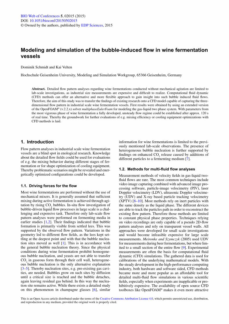
2.4. Validation simulationsWith different combinations of interfacial forces models multiple validation simulations were carried out to find the best fit to experimental data. Therefore results from bub-ble column investigations of Deen et al. (2001) were used [18]. Applying the drag model of Dijkhuizen et al. (2010) with a swarm correction coefficient from Roghair et al. (2013) in combination with the Rastello et al. (2011) lift model gave the best fit (see Fig. 1) [20–22].

Figure 1. Comparison of gas (g) and liquid (l) velocity component in y-direction from CFD simulation (Sim) with experimental data (Exp) collected by Deen et al. (2001) over a center line at y = 0.25 m.

BIO Web of Conferences

for measurements during beer fermentations, but where limited to a small section of the entire flow [9]. Experimental measurements are often the basis for computational fluid dynamic (CFD) simulations. The gathered data is used for calibrations of the underlying mathematical models. With the steady development in the high-performance computing industry, both hardware and software sided, CFD methods became more and more popular as an affordable tool for detailed multi-fluid flow simulations in various scientific fields, especially when experiments are inapplicable or prohibitively expensive. The availability of open source CFD toolboxes like OpenFOAM® makes it even more attractive for researchers, as the models can be further extended to best fit the specific conditions [11]. In addition CFD can be coupled with powerful optimization tool-kits (e.g. Dakota) to perform multiple, target-aimed experiments to find ideal configurations for a given problem [12].

The aim of this study was to transfer the findings of existing research onto a CFD model capable of capturing the three-dimensional flow pattern in industrial scale wine fermentation vessels. This model might then be used for further analyses of e.g. nutrient mixing evaluations or energy optimization studies.

2 Materials and methods

Under the premise of using free of charge open-source software OpenFOAM® (v.2.2.x)soon emerges as the predominant platform for CFD applications. For the necessary pre-processing, which includes geometry construction and meshing, Salome (v.7.4.0) [13] and snappyHexMesh, supplied with OpenFOAM®, were used. Data visualization was realized with the open-source post-processing application ParaView (v.4.1.0) [14].

2.1 Solver selection

To be able to simulate two-fluid flow processes, like the bubble induced flow during active wine fermentation, a suitable solver needed to be found. In general, three methods are available for that task: the Euler-Euler phase model, the Volume-of-Fluid (VOF) method and the Lagrangian particle tracking method [15]. While the latter ones are both able to resolve every single particle or bubble the Eulerian approach defines phases as interpenetrating continua. For a gas–liquid two phase case this means the definition of a continuous (liquid) and a dispersed phase (gas), which are represented by their phase fraction (α).

In industrial scale wine fermentation tank volumes of multiple cubic-meters are in use. For each cubic-meter of must approx. 50 m3 of CO2 is formed. The majority of this CO2 is released during fermentation as gas bubbles rising to the surface with diameters in the range of 0.05–5 mm [1, 16]. Hence, about 10 × 1010 bubbles/m3 must are created. On these grounds and with the current computational resources it would be impossible to model every single bubble on its own. Therefore only the Eulerian approach is feasible of modelling large-scale bubbly flows. With

twoPhaseEulerFoamandmultiphaseEulerFoamOpenFOAM® offers solvers including the Euler-Euler phase model. Our choice for using the incompressible, multiphase variant, recently developed by Wardle and Weller (2013), is based on the possibility to include additional phases in further studies and the option to switch on a VOF method for sharp interface capturing between specific phase pairs [17]. Turbulence is accounted for by a mixture Smagorinsky Large-Eddy-Simulation (LES) model [17]. LES models proved to be advantageous over Reynolds-Average turbulence models (RANS) in modeling bubbly two phase flows [18].

2.2 Governing equations

The applied solver is based on a set of mass and momentum equations (see eq. 1 and 2) for each phase k:

����� � ����� � � (1)

����������� � ������� � ����

� ���� � ���������� � ����g� ��

(2)

[17]

This system of partial-differential equations, derived from the incompressible, isothermalNavier-Stokes equations, is solved numerically by OpenFOAM®, as no analytical solution exists. Considering only two phases in this study, gas (g) and liquid (l), we have � ��g, l�.Applying gravity (g) is indispensable for multi-fluid CFD models.

2.3 Phase properties and coupling

Besides the representation by phase fractions, each phase is defined through its own thermo-physical properties (density (ρ), viscosity (µ), surface tension (σ)). In the standard configuration of the solver bubbles are modeled with a fixed bubble diameter (dB), which is applied to the dispersed phase (here CO2). To account for phase interactions, coupling between the phases is achieved by an interfacial forces source term (Fk), summing up all applied forces models. Therefore the basic solver already was set up with models for the drag and the virtual mass force. Multiple previous investigations of bubble flow have shown that the implementation of a lift force model could be advantageous for the representation of the transient bubble plume movement [18, 19]. Thus various lift force model formulations from literature were implemented in the solver, as well as additional drag force models.

2.4 Validation simulations

With different combinations of interfacial forces models

BIO Web of Conferences

for measurements during beer fermentations, but where limited to a small section of the entire flow [9]. Experimental measurements are often the basis for computational fluid dynamic (CFD) simulations. The gathered data is used for calibrations of the underlying mathematical models. With the steady development in the high-performance computing industry, both hardware and software sided, CFD methods became more and more popular as an affordable tool for detailed multi-fluid flow simulations in various scientific fields, especially when experiments are inapplicable or prohibitively expensive. The availability of open source CFD toolboxes like OpenFOAM® makes it even more attractive for researchers, as the models can be further extended to best fit the specific conditions [11]. In addition CFD can be coupled with powerful optimization tool-kits (e.g. Dakota) to perform multiple, target-aimed experiments to find ideal configurations for a given problem [12].

The aim of this study was to transfer the findings of existing research onto a CFD model capable of capturing the three-dimensional flow pattern in industrial scale wine fermentation vessels. This model might then be used for further analyses of e.g. nutrient mixing evaluations or energy optimization studies.

2 Materials and methods

Under the premise of using free of charge open-source software OpenFOAM® (v.2.2.x)soon emerges as the predominant platform for CFD applications. For the necessary pre-processing, which includes geometry construction and meshing, Salome (v.7.4.0) [13] and snappyHexMesh, supplied with OpenFOAM®, were used. Data visualization was realized with the open-source post-processing application ParaView (v.4.1.0) [14].

2.1 Solver selection

To be able to simulate two-fluid flow processes, like the bubble induced flow during active wine fermentation, a suitable solver needed to be found. In general, three methods are available for that task: the Euler-Euler phase model, the Volume-of-Fluid (VOF) method and the Lagrangian particle tracking method [15]. While the latter ones are both able to resolve every single particle or bubble the Eulerian approach defines phases as interpenetrating continua. For a gas–liquid two phase case this means the definition of a continuous (liquid) and a dispersed phase (gas), which are represented by their phase fraction (α).

In industrial scale wine fermentation tank volumes of multiple cubic-meters are in use. For each cubic-meter of must approx. 50 m3 of CO2 is formed. The majority of this CO2 is released during fermentation as gas bubbles rising to the surface with diameters in the range of 0.05–5 mm [1, 16]. Hence, about 10 × 1010 bubbles/m3 must are created. On these grounds and with the current computational resources it would be impossible to model every single bubble on its own. Therefore only the Eulerian approach is feasible of modelling large-scale bubbly flows. With

twoPhaseEulerFoamandmultiphaseEulerFoamOpenFOAM® offers solvers including the Euler-Euler phase model. Our choice for using the incompressible, multiphase variant, recently developed by Wardle and Weller (2013), is based on the possibility to include additional phases in further studies and the option to switch on a VOF method for sharp interface capturing between specific phase pairs [17]. Turbulence is accounted for by a mixture Smagorinsky Large-Eddy-Simulation (LES) model [17]. LES models proved to be advantageous over Reynolds-Average turbulence models (RANS) in modeling bubbly two phase flows [18].

2.2 Governing equations

The applied solver is based on a set of mass and momentum equations (see eq. 1 and 2) for each phase k:

����� � ����� � � (1)

����������� � ������� � ����

� ���� � ���������� � ����g� ��

(2)

[17]

This system of partial-differential equations, derived from the incompressible, isothermalNavier-Stokes equations, is solved numerically by OpenFOAM®, as no analytical solution exists. Considering only two phases in this study, gas (g) and liquid (l), we have � ��g, l�.Applying gravity (g) is indispensable for multi-fluid CFD models.

2.3 Phase properties and coupling

Besides the representation by phase fractions, each phase is defined through its own thermo-physical properties (density (ρ), viscosity (µ), surface tension (σ)). In the standard configuration of the solver bubbles are modeled with a fixed bubble diameter (dB), which is applied to the dispersed phase (here CO2). To account for phase interactions, coupling between the phases is achieved by an interfacial forces source term (Fk), summing up all applied forces models. Therefore the basic solver already was set up with models for the drag and the virtual mass force. Multiple previous investigations of bubble flow have shown that the implementation of a lift force model could be advantageous for the representation of the transient bubble plume movement [18, 19]. Thus various lift force model formulations from literature were implemented in the solver, as well as additional drag force models.

2.4 Validation simulations

With different combinations of interfacial forces models

BIO Web of Conferences

for measurements during beer fermentations, but where limited to a small section of the entire flow [9]. Experimental measurements are often the basis for computational fluid dynamic (CFD) simulations. The gathered data is used for calibrations of the underlying mathematical models. With the steady development in the high-performance computing industry, both hardware and software sided, CFD methods became more and more popular as an affordable tool for detailed multi-fluid flow simulations in various scientific fields, especially when experiments are inapplicable or prohibitively expensive. The availability of open source CFD toolboxes like OpenFOAM® makes it even more attractive for researchers, as the models can be further extended to best fit the specific conditions [11]. In addition CFD can be coupled with powerful optimization tool-kits (e.g. Dakota) to perform multiple, target-aimed experiments to find ideal configurations for a given problem [12].

The aim of this study was to transfer the findings of existing research onto a CFD model capable of capturing the three-dimensional flow pattern in industrial scale wine fermentation vessels. This model might then be used for further analyses of e.g. nutrient mixing evaluations or energy optimization studies.

2 Materials and methods

Under the premise of using free of charge open-source software OpenFOAM® (v.2.2.x)soon emerges as the predominant platform for CFD applications. For the necessary pre-processing, which includes geometry construction and meshing, Salome (v.7.4.0) [13] and snappyHexMesh, supplied with OpenFOAM®, were used. Data visualization was realized with the open-source post-processing application ParaView (v.4.1.0) [14].

2.1 Solver selection

To be able to simulate two-fluid flow processes, like the bubble induced flow during active wine fermentation, a suitable solver needed to be found. In general, three methods are available for that task: the Euler-Euler phase model, the Volume-of-Fluid (VOF) method and the Lagrangian particle tracking method [15]. While the latter ones are both able to resolve every single particle or bubble the Eulerian approach defines phases as interpenetrating continua. For a gas–liquid two phase case this means the definition of a continuous (liquid) and a dispersed phase (gas), which are represented by their phase fraction (α).

In industrial scale wine fermentation tank volumes of multiple cubic-meters are in use. For each cubic-meter of must approx. 50 m3 of CO2 is formed. The majority of this CO2 is released during fermentation as gas bubbles rising to the surface with diameters in the range of 0.05–5 mm [1, 16]. Hence, about 10 × 1010 bubbles/m3 must are created. On these grounds and with the current computational resources it would be impossible to model every single bubble on its own. Therefore only the Eulerian approach is feasible of modelling large-scale bubbly flows. With

twoPhaseEulerFoamandmultiphaseEulerFoamOpenFOAM® offers solvers including the Euler-Euler phase model. Our choice for using the incompressible, multiphase variant, recently developed by Wardle and Weller (2013), is based on the possibility to include additional phases in further studies and the option to switch on a VOF method for sharp interface capturing between specific phase pairs [17]. Turbulence is accounted for by a mixture Smagorinsky Large-Eddy-Simulation (LES) model [17]. LES models proved to be advantageous over Reynolds-Average turbulence models (RANS) in modeling bubbly two phase flows [18].

2.2 Governing equations

The applied solver is based on a set of mass and momentum equations (see eq. 1 and 2) for each phase k:

����� � ����� � � (1)

����������� � ������� � ����

� ���� � ���������� � ����g� ��

(2)

[17]

This system of partial-differential equations, derived from the incompressible, isothermalNavier-Stokes equations, is solved numerically by OpenFOAM®, as no analytical solution exists. Considering only two phases in this study, gas (g) and liquid (l), we have � ��g, l�.Applying gravity (g) is indispensable for multi-fluid CFD models.

2.3 Phase properties and coupling

Besides the representation by phase fractions, each phase is defined through its own thermo-physical properties (density (ρ), viscosity (µ), surface tension (σ)). In the standard configuration of the solver bubbles are modeled with a fixed bubble diameter (dB), which is applied to the dispersed phase (here CO2). To account for phase interactions, coupling between the phases is achieved by an interfacial forces source term (Fk), summing up all applied forces models. Therefore the basic solver already was set up with models for the drag and the virtual mass force. Multiple previous investigations of bubble flow have shown that the implementation of a lift force model could be advantageous for the representation of the transient bubble plume movement [18, 19]. Thus various lift force model formulations from literature were implemented in the solver, as well as additional drag force models.

2.4 Validation simulations

With different combinations of interfacial forces models

BIO Web of Conferences

for measurements during beer fermentations, but where limited to a small section of the entire flow [9]. Experimental measurements are often the basis for computational fluid dynamic (CFD) simulations. The gathered data is used for calibrations of the underlying mathematical models. With the steady development in the high-performance computing industry, both hardware and software sided, CFD methods became more and more popular as an affordable tool for detailed multi-fluid flow simulations in various scientific fields, especially when experiments are inapplicable or prohibitively expensive. The availability of open source CFD toolboxes like OpenFOAM® makes it even more attractive for researchers, as the models can be further extended to best fit the specific conditions [11]. In addition CFD can be coupled with powerful optimization tool-kits (e.g. Dakota) to perform multiple, target-aimed experiments to find ideal configurations for a given problem [12].

The aim of this study was to transfer the findings of existing research onto a CFD model capable of capturing the three-dimensional flow pattern in industrial scale wine fermentation vessels. This model might then be used for further analyses of e.g. nutrient mixing evaluations or energy optimization studies.

2 Materials and methods

Under the premise of using free of charge open-source software OpenFOAM® (v.2.2.x)soon emerges as the predominant platform for CFD applications. For the necessary pre-processing, which includes geometry construction and meshing, Salome (v.7.4.0) [13] and snappyHexMesh, supplied with OpenFOAM®, were used. Data visualization was realized with the open-source post-processing application ParaView (v.4.1.0) [14].

2.1 Solver selection

To be able to simulate two-fluid flow processes, like the bubble induced flow during active wine fermentation, a suitable solver needed to be found. In general, three methods are available for that task: the Euler-Euler phase model, the Volume-of-Fluid (VOF) method and the Lagrangian particle tracking method [15]. While the latter ones are both able to resolve every single particle or bubble the Eulerian approach defines phases as interpenetrating continua. For a gas–liquid two phase case this means the definition of a continuous (liquid) and a dispersed phase (gas), which are represented by their phase fraction (α).

In industrial scale wine fermentation tank volumes of multiple cubic-meters are in use. For each cubic-meter of must approx. 50 m3 of CO2 is formed. The majority of this CO2 is released during fermentation as gas bubbles rising to the surface with diameters in the range of 0.05–5 mm [1, 16]. Hence, about 10 × 1010 bubbles/m3 must are created. On these grounds and with the current computational resources it would be impossible to model every single bubble on its own. Therefore only the Eulerian approach is feasible of modelling large-scale bubbly flows. With

twoPhaseEulerFoamandmultiphaseEulerFoamOpenFOAM® offers solvers including the Euler-Euler phase model. Our choice for using the incompressible, multiphase variant, recently developed by Wardle and Weller (2013), is based on the possibility to include additional phases in further studies and the option to switch on a VOF method for sharp interface capturing between specific phase pairs [17]. Turbulence is accounted for by a mixture Smagorinsky Large-Eddy-Simulation (LES) model [17]. LES models proved to be advantageous over Reynolds-Average turbulence models (RANS) in modeling bubbly two phase flows [18].

2.2 Governing equations

The applied solver is based on a set of mass and momentum equations (see eq. 1 and 2) for each phase k:

����� � ����� � � (1)

����������� � ������� � ����

� ���� � ���������� � ����g� ��

(2)

[17]

This system of partial-differential equations, derived from the incompressible, isothermalNavier-Stokes equations, is solved numerically by OpenFOAM®, as no analytical solution exists. Considering only two phases in this study, gas (g) and liquid (l), we have � ��g, l�.Applying gravity (g) is indispensable for multi-fluid CFD models.

2.3 Phase properties and coupling

Besides the representation by phase fractions, each phase is defined through its own thermo-physical properties (density (ρ), viscosity (µ), surface tension (σ)). In the standard configuration of the solver bubbles are modeled with a fixed bubble diameter (dB), which is applied to the dispersed phase (here CO2). To account for phase interactions, coupling between the phases is achieved by an interfacial forces source term (Fk), summing up all applied forces models. Therefore the basic solver already was set up with models for the drag and the virtual mass force. Multiple previous investigations of bubble flow have shown that the implementation of a lift force model could be advantageous for the representation of the transient bubble plume movement [18, 19]. Thus various lift force model formulations from literature were implemented in the solver, as well as additional drag force models.

2.4 Validation simulations

With different combinations of interfacial forces models

BIO Web of Conferences

for measurements during beer fermentations, but where limited to a small section of the entire flow [9]. Experimental measurements are often the basis for computational fluid dynamic (CFD) simulations. The gathered data is used for calibrations of the underlying mathematical models. With the steady development in the high-performance computing industry, both hardware and software sided, CFD methods became more and more popular as an affordable tool for detailed multi-fluid flow simulations in various scientific fields, especially when experiments are inapplicable or prohibitively expensive. The availability of open source CFD toolboxes like OpenFOAM® makes it even more attractive for researchers, as the models can be further extended to best fit the specific conditions [11]. In addition CFD can be coupled with powerful optimization tool-kits (e.g. Dakota) to perform multiple, target-aimed experiments to find ideal configurations for a given problem [12].

The aim of this study was to transfer the findings of existing research onto a CFD model capable of capturing the three-dimensional flow pattern in industrial scale wine fermentation vessels. This model might then be used for further analyses of e.g. nutrient mixing evaluations or energy optimization studies.

2 Materials and methods

Under the premise of using free of charge open-source software OpenFOAM® (v.2.2.x)soon emerges as the predominant platform for CFD applications. For the necessary pre-processing, which includes geometry construction and meshing, Salome (v.7.4.0) [13] and snappyHexMesh, supplied with OpenFOAM®, were used. Data visualization was realized with the open-source post-processing application ParaView (v.4.1.0) [14].

2.1 Solver selection

To be able to simulate two-fluid flow processes, like the bubble induced flow during active wine fermentation, a suitable solver needed to be found. In general, three methods are available for that task: the Euler-Euler phase model, the Volume-of-Fluid (VOF) method and the Lagrangian particle tracking method [15]. While the latter ones are both able to resolve every single particle or bubble the Eulerian approach defines phases as interpenetrating continua. For a gas–liquid two phase case this means the definition of a continuous (liquid) and a dispersed phase (gas), which are represented by their phase fraction (α).

In industrial scale wine fermentation tank volumes of multiple cubic-meters are in use. For each cubic-meter of must approx. 50 m3 of CO2 is formed. The majority of this CO2 is released during fermentation as gas bubbles rising to the surface with diameters in the range of 0.05–5 mm [1, 16]. Hence, about 10 × 1010 bubbles/m3 must are created. On these grounds and with the current computational resources it would be impossible to model every single bubble on its own. Therefore only the Eulerian approach is feasible of modelling large-scale bubbly flows. With

twoPhaseEulerFoamandmultiphaseEulerFoamOpenFOAM® offers solvers including the Euler-Euler phase model. Our choice for using the incompressible, multiphase variant, recently developed by Wardle and Weller (2013), is based on the possibility to include additional phases in further studies and the option to switch on a VOF method for sharp interface capturing between specific phase pairs [17]. Turbulence is accounted for by a mixture Smagorinsky Large-Eddy-Simulation (LES) model [17]. LES models proved to be advantageous over Reynolds-Average turbulence models (RANS) in modeling bubbly two phase flows [18].

2.2 Governing equations

The applied solver is based on a set of mass and momentum equations (see eq. 1 and 2) for each phase k:

����� � ����� � � (1)

����������� � ������� � ����

� ���� � ���������� � ����g� ��

(2)

[17]

This system of partial-differential equations, derived from the incompressible, isothermalNavier-Stokes equations, is solved numerically by OpenFOAM®, as no analytical solution exists. Considering only two phases in this study, gas (g) and liquid (l), we have � ��g, l�.Applying gravity (g) is indispensable for multi-fluid CFD models.

2.3 Phase properties and coupling

Besides the representation by phase fractions, each phase is defined through its own thermo-physical properties (density (ρ), viscosity (µ), surface tension (σ)). In the standard configuration of the solver bubbles are modeled with a fixed bubble diameter (dB), which is applied to the dispersed phase (here CO2). To account for phase interactions, coupling between the phases is achieved by an interfacial forces source term (Fk), summing up all applied forces models. Therefore the basic solver already was set up with models for the drag and the virtual mass force. Multiple previous investigations of bubble flow have shown that the implementation of a lift force model could be advantageous for the representation of the transient bubble plume movement [18, 19]. Thus various lift force model formulations from literature were implemented in the solver, as well as additional drag force models.

2.4 Validation simulations

With different combinations of interfacial forces models

38th World Congress of Vine and Wine

02015-p.3

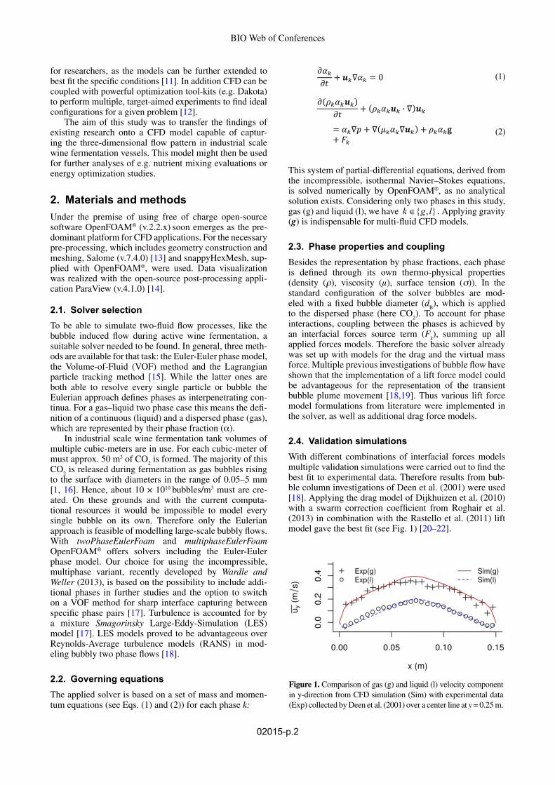
2.5. Wine fermentation – case setupIn our first approaches of wine fermentation simulations var-ious common vessel shapes were under consideration. In this paper we focus solely on a cylindrical tank with an approxi-mation of the widely used Kloepper head (GK) (see Fig. 2).

The final three-dimensional mesh for GK with a total volume of 11.15 m3 consisted of 412.808 cells, predomi-nantly of hexagonal shape.

Based on the observations in previous studies it was assumed that all bubble formation takes places at the bot-tom of the vessel and is induced by settled lees particles. Therefore by filling the geometry with a lees volume of 50 L a new bottom surface was defined, acting as the bub-ble formation zone (inlet) in the simulations. The specified volume is derived from the recommended residual lees content of 0.6 kg/kg must for a standard white wine fer-mentation [23]. Following this procedure the must fill level was set to match a total volume of 10 m3.

At the inlet surface a volumetric gas flow rate (Qg) of

1.5151515 × 10–3 m3/s was applied, equaling a CO2 gas for-

mation of 1 g/l/h that can be found during phases of high

fermentation activity [24]. All other relevant fluid and model parameters were set according to literature data (see Table 1).

2.6. ImplementationThe scientific Linux operating system Gm.Linux (v3.01) [30] was used on a work station equipped with an Intel® Xeon® E5-1620v2 processor and 32GB RAM. With that set-up 10 min of computational time were needed for the simulation of one second of real time. An automatic time-stepping approach, with a Courant number limit of 0.5, was used to assure accurate solutions [31].

3. Results and discussionThe following results of the flow pattern analyses are lim-ited to the liquid dominant zone inside the vessel, as that defines the area of interest for further investigations.

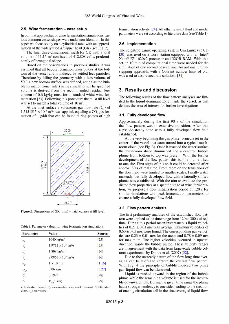
3.1. Fully developed flowApproximately during the first 90 s of the simulation the flow pattern was in extensive transition. After that a pseudo-steady state with a fully developed flow field established.

At the very beginning the gas phase formed a jet in the center of the vessel that soon turned into a typical mush-room cloud (see Fig. 3). Once it reached the water surface the mushroom shape diminished and a centered bubble plume from bottom to top was present. With the further development of the flow pattern this bubble plume tilted to one site. First signs of this shift could be detected after approx. 80 s of real time. From there on the transitions of the flow field were limited to smaller scales. Finally a still unsteady, but fully developed flow with a laterally shifted plume was established. With the aim to evaluate the pre-dicted flow properties at a specific stage of wine fermenta-tion, we propose a flow initialization period of 120 s for similar simulations with peak fermentation parameters, to ensure a fully developed flow field.

3.2. Flow pattern analysisThe first preliminary analyses of the established flow pat-tern were applied to the time range from 120 to 300 s of real time. During this period mean instantaneous liquid veloci-ties of 0.21 ± 0.01 m/s with average maximum velocities of 0.60 ± 0.05 m/s were found. The corresponding gas veloci-ties are 0.23 ± 0.01 m/s for the mean and 0.78 ± 0.09 m/s for maximum. The higher velocities occurred in upward direction, inside the bubble plume. These velocity ranges are in agreement with the data from large-scale bubble col-umn experiments by Dhotre et al. (2007) [32].

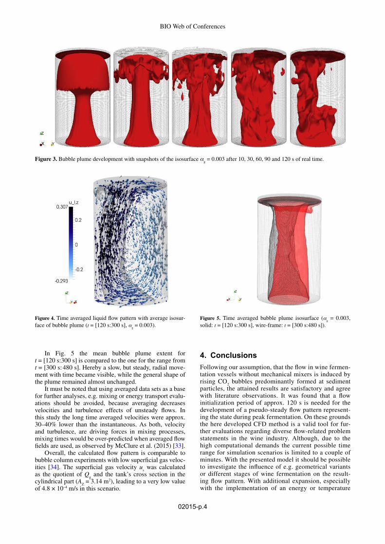
Due to the unsteady nature of the flow long time aver-aging can be useful to capture the overall flow pattern. With Fig. 4 the principle of bubble induced two phase gas–liquid flow can be illustrated.

Liquid is pushed upward in the region of the bubble plume while the remaining volume is used for the inevita-ble downward flow. During the given time range the plume had a stronger tendency to one side, leading to the creation of one big circulation cell in the time averaged liquid flow.

Figure 2. Dimensions of GK (mm) – hatched area

38th World Congress of Vine and Wine and 13th General Assembly of the OIV

multiple validation simulations were carried out to find the best fit to experimental data. Therefore results from bubble column investigations of Deen et al. (2001) were used [18]. Applying the drag model of Dijkhuizen et al. (2010) with a swarm correction coefficient from Roghair et al. (2013) in combination with the Rastello et al. (2011) lift model gave the best fit (see fig. 1) [20-22].

Figure 1. Comparison of gas (g) and liquid (l) velocity component in y-direction from CFD simulation (Sim) with experimental data (Exp) collected by Deen et al. (2001) over a center line at y=0.25 m

2.5 Wine fermentation — case setup

In our first approaches of wine fermentation simulations various common vessel shapes were under consideration. In this paper we focus solely on a cylindrical tank with an approximation of the widely used Kloepper head (GK) (see fig. 2).

Figure 2. Dimensions of GK (mm) – hatched area fill level

The final three-dimensional mesh for GK with a total volume of 11.15 m3 consisted of 412.808 cells, predominantly of hexagonal shape.

Based on the observations in previous studies it was assumed that all bubble formation takes places at the bottom of the vessel and is induced by settled lees particles. Therefore by filling the geometry with a lees volume of 50 L a new bottom surface was defined, acting as the bubble formation zone (inlet) in the simulations. The specified volume is derived from the recommended

residual lees content of 0.6 kg/kg must for a standard white wine fermentation [23]. Following this procedure the must fill level was set to match a total volume of 10 m3.

At the inlet surface a volumetric gas flow rate (Qg) of 1.5151515 × 10-3 m3/s was applied, equaling a CO2 gas formation of 1 g/l/h that can be found during phases of high fermentation activity [24]. All other relevant fluid and model parameters were set according to literature data (see tab. 1).

Table 1. Parameter values for wine fermentation simulations

Parameter Value Source ρl 1040 kg/m3 [25] νl 1.9712 × 10-6 m2/s [25] ρg 1.808 kg/m3 [26] νg 8.0863 × 10-6 m2/s [26] dB 1 × 10-3 m [1, 16] σg,l 0.06 kg/s2 [5, 27] Cs 0.1995 [28] Δ Vcell

1/3 (m) [29] ν: kinematic viscosity, Cs: dimensionless Smagorinsky constant, Δ: LES filter-width, Vcell: cell volume

2.6 Implementation

The scientific Linux operating system Gm.Linux (v3.01)[30] was used on a work station equipped with an Intel® Xeon® E5-1620v2 processor and 32GB RAM. With that set-up 10 minutes of computational time were needed for the simulation of one second of real time. An automatic time-stepping approach, with a Courant number limit of 0.5, was used to assure accurate solutions [31].

3 Results and discussion

The following results of the flow pattern analyses are limited to the liquid dominant zone inside the vessel, as that defines the area of interest for further investigations.

3.1 Fully developed flow

Approximately during the first 90 s of the simulation the flow pattern was in extensive transition. After that a pseudo-steady state with a fully developed flow field established.

At the very beginning the gas phase formed a jet in the center of the vessel that soon turned into a typical mushroom cloud (see fig. 3). Once it reached the water surface the mushroom shape diminished and a centered bubble plume from bottom to top was present.With the further development of the flow pattern thisbubble plume tilted to one site. First signs of this shift could be detected after approx. 80 s of real time. From there on the transitions of the flow field were limited to smaller scales. Finally a still unsteady, but fully developed flow with a laterally shifted plume was established. With the aim to evaluate the predicted flow properties at a specific

fill level.

Table 1. Parameter values for wine fermentation simulations.

Parameter Value Source

ρl

1040 kg/m3 [25]

νl

1.9712 × 10–6 m2/s [25]

ρg

1.808 kg/m3 [26]

νg

8.0863 × 10–6 m2/s [26]

dB

1 × 10–3 m [1,16]

σg,l

0.06 kg/s2 [5,27]

Cs

0.1995 [28]

Δ Vcell

1/3 (m) [29]

ν: kinematic viscosity, Cs: dimensionless Smagorinsky constant, Δ: LES filter-

width, Vcell

: cell volume.

BIO Web of Conferences

02015-p.4

In Fig. 5 the mean bubble plume extent for t = [120 s:300 s] is compared to the one for the range from t = [300 s: 480 s]. Hereby a slow, but steady, radial move-ment with time became visible, while the general shape of the plume remained almost unchanged.

It must be noted that using averaged data sets as a base for further analyses, e.g. mixing or energy transport evalu-ations should be avoided, because averaging decreases velocities and turbulence effects of unsteady flows. In this study the long time averaged velocities were approx. 30–40% lower than the instantaneous. As both, velocity and turbulence, are driving forces in mixing processes, mixing times would be over-predicted when averaged flow fields are used, as observed by McClure et al. (2015) [33].

Overall, the calculated flow pattern is comparable to bubble column experiments with low superficial gas veloc-ities [34]. The superficial gas velocity u

s was calculated

as the quotient of Qg and the tank’s cross section in the

cylindrical part (AZ = 3.14 m2), leading to a very low value

of 4.8 × 10–4 m/s in this scenario.

4. ConclusionsFollowing our assumption, that the flow in wine fermen-tation vessels without mechanical mixers is induced by rising CO

2 bubbles predominantly formed at sediment

particles, the attained results are satisfactory and agree with literature observations. It was found that a flow initialization period of approx. 120 s is needed for the development of a pseudo-steady flow pattern represent-ing the state during peak fermentation. On these grounds the here developed CFD method is a valid tool for fur-ther evaluations regarding diverse flow-related problem statements in the wine industry. Although, due to the high computational demands the current possible time range for simulation scenarios is limited to a couple of minutes. With the presented model it should be possible to investigate the influence of e.g. geometrical variants or different stages of wine fermentation on the result-ing flow pattern. With additional expansion, especially with the implementation of an energy or temperature

Figure 4. Time averaged liquid flow pattern with average isosur-face of bubble plume (t = [120 s:300 s], α

g = 0.003).

Figure 5. Time averaged bubble plume isosurface (αg = 0.003,

solid: t = [120 s:300 s], wire-frame: t = [300 s:480 s]).

Figure 3. Bubble plume development with snapshots of the isosurface αg = 0.003 after 10, 30, 60, 90 and 120 s of real time.

38th World Congress of Vine and Wine

02015-p.5

transport equation, the analytical scope could be further extended. By coupling the OpenFOAM® solver with optimization software (e.g. Dakota) studies on energy optimization of cooling equipment are the goal of our further research.

This study was supported by a grant from the German Federal Ministry of Education and Research (BMBF, Germany) as part of the joint project “Robust energy optimization of fer-mentation processes for the production of biogas and wine (ROENOBIO)”.

References [1] J. Delente, C. Akin, E. Krabbe, K. Ladenburg,

Biotechnol. Bioeng., 11, 631–646 (1969) [2] M. Diaz, A.I. Garcia, L.A. Garcia, Biotechnol.

Bioeng., 51, 131–140 (1996) [3] S. Lubetkin, Chem. Soc. Rev., 24, 243–250 (1995) [4] S. Fischer, Blasenbildung von in Flüssigkeiten gelös-

ten Gasen (TU München, München, 2001) [5] G. Liger-Belair, M. Parmentier, P. Jeandet,

J. Phys. Chem. B, 110, 21145–21151 (2006) [6] G. Liger-Belair, M. Vignes-Adler, C. Voisin,

B. Robillard, P. Jeandet, Langmuir, 18, 1294–1301 (2002)

[7] F. Kühbeck, M. Müller, W. Back, T. Kurz, M. Krottenthaler, Enzyme Microb. Technol., 41, 711–720 (2007)

[8] W. Nitsche, A. Brunn, Strömungsmesstechnik (Springer Science+Business Media, Berlin, 2006)

[9] H. Meironke, J.A. Szymczyk, Proc. Appl. Math. Mech., 5, 577–578 (2006)

[10] A.Seeger, K. Affeld, L. Goubergrits, U. Kertzscher, E. Wellnhofer, E. Exp. Fluids, 31, 193–201 (2001)

[11] H. Jasak, Int. J. Nav. Arch. Ocean Eng., 1, 89–94 (2009)

[12] B.M. Adams, M.S. Ebeida, M.S. Eldred, J.D. Jakeman, L.P. Swiler, A. Stephens, D.M. Vigil, T.M. Wildey, Sandia Technical Report SAND2014-4633 (Sandia National Laboratories, New Mexico, 2014)

[13] V. Bergeaud, V.V. Lefebvre, Proceedings of SNA + MC2010: Joint international conference on super-computing in nuclear applications (2010)

[14] U. Ayachit, The ParaView Guide: A Parallel Visualization Application (Kitware Inc., New York, 2015)

[15] Fluent, FLUENT 6.1 User’s Guide (Fluent Inc., 2003)

[16] A. Lübbert, T. Paaschen, A. Lapin, Biotechnol. Bioeng., 52, 248–258 (1996)

[17] K.E. Wardle, H.G. Weller, Int. J. Chem. Eng., 2013, Article ID 128936, 13 pages (2013)

[18] N. Deen, T. Solberg, B. Hjertager, B. Chem. Eng. Sci., 56, 6341–6349 (2001)

[19] H. Marschall, R. Mornhinweg, A. Kossmann, S. Oberhauser, K. Langbein, O. Hinrichsen, Chem. Eng. Technol., 34, 1311–1320 (2011)

[20] W. Dijkhuizen, I. Roghair, M. van Sint Annaland, J.A.M. Kuipers, Chem. Eng. Sci., 65, 1415–1426 (2010)

[21] I. Roghair, M. van Sint Annaland, J.A.M. Kuipers, AIChE J., 59, 1791–1800 (2013)

[22] M. Rastello, J.-L. Marié M. Lance, J Fluid Mech., 682, 434-459 (2011)

[23] J. Seckler, R. Jung, M. Freund, Vergleich alternati-ver Klärverfahren bei Most: (absitzen, separieren, flotieren, schönen), (ATW–KTBL, Darmstadt, 2000)

[24] M. Bely, J.-M. Sablayrolles, P. Barre, J. Ferment. Bioeng., 70, 246–252 (1990)

[25] R. Boulton, V. Singleton, L. Bisson, R. Kunkee, In: Principles and Practices of Winemaking, 492–520 (Springer, New York, 1999)

[26] F.J. McQuillan, J.R. Culham, M.M. Yovanovich, Microelectronics Heat Transfer Laboratory Report UW/MHTL 8407 G-02 (University of Waterloo, Waterloo, 1984)

[27] M. López-Barajas, A. Viu-Marco, E. López-Tamames, S. Buxaderas, M.C. de la Torre-Boronat, M. C., J. Agri. Food Chem., 45, 2526–2529 (1997)

[28] R.S. Rogallo, P. Moin, Annu. Rev. Fluid Mech., 16, 99–137 (1984)

[29] J.W. Deardorff, J. Fluid Mech., 41, 453–480 (1970)[30] M. Günther, K. Velten, Mathematische Modellbildung

und Simulation (Wiley-VCH, Berlin, 2014)[31] R. Courant, K. Friedrichs, H. Lewy, Math. Ann.,

100, 100, 32–74 (1928)[32] M.T. Dhotre, B.L. Smith, Chem. Eng. Sci., 62,

6615–6630 (2007)[33] D.D. McClure, N. Aboudha, J.M. Kavanagh,

D.F. Fletcher, G.W. Barton, Chem. Eng. J., 264, 291–301 (2015)

[34] M.E. Diaz, F.J. Montes, M.A. Galan, 2006 AIChE Annual Meeting Conference Proceedings (AIChE, New York, 2006)