1

Modeling and Simulation:

Tools for Metabolic Engineering

Wolfgang Wiechert

Institute of Mechanical and Control Engineering,

Dept. of Simulation and Computer Science

Paul-Bonatz-Str. 9-11

University of Siegen, D-57068 Siegen, Germany

Phone: –271-740-4727 Fax: -2365

E-Mail: wiechert@simtec.mb.uni-siegen.de

To appear in: Journal of Biotechnology (2001)

2

Abstract: Mathematical modeling is one of the key methodologies of metabolic engineering.

Based on a given metabolic model different computational tools for the simulation, data evalua-

tion, systems analysis, prediction, design and optimization of metabolic systems have been de-

veloped. The currently used metabolic modeling approaches can be subdivided into structural

models, stoichiometric models, carbon flux models, stationary and nonstationary mechanistic

models and models with gene regulation. However, the power of a model strongly depends on its

basic modeling assumptions, the simplifications made and the data sources used. Model valida-

tion turns out to be particularly difficult for metabolic systems. The different modeling ap-

proaches are critically reviewed with respect to their potential and benefits for the metabolic en-

gineering cycle. Several tools are discussed that have emerged from the different modeling ap-

proaches including structural pathway synthesis, stoichiometric pathway analysis, metabolic flux

analysis, metabolic control analysis, optimization of regulatory architectures and the evaluation

of rapid sampling experiments.

Keywords: Metabolic Engineering, Metabolic Modeling, Stoichiometry, Flux Analysis, Mecha-

nistic Models, Metabolic Optimization, Model Validation

3

Introduction

Modeling for Metabolic Engineering

The goal of metabolic engineering is the development of targeted methods to improve the meta-

bolic capabilities of industrially relevant microorganisms. In order to reach this ambitious goal

tools are required that assist in the evolutionary process of genetic manipulations of the cell me-

tabolism and the improvement of bioprocess conditions. From an engineering perspective mathe-

matical modeling is one of the most successful scientific tools available for this task. For techni-

cal systems the routine application of modeling and simulation software is already state of the art.

In certain fields as for instance the design of analog electrical circuits, these tools have already

reached a state of maturity that makes experiments and physical prototype development superflu-

ous.

The challenge now is to transfer and adapt the developed modeling methodology from technical

to biological systems. The question of the extent to which this is applicable remains open because

there are several substantial differences between the two worlds as will be shown in the follow-

ing. In particular, biological systems cannot be easily decomposed into unit components. How-

ever, our functional knowledge about cellular systems and the available database is growing dra-

matically. For this reason the present contribution surveys current progress in the modeling and

analysis of metabolic networks. Emphasis is laid on the critical evaluation of model validity, on

the classification of current models and methods, and on the application potential of model-based

tools.

Aims and Scope of Metabolic Models

Starting with the modeling process for a given complex system the aim of the model should be

specified and the task for which a model-based tool is intended to be developed. The following

typical aims can be identified. They are ordered by an increasing demand for the precision and

quality of the model:

4

1. Structural understanding: Mathematical models are the most precise representation of

knowledge because they have a unique and objective interpretation. Thus they do not permit

any vague statements. Consequently modeling can be considered as a method to structure our

often rather diffuse and entangled knowledge. Even if the model is not used for simulation

this can already help to focus the attention on what is considered to be the essential parts of

the system. In recent years this methodology has been extremely successful in the design of

complex software systems (Rumbaugh et al., 1997).

2. Exploratory simulation: Undoubtedly the most frequent application of models is the explo-

ration of the possible behavior of a system. Simulation scenarios based on rather crude

mathematical models can help to achieve a rough understanding of the system behavior and

to reject false hypotheses. Clearly, such speculative studies cannot directly help to produce

the right ideas. Nevertheless, they help to focus on the most probable explanations for the be-

havior of the metabolic system. Many conceptual studies based on more or less simple mod-

els belong to this category. Several interesting examples are presented in (Heinrich and

Schuster, 1996).

3. Interpretation and evaluation of measured data: The reproduction of experimental data by

mathematical models is a well established tool in all scientific disciplines. For example, the

characterization of growth, nutrient uptake and product formation by macrokinetic models

has become a standard procedure in bioprocess development (Takors et al., 1997). However,

it must be pointed out that in most cases this is merely a reproduction of the measured data.

Thus it cannot be concluded that the respective model is a “good” one or even that it has any

predictive power. Without further measures the fitting of models to data tends to produce a

consistent ”interpretation” rather than an “explanation” of the empirical results.

4. Systems analysis: Based on a given model mathematical methods can help to obtain a better

understanding of the system’s structure and its qualitative behavior. Of main interest are

methods for the identification of functional units in metabolic and genetic systems, for the

computation of stable states (Torres, 1994a), for the determination of parameter sensitivities

(Albe and Wright, 1992; Torres, 1994b), for investigating the dynamic behavior (Shiraishi

and Savageau, 1992), for explaining oscillating or even chaotic behavior (Goldbeter, 1996) or

5

for computing theoretical limits of the systems metabolic capabilities (Edwards and Palsson,

1998). However, a more or less correct and precise model is required to obtain meaningful re-

sults.

5. Prediction and design: Based on a validated model the outcome of future experiments can

be predicted. Clearly, the goal of this tool is the support of a rational design process for meta-

bolic pathways. However, as will become clear later the validity and predictive power of

metabolic models is often restricted to a narrow scope that does not always contain the in-

tended target configuration.

6. Optimization: Once models are available that are predictive, at least in some parameter re-

gion, the ultimate goal of modeling in metabolic engineering can be tackled which is the

computation of an optimal metabolic design (Hatzimanikatis et al., 1996). Such methods are

state of the art in engineering disciplines like mechanics, electronics or civil engineering (Es-

chenauer et al., 1990). However, things are different with biotechnological systems.

Closely related to the model aim is the definition of the model scope and the required accuracy.

The application of a model is always limited to a certain type of problem. For example, a stoichi-

ometric network model (see below) is suitable for metabolic flux analysis but it contains no in-

formation about regulatory mechanisms. Thus it has little predictive power with respect to path-

way alterations. Likewise model validation for regulatory models is usually done with measured

data from a few physiological states (e.g. exponential growth in a batch culture). If a prediction is

made outside this scope it must be treated with great care. Clearly, with respect to accuracy rough

models can only produce rough predictions.

In general the following should be specified for a metabolic model: i) parameter and concentra-

tion range in which it is validated, ii) external conditions and inputs for which it works and iii)

physiological modes for which it holds. As a rule, a model should always be as simple as possible

and as complex as necessary. Clearly, the complexity of a model will grow if its scope and accu-

racy is extended. Thus the requirements should always be as modest as possible with respect to

the problem to be solved.

6

Ingredients of a Metabolic Model

For any mathematical model several types of modeling assumptions and the data sources used

must be precisely documented in order to judge its applicability in a certain situation. The fol-

lowing aspects will later be discussed in more detail for each category of metabolic model:

1. Abstraction level: We are used to describing the complexity of cellular systems by different

types of abstractions like gene maps, metabolic reaction networks, enzyme reaction mecha-

nisms, geometric models, macromolecular structures and so on. Thus we focus on those cel-

lular components and processes that are of interest in the current investigation and neglect the

influence (and often even the presence) of all other parts. The basic abstraction of most meta-

bolic models is the system compartmentalization into a number of homogeneously distributed

pools connected by metabolic fluxes (Figure 1). The number of particles in each pool is so

large that its stochastic fluctuations can be neglected. A concentration variable is then used to

describe the state of the pool.

2. Modeling principles: Having chosen the level of abstraction the formulation of the model

equations is guided by general modeling principles. In the case of compartmental modeling

these are essentially the physical laws of mass and energy conservation. They lead directly to

a set of balance equations that describe the system dynamics or equilibrium. Having deter-

mined the fluxes and pools that should belong to the model this is a strictly formal process

and thus can be supported by modern modeling tools (Cellier, 1991).

3. Basic laws: One ingredient that is missing for the conversion of the balance equations into a

structurally fully specified model is the representation of all fluxes in terms of the system

state given by the vector of all metabolite concentrations. Usually the laws of enzyme kinetics

as obtained from in vitro experiments (Cornish-Bowden and Wharton, 1988) are assumed

also to hold in the intracellular environment.

4. Simplifying assumptions: Although a modeling framework might be capable of describing a

metabolic system in considerable detail the number of equations and parameters arising are

usually too large for a practical application of the model. For this reason simplifying assump-

7

tions are made to reduce the model complexity. Frequently encountered assumptions are the

lumping together of metabolite pools or the condensation of whole pathways into some few

reaction steps (Vallino, 1991). If simplification is carefully done it seldom restricts the in-

tended scope of the model.

5. Kinetic parameters used: When the kinetic laws are filled into the model it is almost ready

for simulation. However, the kinetic constants are still missing. They are usually taken from

the literature or available data-bases (Schomburg, 1997). Nevertheless, great care must be

taken in this operation because the published constants were produced with different organ-

isms and strains, different experimental and measurement methods and different evaluation

approaches (Ewings and Doelle, 1980).

6. Measured data used: The most critical ingredient of the modeling process is measured data

from the in vivo system. Clearly, complex metabolic models can only be validated with in

vivo data from the functioning system. Different measurement techniques are under devel-

opment to obtain a realistic picture of the functioning biological system. These are metabolic

flux analysis (Vallino and Stephanopoulos, 1993), rapid sampling (Theobald et al. 1997),

proteome analysis (Hatzimanikatis et al., 1999) or DNA chips (Derisi et al. 1997). They all

produce enormous amounts of data that complement the parameter set taken from databases.

Model Validation

Only models that are valid within their declared scope lead to successful tools. Unfortunately,

model validation is still the most difficult problem in the modeling process. It is already difficult

to define what a valid model is in a precise mathematical sense. The common definition of valid-

ity is that a model can predict all experiments within the scope of the model. This is nothing else

but a positive formulation of Popper’s falsification principle (Popper, 1971): a model is valid if it

resists all falsification attempts. The problem with this definition is that model validity can never

be proven because there will always be one more experiment to do. Thus a more pragmatic ap-

proach is required from which an experimental validation procedure can be derived. Such con-

8

cepts have been mainly developed in the statistical disciplines of regression analysis and experi-

mental design.

A qualitative concept of model validation can be used if the precision requirements of the model

are rather low. For many purposes it is then sufficient if the model is able to reproduce the basic

behavior of the real system (e.g. stability, bifurcations, oscillations etc.) sufficiently well. This

can be decided by methods from nonlinear systems theory.

A much stricter validation concept is derived from the falsification principle: if we cannot say

what a good model is let’s specify what a bad model is. Then try to find a model which explains

the data and withstands all attempts to reveal it weaknesses. Clearly, this does still not guarantee

a predictive model but it approximates this concept. The statistical procedure now is as follows:

take a certain model and assume its validity, then fit the model parameters to the given data and

apply a battery of statistical procedures to falsify the validity hypothesis. For example, all data

must be sufficiently well reproduced and all predictions must have reasonably small confidence

intervals (Seber and Wild, 1989).

An extension to this concept is model discrimination. In this case a family of differently struc-

tured models representing various possible explanation hypotheses for the function of the real

system compete for the best explanation of the data set (Linhart and Zucchini, 1986). In general,

the winner of this competition will be the “smallest” model that passes all statistical tests. Model

discrimination can be further extended to a discriminating experimental design process in which

further experiments are designed in order to discriminate between a family of models (Box and

Hill, 1967). By this approach missing information for model validation is successively produced

in a systematic way. It has been successfully applied to the discrimination of standard macroki-

netic process models (Takors et al., 1997).

9

Promises of Metabolic Modeling

It will become clear in the following that quite a lot of assumptions are required to build complex

models of biological systems. While the validity of basic physical laws like mass conservation is

indisputable and some biological assumptions like knowledge of the biochemical network are

generally accepted, other assumptions like that of a constant P/O ratio are highly speculative and

not well justified. Thus the predictive power of some types of metabolic models is currently not

very high.

It’s worthwhile comparing this situation with the state of the art in the design of technical sys-

tems. Electrical circuits are a good example because they have much in common with chemical

reaction networks. They are modeled on the basis of the abstraction of homogeneous electrical

fields and the modeling principle is the conservation of charge so that electrical current balances

resemble the metabolic flux balances (Cellier, 1991). The basic laws describe the behavior of

resistors, capacities, inductivities etc. Simplifying assumptions are frequently made to describe

active components like diodes or transistors or to neglect the effect of temperature.

The first big difference between electrical and metabolic systems is that in the electrical system

any component can be isolated from the system without affecting its function. Secondly, the

number of different component types (resistances, capacities, inductivities) in a circuit is quite

small so that a few elementary laws can be reused in many places of the system. Thirdly, all pos-

sible interactions between the system components are exactly known because they are precisely

given by the man-made circuit diagram. For these reasons it is state of the art in electrical circuit

design to replace the experiment by a simulation without casting any doubt on the accuracy of the

results.

Summarizing, the transfer of the modeling methodology from technical to biological processes is

a very ambitious task and at the current state of knowledge it is unlikely that quantitatively pre-

dictive models with a broad scope will be obtained. It is to be expected that genome research will

bring much greater functional knowledge about the biological system (Edwards and Palsson,

1998; Kao, 1999). Likewise in vivo measurement methods are under development that portray

10

the intracellular state of a living cell as completely and as reliably as possible. The great chal-

lenge is to link these data sources in order to get the complete picture.

On the other hand, if less ambitious goals are set for metabolic modeling there are already a

number of successful applications of modeling and system analysis. Some characteristic exam-

ples will be discussed in the next sections. The basic types of current modeling approaches in the

field of metabolic engineering can be classified as indicated by the following sections. They are

ordered by increasing mathematical complexity and requirement for model validation.

Focus of the present review

Mathematical models and simulation methods have been applied to cellular and metabolic sys-

tems for more than three decades and thus are not unique for metabolic engineering. The main

focus of modeling in cell physiology always was the understanding of metabolic systems in the

sense of the general principles which govern the cellular function. The new aspect of modeling in

metabolic engineering is the usage of models for the targeted direction of metabolic fluxes in the

sense of a rational engineering design.

Clearly, a thorough understanding of the complex metabolic regulation is always the best way to

achieve such improvements. However it is in principle not necessary to aim at a deep under-

standing. Many successful technical applications of black box models like for example linear

models or neural networks have proven the opposite. On the other hand models should always

incorporate as much secured knowledge about the biological system as possible while wrong or

uncertain assumptions might cause a loss of predictive power. Thus a major concern of the pres-

ent review is the critical discussion of model validity.

It is not surprising that there are several methodological differences between the „older“ cell

physiology community and the „younger“ metabolic engineering community. Only in recent

years a scientific interchange between both communities has begun and in particular the termi-

nology and the methods are translated if not unified. Interestingly this is no “one-way” relation

11

because the system design aspect has also consequences for the system understanding aspect

(Hofmeyer et al., 2000).

There are several excellent general introductions to metabolic engineering and certain of its as-

pects (Bailey, 1991; Stephanopoulos, Sinskey, 1993; Nielsen, 1998; Stephanopoulos, 1999).

Likewise there are two excellent textbooks from the cellular physiology viewpoint at the one

hand (Schuster, 1996) and the metabolic engineering viewpoint at the other hand (Stephanopou-

los et al., 1998). Both also cover mathematical tools. The new aspects of the present review now

is

- to develop a systematic framework by which current modeling activities can be classified and

judged,

- to bring together and compare results from cell physiology and metabolic engineering,

- to thoroughly discuss the aspect of model validity which is a crucial aspect for the application

of any model, and

- to emphasize the metabolic design aspect which sheds another light on the applicability of

classical tools from cell physiology.

The classification hopefully is a helpful guide for the reader into a vast amount of literature, al-

though it cannot cover any published modeling method. The review concentrates on publications

with a major focus on modeling and mathematical tools. Because this is a text about metabolic

engineering it primarily concentrates on the first decade of this discipline since about 1990. To

keep the number of citations reasonably low standard textbooks are preferred over the explicit

citation of articles from the seventies and eighties.

12

Structural Network Models

Basic assumptions

The biochemical structure of at least the central metabolic pathways is the only biological know-

ledge whose validity is (almost) undisputed. All chemical reaction steps are known, the reaction

mechanisms are well understood in most cases and also many cofactors and effectors are avail-

able from textbooks and databases (Michal, 1999; Kanehisa, 1999). On this basis, structural mod-

els of metabolism can be constructed which – in mathematical terminology – are represented by

bipartite directed graphs (Figure 2). This means that there are two types of nodes, i.e. flux nodes

and substance nodes. A flux node can only be connected to substance nodes and vice versa. The

role of the substances in a reaction step (e.g. as a substrate, product, cofactor or inhibitor) can be

further specified by annotating the arcs of the graph. There is no further need for parameters and

measurement data.

Developed tools

Inspired by the graphical representation, methods from graph theory, network theory, automata

theory or formal language theory can be applied. Typical results that can be achieved by these

methods are:

1. Pathway modeling: The first step to structural analysis must be the specification of the net-

work in some user-friendly way. Different textual and graphical tools have been developed to

generate a structural network description from the user input (Hofestädt, 1993).

2. Pathway synthesis: Physiologically meaningful biochemical pathways can be computed by

graph component analysis (Seressiotis and Bailey, 1988; Mavrovouniotis, 1992). They repre-

sent basic metabolic operation modes with a certain function. Likewise the discovery of

regulatory loops and signaling cascades is possible (Kohn and Lemieux, 1991).

3. Qualitative dynamic analysis: The network structure can also be interpreted by a Petri net.

Petri net tools can then be applied to analyze the network consistency and completeness in

13

terms of deadlocks or unreachable states (Reddy et al., 1993). Another dynamic description is

given by automata (Thomas, 1991).

4. Visualization tools: Flexible graphical network representations are urgently required to fa-

cilitate the interactive inspection of network structures and the visualization of all the quanti-

tative results produced by the subsequently described tools. However, the problem of auto-

matic graph drawing from a structural input is not that easy (Karp and Paley, 1994).

5. Optimal pathway synthesis: An application of structural methods that might be of interest in

the metabolic design of new pathways is the computation of optimal reaction networks which

produce certain product metabolites from given substrates. For example, the pentose phos-

phate pathway produces C3- and C4-molecules from C5-molecules without waste. This task

can be formulated as a combinatorial puzzle where generalized biochemical reaction steps

(e.g. group transfer reactions) have to be combined to reach the goal. Then the reaction ar-

chitecture is computed with a minimal number of reaction steps under certain thermodynamic

feasibility constraints. In the case of the pentose phosphate pathway it was shown that the

evolutionary solution to this problem is really optimal (Melendez-Hevia, 1994). However, if

this method is applied to new design problems it remains unclear whether a suggested path-

way constructed from generalized reaction steps is physically realizable by genetic engineer-

ing.

6. Functional genomics: While the discrete structure of the central metabolic pathways is rather

well understood our knowledge about the whole metabolism and about the genetic regulation

of enzyme expression is rather incomplete. In these areas the first goal must be to develop the

structural model (Collado-Vides, J., 1989; Hatzimanikatis et al., 1999). The challenge of

functional genomics is the unraveling of the regulatory network from known facts about gene

expression patterns that e.g. are produced with DNA chips and electrophoresis gels (Kao,

1999).

7. Thermodynamic and qualitative reasoning: ∆G0´ constants must be treated with care be-

cause they are not in general valid for the nonequilibrium situation (Westerhoff and van Dam,

1987). Consequently, ∆G0´ values may serve as a rather qualitative measure which imposes

14

further constraints on the model. Some qualitative tools which take thermodynamic or other

qualitative information into account are described in (Mavrovouniotis, 1993). The relation

between thermodynamics and kinetics is discussed in (Nielsen, 1997).

Stoichiometric Network Models

Basic assumptions and measured data

Structural models do not contain any quantitative information about substance concentrations or

metabolic fluxes. Thus structural methods can only detect possible regulatory structures but it

remains unanswered whether these regulation mechanisms are also quantitatively relevant in a

certain physiological state of the cells. In particular, if an enzyme is influenced by several an-

tagonistic cofactors and effectors in a nonlinear way (like e.g. phosphofructokinase) almost any-

thing can happen.

Most industrial production processes are operated under quasi-stationary conditions which means

that the main process parameters, i.e. substrate concentration, oxygen concentration, dilution rate

etc., are kept constant at least within time spans of about one hour. Because the regulatory time

constants of metabolic systems are much smaller it is usually assumed that stationary conditions

will also emerge in all metabolite pools of each single microbial cell. However, this is not neces-

sarily the case. Oscillations are quite frequent in biological systems (Goldbeter, 1996) and have

been observed in synchronized cultures. But the single cells may also fluctuate around a certain

state because there is a cell cycle. Then the overall impression of the cell population would be

that of a stationary system because the cell cycles are not synchronized. It is currently not known

how large this effect is. But even if each single cell had quasi-stationary pool sizes it might be the

case that different subpopulations have different flux patterns. Unfortunately, the development of

experimental single cell methods is only at the beginning and thus no data is available to quanti-

tate these effects. Summarizing, the assumption of quasi-stationarity is well justified for the time

average of a structured cell population. On the other hand, fluxes observed in a cell population

15

cannot in general be transferred to a single cell. Thus – if required – it must be postulated that this

transfer is possible.

If constant fluxes and intracellular pool sizes are assumed for the “average” cell the stoichiometry

of the metabolic network induces a set of linear relationships between the metabolic fluxes (Fig-

ure 2) which is generally expressed as

0vN =⋅ (1)

where N is the stoichiometric matrix and v is the vector of all metabolic fluxes. The stoichi-

ometric relations can be written for net fluxes as well as for separated forward and backward

fluxes (cf. Figure 5). The latter becomes necessary if both directions of bidirectional reactions

steps need to be formally considered as different reactions. An important difference between net

fluxes and forward/backward fluxes is that the latter must always be positive while the net flux –

as the difference of forward and backward flux – can have both signs.

A crucial simplification necessary for compartmental modeling in practice is the lumping of

pools. Usually, pools which are connected by rapidly exchanging reactions (e.g. the ribose-5-,

ribulose-5- and xylulose-5-phosphate pool in the pentose phosphate pathway) are lumped to-

gether into one single pool. Similarly, linear reaction sequences without any branch point (e.g.

the oxidative pentose phosphate pathway) can be lumped into a single reaction step (Vallino,

1991). However it must be taken care that only so called monofunctional units are considered as a

module (Rohwer et al., 1996).

Moreover, there are many reaction steps in complex metabolic models which are not modeled in

detail because they are assumed to be of minor importance. For example, all the anabolic reac-

tions outside the central metabolism cannot be modeled in detail (i.e. for each single step) be-

cause this would expand the model to an unmanageable size. Thus they are lumped together into

formal reaction steps. Non-integer stoichiometric constants may occur in this case because formal

pools like “cell mass”, “energy supply” or “organic acids” may be contained. A particularly im-

portant fact is that biomass is always composed of 12 elementary precursor metabolites (Neid-

hardt et al., 1990). The percentual precursor demand to synthetize the cell mass is assumed to be

constant under quite varying nutritional conditions (Vallino, 1991). This produces a very impor-

tant set of 12 noninteger coefficients.

16

A special problem is the intracellular compartmentalization of eucaryotes where reaction steps

are localized in a specific compartment. For example, the citric acid cycle takes place inside the

mitochondria. On the other hand there are some reactions that can be found in several compart-

ments and thus must be duplicated to obtain a correct network model. For example there are two

functioning glycolytic pathways in plant cells (Rees, 1988). The different compartments are

linked by transport steps over the intracellular membranes which have to be incorporated into the

flux model.

One of the most critical assumptions in stoichiometric modeling is the balancing of the “energy

metabolites” ATP, UTP, NADH, NADPH etc. To this end, the stoichiometric coefficients of

some very complex intracellular processes must be assumed. Firstly, the generation of ATP from

NADH and oxygen must be described by a P/O ratio which is usually around 2.5. However, there

is a continuing discussion about this ratio and its dependence on intracellular conditions (Brand,

1994; Fitton et al. 1994; Sauer and Bailey, 1999). Secondly, the ATP requirement for biomass

synthesis must be assumed. Thirdly, all processes producing and consuming the energy metabo-

lites must be known quantitatively. This makes energy balancing a rather doubtful procedure and

indeed flux analysis studies that do not rely on energy balancing (see below) showed that the en-

ergy balances are not closed (Marx et al., 1996).

Several metabolic fluxes can be directly measured. These are the “extracellular” fluxes like prod-

uct formation, oxygen uptake or carbon dioxide evolution and the growth rate. Additionally -

when a detailed chemical analysis of cell mass composition is available - the corresponding pre-

cursor demands can be directly computed from the growth rate (Vallino, 1991). This produces

another set of directly measured metabolic fluxes.

Developed tools

Having accepted the mentioned assumptions and simplifications, the stoichiometric model can be

used for different purposes. The key to all these tools is that the space of all possible flux patterns

v is strongly restricted by the stoichiometric relations to a low-dimensional linear subspace

17

(Schilling et al., 1999). In addition to the measurable precursor effluxes there typically remain

about 5 degrees of freedom for the central metabolic pathways of a procaryotic cell. The exploi-

tation of this linear flux space led to the development of some powerful tools:

1. Matrix generation: The key to all stoichiometric methods is the automatic generation of the

stoichiometric matrix N from a textual input in a familiar chemical reaction notation. Several

modeling tools have been developed (Vallino, 1991; Pfeiffer et al., 1999). Once the matrix

has been generated, subsequent methods are based on standard matrix calculations as are

readily available within scientific computing environments like MATLAB or MATHE-

MATICA.

2. Metabolic flux analysis: Stoichiometry-based MFA complements the stoichiometric rela-

tions by the measured fluxes. If the flux measurements are nonredundant and if not too many

degrees of freedom remain all intracellular metabolic fluxes can be estimated from the data

(Vallino and Stephanopoulos, 1993; Varma, Palsson, 1994). This turns out to be a classical

linear estimation exercise for which all relevant problems have been solved (Vallino, 1991;

Van Heijden et al., 1994a,b): the structural identifiability of the fluxes can be decided, all

fluxes can be efficiently computed, the available redundant information is fully used, a confi-

dence region for the estimated fluxes can be computed, the set of redundancy relations for the

measured data can be derived explicitly, and gross measurement errors can be detected. Thus

from a methodological viewpoint stoichiometry-based metabolic flux analysis is a mature tool

for metabolic engineering. However, without energy balancing the flux balances are usually

underdetermined.

3. Extreme flux patterns: Forward and backward fluxes are now considered separately in the

stoichiometric relations. Additionally some fluxes can be assumed to be unidirectional based

on thermodynamic considerations, i.e. the back flux is set to zero. If the substrate uptake is

scaled to one (i.e. 100%) the arising inequality 0v ≥ then further restricts the set of possible

flux patterns to a convex polyhedron in the flux space (Figure 3) (Clarke, 1988). Any point in

this polyhedron represents a feasible flux pattern of the system. The corner points of the

polyhedron - called the extreme points or the extreme flux patterns - are of special interest

18

because they exactly determine the feasible flux space. Algorithms for the calculation of ex-

treme points are available (Hohenbalken et al., 1987).

An extreme flux pattern is characterized by the fact that the number of fluxes which vanish in

this flux pattern is at a local maximum. Thus the extreme flux patterns can be interpreted as

basic metabolic operation modes where only some of the reaction steps are active (Figure 4).

Any other flux pattern can be represented by a weighted combination of the extreme flux

patterns. This gives an understanding of the metabolic network in terms of certain distinctive

physiologically patterns.

Optimal flux patterns: A rather speculative extension to the extreme point analysis is the

complementation of the stoichiometric relations by a linear metabolic optimization criterion.

Several criteria like maximal growth rate, maximal product formation or a minimal ATP pro-

duction for a given substrate uptake have been investigated (Edwards and Palsson, 1998).

They all lead to a classical linear programming problem which can be solved by the simplex

algorithm. Optimality criteria have also been used to solve the metabolic flux balances in the

case where the measured data (even with energy balancing) is still not sufficient to compute a

unique solution (Bonarius et al., 1997).

Except for degenerate cases the optimization result is always an extreme flux pattern. How-

ever, such a result need not represent a reasonable solution. For example the maximal lycine

production rate for C. glutamicum has been computed to more than 60% of the glucose up-

take rate in (Vallino, 1991) while current values from production processes are below 30%.

The difference comes from the fact that in order to reach maximal product formation the or-

ganism must stop any “waste” of energy for growth or maintenance.

4. Elementary flux modes: Extreme flux patterns are not always convincing solutions to the

problem of finding physiologically meaningful pathways in a metabolic network. Several ap-

proaches have been undertaken to obtain a biologically meaningful and yet mathematically

precise definition of a metabolic pathway. A recent definition of such elementary flux modes

requires that an elementary mode has a maximal number of vanishing fluxes and cannot be

decomposed into smaller pathways (Schuster et al., 1999). Thus elementary modes are the

19

smallest functioning subunits of a metabolic network. This motivates the hypothesis that they

are also genetically regulated as a unit which in turn is a promising approach to the develop-

ment of functional genomics tools. Elementary modes can be efficiently calculated by a

newly designed algorithm that has some similarity to the simplex algorithm (Pfeiffer et al.,

1999). They have several promising applications in metabolic design, drug development or

functional genomics (Schuster et al., 1999).

Carbon Flux Models

Basic assumptions and measured data

Stoichiometry-based flux analysis suffers from the disadvantage that the energy metabolites must

be balanced in detail, parallel pathways cannot be distinguished, certain cycle fluxes are not ob-

servable and bidirectional steps cannot be resolved (Wiechert, 2001). Otherwise there is not

enough measurement information to fix the degrees of freedom left by the stoichiometric rela-

tions (Bonarius, 1997). Thus the corresponding flux analysis results must always be used with

great care. This gave rise to an extension of the measured data set by 13C carbon labeling meas-

urements.

A carbon labeling experiment is carried out by feeding a specifically 13C-labeled substrate in a

metabolic stationary state (Wiechert and de Graaf, 1996). Frequently used substrate molecules

are 1-13C glucose or uniformly labeled glucose. The 13C isotopes are then distributed over the

whole metabolic network until finally an isotopically stationary state emerges in which all per-

centages of the differently labeled molecules in each metabolite pool become constant. In this

state labeling measurements are taken by using 1H-NMR, 13C-NMR or MS instruments. Details

of the experimental procedures and a comparison of the different techniques can be taken from

(Marx et al., 1996; Möllney et al., 1999). Today a carbon labeling experiment can be performed

with a relatively low amount of time, money and manpower.

20

Like all other model-based tools the assumptions of a carbon flux model must be carefully in-

spected. First the assumption of stationary fluxes must now be related to each single cell within

the population and not to the population average. Small fluctuations can be tolerated while large

fluctuations will lead to misinterpretations of the measured data. The reason is that there is a

nonlinear relation between fluxes and measured data which does not behave well with respect to

averaging operations. However, up to now the method has always been applied in a continuous

culture so that the physiological variety within the population is rather small.

Another assumption is that enzymes cannot distinguish between differently labeled species of a

certain substrate. In other words, labeled molecules are converted at the same rate as unlabeled

molecules. In contrast, it is well known that isotope mass effects really occur (O’Leary, 1982).

However, all these examples deal with C1-bodies mostly in the gas phase. Thus as soon as there

are metabolites with more than one carbon atom in the liquid phase the mass effects are unmeas-

urably small.

Based on these two assumptions the carbon flux balance equations can be formulated. To this

end, the system labeling state is described by isotopomer fractions. An isotopomer of a metabo-

lite with n carbon atoms is one of the 2n different labeling states in which the metabolite can be

encountered (Figure 5). The corresponding isotopomer fractions denote percentages relative to all

molecules of this metabolite and thus they sum up to one. Now all isotopomer fractions of all

intracellular metabolites are composed to the labeling state vector x , which has a quite high di-

mension of more than 1000 for a realistic network. Likewise inpx is the known vector of all iso-

topomer fractions in the input substrates fed into the system. The relation between the fluxes and

the emerging isotopomer fractions is given by the isotopomer labeling balances

0xxv =);,( inpf (2)

which are described in detail in (Wiechert et al., 1999).

Finally, it must be noted that 13C metabolic flux analysis is sensitive to the forward and backward

fluxes of bidirectional reaction steps (Wiechert and de Graaf, 1997) (Figure 5). This has the ad-

vantage that more information about the metabolic system can be obtained than with stoichi-

ometric flux analysis which solely relies on the net fluxes. In particular, the transaldolase and

transketolase steps in the pentose phosphate pathway expose large exchange fluxes which can be

21

quantified to some extent (Wiechert et al., 1997). On the other hand if the bidirectionality of these

steps is neglected the flux model becomes incorrect and a large flux estimation error can occur

(Wiechert et al., 1997). This in turn forces all potentially bidirectional reaction steps to be mod-

eled with two directions which produces a significant increase of unknown flux parameters. Thus

a large amount of measured data is required to balance this missing information.

Isotopomer labeling systems are a rare biological example where a large model emerges from just

a few modeling principles and basic laws. The deeper reason is that the laws of label distribution

over the network do not really have a biological but rather a physical origin. Because the laws of

physics usually have a universal scope and are well validated by many experiments the simula-

tion of isotopomer labeling experiments really has a strong predictive power. On the other hand,

the model predicts nothing more than the outcoming labeling distribution for known metabolic

fluxes, i.e. the “physical” state of the system is predicted from a known “biological” state.

Developed tools

1. Automatic equation generation: It is completely impossible to specify the large number of

equations in (2) in a purely manually way without producing a lot of typing errors. Moreover,

frequent alterations in the network will lead to a reworking of more than 1000 equations. For

these reasons powerful software tools are required to generate the equations automatically

from the known carbon transitions of the reaction steps (Figure 5). Two different approaches

are published which are based on the specification of atom mapping matrices (Zupke and

Stephanopoulos, 1994) and on a textual notation of the carbon atom transitions (Marx et al.,

1996). From this input all other equations are generated (Schmidt et al., 1997; Wiechert et al.,

2001).

2. Simulation of labeling experiments: The only purpose of carbon flux models is metabolic

flux analysis. To this end a labeling experiment must first be simulated for given fluxes. The

solution of the equation system (2) with respect to the unknown labeling state x for given

flux values v and input labeling inpx poses a formidable computational problem. Iterative

solution algorithms for this equation system (Schmidt et al., 1997) always suffer from con-

22

vergence problems in case of large exchange fluxes. A general analytic solution to the prob-

lem was found quite recently (Wiechert et al., 1999). Based on this result an efficient solution

algorithm could be implemented that now solves the equation system in about 1 second.

Moreover, the sensitivity matrix vx dd is computed in just another second. This makes the

simulation of carbon labeling experiments for known fluxes a computationally cheap task.

3. Flux estimation: Flux estimation from given measurements is done by parameter fitting

based on successive simulation steps. The fluxes are varied by an iterative solution algorithm

until the measured data are best reproduced by the simulation in the sense of least squares

(Schmidt et al., 1999; Möllney et al., 1999; Wiechert, 2001). Alternative approaches are

based on explicit solutions of the equation system (2) for specific network topologies and ex-

perimental conditions (Sauer et al., 1997; Klapa et al., 1999; Park et al., 1999). The computed

sensitivities help to implement powerful rapidly convergent optimization algorithms based on

gradients.

4. Statistical analysis and experimental design: Recently all statistical tools have been gener-

alized from stoichiometry-based flux analysis to 13C flux analysis (Möllney et al., 1999): the

structural identifiability of the fluxes can be decided without knowing the data, all fluxes can

be efficiently computed with efficient usage of redundant information, a confidence region

for the estimated fluxes can be computed, and gross measurement errors can be detected.

Moreover, a powerful experimental design strategy has been developed that helps to find the

most “informative” mixture of labeled substrates. By applying this strategy all forward and

backward fluxes in the anaplerosis of C. glutamicum have recently been quantitated (Petersen

et al., 2000). Summarizing, the 13C technique has nowadays reached the same state of matur-

ity as the stoichiometry-based technique, which is quite an exceptional situation in nonlinear

systems theory.

Stationary Mechanistic Models

23

Basic assumptions

In contrast to stoichiometric models, mechanistic approaches to metabolic modeling incorporate

the regulatory structures that lead to a certain flux distribution. Thus a valid mechanistic model

should not only produce fluxes that obey the stoichiometric relations but also explain in some

sense why this intracellular flux pattern emerges. Moreover, if a valid model has some predictive

power because it tells us how the intracellular fluxes will change when the external substrate con-

centrations or some enzymes are altered. Nevertheless, a mechanistic model can only predict the

effect of alterations which are explicitly contained in the model.

A basic assumption for mechanistic modeling is that all intracellular metabolites are homogene-

ously distributed within their respective cellular compartments (Figure 1). Thus the effect of pos-

sible intracellular concentration gradients or other “spatial” effects are neglected. The validity of

these assumptions is seldom discussed although it has dramatic consequences on the validity of

models. Likewise – because mechanistic models are highly nonlinear – they must all be consid-

ered as “single-cell models”, i.e. there is no population variety.

The conceptual basis for mechanistic modeling is the composition of a metabolic network from

single enzyme-catalyzed reaction steps (Figure 2). The function of these steps is then described

by formulas taken from enzyme kinetics. If whole pathways are lumped into one formal reaction

step its function is described by a phenomenological “formal kinetic” term, which is also moti-

vated by the typical enzyme behavior. As an extreme case the whole cell metabolism is con-

densed into one formal reaction step which leads to the classical Monod or Pirt models of cellular

growth (Figure 6). All levels of detail can be imagined between this oversimplified approach and

a description of every single reaction step in the system (Sonnleitner and Käppeli, 1986; Domach

et al., 1984; Tomita et al., 1999). A signal based hierarchical modeling concept is described in

(Gremling, 2000). The top-down decomposition of complex networks into so-called modules is

also an important topic in metabolic control analysis (Brown, 1990; Schuster et al., 1993).

If reaction steps are modeled on the basis of enzyme kinetics another assumption must be dis-

cussed which is the validity of in vitro enzyme reaction mechanisms under in vivo conditions. It

is generally accepted that the reaction mechanism of an enzyme (i.e. active sites, ligand bindings

24

and conformational changes) does not change under in vivo conditions so that the enzyme kinetic

terms can be transferred to the living cell. On the other hand, the kinetic constants may vary

within orders of magnitude because the intracellular environment differs strongly from standard-

ized in vitro conditions (Richey et al., 1987).

There is still no indisputable evidence for the existence or nonexistence of channeling phenomena

in the cell cytosol (Mathews, 1993; Sumegi et al., 1993; Agius and Sherrat, 1996). If non-

membrane-bound enzyme complexes play an important role under in vivo conditions the struc-

ture of kinetic terms changes because the intermediate metabolite concentration is raised in the

neighborhood of complexes (Cornish-Bowden, 1996). This contradicts the assumption of homo-

geneously distributed metabolites. The consequences of channeling on metabolic control are

discussed in (Kholodenko et al., 1996). A phenomenon which is closely related to channeling is

macromolecular crowding which may change reaction kinetics significantly (Garner, 1996;

Rohwer et al., 1998).

Because precise kinetic formulas are missing for many enzymes simplified or phenomenological

approaches are frequently used to facilitate modeling. A well known approach is the power law

formalism which uses an exponential expression for each reaction step (Voit, 1991). Another

frequently used approximation is to represent a reaction rate by multiplicative saturation and in-

hibition terms. Finally, thermodynamic flow-force relationships are a way to relate thermody-

namics to kinetics (Westerhoff, van Dam, 1987; Nielsen, 1997).

If phenomenological relations (i.e. formal kinetics) are introduced into a model it must be clear

that this strongly reduces the potential predictive power of the model. Phenomenological relations

like the Monod law are constructed in a purely empirical way from a given data set (for example

from an X-D diagram). If a microorganism grows under different conditions the phenomenologi-

cal law can quickly become invalid.

In the (quasi-)stationary case the system is studied under the condition of constant reaction rates.

Accepting all the assumptions made above this leads to a general model structure which extends

the stoichiometric model (1):

0X;E,S,αvN =⋅ )( (3)

25

Here α denotes the vector of all enzyme kinetic parameters, S is the vector of extracellular sub-

strate concentrations, E is the vector of (active) enzyme concentrations and X denotes the vec-

tor of intracellular metabolite concentrations. Given E,S,α the equation system can be numeri-

cally solved for the intracellular state which yields )( E,S,αXX = .

Available data

A lot of data is required to parametrize a mechanistic model. If complex reaction steps with many

effectors like the phosphofructokinase system are involved an enzyme kinetic formula soon has

10 or more kinetic parameters (Hofmann and Kopperschläger, 1982). Moreover, the kinetic law

is seldom published for the cooperative action of all known effectors because major substrates,

cofactors and effectors are usually studied separately.

The kinetics of some important processes like oxydative phosphorylation is almost completely

unknown so that modeling assumptions about these metabolic processes are highly speculative.

The situation is even worse with transport steps over the various cellular membranes (Krämer,

1996). For example detailed quantitative in vivo data about the various intermediate steps in-

volved in phosphotransferase system is only recently becoming available (Rohwer, 2000). In

general the spectrum of all effectors in one enzymatic step is only incompletely known. In silico

docking analysis (Westhead et al., 1997) may help to find all the potential ligands of an enzyme

in the future.

Last but not least the published data usually stems from different microorganisms or different

strains and it was produced over several decades. Thus it is currently almost impossible to obtain

a consistent data set for a specific strain of some microorganism. Consequently, it is not surpris-

ing that published kinetic parameters for one enzyme differ by orders of magnitudes. For example

a variety of Km-values for the substrate of phosphofructokinase is published in (Ewings and

Doelle, 1980) depending on environmental conditions that cannot even measured in vivo.

There is one set of parameters which can never be taken from published data. The enzyme activi-

ties E corresponding to the maxv values of all reaction steps in the network depend on the

26

physiological state of the system and the corresponding enzyme expression level. Little is known

about the fraction of irreversibly inactivated enzymes and the enzyme degradation process

(Rivett, 1986). Although DNA chips offer the opportunity to measure the concentrations of spe-

cific mRNA species in vivo it is difficult to relate this data to the gene transcription and transla-

tion rate which are also influenced by RNA stability and posttranslational control. Consequently,

the vector E must still be estimated from experimental data like cell extracts and gel electropho-

resis. Both techniques suffer from strong disadvantages (enzyme inactivation by cell disruption,

unknown purification factors) so that the E values estimated by this procedure are only precise

within an order of magnitude.

Developed tools

Once a valid mechanistic model of cellular metabolism is available – which is not to be expected

in the near future for the above reasons – a “virtual” cell will be available. However, the scope of

such a metabolic model is still restricted to physiological states with the same gene expression

pattern because E is considered as a constant. Nevertheless, if the goals are less ambitious the

analysis of metabolic models already produces a lot of insights into cellular regulation. These

qualitative results are frequently quite insensitive with respect to the parameter values:

1. Modeling: The development of large models must be supported by tools that help to keep

track of all the structural assumptions and enzyme kinetic terms in the model. Large meta-

bolic models consist of 50 and more equations and thus are practically unmanageable. Conse-

quently, various computer aided tools for metabolic modeling have been developed which are

compared in (Heinrich and Schuster, 1996). They are based on biochemical reaction net-

works, metabolic pathways, system theoretical concepts (Kremling et al., 2000) or even a rig-

orous whole cell approach (Tomita et al., 1999). On the other hand current all purpose simu-

lation frameworks like MODELICA or gPROMS become more and more powerful.

2. Simulation: Based on the fully specified model different physiological scenarios can be

simulated. Although the available algorithms for the solution of general nonlinear equation

systems are quite powerful today this is still a computationally expensive and difficult prob-

27

lem. In particular the case of multiple solutions may arise where different flux patterns occur

for the same external conditions S . It is still an empirical procedure to find all these states.

3. Metabolic control analysis: Once a solution to the equation system (3) has been computed,

the influence of parameter variations (i.e. of E,S,α ) on the system state can be analyzed.

This is done by computing sensitivity coefficients Ev,Sv,αv dddddd and is facilitated by

modern computer algebra systems which can automatically derive the model equations with

respect to all the parameters (Griewank, 2000).

Sensitivity coefficients can be better interpreted if they are expressed on a percentage scale as

relative sensitivities. This leads to the control coefficients as defined by metabolic control

theory (Fell, 1997). Metabolic control analysis has become the most widely used tool to gain

a quantitative understanding of metabolic networks. Moreover there is a well developed the-

ory behind MCA (Reder, 1988; Heinrich, Schuster, 1996) accompanied by a well established

terminology which facilitates to communicate about metabolic control (Kell, Westerhoff,

1986). The most important result of metabolic control theory for metabolic engineering is that

the control of a complex metabolic network is usually distributed over many different enzy-

matic steps. This has the consequence that there is little chance for a single genetic modifica-

tion to result in a large chance of the flux distribution (Niederberger et al, 1986).

From the computed control coefficients it can be immediately derived which parameters

strongly influence the current flux pattern and which parameters play a minor role and thus

need not be known precisely. However, a reaction step which is unimportant in one physio-

logical state may well be important in another state (Pissara et al., 1996). Model-based MCA

has been applied to many different reaction networks from simple case studies (Hofmeyr,

1989) to whole cellular subsystems like glycolyis (Cascante et al., 1995) or the citric acid cy-

cle (Torres, 1994b).

The experimental in vivo determination of control coefficients can be a helpful tool for mod-

eling and model validation. A number of perturbation methods have been developed for this

task (Fell, 1997). The application of experimental MCA methods to Metabolic Engineering is

28

described in (Kacser, Acerenza, 1993). However it is still difficult to measure all the required

metabolite concentrations in vivo. As a more pragmatic approach different pool lumping con-

cepts have been developed like top-down MCA (Brown et al., 1990), hierarchical control

analysis (Kahn, Westerhoff, 1991) or group control coefficients (Simpson et al., 1998).

4. Branch node classification: A method that is closely related to sensitivity analysis is the

concept of rigid and flexible branch points in a metabolic network (Stephanopoulos, Vallino,

1991). A branch point is said to be rigid if the split ratio of the branch fluxes is tightly con-

trolled, otherwise it is called flexible. For example a node becomes rigid if each branch is

crossregulated by the other. The classification of branch points by qualitative network analy-

sis, kinetic models and flux analysis (Vallino, Stephanopoulos, 1994) is a promising tools for

metabolic engineering.

5. Large parameter variations: Sensitivity coefficients are in general not suitable for predict-

ing the change of the fluxes with respect to large variations in the parameters, as for example

the overexpression of an enzyme. In order to investigate the behavior for large changes pa-

rameter variations over orders of magnitudes have to be performed (Schuster, Holzhütter,

1995). From a computational perspective so-called continuation methods are well suited to

solve this problem (Allgower and Georg, 1990). These methods track the solution while the

parameters are varied continuously. In this tracking process bifurcations can occur or the so-

lution can even cease to exist. Such phenomena give valuable insights into the system be-

havior because they restrict the possible range of physically meaningful parameters. Conse-

quently, this tool is valuable for qualitative model validation.

Another approach is the extension of sensitivity coefficients for large parameter variations. A

second order Taylor series expansion is described in (Höfer, Heinrich, 1993). Simplifications

of the kinetic rate functions are suggested in (Small, Kacser, 1993a+b).

6. Optimal regulatory architectures: The most ambitious application of metabolic models is

the computation of optimal parameters for E,S,α as long as the gene expression pattern re-

mains unchanged (Torres et al., 1996; Hatzimanikatis et al., 1996). In practice these parame-

ters can be altered by overexpressing or knocking out genes, by genetically altering a protein

29

structure or by changing the external conditions. Typically the optimization criterion is the

maximal product formation or maximum product yield. The optimum is computed by optimi-

zation algorithms which can operate on a restricted search space with mixed continuous and

integer parameters (in general genes can only be overexpressed by integer factors). However,

such results are currently highly speculative.

Nonstationary Mechanistic Models

Basic assumptions

If the short-time behavior of microorganisms has to be described under rapidly changing external

conditions nonstationary models are required. Such rapid transients can be the effect of a sub-

strate pulse experiment or the inhomogeneous conditions within a large-scale bioreactor. In both

cases time constants in the order of 0.1-10 seconds are at the focus of interest. The general non-

stationary metabolic model for this situation extends the stationary model (3) by differential

terms:

)( X;E,S,αvNX� ⋅= (4)

The pool sizes and reaction rates are no longer assumed to be constant and their dynamic behav-

ior is described explicitly. In particular the components of v are now called reaction rates rather

than fluxes. The stoichiometric relations (1) do not hold in the nonstationary situation. Thus (4) is

the most general model because it contains the previous models as special cases.

Once more the required modeling assumptions must be critically discussed. Basically they are the

same as for stationary modeling. However, on the short-time scale more intracellular processes

may have an effect because all metabolite pools are simultaneously excited. Fortunately, gene

regulatory processes are irrelevant on this time scale.

Measured data and developed tools

30

Currently, the predominant application of nonstationary models is the evaluation of rapid sam-

pling experiments (van Dam and de Koning, 1992; Theobald et al., 1997). This technique has

made considerable progress in recent years and nowadays the concentrations of about 15 intra-

cellular metabolites can be monitored at a sampling rate of 5 Hz over a time span of 35 sec

(Schaefer et al., 1999) (Figure 7). This gives a total of more than 2500 samples which require an

automated process for sampling, rapid cell inactivation by methanol quenching, cell disruption

and chemical analysis. This is achieved by extensive automation and the use of a laboratory ro-

bot. The quality of the measured data is quite high as was shown by repeating an experiment un-

der the same conditions.

1. Simulation: Clearly, the available computer aided modeling tools for the stationary case can

also used for the nonstationary case. Given the model and assumed parameter values the non-

stationary cellular response can be computed by a differential equation or algebraic differen-

tial equation solver. This is not always an easy task because the number of equations is quite

large and stiffness problems caused by different time constants frequently occur in metabolic

systems (Ascher and Petzold, 1998).

2. Data evaluation: Given a data set and a nonstationary model this setting gives the unique

opportunity of estimating most parameters in the model from measured in vivo data (Rizzi et

al., 1997). In particular the in vivo enzyme activity constants E can be estimated. However,

this is an extremely complex parameter fitting problem which frequently suffers from missing

measurement information, slow or poor convergence of the optimization algorithms, and

multiple local optima. Currently this cannot be managed without taking some of the parame-

ters from the literature. A new evaluation strategy is described in (Visser et al., 2000).

3. Systems analysis: A unique feature of dynamic models is their ability to describe the global

dynamic behavior of a system. In particular the occurrence of stable stationary states, multiple

stationary states and oscillations are of great interest for the understanding of a dynamic sys-

tem (Jordan, Smith, 1987). In the biological application dynamic system analysis is a tool for

qualitative model validation because the model must at least exhibit the same dynamic be-

havior as the real system. Typical examples are stability analysis (Torres, 1994a) or the

31

analysis of oscillations (Wolf et al., 2000). In combination with bifurcation analysis the influ-

ence of parameters on the global system behavior can be studied (Wolf et al., 2000).

Models with Gene Regulation

Basic assumptions and missing data

None of the models discussed so far does account for genetic regulation (Figure 8). The gene

regulation network is responsible for the gene expression rate and thus for the establishment of

certain enzyme activities in the metabolic network. As a major difference between the metabolic

and genetic regulatory networks the time constants of gene regulatory mechanisms (about 1 hour)

are much larger than the time constant of metabolic regulatory mechanisms (about 10 seconds).

The structural and quantitative understanding of the overlaid genetic regulation network is cur-

rently only in its infancy.

In principle, the genetic apparatus of a cell is – like metabolism – based on ligand-binding

mechanisms and chemical reaction steps (Figure 9). For this reason it may be represented by

some generalized reaction network. However, the number of elementary binding and reaction

steps that take part in a single protein’s translation, transcription, activation, repression, inactiva-

tion and degradation is so great that a simplified approach must be chosen. Typically, translation,

transcription and inactivation are modeled by simple formal kinetics while the gene regulatory

mechanisms are represented with more detail (Lee and Bailey, 1984a,b).

A special problem for the description of gene regulation are the inherent stochastic phenomena in

the mechanisms of gene activation and repression. Regulatory proteins can be present with only a

few copies per cell and likewise the protein effectors can have very low concentrations. Conse-

quently, the approximation of a protein pool by a concentration value is no more valid. When

gene regulatory mechanisms are excited as for example in the diauxic shift of S. cerevisiae (De-

risi et al., 1997) this may lead to a nonhomogeneous population. In one part of the cells certain

32

structural genes may already be switched on while they are still switched off the other cells. Once

more this makes the averaged measured data hard to interpret.

A major obstruction to the development of quantitative models for gene regulation is the lack of

knowledge even at the structural level. In particular, there are regulatory hierarchies within gene

regulation like regulons and operons. Hopefully, the interactions of structural and regulatory

genes will be resolved in the future by functional genomic methods. It is wise to start with pro-

caryotic gene regulation because this is the least complex case. However, even if the gene regu-

latory structure is known we are far from quantitative knowledge. Quantitative data about expres-

sion rates, binding affinities or enzyme inactivation and degradation are at best orders of magni-

tudes (Lee and Bailey, 1984a,b).

Modeling approaches

For the given reasons all currently published modeling approaches are highly speculative and a

general model structure like (3,4) for metabolic networks is not in sight. Thus only some basic

ideas shall be discussed here:

1. Phenomenological approach: Pure phenomenological models of gene expression take the

enzyme activities in the different observed physiological states as constants that have to be

determined from experimental data. There is no explanation of how the enzyme activities are

regulated. The shift from one physiological state to another is described by a simple first or-

der set point controller. This introduces another time constant, i.e. the proportionality factor

of the controller. As an example the diauxic shift of S. cerevisia from glucose to ethanol us-

age has been described in this way (Sweere et al., 1988).

2. Mechanistic approach: A more detailed model of a single enzyme’s expression process rep-

resents the gene regulatory mechanism in detail but summarizes gene translation, transcrip-

tion, inactivation and degradation by some few phenomenological terms. The different ligand

binding steps are modeled by standard mass action kinetics (Figure 9). Even for one regulated

structural gene with an activator and a repressor protein more about 15 different binding con-

33

stants are required (Agger and Nielsen, 1999). Certain proteins like RNA polymerase expose

a particularly complex gene expression pattern which lead to even more complex models

(Axe and Bailey, 1994). More than 100 genes are modeled in the E-CELL project (Tomita et

al., 1999). The hierarchical signal-based modeling approach of (Kremling, Gilles, 2001) also

incorporates gene regulation. The complexity of all these models shows that the attempt to in-

corporate gene expression on a single gene basis leads to another very large parameter set.

Thus it is important to disentangle the regulatory hierarchy so that gene regulatory models

can be restricted to groups of commonly regulated enzymes.

3. Metabolic optimization criteria: The concept of metabolic optimization criteria is based on

the assumption that in the process of evolution certain criteria have been maximized. The

philosophical question about the correctness of this concept will not be entered here. How-

ever, if the optimization concept is accepted then only some few criteria, as for example

maximal growth rate or growth yield, maximal flux, maximal substrate uptake, minimal in-

termediate concentrations, substrate uptake or ATP production, minimal transient times or

maximal thermodynamic efficiency, make sense. They are compared in (Heinrich and

Schuster, 1996). Although this list might not be exhaustive it is reasonable to assume that

evolution has reached one of these goals or a combination of goals. This leads to an augmen-

tation of the metabolic model (2) by a metabolic optimization criterion

max),(MOC =XE,α . (5)

Evaluating this criterion will lead to a deterministic dependence between the enzyme activi-

ties, the kinetic parameters and the metabolite concentrations. Clearly, - in order to obtain a

well defined solution - the energy effort to synthesize proteins (which is more than 50 % in

growing cells) must be incorporated in the metabolic network and the substrate uptake must

be limited. If these efforts are taken into account there will be a limited energy budget for all

intracellular processes so that the cellular regulation must find a proper balance between ca-

tabolism and anabolism.

A technical advantage of metabolic optimization criteria is that an evolutionary construction

of metabolic models is greatly simplified. The emphasis can be first laid on a certain part of

the network where detailed enzyme kinetic terms are used. The rest is roughly described by

34

formal kinetics or some metabolic fluxes may even be left unspecified. The optimization op-

eration will then find a - hopefully reasonable - solution which makes it possible to simulate a

network with little knowledge. This is quite an important feature because modeling is usually

an iterative process in which simulation scenarios produce the right ideas for the next model

improvement.

4. Cybernetic modeling: A more systematic optimization approach is that of cybernetic mod-

eling where the metabolic optimization criterion is defined in a purely formal procedure

(Varner and Ramkrishna, 1999). The cybernetic approach is based on the idea of pathway

evolution that has its motivation in commonly regulated enzyme groups (operons). It is pos-

tulated that pathway evolution always has the goal of optimizing the formation of the path-

way product (e.g. pyruvate in glycolysis). On the other hand, different pathways compete for

intracellular resources. This leads to a hierarchically defined optimization criterion with an

overall goal (growth) and several subgoals (pathway resources). The only decision that is left

to the modeler is the specification of pathways. From a computational viewpoint cybernetic

modeling poses some difficult problems because a hierarchically defined nonsmooth criterion

has to be maximized.

Clearly, the application of models with gene regulation is currently restricted to exploratory

simulation, the understanding of basic gene regulatory mechanisms or rough predictions of the

order of magnitude. General modeling tools are currently not available. Moreover, the optimiza-

tion problems arising can be quite complicated because they contain nondifferentiable terms due

to the minimization operation.

Central Problems and Future Developments

At the beginning of this review a comparison between metabolic networks and electrical circuits

was made. It has become clear that there are principal obstructions for a direct transfer of estab-

lished methods from the classical engineering sciences to metabolic engineering (population vari-

ety, in vitro-in vivo transfer of kinetic parameters, diversity of mechanisms, missing structural

35

knowledge). Consequently, the computer aided design of metabolic networks is an ambitious

goal if not illusionary at all. However, models and software tools are already an essential part in

metabolic engineering. They are extremely helpful to organize the available metabolic knowledge

and to design the right experiments. Nevertheless the decisions about genetic manipulations must

still be made by the human experts. As a conclusion some crucial problems of tool development

based on metabolic models are summarized that may serve as a guideline for future develop-

ments:

Consistent database

Although many database systems for metabolome, proteome and transcriptome data are currently

under construction (Hofestädt, 2000), model building is far from being a simple “cut and paste”

procedure. Even if software interfaces were available which automatically translate database in-

formation into models the result would be extremely poor. The reason is the enormous heteroge-

neity of this database. Over several decades different types of experiments have been performed

for different organisms and strains by different research groups and with different measurement

and evaluation methods. Currently there is not even a consistent and complete data set for the

central metabolic pathways of for E. coli K12.

The problem becomes even worse when large amounts of in vivo data produced by flux analysis,

rapid sampling, gel electrophoresis and DNA chips are added to this data set. These in vivo data

sets are not standardized and thus not archived in databases. This will almost surely produce fur-

ther inconsistencies which will lead to severe problems in the model-based interpretation of the

data.

Genetic regulation

The quantitative and even structural description of gene regulatory mechanisms is still in its in-

fancy. A lot of quantitative data about gene regulation, translation and transcription on the one

and protein inactivation and degradation on the other hand is required to formulate appropriate

36

models. Additionally, jointly regulated genes must be identified to obtain the necessary informa-

tion for model simplification.

Validation of large models

Model validation has been identified as the most critical part in the modeling process and some

statistical methods have been mentioned. The difficult problem now is the extension of these

methods to large metabolic models with many alternatives and numerous kinetic constants. In-

deed the rigorous extension of the available mathematical algorithms for small models lead to

enormously complex optimization problems which are far beyond current computational power

even on supercomputers. Thus heuristic algorithms for large model validation and simplification

must be developed which do not find the globally best solution to the discrimination problem but

a practically acceptable one.

One building block of the model validation process is the fitting of complex nonlinear models to

large data sets. Although many algorithms have been published for this task an automatic pa-

rameter fitting procedure is still a long way off. Instead a good initial guess and a lot of manual

intervention is required to evaluate large data sets. The reason for these problems is that all algo-

rithms work well only in the case where the model really can describe the data and there are no

outliers or even inconsistent parts in the data set. Otherwise considerable convergence problems

or unsatisfactory solutions will occur. Thus more robust algorithms are required to evaluate the

data. It would even be a great success to prove that a certain model cannot explain the data.

Multidisciplinary research

The solution of analytical or computational problems and the development of software systems

plays a central part in the process of tool development for metabolic engineering. It has become

clear that in contrast to classical bioengineering models we are now dealing with a considerably

larger amount of equations. These can definitely not be managed with classical ad hoc methods

because efficient algorithms for model generation, analysis and equation solution are now re-

37

quired for problem solution. This requires extensive skills which are usually not available in the

biotechnology or bioengineering community. Thus multidisciplinary cooperation is required for

successful tool development. Many disciplines, among them scientific computing, statistics, dis-

crete mathematics, nonlinear systems theory, bioinformatics, simulation and software engineer-

ing, can contribute to this development.

Investigation of single cells

A lot of modeling assumptions have been mentioned like the quasi-stationarity of single cells or

populations, homogeneously distributed metabolites, nonexistence of stochastic phenomena and

so on. These assumptions are commonly made in the metabolic modeling community and are

seldom discussed critically. Clearly, if one of these crucial assumptions were strongly invalid

then the prediction of metabolic behavior would be an even more difficult problem.

In a critical scientific attitude efforts should be undertaken to achieve some insight into single

cells and to characterize the population variety more precisely. Only a few methods like flow

cytometry are currently available to get some information. For large mammalian cells microtubes

can be used to inject substances directly into the cell. As a matter of fact intracellular diffusion –

i.e. spatial inhomogenity - plays an important role in these cells (Schaff and Loew, 1999). Possi-

bly micro- and nanomechanical methods can help to achieve some insight into smaller cells in the

future (Buer et al., 1998).

Another approach is the exploratory attempt to build single cell simulators which take the spatial

structure into account. This can be done on the basis of geometrical models (Dawson et al.,

2000), models distributed over space (Schaff and Loew, 1999) or particle models. Without doubt

such simulations will require supercomputing power. They might produce some indications of

possible intracellular phenomena that cannot be observed from average cell population data.

38

References

Agger, T., Nielsen, J., 1999. Genetically structured modeling of protein production in filamentous

fungi. Biotechnol. Bioeng. 66(3), 164-170.

Agius, L., Sherrat, H. (Eds.), 1996. Channeling in intermediary Metabolism. Portland Press.

Albe, K., Wright, B., 1992. Systems analysis of the tricarboxylic acid cycle in Dictyostelium dis-

coideum: II. Control analysis. J. Biol. Chem. 267, 3106-3114.

Allgower, E.L., Georg, K., 1990. Numerical Continuation Methods, Springer.

Ascher, U., Petzold, L., 1998. Computer Methods for Ordinary Differential Equations and Differ-

ential-Algebraic Equations. SIAM.

Axe, D., Bailey, J., 1994. Modeling the regulation of bacterial genes producing proteins that

strongly influence growth. Biotechnol. Bioeng. 43, 242-257.

Bailey, J.E., 1991. Towards a science of metabolic engineering. Science 252, 1668-1674.

Bonarius, H.P.J., Schmidt, G., Tramper, J., 1997. Flux analysis of underdetermined metabolic

systems: The quest for missing constraints. Trends Biotechnol. 15, 308-314.

Box, G., Hill, W., 1967. Discrimination among mechanistic models. Technometrics 9(1), 57-71.

Brand, M.D., 1994. The stoichiometry of proton pumping and ATP synthesis in mitochondria.

The Biochemist 16, 20-24.

Brown, G.C., Hafner, R.P., Brand, M.D., 1990. A 'top-down' approach to the determination of

control coefficients in metabolic control theory. Eur. J. Biochem. 188, 321-325.

39

Buer, S., Gahagan, K.T,, Swartzlander, G.A., Weathers, P.J., 1998. Insertion of microscopic ob-

jects through plant cell walls using laser microsurgery. Biotechn. Bioeng., 60: 348-355.

Cascante, M., Curto, R., Sorribas, A., 1995. Comparative Characterization of the Fermentation

Pathway of Saccharomyces cerevisiae using Biochemical Systems Theory and Metabolic Control

Analysis: Steady-State Analysis. Mathematical Biosciences. 130, 51-69.

Cellier, F., 1991. Continuous System Modeling. Springer.

Clarke, B., 1988. Stoichiometric network analysis. Cell Biophys. 12, 237-253.

Collado-Vides, J., 1989. A transformational-grammar approach to the study of the regulation of

gene expression. J. Theor. Biol. 136.

Cornish-Bowden, A., Wharton, C., 1988. Principles of Enzyme Kinetics. Oxford University

Press.

Cornish-Bowden, A., 1996. Kinetic consequences of channeling. In: Agius, L., Sherrat, H.S.A.,

(Eds.), Channeling in intermediary Metabolism, pp. 53-70, Portland Press.

Dawson, K., Devlin, T., Klymkowsky, M., Rochev, Y., Snyder, M., Steer, M., Widom, J. (Eds.),

2000. The Dynamic Cell. Springer.

Derisi, J., Iyer, V., Brown, P., 1997. Exploring the metabolic and genetic control of gene expres-

sion on a genomic scale. Science 278, 680-686.

Domach, M., Leung, S., Cahn, R., Cocks, C., Shuler, M., 1984. Computer Model for Glucose-

Limited Growth of a Single Cell of Eschericia coli B/r-A. Biotechnol. Bioeng. 26, 203-216.

Edwards, J., Palsson, B., 1998. How will bioinformatics influence metabolic engineering? Bio-

technol. Bioeng. 58, 162-169.

40

Eschenauer, H.A., Koski, J., Osysczka, A., 1990. Multicriteria Design Optimization – Procedures

and Applications. Springer.

Ewings K.N., Doelle, H.W., 1980. Further kinetic characterization of the non-allosteric phospho-

fructokinase from Escherichia coli K-12. Biochem. Biophys. Acta 615(1), 103-112.

Fell, D., 1997. Understanding the Control of Metabolism. Portland Press.

Fitton, V., Rigoulet, M., Ouhabi, R., Guérin, B., 1994. Mechanistic stoichiometry of yeast mito-

chondrial oxidative phosphorylation. Biochemistry, 33, 9692-9698.

Garner, M. M., 1996. The consequences of macromolecular crowding for metabolic channeling.

In: Agius, L., Sherrat, H.S.A. (Eds.), Channeling in intermediary Metabolism, pp. 41-52. Portland

Press.

Goldbeter, A., 1996. Biochemical oscillations and cellular rhythms, Cambridge University Press.

Griewank, A., 2000. Principles and Techniques of Algorithmic Differentiation. SIAM.

Hatzimanikatis, V., Floudas, C., Bailey, J., 1996. Optimization of regulatory architectures in

metabolic reaction networks. Biotechnol. Bioeng. 52, 485-500.

Hatzimanikatis, V., Choe, L.H., Lee, K.H., 1999. Proteomics: Theoretical and experimental con-

siderations. Biotechnol. Prog. 15, 312-318.

Heinrich, R,, Schuster, S., 1996. The Regulation of Cellular Systems. Chapman & Hall.

Höfer, T., Heinrich, R., 1993. A second-order approach to metabolic control analysis. J. Theor.

Biol. 164, 85-102.

Hofestädt, R., 1993. A simulation shell to model metabolic pathways. Journal of Systems Analy-

sis Modelling Simulation 11, 253-262.

41

Hofestädt, R. (Ed.), 2000. Bioinformatik - Forschungsführer Informatik in den Biowissenschaf-

ten. Biocom AG.

Hofmeyr, J.-H.S., 1989. Control-pattern analysis of metabolic pathways. Flux and concentration

control in linear pathways. Eur. J. Biochem. 200, 223-236.

Hofmeyr, J.-H.S., Olivier, B.G., Rohwer, J.M., 2000. Putting the cart before the horse: Designing

a metabolic system in order to understand it. In: Cornish-Bowden, A., Cardenas, M. L. (Eds),

Technological and Medical Implications of Metabolic Control Analysis, pp. 299-308. Kluwer

Academic.

Hofmann, E., Kopperschläger, G., 1982. Phosphofructokinase in yeast. In: Wood, W.A. (Ed.),

Methods in Enzymology. Academic Press, pp. 49-60.

Hohenbalken, B.V., Clarke, B., Lewis, J., 1987. Least distance methods for the frame of homo-

geneous equation systems. J. Comput. Appl. Math. 19, 231-241.

Jordan, D.W., Smith, P., 1987. Nonlinear Ordinary Differential Equations, Oxford University

Press.

Kacser, H., Acerenza, L., 1993. A universal Method for achieving Increases in metabolite pro-

duction. Eur. J. Biochem. 216, 361-367.

Kahn, D., Westerhoff, H.V., 1991. Control theory of regulatory cascades. J. Theor. Biol. 153,

255-285.

Kanehisha, M., 1999. Post-genomic Informatics. Oxford University Press.

Kao, C.M., 1999. Functional genomic technologies: Creating new paradigms for fundamental and

applied biology. Biotechnol. Prog. 15, 304-311.

42

Karp, P., Paley, S., 1994. Automated drawing of metabolic pathways. In: Lim, H., Cantor, C.,

Robbins, R. (Eds.), Third International Conference on Bioinformatics and Genome Research.

Kell, D.B., Westerhoff, H.V., 1986. Metabolic Control Theory: its Role in Microbiology and

Biotechnology, FEMS Microbiology Reviews. 39, 305-320.

Kholodenko, B.N., Cascante, M., Westrerhoff, H.V., 1996. Control and regulation of channeled

versus ideal pathways. In: Agius, L., Sherrat, H.S.A. (Eds.), Channeling in intermediary Metabo-

lism, pp. 91-114. Portland Press.

Klapa, M.I., Park, S.M., Sinskey, A.J., Stephanopoulos, G., 1999. Metabolite and isotopomer

balancing in the analysis of metabolic cycles: I. Theory. Biotechnol. Bioeng. 62, 375-391.

Kohn, M., Lemieux, D., 1991. Identification of regulatory properties of metabolic networks by

graph theoretical modeling. J. Theor. Biol. 150, 3-25.

Krämer, R., 1996. Analysis and Modeling of Substrate Uptake and Product Release by Prokary-

otic and Eukaryotic Cells. Adv. Biochem. Eng. Biotechnol. 54, 31-74.

Kremling, A., Jahreis, K., Lengeler, J.W., Gilles, E.D., 2000. The organization of metabolic re-

action networks: A signal-oriented approach to cellular models. Metabolic Engineering. 2, 190-

200.

Kremling, A., Gilles, E. D., 2001. The organization of metabolic reaction networks: II. Signal-

processing in hierarchical structured functional units. Metabolic Engineering. 3, 138-150.

Lee, S., Bailey, J., 1984a. Genetically structured models for lac promoter-operator function in the

Escherichia coli chromosome and in multicopy plasmids: lac operator function. Biotechnol. Bio-

eng. 26, 1372-1382.

43

Lee, S., Bailey, J., 1984b. Genetically structured models for lac promoter-operator function in the

Escherichia coli chromosome and in multicopy plasmids: lac promoter function. Biotechnol. Bio-

eng. 26, 1383-1389.

Linhart, H., Zucchini, W., 1986. Model Selection. Wiley.

Marx, A., de Graaf, A., Wiechert, W., Eggeling, L., Sahm, H., 1996. Determination of the fluxes

in central metabolism of Corynebacterium glutamicum by NMR spectroscopy combined with

metabolite balancing. Biotechnol. Bioeng. 49, 111-129.

Mathews, C., 1993. The cell: Bag of enzymes or network of channels? J. Bacteriol. 75(20), 6377-

6381.

Mavrovouniotis, M., 1993. Identification of qualitatively feasible metabolic pathways. In:

Hunter, L. (Ed.), Artificial Intelligence and Molecular Biology. AAAI Press.

Mavrovouniotis, M., Stephanopoulos, G., Stephanopulos, G., 1992. Computer-aided synthesis of

biochemical pathways. Biotechnol. Bioeng. 36, 1119-1132.

Melendez-Hevia, E., 1994. Optimization of metabolism: the evolution of metabolic pathways

toward simplicity through the game of the pentose phosphate cycle. J. Theor. Biol. 166, 201-220.

Michal, G., 1999. Biochemical Pathways - An Atlas of Biochemistry and Molecular Biology.

Wiley.

Möllney, M., Wiechert W., Kownatzki, D., de Graaf, A.A., 1999. Bidirectional reaction steps in

metabolic networks. Part IV: Optimal Design of Isotopomer Labeling Experiments, Biotechnol.

Bioeng., 66(2):86-103.

Neidhardt, F., Ingraham, J., Schaechter, M., 1990. Physiology of the Bacterial Cell - A Molecular

Approach. Sinauer Associates.

44

Niederberger, P., Prasad, R., Miozzari, G., Kaczer, H., 1986. A strategy for increasing an in vivo

flux by genetic manipulations: The tryptophan system of yeast. Biochem. J. 287, 473-479.

Nielsen, J., 1997. Metabolic control analysis of biochemical pathways based on a thermokinetic

description of reaction rates. Biochem. J. 321, 133-138.

Nielsen, J., 1998. Metabolic Engineering: Techniques for Analysis of Targets for Genetic Ma-

nipulations, Biotechn. Bioeng. 58, 125-132.

O'Leary, M.H., 1982. Heavy-atom isotope effects on enzyme-catalyzed reactions. In: Schmidt,

H.-L., Förstel, H., Heinzinger, K. (Eds.), Stable Isotopes, Proceedings of the 4th International

Conference, Jülich, March 23-26, 1981. Elsevier, pp. 67-75.

Park, S.M., Klapa, M.I., Sinskey, A.J., Stephanopoulos, G., 1999. Metabolite and isotopomer

balancing in the analysis of metabolic cycles: II. Applications. Biotechnol. Bioeng. 62, 392-401.

Petersen S., de Graaf A.A., Eggeling L., Möllney M., Wiechert W., Sahm H. (2000) In vivo

quantification of parallel and bidirectional fluxes in the anaplerosis of Corynebacterium glutami-

cum. submitted.

Pfeiffer, T., Sanchez-Valdenebro, I., Nuno, J., Montero, F., Schuster, S., 1999. METATOOL: For

studying metabolic networks. Bioinformatics 15, 251-257.

Pissara, P., Nielsen, J., Bazin, M.J., 1996. Pathway kinetics and metabolic control analysis of a

high-yielding strain of Penicillium chrysogeneum during fed batch cultivations. Biotechnol. Bio-

eng., 51: 168-176.

Popper, K., 1971. Conjectural knowledge: My solution of the problem of induction. Rev. Int.

Phil. 25(95-6).

45

Reddy, V., Mavrovouniotis, M., Liebman, M., 1993. Petri net representations in metabolic path-

ways. In: Hunter, L., Searls, D., Shavlik, J. (Eds.), ISMB-93, Proceedings of the First Interna-

tional Conference on Intelligent Systems for Molecular Biology. AAAI Press, pp. 328-336.

Reder, C., 1988. Metabolic Control Theory: A Structural Approach. J.Theor.Biol. 135, 175-201.

ap Rees, T., 1988. Compartmentation of plant metabolism. In: Davies, D.D. (Ed.), The Biochem-

istry of Plants. Academic Press, pp. 87-115.

Richey, B., Cayley, D.S., Mossing, M.C., Kolka, C., Anderson, C.F., Farrar, T.C., Record Jr.,

M.T., 1987. Variability of the intracellular ionic environment of Escherichia coli. J. Biol. Chem.

262, 7157-7164.

Rivett, A., 1986. Regulation of intracellular protein turnover: Covalent modification as a mecha-

nism of marking proteins for degradation. Curr. Top. Cell. Regul. 28, 291-337.

Rizzi, M., Baltes, M., Theobald, U., Reuß, M., 1997. In vivo analysis of metabolic dynamics in

Saccharomyces cerevisiae: II. Mathematical model. Biotechnol. Bioeng. 55(4), 592-608.

Rohwer, J.M., Schuster, S., Westerhoff, H.V., 1996. How to recognize functional units in a meta-

bolic system, J. Theoret. Biol. 179, 214-228.

Rohwer, J.M., Postma, P.W., Kholodenko, B.N., Westerhoff, H.V., 1998. Implications of mac-

romolecular crowding for signal transduction and metabolite channeling, Proc. Natl. Acad. Sci.

US. 95, 10547-10552.

Rohwer, J.M., Meadow, N.D., Roseman, S., Westerhoff, H.V., Postma, P., 2000. Understanding

glucose transport by the bacterial phophoenolpyruvate; glucose phosphotransferase system on the

basis of kinetic measurements in vitro. J. Biol. Chem. 275, 34909-34921.

Rumbaugh, J., Jacobsen, I., Booch, G., 1997. Unified Modelling Language: Manual. Addison

Wesley.

46

Sauer, U., Bailey, J.E., 1997. Estimation of P-to-O ratio in Bacillus subtilis and its influence on

maximum riboflavin yield. Biotechnol. Bioeng.. 64, 750-754.

Schaefer, U., Boos, W., Takors, R., Weuster-Botz, D., 1999. Automated sampling device for

monitoring intracellular metabolite dynamics. Anal. Biochem. 270, 88-96.

Schaff, J., Loew, L., 1999. The virtual cell. In: 4th Pacific Symposium on Biocomputing, pp.

228-239.

Schilling, C.H., Schuster, S., Palsson, B.O., Heinrich, R., 1999. Metabolic Pathway Analysis:

Basic Concepts and Scientific Applications in the Post-genomic Era. Biotechnol. Progress. 15,

296-303.

Schmidt, K., Carlsen, M., Nielsen, J., Villadsen, J., 1997. Modelling isotopomer distribution in

biochemical networks using isotopomer mapping matrices. Biotechnol. Bioeng. 55(6), 831-840.

Schmidt, K., Nielsen, J., Villadsen, J., 1999. Quantitative analysis of metabolic fluxes in E. coli,

using 2 dimensional NMR spectroscopy and complete isotopomer models. Journal of Biotech-

nology, 71: 175-189.

Schomburg, D. (Ed.), 1997. Enzyme Handbook. Springer.

Schuster, S., Kahn, D., Westerhoff, H.V., 1993. Modular analysis of the control of complex

metabolic networks. Biophys. Chem. 48, 1-17.

Schuster, S., Fell, D., Dandekar, T., 1999. A general definition of metabolic pathways useful for

systematic organization and analysis of complex metabolic networks. Nature Biotechnol. 18,

326-332.

Seber, G., Wild, C., 1989. Nonlinear Regression. Wiley.

47

Seressiotis, A., Bailey, J., 1988. MPS: An artificially intelligent software system for the analysis

and synthesis of metabolic pathways. Biotechnol. Bioeng. 31, 587-602.

Shiraishi, F., Savageau, M., 1992. The tricarboxylic acid cycle in Dictystelium discoideum. III.

Analysis of steady state and dynamic behaviour. J. Biol. Chem. 267, 22926-22933.

Simpson, T.W., Follstad, B.D., Stephanopoulos, G., 1998. Experimental determination of group

flux control coefficients in metabolic networks, Biotechnol. Bioeng. 58, 149-153.

Small, J.R., Kacser, H., 1993. Responses of metabolic systems to large changes in enzyme ac-

tivities and effectors: I. The linear treatment of unbranched chains. Eur. J. Biochem. 213, 613-

624.

Small, J.R., Kacser, H., 1993. Responses of metabolic systems to large changes in enzyme ac-

tivities and effectors: II. The linear treatment of branched pathways and metabolite concentra-

tions. Assessment of the general nonlinear case. Eur. J. Biochem. 213, 625-640.

Sonnleitner, B., Käppeli, O., 1986. Growth of Saccharomyces cerevisiae is controlled by its lim-

ited respiratory capacity: Formulation and verificaton of a hypothesis. Biotechnol. Bioeng. 28,

927-937.

Stephanopoulos, G., Vallino, J.J., 1991. Network rigidity and metabolic engineering in metabolite

overproduction. Science. 252, 1675-1681.

Stephanopoulos, G., Sinskey, A.J., 1993. Metabolic engineering - methodologies and future

prospects. TibTech. 11, 392-396.

Stephanopoulos, G.N., Aristidou, A.A., Nielsen, J., 1998. Metabolic Engineering - Principles and

Methodologies. Academic Press.

Stephanopoulos, G., 1999. Metabolic fluxes and metabolic engineering. Metabolic Engineering.

1, 1-10.

48

Sumegi, B., Sherry, A.D., Malloy, C.R., Srere, P.A., 1993. Evidence for orientation-conserved

transfer in the TCA cycle in Saccharomyces cerevisiae: 13C NMR studies. Biochemistry 32,

12725-12729.

Sweere, A.P.J., Giesselbach, J., Barendse, R., de Krieger, R., Honderd, G., Luyben, K.C.A.M.,

1988. Modelling the dynamic behaviour of Saccharomyces cerevisiae and its application in con-

trol experiments. Appl. Microbiol. Biotechnol. 28, 116-127.

Takors, R., Wiechert, W., Weuster-Botz, D., 1997. Experimental design for the identification of

macrokinetic models and model discrimination. Biotechnol. Bioeng. 56, 564-567.

Theobald, U., Mailinger, W., Baltes, M., Rizzi, M., Reuß, M., 1997. In vivo analysis of metabolic

dynamics in Saccharomyces cerevisiae: I. Experimental observations. Biotechnol. Bioeng. 55(2),

305-316.

Thomas, R., 1991. Regulatory networks seen as asynchronous automata: A logical description. J.

Theor. Biol. 153, 1-23.

Tomita, M., Hashimoto, K., Takahashi, K., Shimizu, T.S., Matsuzaki, Y., Miyoshi, F., Saito, K.,

Tanida, S., Yugi, K., Venter, J.C., Hutchison III, C.A., 1999. E-CELL: A software environment

for whole-cell simulation. Bioinformatics 15, 1.

Torres, N.V., 1994a. Modeling approach to control of carbohydrate metabolism during citric acid

accumulation by Aspergillus niger: I. Model definition and stability of the steady state. Biotech-

nol. Bioeng. 44, 104-111.

Torres, N.V., 1994b. Modeling approach to control of carbohydrate metabolism during citric acid

accumulation of Aspergillus niger: II. Sensitivity analysis. Biotechnol. Bioeng. 44, 112-118.

49

Torres, N.V., Voit, E.O., Gonzales-Alcon, C., 1996. Optimization of nonlinear biotechnical proc-

esses with linear programming: Application to citric acid production by Aspergillus niger. Bio-

technol. Bioeng. 49, 247-258.

Vallino, J.J., 1991. Identification of Branch-Point Restrictions in Microbial Metabolism through

Metabolic Flux Analysis and local Network Perturbations. PhD thesis, Massachusetts Institute of

Technology.

Vallino, J.J., Stephanopoulos, G., 1993. Metabolic flux distribution in Corynebacterium glutami-

cum during growth and lysine overproduction. Biotechnol. Bioeng. 41, 633-646.

Vallino, J.J., Stephanopoulos, G., 1994. Carbon flux distributions at the glucose-6-phosphate

branch point in Corynebacterium glutamicum during lysine overproduction. Biotechnol. Prog. 10,

327-334.

Van Dam, K., De Koning, W., 1992. A method for the determination of changes of glycolytic

metabolites in yeast on a subsecond time scale using extraction at neutral pH. Anal. Biochem.

204, 118-123.

Van Heijden, R.T.J.M., Heijnen, J.J., Hellinga, C., Romein, B., Luyben, K.C.A.M., 1994. Linear

constraint relations in biochemical reaction systems: I. Classification of the calculability and the

balanceability of conversion rates. Biotechnol. Bioeng. 43, 3-10.

Van Heijden, R.T.J.M., Romein, B., Heijnen, J.J., Hellinga, C., Luyben, K.C.A.M., 1994. Linear

constraint relations in biochemical reaction systems: II. Diagnosis and estimation of gross errors.

Biotechnol. Bioeng. 43, 11-20.

Varma, A., Palsson, B.O., 1994. Metabolic flux balancing: basic concepts, scientific and practical

use. Bio/Technology 12, 994-998.

Varner, J., Ramkrishna, D., 1999. Metabolic engineering from a cybernetic perspective: 1. Theo-

retical preliminaries. Biotechnol. Prog. 15, 407-425.

50

Visser, D., van der Heijden, R., Mauch, K., Reuss, M., Heijnen, S., 2000. Tendency modeling: A

new approach to obtain simplified kinetic models of metabolism applied to Saccharomyces cere-

visiae. Metabolic Engineering 2. In Press.

Voit, E.O., 1991. Canonical nonlinear modeling: S-system approach to understanding complex-

ity. Van Nostrand Reinhold.

Westerhoff, H.V., van Dam, K., 1987. Mosaic Nonequilibrium Thermodynamics and Control of

biological Free-Energy Transduction. Elsevier Amsterdam.

Westhead, D., Clark, D., Murray, C., 1997. A comparison of heuristic search algorithms for mo-

lecular docking. J. Comput. Aided Mol. Des. 11, 209-228.

Wiechert, W., de Graaf, A.A., 1996. In vivo stationary flux analysis by 13C labelling experiments.

Adv. Biochem. Eng. Biotechnol. 54, 109-154.

Wiechert, W., de Graaf, A.A., 1997. Bidirectional reaction steps in metabolic networks. Part I:

Modeling and simulation of carbon isotope labelling experiments. Biotechnol. Bioeng. 55, 101-

117.

Wiechert, W., Siefke, C., de Graaf, A.A., Marx, A., 1997. Bidirectional reaction steps in meta-

bolic networks. Part II: Flux estimation and statistical analysis. Biotechnol. Bioeng. 55, 118-135.

Wiechert, W., Möllney, M., Isermann, N., Wurzel, M., de Graaf, A.A., 1999. Bidirectional reac-

tion steps in metabolic networks. Part III: Explicit Solution and Analysis of Isotopomer Labelling

Systems. Biotechnol. Bioeng., 66(2): 69-85.

Wiechert, W., 2001. 13C Metabolic Flux Analysis. Metabolic Engineering. In Press.

Zupke, C., Stephanopoulos, G., 1994. Modeling of isotope distributions and intracellular fluxes

in metabolic networks using atom mapping matrices. Biotechnol. Prog. 10, 489-498.

51

52

Figures and Captions

Pools

Fluxes

Compartments

Figure 1 The standard abstraction of typical metabolic models: The cell population is replaced by

an “average” single cell. The cell may be compartmented and the substance pools are homogene-

ously distributed within their respective compartment. Effects of the cell cycle, biological

rhythms, cell age and morphology, intracellular concentration gradients or bioreactor inhomo-

genities are neglected.

53

BB+KB

v = vmax

B

A

u

v

qp

D

E

C

Metabolites

Fluxes A D KC

A+KA D+KD C+KCu = umax

Reaction Kinetics

Effects

Network Structure

0 = v - p - q

0 = u - v

Stoichiometry

C CC+KC,1 C+KC,2

p = pmax q = qmax

Figure 2: Structural, stoichiometric and kinetic representation of a metabolic system. The struc-

tural model specifies all metabolites, reaction steps and regulatory effects. The stoichiometric

model adds one linear flux balance equation per intermediate metabolite assuming stationarity.

Finally the kinetic model supplies one enzyme kinetic formula for each reaction step.

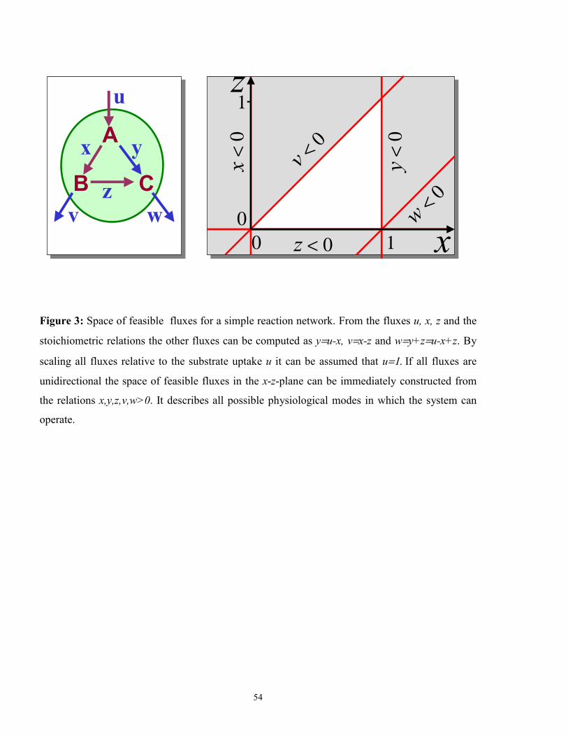
54

A

CB

u

wv

x y

z

x

z

x=<=

0

v=<=

0

y=<=

0

z=<=0w=<

=

0

00

1

1

Figure 3: Space of feasible fluxes for a simple reaction network. From the fluxes u, x, z and the

stoichiometric relations the other fluxes can be computed as y=u-x, v=x-z and w=y+z=u-x+z. By

scaling all fluxes relative to the substrate uptake u it can be assumed that u=1.=If all fluxes are

unidirectional the space of feasible fluxes in the x-z-plane can be immediately constructed from

the relations x,y,z,v,w>0. It describes all possible physiological modes in which the system can

operate.

55

z

x

u

A

CBwv

x y

z

Mode 1

A

CB

u

wv

x y

zMode 2

A

CB

u

wv

x y

zMode 3

feasiblefluxes

Figure 4: Extremal points of the feasible flux space from Figure 3. To each extremal point corre-

sponds a certain physiological mode of the network where several fluxes vanish. The nonvanish-

ing fluxes constitute a biochemical pathway that can operate autonomously. Alternatively the

extremal points can be interpreted as physiological operation modes that minimize or maximize

certain fluxes in the network.

56

1 2 3 4

1 2 3 4Carbon Atom Flux

u

E

D

B

A

B Cforward

backward

Bidirectional Reactions

v

Isotopomers

B

12C

13C

Figure 5: New concepts that distinguish the 13C metabolic flux analysis method from pure stoi-

chiometric flux analysis: i) The carbon atom transitions of each reaction step must be known. In

the example the second carbon atom of D becomes the first carbon atom of B in the reaction

step u. ii) The forward and backward reaction of a bidirectional reaction step can be distin-

guished. iii) Balance equations must be formulated for each isotopomer of all metabolites in the

system. The picture shows the 8 isotopomers of the metabolite B which has a carbon skeleton

with three carbon atoms.

57

Metabolic Network

X

E

0d

:0:

=⋅

−−

=⋅−−µτµτσ

mEcT

Generalized Reactionsσ=:=S ====T

µ:=c=T + d=E ===X

τ=:=T=====Em:=E=

Stoichiometry

µ

m

τTS σ

Kinetics

0

max

)()()(

mSmKSSS m

=+⋅= σσ

Figure 6: Derivation of Pirt’s classical maintenance model for cellular growth from a generalized

reaction network with abstract lumped pools and formal reaction kinetics. Pools: S-substrate, T-

intracellular intermediate, E-energy, X-biomass. Fluxes: σ-substrate uptake, µ-growth rate, τ-

energy production, m-maintenance. The (abstract) pool units are chosen such that only two gen-

eralized stoichiometric coefficients c,d are required. From the stoichiometric relations the growth

rate and energy production can be represented as στσµ ⋅+⋅=⋅+−=⋅+ dmcdcmdc )(,)( .

Filling in formal kinetic terms for σ and m completes the classical maintenance model.

58

Time

SubstrateC

onc.

MeOH-40 C

o

Figure 7: Schematic representation of a rapid sampling experiment. The microorganism is culti-

vated in a continuously driven bioreactor. A substrate pulse is imposed to stimulate an intracel-

lular metabolic response. Samples are taken in very short time intervals (5 Hz) and the cell me-

tabolism is stopped by methanol quenching. Afterwards the cells are disrupted and the intracel-

lular pool sizes are measured (Schaefer, 1999).

59

IntracellularConcentrations

EnzymeControl

MetabolicRegulationMetabolicRegulation

rapidsimpleinflexible

Time Scale10-5 - 102 sec

MetabolismMetabolism

GeneticRegulationGenetic

Regulation

slow expensiveadaptive

EnzymeSynthesis

Time Scale103 - 108 sec

Figure 8: Cascaded structure of the metabolic and genetic regulation networks. While metabolic

regulation on the enzyme level takes place at the short time scale, genetic regulation has much

larger time constants but is adaptive with respect to changing external conditions.

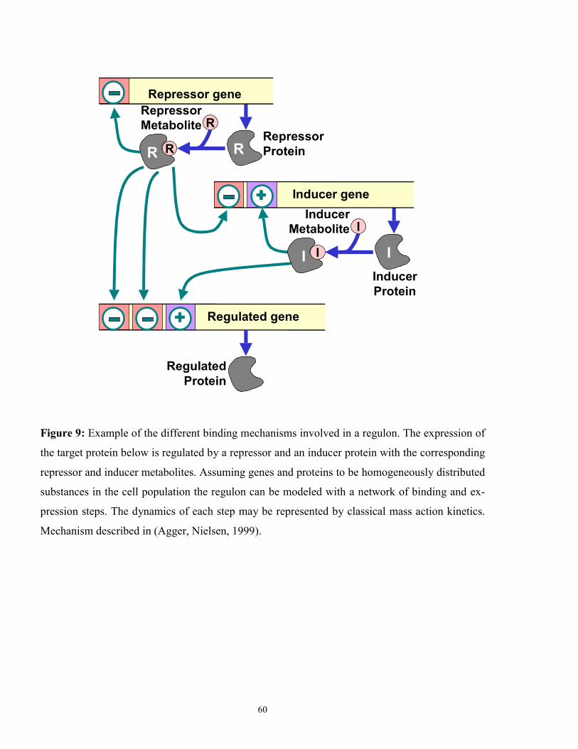
60

R

RRepressorMetabolite

I

I

Repressor gene

++++ Inducer gene

++++ Regulated gene

RepressorProtein

InducerProtein

InducerMetabolite

RegulatedProtein

RR

II

Figure 9: Example of the different binding mechanisms involved in a regulon. The expression of

the target protein below is regulated by a repressor and an inducer protein with the corresponding

repressor and inducer metabolites. Assuming genes and proteins to be homogeneously distributed

substances in the cell population the regulon can be modeled with a network of binding and ex-

pression steps. The dynamics of each step may be represented by classical mass action kinetics.

Mechanism described in (Agger, Nielsen, 1999).