modeling bond return predictability - nbb.be bond return predictability antonio gargano1 davide...

Modeling Bond Return Predictability

Antonio Gargano1 Davide Pettenuzzo2 Allan Timmermann3

1University of Melbourne 2Brandeis University

3UC San Diego

Gargano, Pettenuzzo, Timmermann Bond Return Predictability 03/2014 1/55

Predictability of bond returns

Literature on predictability of bond excess returns

Fama and Bliss (1987, AER): Forward spreadCampbell and Shiller (1991, JF): Treasury yield spreadsCochrane and Piazzesi (2005, AER): Linear combination of five forwardspreadsLudvigson and Ng (2008, RFS): Macro factors

Literature uses simple linear regression methods


Predictability of bond returns: Existing research

Literature reports large and highly significant R2-values usingoverlapping one-year returns

18% (Fama and Bliss)30-35% (Cochrane-Piazzesi)Wei and Wright (JAE, 2011): finite sample issues with highlypersistent, lagged endogenous regressors—reverse regressions

In-sample versus out-of-sample (OoS) results

Ludvigsson and Ng (RFS, 2008): some OoS predictability

Economic versus statistical measures of forecast performance

Thornton and Valente (2012), Sarno et al. (2014): OoS predictabilitycannot be exploited for economic gains

Macro-finance approaches

Dewachter, Iania, Lyrio (2014): weak OoS predictability


Modeling approach in this paper

Develop Bayesian modeling approach

Generate density forecasts—important for utility and log-score evaluation

Account for parameter estimation error

Thornton and Valente (RFS, 2012) use shrinkage for mean parameters

Incorporate stochastic volatility and time-varying parameters

Thornton and Valente (2012) use rolling-window estimate of volatility

Account for model uncertainty

Geweke-Amisano (JoE 2011) optimal pool (log-score criterion)


Empirical contributions

Most studies use a one-year return horizon, overlapping data

Here: new data with non-overlapping monthly excess bond returns

Time-varying parameters and stochastic volatility—e.g., 1979-1982

Term structure of return predictability: Study bond returnpredictability at monthly, quarterly, annual horizons

Reconcile evidence on statistical and economic measures of returnpredictability

Our empirical findings uncover both economic and statistical gains


1 Introduction

2 Data construction

3 Regression Models

4 Estimation MethodsLinear modelStochastic Volatility modelTime-varying Parameter ModelTime-varying Parameter, Stochastic Volatility Model

5 Empirical Results

6 Forecast Combinations


Data construction

Gurkaynak et al. (2007) reconstruct the entire yield curve for n-periodbonds using Nelson-Siegel smoothing methods:

y (n)t = β0 + β1

1− exp(− n

τ1

)nτ1

+ β2

1− exp(− n

τ1

)nτ1

− exp(− n

τ1

)+β3

1− exp(− n

τ2

)nτ2

− exp(− n

τ2

)Gurkaynak et al. estimate the parameters (β0, β1, β2, β3, τ1, τ2) ondaily cross-sections

We use log yields ranging from 12 months to 60 months and focus onthe last day of each month’s estimated log yields


Constructing excess returns and forward rates

h : frequency at which returns are computed: h = 1, 3, 12 formonthly, quarterly and annual data

n : maturity (in years) of bonds

For any n and h returns and forward rates are computed as follows:

1 Returns and excess returns (for n > h/12):

r (n)t+h/12 =p(n−h/12)t+h/12 − p

(n)t = ny (n)t − (n− h/12)y (n−h/12)

t+h/12

rx (n)t+h/12 =r(n)t+h/12 − y

h/12t (h/12)

2 Forward rates:

f (n−h/12,n)t = p(n−h/12)

t − p(n)t = ny (n)t − (n− h/12)y (n−h/12)t


In-sample regressions

Regressions use non-overlapping bond returns on data from 1962:01to 2011:12

We consider all possible model combinations obtained from threecommon predictors from the literature

Forward spreads (Fama-Bliss)Linear combination of forward rates (Cochrane-Piazzesi)Linear combination of macro factors (Ludvigson-Ng)

Forward spreads (Fama-Bliss)

fs(n,h)t = f (n−h/12,n)t − y (h/12)

t (h/12)


Cochrane-Piazzesi (2005) factor

m : set containing the predicted maturities. The Cochrane-Piazzesifactor is

f(n−h/12,n|m)t = γ′CP f

(n−h/12,n)t

for n = [1, 2, 3, 4, 5] and m = [2, 3, 4, 5], γCP is obtained from

1dim(m) ∑

mrx (m)t+h/12 =γ0 + γ′CP f

(n−h/12,n)t + εt+h/12

=γ0 + γ1f(n1−h/12,n1)t + γ2f

(n2−h/12,n2)t

+ ...+ γk f(nk−h/12,nk )t + εt+h/12

f(n−h/12,n)t =

[f (n1−h/12,n1)t , f (n2−h/12,n2)

t , ..., f (nk−h/12,nk )t

]Gargano, Pettenuzzo, Timmermann Bond Return Predictability 03/2014 10/55

Ludvigson-Ng Macro factor

T ×M panel of macroeconomic data xi ,t with factor structure

xi ,t = λi ,tgt + εi ,t

gt : estimate of r × 1 vector gt obtained through PC analysisFollowing Ludvigson & Ng, we use G5t = [g1,t , g31,t , g3,t , g4,t , g8,t ] tobuild a single linear combination of these factors:

G5(m)t = γ′LNG5t ,

γ is obtained from a regression

1dim(m) ∑

mrx (m)t+N/12 =γ0 + γ′LNG5t + ut+1

=γ0 + γ1g1,t + γ2g31,t + γ3g3,t

+ γ4g4,t + γ5g8,t + ut+1


Monthly Regression Models

Time and increments of time are measured in months

Sample period: 1962:1 to 2012:12

We predict one month ahead each month

Expectation Hypothesis (no predictability) benchmark

rx (n)t+1 = β0 + εt+1


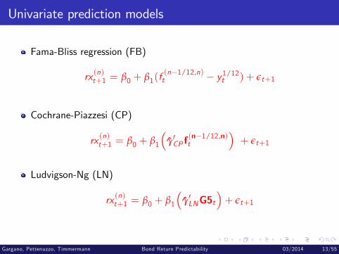
Univariate prediction models

Fama-Bliss regression (FB)

rx (n)t+1 = β0 + β1(f(n−1/12,n)t − y1/12

t ) + εt+1

Cochrane-Piazzesi (CP)

rx (n)t+1 = β0 + β1

(γ′CP f

(n−1/12,n)t

)+ εt+1

Ludvigson-Ng (LN)

rx (n)t+1 = β0 + β1

(γ′LNG5t

)+ εt+1


Bi- and trivariate prediction models

Fama-Bliss, Cochrane Piazzesi (FB-CP)

rx (n)t+1 = β0 + β1(f(n−1/12,n)t − y1/12

t ) + β2γ′CP f

(n−1/12,n)t + εt+1

Fama-Bliss, Ludvigson-Ng (FB-LN)

rx (n)t+1 = β0 + β1(f(n−1/12,n)t − y1/12

t ) + β2γ′LNG5t + εt+1

Cochrane-Piazzesi, Ludvigson-Ng (CP-LN)

rx (n)t+1 = β0 + β1γ′CP f

(n−1/12,n)t + β2γ

′LNG5t + εt+1

Fama-Bliss, Cochrane-Piazzesi, Ludvigson-Ng (FB-CP-LN)

rx (n)t+1 = β0 + β1(f(n−1/12,n)t − y1/12

t ) + β2γ′CP f

(n−1/12,n)t

+β3γ′LNG5t + εt+1


Linear regression model

Model bond excess returns rx (n)τ+1 as a linear function of lagged

predictor variables, x(n)τ

rx (n)τ+1 = µ+ β′x(n)τ + ετ+1, τ = 1, ..., t − 1,ετ+1 ∼ N(0, σ2ε )

Priors for µ and β are assumed to be normal and independent of σ2ε[µβ

]∼ N (b,V )

We use a "no-predictability" prior

b =

[rx (n)t0

], V = ψ2

[s2rx ,t

t−1∑τ=1

x(n)τ x(n)′τ

].


Priors (linear model)

Data-based moments

rx (n)t =1

t − 1t−1∑τ=1

rx (n)τ+1,

s2rx ,t =1

t − 2t−1∑τ=1

(rx (n)τ+1 − rx

(n)t

)2ψ = n/2 : controls the tightness of the prior: ψ→ ∞ yields diffusepriors on µ and β

Gamma prior for the error precision of the return innovation, σ−2ε :

σ−2ε ∼ G(s−2rx ,t , v0 (t − 1)

)v0 = 2/n : prior hyperparameter that controls the informativeness.v0 → 0 yields a diffuse prior on σ−2ε


Draws from linear Model

Draws from the joint posterior distribution p(

µ, β, σ−2ε

∣∣Dt) combinepriors with the likelihood function to get posteriors:[

µβ

]∣∣∣∣ σ−2ε ,Dt ∼ N(b,V

),

σ−2ε

∣∣ µ, β,Dt ∼ G(s−2, v

)Gibbs sampler can be used to iterate back and forth between blocksof parameters

(µ, β, σ−2ε

)Draws from the predictive density p

(rx (n)t+1

∣∣∣Dt) are obtained fromp(rx (n)t+1

∣∣∣Dt) =∫

µ,β,σ−2ε

p(rx (n)t+1

∣∣∣ µ, β, σ−2ε ,Dt)p(

µ, β, σ−2ε

∣∣Dt)×dµdβdσ−2ε


Stochastic Volatility (SV) model

SV model:

rx (n)τ+1 = µ+ β′x(n)τ + exp (hτ+1) uτ+1, uτ+1 ∼ N (0, 1)

hτ+1 : (log of) bond return volatility at time τ + 1

log-volatility is assumed to evolve as a driftless random walk

hτ+1 = hτ + ξτ+1, ξτ+1 ∼ N(0, σ2ξ

)


Priors for SV Model

Writing p(ht , σ−2ξ

)= p

(ht | σ−2ξ

)p(

σ−2ξ

), we have

p(ht∣∣ σ−2ξ

)=

t−1∏τ=1

p(hτ+1| hτ, σ

−2ξ

)p (h1)

hτ+1| hτ, σ−2ξ ∼ N

(hτ, σ

2ξ

)To complete the prior elicitation for p

(ht , σ−2ξ

)we only need to

specify priors for h1, the initial log volatility, and σ−2ξ :

h1 ∼ N (ln (srx ,t ) , kh)

σ−2ξ ∼ G(1/kξ , 1

)Choose hyperparameters to imply uninformative priors, allowing thedata to determine the degree of time variation in return volatility


Draws from Stochastic Volatility Model

To obtain draws from the joint posterior distributionp(

µ, β, ht , σ−2ξ

∣∣∣Dt) under the SV model, we use the Gibbs samplerto draw recursively from the following three conditional distributions:

1 p(ht | µ, β, σ−2ξ ,Dt

).

2 p(

µ, β| ht , σ−2ξ ,Dt).

3 p(

σ−2ξ

∣∣∣ µ, β, ht ,Dt).

We employ the algorithm of Kim et al. (1998) to simulate from theseblocks


Draws from SV model (cont.)

Draws from the predictive density p(rx (n)t+1

∣∣∣Dt) :

p(rx (n)τ+1

∣∣∣Dt) =∫

µ,β,ht+1,σ−2ξ

p(rx (n)τ+1

∣∣∣ ht+1, µ, β, ht , σ−2ξ ,Dt)

×p(ht+1| µ, β, ht , σ−2ξ ,Dt

)×p(


∣∣∣Dt) dµdβdht+1dσ−2ξ .

p(rx (n)t+1

∣∣∣ ht+1, µ, β, ht , σ−2ξ ,Dt): predictive density of excess returns

given the model parameters

p(ht+1| µ, β, ht , σ−2ξ ,Dt

): reflects how period t + 1 volatility may

drift away from ht over time

p(


∣∣∣Dt) : parameter uncertainty in the sample


Draws from SV model (cont.)

To obtain draws from p(rx (n)t+1

∣∣∣Dt), we proceed in three steps:1 Simulate from p

(µ, β, ht , σ−2ξ

∣∣∣Dt): draws fromp(


∣∣∣Dt) are obtained from the Gibbs sampling algorithm2 Simulate from p

(ht+1| µ, β, ht , σ−2ξ ,Dt

): For a given ht and σ−2ξ , µ

and β and prior volatilities up to t become redundant, i.e.,

p(ht+1| µ, β, ht , σ−2ξ ,Dt

)= p

(ht+1| ht , σ−2ξ ,Dt

), so

ht+1| ht , σ−2ξ ,Dt ∼ N(ht , σ2ξ

)3 Simulate from p

(rx (n)t+1

∣∣∣ ht+1, µ, β, ht , σ−2ξ ,Dt): For a given ht+1, µ,

and β, use that

rx (n)t+1

∣∣∣ ht+1, µ, β,Dt ∼ N (µ+ β′x(n)τ , exp (ht+1))


Time-varying parameter (TVP) model

rx (n)τ+1 = µτ + β′τx(n)τ + ετ+1, τ = 1, ..., t − 1,

ετ+1 ∼ N(0, σ2ε ).

Assume that θτ =(µτ, β

′τ

)′follows a random walk:

θτ+1 = θτ + ητ+1, ητ+1 ∼ N (0,Q) .

We work with an equivalent version which sets θ1 = 0 and uses

rx (n)τ+1 = (µ+ µτ) + (β+ βτ)′ x(n)τ + ετ+1, τ = 1, ..., t − 1,

ετ+1 ∼ N(0, σ2ε ).


TVP model: Choice of priors

For [µ, β]′ and σ2ε , we follow the same prior choices made under thelinear model section:[

µβ

]∼ N (b,V ) ,

σ−2ε ∼ G(s−2rx ,t , v0 (t − 1)

)


TVP model: Choice of priors (cont.)

TVP model also elicits a joint prior for the sequence θt = {θ2, ..., θt}and the covariance matrix QFor θt and Q, we first write p (θt ,Q) = p

(θt∣∣Q) p (Q), and note

that

p(

θt∣∣Q) = t−1

∏τ=1

p (θτ+1| θτ,Q) , θτ+1| θτ,Q ∼ N (θτ,Q) .

To complete the prior elicitation for p (θt ,Q) , we only need tospecify priors for Q:

Q ∼ IW (Q, t − 2)

Q = kQ (t − 2)

s2rx ,t(t−1∑τ=1

x(n)τ x(n)′τ

)−1 .kQ controls the time-variation in the coeffi cients θτ


Time-varying parameter, SV model

Consider a model with both TVP and SV:

rx (n)τ+1 = µτ + β′τx(n)τ + exp (hτ+1) uτ+1,

θτ+1 = θτ + ητ+1,

hτ+1 = hτ + ξτ+1, ητ+1 ∼ N (0,Q) ,

ξτ+1 ∼ N(0, σ2ξ

)

Once again, we set θ1 = 0 and use

rx (n)τ+1 = (µ+ µt ) + (β+ βτ)′ x(n)τ + exp (hτ+1) uτ+1


TVP-SV model: Priors

Our choice of priors combines those made for the TVP and SVmodels: [

µβ

]∼ N (b,V )

σ−2ε ∼ G(s−2rx ,t , v0 (t − 1)

)along with

h1 ∼ N (ln (srx ,t ) , kh)

σ−2ξ ∼ G(1/kξ , 1

)Q ∼ IW (Q, t − 2)


Empirical Results: 2-5 year bond excess returns

Exc

ess

retu

rns

(%)

n = 2 years

1960 1965 1970 1975 1980 1985 1990 1995 2000 2005 2010−10

−8

−6

−4

−2

0

2

4

6

8

10

Exc

ess

retu

rns

(%)

n = 3 years

1960 1965 1970 1975 1980 1985 1990 1995 2000 2005 2010−10

−8

−6

−4

−2

0

2

4

6

8

10

Exc

ess

retu

rns

(%)

n = 4 years

1960 1965 1970 1975 1980 1985 1990 1995 2000 2005 2010−10

−8

−6

−4

−2

0

2

4

6

8

10

Exc

ess

retu

rns

(%)

n = 5 years

1960 1965 1970 1975 1980 1985 1990 1995 2000 2005 2010−10

−8

−6

−4

−2

0

2

4

6

8

10


Descriptive statistics

Bonds Stocks2 years 3 years 4 years 5 years S&P

Panel A: Monthlymean 1.4147 1.7316 1.9868 2.1941 3.7327st.dev. 2.9711 4.1555 5.2174 6.2252 15.2939skew 0.4995 0.2079 0.0566 0.0149 -0.6314kurt 14.8625 10.6482 7.9003 6.5797 5.3510AC(1) 0.1692 0.1533 0.1384 0.1235 0.0601AC(2) -0.0624 -0.0655 -0.0651 -0.0660 -0.0360AC(3) -0.0437 -0.0383 -0.0282 -0.0197 0.0362Sharpe 0.4761 0.4167 0.3808 0.3525 0.2441


OLS regression estimates

Panel A: Monthly(1) (2) (3) (4) (5) (6) (7)

2 yearsFB 1.1648*** 0.6621** 1.3592*** 1.1221***CP 0.6548*** 0.5123*** 0.4905*** 0.2317LN 0.6712*** 0.7091*** 0.6099*** 0.6736***adjR2 0.0166 0.0246 0.0580 0.0277 0.0812 0.0708 0.0821



5 yearsFB 1.9726*** 1.2280** 1.9093*** 1.4876***CP 1.3612*** 0.9640*** 1.0441*** 0.5502*LN 1.3070*** 1.2888*** 1.1765*** 1.2240***adjR2 0.0211 0.0242 0.0499 0.0292 0.0697 0.0630 0.0712


Parameters for FB+CP+LN model

β1

1960 1965 1970 1975 1980 1985 1990 1995 2000 2005 20100

0.5

1

1.5LinearTVPSVTVP−SV

β2

1960 1965 1970 1975 1980 1985 1990 1995 2000 2005 20100

0.2

0.4

0.6

0.8

β3

1960 1965 1970 1975 1980 1985 1990 1995 2000 2005 20100

0.5

1

σ

1960 1965 1970 1975 1980 1985 1990 1995 2000 2005 20100

2

4

6


Posterior parameter distributions

−0.8 −0.6 −0.4 −0.2 0 0.2 0.4 0.60

1

2

3

4

5

6

7

8

9

β0

LinearTVPSVTVP−SV

−3 −2 −1 0 1 2 3 40

0.2

0.4

0.6

0.8

1

1.2

1.4

β1

−2 −1.5 −1 −0.5 0 0.5 1 1.5 2 2.50

0.5

1

1.5

2

2.5

β2

−0.4 −0.2 0 0.2 0.4 0.6 0.8 1 1.2 1.4 1.60

0.5

1

1.5

2

2.5

3

3.5

4

4.5

β3


Out-of-sample analysis

Predict 2, 3, 4, and 5 year bond returns (i.e. n = 2, 3, 4, 5)

Expanding estimation window

CP and LN factors are constructed recursively

Out-of-sample-period: 1990 - 2011

Predictability is studied separately for each maturity


Out-of-sample analysis (cont.)

Following Goyal and Welch (2008) we report recursively computeddifferences in the cumulative sum of squared errors (SSE) between theEH model and the ith model:

∆CumSSE (n)t =t

∑τ=t

(e(n)τ

)2−

t

∑τ=t

(e(n)τ,i

)2.

Similarly, following Campbell and Thompson (2008), we compute theout-of-sample R2 of model i relative to the EH model as

R (n)2OoS ,i = 1−∑t

τ=t e(n)2τ,i

∑tτ=t e

(n)2τ

.


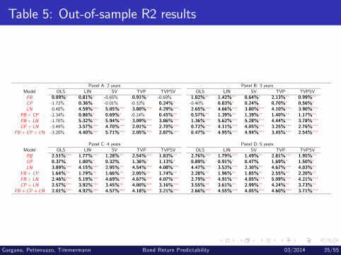
Table 5: Out-of-sample R2 results

Panel A: 2 years Panel B: 3 yearsModel OLS LIN SV TVP TVPSV OLS LIN SV TVP TVPSVFB 0.09%∗ 0.81%∗ -0.65% 0.91%∗ -0.60% 1.82%∗∗ 1.42%∗∗ 0.64%∗ 2.13%∗∗ 0.99%∗∗

CP -1.72% 0.36% -0.01% -0.32% 0.24%∗ -0.40% 0.83%∗ 0.24% 0.70%∗ 0.56%∗

LN -0.40% 4.59%∗∗∗ 5.05%∗∗∗ 3.80%∗∗∗ 4.29%∗∗∗ 2.65%∗∗∗ 4.66%∗∗∗ 3.80%∗∗∗ 4.10%∗∗∗ 3.90%∗∗∗

FB + CP -1.34% 0.86%∗ 0.69%∗ -0.14% 0.45%∗∗ 0.57%∗∗ 1.39%∗∗ 1.39%∗∗ 1.40%∗∗ 1.17%∗∗

FB + LN -1.70% 5.32%∗∗∗ 5.94%∗∗∗ 3.09%∗∗∗ 3.86%∗∗∗ 1.36%∗∗∗ 5.62%∗∗∗ 5.28%∗∗∗ 4.44%∗∗∗ 3.78%∗∗∗

CP + LN -3.49% 3.57%∗∗∗ 4.70%∗∗∗ 2.01%∗∗∗ 2.70%∗∗∗ 0.72%∗∗∗ 4.11%∗∗∗ 4.05%∗∗∗ 3.25%∗∗∗ 2.76%∗∗∗

FB + CP + LN -3.20% 4.40%∗∗∗ 5.71%∗∗∗ 2.05%∗∗∗ 2.87%∗∗∗ 0.47%∗∗∗ 4.95%∗∗∗ 4.94%∗∗∗ 3.45%∗∗∗ 2.54%∗∗∗

Panel C: 4 years Panel D: 5 yearsModel OLS LIN SV TVP TVPSV OLS LIN SV TVP TVPSVFB 2.51%∗∗∗ 1.77%∗∗∗ 1.28%∗∗ 2.54%∗∗∗ 1.83%∗∗ 2.76%∗∗∗ 1.79%∗∗∗ 1.49%∗∗ 2.81%∗∗∗ 1.95%∗∗

CP 0.37% 1.00%∗ 0.32% 1.36%∗ 1.13%∗ 0.89%∗ 0.91%∗ 0.47% 1.69%∗ 1.50%∗

LN 3.89%∗∗∗ 4.15%∗∗∗ 2.95%∗∗ 4.54%∗∗∗ 4.08%∗∗∗ 4.47%∗∗∗ 3.53%∗∗∗ 2.30%∗∗ 4.67%∗∗∗ 4.03%∗∗

FB + CP 1.64%∗∗ 1.79%∗∗ 1.66%∗∗ 2.05%∗∗ 1.74%∗∗ 2.28%∗∗ 1.96%∗∗ 1.85%∗∗ 2.55%∗∗ 2.20%∗∗

FB + LN 2.46%∗∗∗ 5.19%∗∗∗ 4.69%∗∗∗ 4.67%∗∗∗ 4.07%∗∗∗ 2.79%∗∗∗ 4.91%∗∗∗ 4.05%∗∗∗ 5.09%∗∗∗ 4.21%∗∗∗

CP + LN 2.57%∗∗∗ 3.92%∗∗∗ 3.45%∗∗ 4.00%∗∗∗ 3.16%∗∗∗ 3.55%∗∗ 3.61%∗∗ 2.99%∗∗ 4.24%∗∗ 3.73%∗∗

FB + CP + LN 2.01%∗∗∗ 4.92%∗∗∗ 4.57%∗∗∗ 4.18%∗∗∗ 3.21%∗∗∗ 2.66%∗∗∗ 4.55%∗∗∗ 4.05%∗∗∗ 4.60%∗∗∗ 3.71%∗∗∗


CumSum squared plots for six models, n = 5

∆ cu

mul

ativ

e S

SE

FB

1985 1990 1995 2000 2005 2010−10

0

10

20

30

40LinearTVPSVTVP−SV

∆ cu

mul

ativ

e S

SE

CP

1985 1990 1995 2000 2005 2010−10

0

10

20

30

40

∆ cu

mul

ativ

e S

SE

LN

1985 1990 1995 2000 2005 2010−10

0

10

20

30

40

∆ cu

mul

ativ

e S

SE

FB + LN

1985 1990 1995 2000 2005 2010−10

0

10

20

30

40

∆ cu

mul

ativ

e S

SE

CP + LN

1985 1990 1995 2000 2005 2010−10

0

10

20

30

40

∆ cu

mul

ativ

e S

SE

FB + CP + LN

1985 1990 1995 2000 2005 2010−10

0

10

20

30

40


Out-of-sample analysis (cont.)

To evaluate the accuracy of the density forecasts, we use the logpredictive score which is commonly viewed as the broadest measure ofdensity accuracy.Denote by LSt and LSti the log of the predictive densities evaluatedat the observed bond excess return r (n)tUse these as inputs to the period-t difference in the cumulative logscore differentials (LS) between the EH model and the ith model:

∆CumLSt =t

∑τ=t[LSτ.i − LSτ] .

Following Clark and Ravazzolo (JAE, 2014) we compute the averagelog predictive scores differential of model i relative to the EH model as

LS i =1

t − t + 1t

∑τ=t(LSτ.i − LSτ)

a positive LS i indicates that model i beats the EH benchmark.Gargano, Pettenuzzo, Timmermann Bond Return Predictability 03/2014 37/55

Statistical evaluation of results

Point forecasts use a DM test with finite-sample correction(Harvey-Leybourne-Newbold)

Log predictive score test uses DM test based on equality of averagelog scores

Clark and Ravazzolo (JAE, 2014)Clark and McCracken (JoE, 2011) show that for nested models the DMtest yield conservative finite-sample inference

t-test uses Andrews-Monahan (EcTa, 1992) pre-whitened quadraticspectral estimator


Table 6: Predictive Bayes factors

Panel A: 2 years Panel B: 3 yearsModel LIN SV TVP TVPSV LIN SV TVP TVPSVFB 0.002 0.248∗∗∗ -0.001 0.220∗∗∗ 0.003 0.121∗∗∗ 0.001 0.097∗∗∗

CP 0.004 0.239∗∗∗ -0.000 0.202∗∗∗ 0.005∗∗ 0.119∗∗∗ 0.002 0.095∗∗

LN 0.009∗ 0.252∗∗∗ 0.005 0.207∗∗∗ 0.012∗∗ 0.130∗∗∗ 0.005 0.087∗∗

FB + CP 0.004 0.243∗∗∗ -0.000 0.194∗∗∗ 0.005∗ 0.120∗∗∗ 0.002 0.083∗∗

FB + LN 0.014∗∗ 0.257∗∗∗ 0.007 0.204∗∗∗ 0.015∗∗ 0.131∗∗∗ 0.009 0.075∗∗

CP + LN 0.010∗ 0.240∗∗∗ 0.004 0.183∗∗∗ 0.012∗∗ 0.126∗∗∗ 0.007 0.073∗

FB + CP + LN 0.011∗∗ 0.250∗∗∗ 0.004 0.176∗∗∗ 0.014∗∗ 0.125∗∗∗ 0.006 0.047

Panel C: 4 years Panel D: 5 yearsModel LIN SV TVP TVPSV LIN SV TVP TVPSVFB 0.006∗∗ 0.067∗∗∗ 0.004 0.045∗ 0.006∗∗ 0.033∗ 0.006 0.016CP 0.006∗∗ 0.066∗∗∗ 0.005 0.046∗ 0.005∗∗ 0.028 0.007 0.015LN 0.013∗∗ 0.076∗∗∗ 0.011 0.041 0.012∗∗ 0.036∗ 0.013 0.013

FB + CP 0.008∗∗ 0.063∗∗ 0.006 0.034 0.008∗∗ 0.033∗ 0.009 0.004FB + LN 0.016∗∗ 0.075∗∗∗ 0.012 0.026 0.016∗∗ 0.040∗ 0.014 -0.002CP + LN 0.013∗∗ 0.072∗∗ 0.012 0.026 0.014∗∗ 0.037∗ 0.014 -0.004

FB + CP + LN 0.016∗∗ 0.072∗∗ 0.012 0.002 0.017∗∗ 0.033 0.014 -0.020


Economic value of return forecasts

Investor puts weight ωt on an n−period risky bond and (1−ωt ) on1-month T-bill that pays the riskfree rate, r ftInvestor has power utility and coeffi cient of relative risk aversion A:

U (ωt , rt+1) =

[(1−ωt ) exp

(r ft)+ωt exp

(r ft + rx

nt+1

)]1−A1− A

A = 10

Using information at time t, Dt , the investor solves the optimal assetallocation problem

ω∗t = argmaxωt

∫U (ωt , rxt+1) p

(rxt+1| Dt

)drxt+1


Economic value of return forecasts

Approximate expected utility integral by generating a large number ofdraws, rx jt+1,i , j = 1, .., J, from the predictive densities:

ωt ,i = maxωt

1J

J

∑j=1

[(1−ωt ) exp

(r ft)+ωt exp

(r ft + rx

jt+1,i

)]1−A1− A

To avoid bankruptcy concerns, we restrict the weights on the riskybonds to the interval [0, 0.99]

Sequence of portfolio weights{

ωEHt

}and {ωt ,i} are used to

compute realized utilities and converted into CER-values


Table 7: Out-of-sample CER values, A = 10

Panel A: 2 years Panel B: 3 yearsModel LIN SV TVP TVPSV LIN SV TVP TVPSVFB -0.23% -0.25% -0.21% -0.25% 0.05% 0.17% 0.18% 0.08%CP -0.19% 0.04% -0.24% 0.06% -0.08% 0.21% -0.16% 0.28%LN 0.11% 0.10% 0.09% 0.09% 0.57% 0.64% 0.66% 0.66%

FB + CP -0.21% -0.13% -0.27% -0.10% 0.01% 0.26% 0.08% 0.16%FB + LN 0.07% 0.12% -0.07% 0.01% 0.53% 0.67% 0.38% 0.42%CP + LN 0.09% 0.19% -0.04% 0.01% 0.49% 0.67% 0.46% 0.48%

FB + CP + LN 0.05% 0.14% -0.09% 0.02% 0.47% 0.62% 0.32% 0.43%

Panel C: 4 years Panel D: 5 yearsModel LIN SV TVP TVPSV LIN SV TVP TVPSVFB 0.46% 0.58% 0.56% 0.63% 0.69% 0.74% 0.84% 0.88%CP 0.12% 0.25% 0.15% 0.28% 0.23% 0.35% 0.31% 0.43%LN 0.90% 0.96% 1.19% 1.22% 0.90% 0.97% 1.37% 1.47%

FB + CP 0.38% 0.61% 0.46% 0.62% 0.62% 0.81% 0.71% 0.79%FB + LN 1.03% 1.17% 0.91% 0.83% 1.25% 1.33% 1.26% 1.19%CP + LN 0.73% 1.01% 0.97% 0.97% 0.79% 1.03% 1.13% 1.28%

FB + CP + LN 0.98% 1.13% 0.84% 0.90% 1.11% 1.21% 1.21% 1.19%


cumCER plot for A = 10, FB+CP+LN, n = 3

Con

tinuo

usly

com

poun

ded

CE

Rs

(%)

n=2 years

1985 1990 1995 2000 2005 2010−5

0

5

10

15

20

25

30

35

40LinearTVPSVTVP−SV

Con

tinuo

usly

com

poun

ded

CE

Rs

(%)

n=3 years

1985 1990 1995 2000 2005 2010−5

0

5

10

15

20

25

30

35

40

Con

tinuo

usly

com

poun

ded

CE

Rs

(%)

n=4 years

1985 1990 1995 2000 2005 2010−5

0

5

10

15

20

25

30

35

40

Con

tinuo

usly

com

poun

ded

CE

Rs

(%)

n=5 years

1985 1990 1995 2000 2005 2010−5

0

5

10

15

20

25

30

35

40


Predictability in expansions and recessions

LIN SV TVP TVPSVModel Exp Rec Exp Rec Exp Rec Exp Rec

Panel A: 2 yearsFB 2.86% 0.48% 3.05% 0.11% 4.53% 1.62% 5.49% -0.47%CP 1.53% 4.08%∗∗ 1.87% 3.24%∗ 3.68% 4.63%∗ 4.02% 3.53%∗

LN 1.23% 12.03%∗∗ 1.95% 7.87%∗∗∗ 2.05% 18.04%∗∗ 3.94% 11.54%∗∗

FB + CP 2.62% 3.72%∗ 3.08% 2.78% 5.94% 5.57%∗ 5.94% 2.39%FB + LN 4.97% 12.83%∗∗∗ 5.57% 8.39%∗∗ 6.40% 19.53%∗∗∗ 7.99% 13.42%∗∗

CP + LN 2.66% 13.47%∗∗ 3.41% 8.81%∗∗∗ 4.63% 19.67%∗∗ 5.68% 13.97%∗∗

FB + CP + LN 4.86% 13.51%∗∗∗ 5.56% 8.63%∗∗ 7.86% 20.82%∗∗∗ 8.35% 14.82%∗∗


Equal-weighted combinations

Equal-weighted pool (EWP), putting 1/N weight on each model Mi :

p(rx (n)t+1

∣∣∣Dt) = 1N

N

∑i=1p(rx (n)t+1

∣∣∣Mi ,Dt)

{p(rx (n)t+1

∣∣∣Mi ,Dt)}N

i=1: predictive densities

N = 21


Predictive pool combinations

Real time optimal predictive pool (RTOP) of Geweke and Amisano(2012):

p(rx (n)t+1

∣∣∣Dt) = N

∑i=1w ∗t ,i × p

(rx (n)t+1

∣∣∣Mi ,Dt)

We determine w∗t = [w ∗1t , ...,w∗Nt ] recursively by solving the following

maximization problem at time t,

w∗t = argmaxwt

t−1∑τ=1

log

[N

∑i=1wit × Sτ+1,i

]

w∗t restricted to the N−dimensional unit simplexSτ+1,i : time-τ + 1 recursively computed log score for model i , i.e.Sτ+1,i = exp (LSτ+1,i )

As t → ∞ these weights minimize the Kullback-Leibler distance


Bayesian Model Averaging

BMA weights:

p(rx (n)t+1

∣∣∣Dt) = N

∑i=1Pr(Mi | Dt

)p(rx (n)t+1

∣∣∣Mi ,Dt)

Pr (Mi | Dt ) : posterior probability of model i at time t:

Pr(Mi | Dt

)=

Pr({rx (n)τ+1}t−1τ=1

∣∣∣Mi

)Pr (Mi )

∑Nj=1 Pr

({rx (n)τ+1}t−1τ=1

∣∣∣Mj

)Pr (Mj )


∣∣∣Mi

): marginal likelihood for model i

Pr (Mi ) = 1/N : prior probability for model iWe compute the marginal likelihoods by cumulating the predictive logscores of each model over time:


∣∣∣Mi

)= exp

(t

∑τ=t

LSτ.i

).


Optimal prediction pool weightsO

ptim

al p

redi

ctio

n po

ol w

eigh

ts

n=2 years

1985 1990 1995 2000 2005 20100

0.1

0.2

0.3

0.4

0.5

0.6

0.7

0.8

0.9

1LINSVTVP

Opt

imal

pre

dict

ion

pool

wei

ghts

n=3 years

1985 1990 1995 2000 2005 20100

0.1

0.2

0.3

0.4

0.5

0.6

0.7

0.8

0.9

1

Opt

imal

pre

dict

ion

pool

wei

ghts

n=4 years

1985 1990 1995 2000 2005 20100

0.1

0.2

0.3

0.4

0.5

0.6

0.7

0.8

0.9

1

Opt

imal

pre

dict

ion

pool

wei

ghts

n=5 years

1985 1990 1995 2000 2005 20100

0.1

0.2

0.3

0.4

0.5

0.6

0.7

0.8

0.9

1


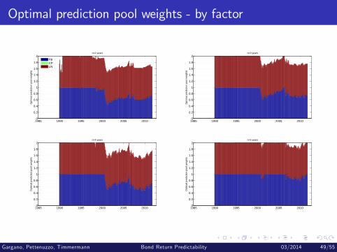
Optimal prediction pool weights - by factorO

ptim

al p

redi

ctio

n po

ol w

eigh

ts

n=2 years

1985 1990 1995 2000 2005 20100

0.2

0.4

0.6

0.8

1

1.2

1.4

1.6

1.8

2FBCPLN

Opt

imal

pre

dict

ion

pool

wei

ghts

n=3 years

1985 1990 1995 2000 2005 20100

0.2

0.4

0.6

0.8

1

1.2

1.4

1.6

1.8

2

Opt

imal

pre

dict

ion

pool

wei

ghts

n=4 years

1985 1990 1995 2000 2005 20100

0.2

0.4

0.6

0.8

1

1.2

1.4

1.6

1.8

2

Opt

imal

pre

dict

ion

pool

wei

ghts

n=5 years

1985 1990 1995 2000 2005 20100

0.2

0.4

0.6

0.8

1

1.2

1.4

1.6

1.8

2


cumSEE plot for model combinations

∆ cu

mul

ativ

e S

SE

n = 2 years

1985 1990 1995 2000 2005 2010−1

0

1

2

3

4

5

6Equal−weighted combinationOptimal prediction pool

∆ cu

mul

ativ

e S

SE

n = 5 years

1985 1990 1995 2000 2005 2010−5

0

5

10

15

20

25

30

35


cumCER plot for A = 10, model combinations

Con

tinuo

usly

com

poun

ded

CE

Rs

(%)

n=2 years

1985 1990 1995 2000 2005 2010−5

0

5

10

15

20

25

30

35

40Equal−weighted combinationOptimal prediction pool

Con

tinuo

usly

com

poun

ded

CE

Rs

(%)

n=3 years

1985 1990 1995 2000 2005 2010−5

0

5

10

15

20

25

30

35

40

Con

tinuo

usly

com

poun

ded

CE

Rs

(%)

n=4 years

1985 1990 1995 2000 2005 2010−5

0

5

10

15

20

25

30

35

40

Con

tinuo

usly

com

poun

ded

CE

Rs

(%)

n=5 years

1985 1990 1995 2000 2005 2010−5

0

5

10

15

20

25

30

35

40


Forecast Combinations

Method 2 years 3 years 4 years 5 yearsOut-of-sample R2

OW 5.92%∗∗∗ 5.55%∗∗∗ 5.05%∗∗∗ 5.16%∗∗∗

EW 4.99%∗∗∗ 4.39%∗∗∗ 4.16%∗∗∗ 3.85%∗∗∗

BMA 5.42%∗∗∗ 4.36%∗∗∗ 3.43%∗∗∗ 3.17%∗∗∗

Predictive LikelihoodOW 0.25∗∗∗ 0.11∗∗∗ 0.05∗∗∗ 0.03∗∗∗

EW 0.14∗∗∗ 0.08∗∗∗ 0.05∗∗∗ 0.04∗∗∗

BMA 0.25∗∗∗ 0.12∗∗∗ 0.05∗∗ 0.02CER

OW 0.15% 0.49% 0.98% 1.30%EW 0.10% 0.53% 0.96% 1.02%BMA 0.14% 0.63% 0.92% 1.14%


Table 8: Robustness to prior

Prior ψ = 5, ν = 0.2Panel A: 2 years Panel B: 3 years

Model OLS LIN SV OLS LIN SVFB 0.11%∗ 0.25%∗ -1.21% 1.77%∗∗ 1.76%∗∗ 0.90%∗∗

CP -1.69% -1.36% 0.14%∗ -0.45% -0.11% 0.66%∗

LN -0.38% 0.30%∗∗∗ 5.03%∗∗∗ 2.60%∗∗∗ 3.45%∗∗∗ 4.39%∗∗∗

FB + CP -1.31% -1.26% 0.34%∗∗ 0.53%∗∗ 0.86%∗∗ 1.90%∗∗

FB + LN -1.67% -0.91% 5.07%∗∗∗ 1.31%∗∗∗ 2.79%∗∗∗ 5.32%∗∗∗

CP + LN -3.46% -2.70% 4.42%∗∗∗ 0.68%∗∗∗ 1.74%∗∗∗ 4.53%∗∗∗

FB + CP + LN -3.17% -2.45% 4.83%∗∗∗ 0.43%∗∗∗ 1.88%∗∗∗ 5.06%∗∗∗

Panel C: 4 years Panel D: 5 yearsModel OLS LIN SV OLS LIN SVFB 2.39%∗∗ 2.47%∗∗∗ 1.72%∗∗ 2.65%∗∗∗ 2.57%∗∗∗ 2.18%∗∗

CP 0.25% 0.72% 0.92%∗ 0.77% 1.02%∗ 0.94%LN 3.77%∗∗∗ 4.58%∗∗∗ 3.79%∗∗∗ 4.35%∗∗∗ 4.76%∗∗∗ 3.00%∗∗

FB + CP 1.52%∗∗ 1.90%∗∗ 2.55%∗∗ 2.17%∗∗ 2.44%∗∗ 2.78%∗∗

FB + LN 2.34%∗∗∗ 4.60%∗∗∗ 5.27%∗∗∗ 2.67%∗∗∗ 5.41%∗∗∗ 4.96%∗∗∗

CP + LN 2.45%∗∗∗ 3.73%∗∗∗ 4.54%∗∗∗ 3.43%∗∗ 4.57%∗∗ 4.02%∗∗

FB + CP + LN 1.89%∗∗∗ 4.19%∗∗∗ 5.10%∗∗∗ 2.55%∗∗∗ 5.19%∗∗∗ 5.01%∗∗∗


Robustness to priors

Prior ψ = 5, ν = 0.2Panel A: 2 years Panel B: 3 years

Model OLS LIN SV OLS LIN SVFB 0.11%∗ 0.25%∗ -1.21% 1.77%∗∗ 1.76%∗∗ 0.90%∗∗

CP -1.69% -1.36% 0.14%∗ -0.45% -0.11% 0.66%∗

LN -0.38% 0.30%∗∗∗ 5.03%∗∗∗ 2.60%∗∗∗ 3.45%∗∗∗ 4.39%∗∗∗

FB + CP -1.31% -1.26% 0.34%∗∗ 0.53%∗∗ 0.86%∗∗ 1.90%∗∗

FB + LN -1.67% -0.91% 5.07%∗∗∗ 1.31%∗∗∗ 2.79%∗∗∗ 5.32%∗∗∗

CP + LN -3.46% -2.70% 4.42%∗∗∗ 0.68%∗∗∗ 1.74%∗∗∗ 4.53%∗∗∗

FB + CP + LN -3.17% -2.45% 4.83%∗∗∗ 0.43%∗∗∗ 1.88%∗∗∗ 5.06%∗∗∗

Panel C: 4 years Panel D: 5 yearsModel OLS LIN SV OLS LIN SVFB 2.39%∗∗ 2.47%∗∗∗ 1.72%∗∗ 2.65%∗∗∗ 2.57%∗∗∗ 2.18%∗∗

CP 0.25% 0.72% 0.92%∗ 0.77% 1.02%∗ 0.94%LN 3.77%∗∗∗ 4.58%∗∗∗ 3.79%∗∗∗ 4.35%∗∗∗ 4.76%∗∗∗ 3.00%∗∗

FB + CP 1.52%∗∗ 1.90%∗∗ 2.55%∗∗ 2.17%∗∗ 2.44%∗∗ 2.78%∗∗

FB + LN 2.34%∗∗∗ 4.60%∗∗∗ 5.27%∗∗∗ 2.67%∗∗∗ 5.41%∗∗∗ 4.96%∗∗∗

CP + LN 2.45%∗∗∗ 3.73%∗∗∗ 4.54%∗∗∗ 3.43%∗∗ 4.57%∗∗ 4.02%∗∗

FB + CP + LN 1.89%∗∗∗ 4.19%∗∗∗ 5.10%∗∗∗ 2.55%∗∗∗ 5.19%∗∗∗ 5.01%∗∗∗


Conclusion

Strong evidence of out-of-sample bond return predictability for 2-5year maturities

Ludvigson-Ng (2008) macro factor performs particularly well

Statistical return predictability carries over to economic returnpredictability

Accounting for SV improves economic and statistical performance

TVP model works well for the longer bond maturities

Forecast combination methods offer economic and statisticalimprovements


modeling bond return predictability - nbb.be bond return predictability antonio gargano1 davide...

Documents