Modeling Cavitation Erosion using Fluid-Material Interaction Simulations

Georges L. Chahine and Chao-Tsung Hsiao

DYNAFLOW, INC., 10621-J Iron Bridge Road, Jessup, MD, USA

ABSTRACT

Material deformation and pitting from cavitation bubble collapse is investigated

using fluid dynamics and material dynamics and their interaction. In the fluid, a novel

hybrid approach, which links a boundary element method and a compressible finite

difference method is used to capture nonspherical bubble dynamics and resulting liquid

pressures efficiently and accurately. The bubble dynamics is intimately coupled with a

finite element structure model to enable fluid/structure interaction simulations. Bubble

collapse loads the material with high impulsive pressures, which emanate from shock

waves, bubble reentrant jet impact on the material surface, and the collapse of the

remaining bubble ring. This produces high stress waves, which propagate into the

material and cause deformation. A pit (permanent deformation) is formed when the local

equivalent stresses exceed the material yield stress. The pressure loading depends on

bubble dynamics parameters such as the size of the bubble at its maximum volume, the

bubble standoff distance from the material wall, and the pressure driving the bubble

collapse. The effects of these parameters on the reentrant jet, the following bubble ring

collapse pressure, and the generated material pit characteristics are presented.

1 Introduction

Cavitation is the explosive growth and intense collapse of bubble nuclei in a liquid

when exposed to large pressure variations. It has been long known by the

hydrodynamics community for its deleterious effects in a variety of fluid machinery,

such as erosion, performance degradation, and noise and vibrations. A significant

amount of studies have been dedicated to seek out measures to mitigate if not eliminate

cavitation. Cavitation erosion attracts wide attention from materials and fluids

communities not only because significant damage on machinery is frequently observed,

but also because the underlying physics of the erosion process involves interesting and

complex fluid-structure interaction dynamics and needs to be addressed.

On the other hand, cavitation can be generated for useful applications and many

studies have been also conducted to explore cavitation merits and enhance its intensity

to accelerate underwater cleaning (e.g. Chahine et al. 1983), chemical compounds

oxidation (e.g. Kalumuck and Chahine 2000) microorganisms disinfection (e.g. Loraine

et al 2012), algae oil extraction (e.g. Giancarlo et al. 2008), …etc. Recent developments

2

in utilization of ultrasound cavitation for biomedical applications reveal a need of

delicate control on the cavitation intensity because the boundary between deleterious

and meritorious effects depends on some critical conditions. For example, use of

cavitation to produce cell sonoporation produces therapeutic effects only when the

detrimental “side effects” on cells due to over dosage does not occur.

Despite the fact that different mechanisms can cause cavitation and different

cavitation types may form, the underlying physics that causes erosion on material

surface and poration on cell membrane is quite similar from the microscopic bubble

dynamics point of view.

It has been known since the earlier studies Besant (1859) and Lord Rayleigh (1917),

that volume implosion of a cavitation bubble can generate high pressure pulses and

shock waves. Many pioneering studies (Naude & Ellis 1961; Plesset & Chapman 1971;

Crum 1979; Chahine 1982) have shown, experimentally as well as analytically, that the

collapse of these cavitation bubbles near a rigid boundary also results in high-speed

reentrant liquid jets, which penetrate the highly deformed bubbles and strike the nearby

boundary generating water hammer like impact pressures. The resulting reentrant jet has

been found to contribute to pitting formation on material surface (Hsiao et al. 2014) as

well as to induce the erosion of endothelia (Brayman et al. 1999) and hemorrhage

(Dalecki et al. 2000).

Reentrant jets can also be induced through bubble/bubble interaction. For example,

tandem bubble induced reentrant jets have recently been introduced and gained attention

for its precise control on cell membrane poration (Sankin et al. 2010, Hsiao et al.

2013b). Also, bubble/bubble interaction can result in collective bubble cloud behavior

as the number of cavitation bubbles increases. The collective effects in the bubble cloud

can be synergetic and result in a very high pressures and loading [] on nearby structures

(VAnWijngaarden, Morch, Brennen, Chahine (all pre- 1985), Chahine et al. 2013).

Modeling cavitation bubble collapse near boundaries has been extensively done by

assuming an incompressible flow and using boundary element methods (Plesset &

Chapman, 1971; Blake et al 1986; Zhang et al. 1993, Jayaprakash et al 2012; Chahine et

al 2006). The boundary element method can accurately describe the reentrant jet

formation and provide its characteristics as functions of time since the bubble wall

velocities (including the reentrant jet velocity) are most often small relative to the sound

speed in water. On the other hand, during the bubble explosive growth, rebound, and at

jet impact, compressible effects can be non-negligible. These dynamic stages may lead

to shock wave formation and propagation, thereby requiring a compressible approach.

However, such flow solvers usually use a finite difference method which requires very

fine spatial resolution and small time step sizes especially for resolving the formation of

the reentrant jet accurately (Wardlaw & Luton 2000). This makes them not very

efficient for simulating the relatively long duration bubble period.

To overcome this, a novel hybrid numerical procedure combining an incompressible

solver and a compressible code is applied here to capture both the full period of the

bubble dynamics as well as the shock phases occurring during cavitation bubble

collapse and rebound. This numerical procedure takes advantage of an accurate shock

3

3

capturing method and of a boundary element method both shown to be very efficient in

modeling cavitation bubble dynamics problems and very accurate in capturing the

reentrant jet.

In addition to the complex flow phenomena occurring during bubble collapse, the

nearby structure can also alter the bubble dynamics and the generated pressures when

the structure wall deform (Duncan & Zhang 1991; Duncan et al. 1996; Wardlaw &

Luton 2000, Madadi-Kandjani & Xiong 2014, Chahine 2014). In this study, a finite

element structure code is coupled with such a compressible flow solver to investigate

the material response to the pressure field generated by the bubble dynamics.

The paper first aims at presenting the pressure loading and material deformation

resulting from single cavitation bubble collapse. The presentation is then extended to the

effect of bubble/bubble interaction on pressure loading and material deformation

resulting for tandem bubbles and bubble clouds. It is noted that although the application

in the numerical studies is cavitation erosion on a flat material surface, the main

findings and the numerical approach apply as well in biomedical applications to the

study of sonoporation and calculus breakage and removal.

2 Numerical Approach

The numerical approach applied to model material pitting in this paper is part of a

general hybrid approach which was developed by the authors to simulate fluid structure

interaction (FSI) problems involving shock and bubble pressure pulses (Hsiao &

Chahine 2010, 2013a). As illustrated in FIGURE 1, for a highly inertial bubble such as a

spark-generated bubble, an underwater explosion bubble (UNDEX), or a laser generated

bubble (Vogel et al. 1988, Philipp et al. 1998), a compressible-incompressible link is

required at the beginning to handle the emitted shock wave and the flow field generated

by the exploding bubble. Cavitation bubbles on the other hand, generate a small

pressure peak and no shock wave during the growth phase. As a result, no initial shock

phase compressible solution is required. An incompressible Boundary Element Method

(BEM) code can then be used to simulate most of the bubble period until the end of the

bubble collapse where, due to high liquid speeds or to the bubble reentrant jet impacting

on the liquid or on the structure, compressible flow effects prevail again.

In the current study, the solution of the incompressible BEM code is passed to a

fully compressible code capable of shock capturing to simulate reentrant jet impact and

bubble ring collapse.

4

FIGURE 1. Schematic diagram of the numerical approach used to simulate the interaction

between a highly inertial bubble or a cavitation bubble and a structure.

2.1 Incompressible flow modeling

The potential flow method we have developed and used in this study is based on a

Boundary Element Method (BEM) (Chahine & Purdue 1989, Chahine et al. 1996,

Chahine & Kalumuck 1998a). The code solves the Laplace equation, 2 0 , for the

velocity potential, , with the velocity vector defined as u . A boundary integral

method is used to solve the Laplace equation based on Green’s theorem:

2 2 .S

G G d G G dS

n (1)

In this expression is the domain of integration having elementary volume d. The

boundary surface of is S, which includes the surfaces of the bubble and the nearby

boundaries with elementary surface element dS. n is the local normal unit vector.

1/G x y is Green's function, where x corresponds to a fixed point in and y is a

point on the boundary surface S. Equation (1) reduces to Green’s formula with a

being the solid angle under which x sees the domain, :

( ) ( ) ( , ) ( , ) ( ) ,S

Ga G dS

n n

x y x y x y y (2)

where a is the solid angle. To solve (2) numerically, the boundary element method,

which discretizes the surface of all objects in the computational domain into panel

elements, is applied.

Equation (2) provides a relationship between and /n at the boundary surface S.

Thus, if either of these two variables (e.g. ) is known everywhere on the surface, the

other variable (e.g. /n) can be obtained.

To advance the solution in time, the coordinates of the bubble and any free surface

nodes, x, are advanced according to /d dt x . on the bubble and free surface nodes

Flow Stage Fluid Codes FSI Structure Codes

Shock PhaseGemini or

3DYNAFS-COMP

Dyna3D

Hand-off (compressible to incompressible)

Link after initial shock moving away

Bubble Phase 3DYNAFS-BEM

Hand-back (Incompressible to compressible)

Link before re-entrant jet touchdown

Rebound PhaseGemini or

3DYNAFS-COMP

Tim

e

Pressures

Positions

Velocities

5

5

is obtained through the time integration of the material derivative of , i.e. d/dt, which

can be written as

.d

dt t

, (3)

where /t can be determined from the Bernoulli equation:

1.

2lgz p p

t

. (4)

p is the hydrostatic pressure at infinity at z=0 where z is the vertical coordinate. lp is

the liquid pressure at the bubble surface, which balances the internal pressure and

surface tension,

l v gp p p C . (5)

vp is the vapor pressure, is the surface tension, and C is the local bubble wall

curvature. gp is the gas pressure inside bubble and is assumed to follow a polytropic law

with a compression constant, k, which relates the gas pressure to the gas volume, V , and

reference value, 0gp , and 0V .

0

k

g gp p

0

V

V. (6)

2.2 Compressible flow modeling

The multi-material compressible Euler equation solver used here is based on a finite

difference method (Wardlaw et al. 2003, Kapahi et al., 2014). The code solves

continuity and momentum equations for a compressible inviscid liquid in Cartesian

coordinates. These can be written in the following format:

Q E F G

St x y z

, (7)

2

2

2

0

0

, , , , 0 ,

t t t t

u v w

vuu u p wu

Q v E uv F v p G wv S

w uw vw gw p

e gwe p u e p v e p w

(8)

where is the fluid density, p is the pressure, u, v, and w are the velocity components in

the x, y, z directions respectively (z is vertical), g is the acceleration of gravity, and

et=e+0.5(u2+v

2+w

2) is the total energy with e being the internal energy. The system is

closed by using an equation of state for each material, which provides the pressure as a

6

function of the material specific internal energy and the density. Here, a

-law (with =1.4) is used for the gas-vapor mixture (Anderson 1990)

=( -1)p e, (9)

and the Tillotson equation is used for water (Zel'Dovich & Raizer 2002):

2 3

0 0

0

( ) , 1p p e e A B C

. (10)

, A, B, C are constants and 0p , 0e and 0 are the reference pressure, specific internal

energy, and density respectively: 0 . 2 8 , 92 . 2 0 1 0 P a ,A 99 . 5 4 1 0 P a ,B 101.48 10 Pa, C

5 2 2

0 3 . 5 4 1 0 m / s ,e 5

0 1 . 0 1 0 P a ,p 3

0 1 0 0 0 k g / m

The compressible flow solver uses a high order Godunov scheme. It employs the

Riemann problem to construct a local flow solution between adjacent cells. The

numerical method is based on a higher order MUSCL scheme and tracks each material.

To improve efficiency, an approximate Riemann problem solution replaces the full

problem. The MUSCL scheme is augmented with a mixed cell approach (Colella 1990)

to handle shock wave interactions with fluid or material interfaces. This approach uses a

Lagrangian treatment for the cells including an interface and an Eulerian treatment for

cells away from interfaces. A re-map procedure is employed to map the Lagrangian

solution back to the Eulerian grid. The code has been extensively validated against

experiments (Wardlaw et al. 2003, Kapahi et al. 2014).

2.3 Compressible-incompressible link procedure

Both incompressible and compressible flow solvers are able to model the full bubble

dynamics on their own. However, each method has its shortcomings when it comes to

specific parts of the bubble history. The BEM based incompressible flow solver is

efficient, reduces the dimension of the problem by one (line integrals for an

axisymmetric problem, and surface integrals for a 3D problem) and thus allows very

fine gridding and increased accuracy with reasonable computations times. It has been

shown to provide reentrant jet parameters and speed accurately (Chahine & Perdue

1989, Zhang et al. 1993, Chahine et al. 2006, Jayaprakash et al. 2012). However, it has

difficulty pursuing the computations beyond surface impacts (liquid-liquid and liquid

solid).

On the other hand, the compressible flow solver is most adequate to model shock

wave emission and propagation, liquid-liquid, and liquid solid impacts. The method

requires, however, very fine grids and very small time steps to resolve shock wave

fronts. This makes it appropriate to model time portions of the bubble dynamics.

Concerning bubble-liquid interface and the reentrant jet dynamics, the procedure is

diffusive since the interface is not directly modeled, and reentrant jet characteristics are

usually less accurate than obtained with the BEM approach.

Hence a general novel approach would combine the advantages of both methods and

would consist in executing the following steps:

7

7

1. Setup the initial flow field using the Eulerian compressible flow solver and run

the simulation until the initial shock fronts go by and the remnant flow field can be

assumed to be incompressible with bubble dynamics independent of initial

treatments.

2. Transfer at that instant to the Lagrangian BEM potential flow solver 3DYNAFS

all the flow field variables needed by the solver: geometry, bubble pressure,

boundary velocities to specify the moving boundary’s normal velocities, / n .

3. Solve for bubble growth and collapse using fine BEM grids to obtain a good

description of the reentrant jet until the point where the jet is very close to the

opposite side of the bubble.

4. Transfer the solution back to the compressible flow solver with the required

flow variables. To do so, compute using the Green equation all flow field quantities

on the Eulerian grid.

5. Continue solution progress with the compressible code to obtain pressures due

to jet impact and remnant bubble ring collapse.

2.4 Structure dynamics modeling

To model the dynamics of the material, the finite element model DYNA3D is used.

DYNA3D is a non-linear explicit structure dynamics code developed by the Laurence

Livermore National Laboratory. Here it computes the material deformation when the

loading is provided by the fluid solution. DYNA3D uses a lumped mass formulation for

efficiency. This produces a diagonal mass matrix M, to express the momentum equation

as: 2

ext int2,

d

dt

xM F F (11)

where Fext represents the applied external forces, and Fint the internal forces. The

acceleration,2 2/d d ta x for each element, is obtained through an explicit temporal

central difference method. Additional details on the general formulation can be found in

(Whirley & Engelmann 1993).

2.5 Material models

In the present study, two metal alloys (Aluminum Al7075 and Stainless Steel

A2205), two rubbers (a Neoprene synthetic rubber and a Polyurethane), and a Versalink

based polyurea are considered. The metals are modeled using elastic-plastic models with

linear slopes (moduli), one for the initial elastic regime and the second, a tangent

modulus, for the plastic regime. The material parameters, i.e. Young modules, tangent

modules, yield stress and density required for the current elastic-plastic model are

specified as 71.7 Gpa, 680 Mpa, 503 Mpa and 2.81 g/cm3

for Aluminum Al7075 and

190 Gpa, 705 Mpa, 515 Mpa and 7.88 g/cm3

for Stainless Steel A2205.

8

Concerning the rubbers, a Blatz-Ko’s hyper-elastic model is used. This model is

appropriate for materials undergoing moderately large strains and is based on the

implementation in (Key 1974). The material motion satisfies the formal equation 2

2s

d

dt

xσ , (12)

where s is the material density, x is the position vector of the material and σ is the

Cauchy stress tensor. If we denote F the deformation gradient tensor, then the Cauchy

stress tensor is computed by

T1

Jσ FSF , (13)

where J is the determinant of F and S is the second Piola-Kirchoff stress tensor and is

computed by

1/(1 2 )/ .ij ij ijS G C V V (14)

G is the shear modules, V is the relative volume to original which is related to excess

compression and density, Cij is the right Cauchy-Green strain tensor, and is Poisson’s

ratio and is set to 0.463. In this study, the shear module and density are specified as 99.7

Mpa and 1.18 g/cm3

for the Neoprene synthetic rubber (Rubber #1) and 34.2 Mpa and

1.20 g/cm3

the for Polyurethane (Rubber #2).

The Versalink based polyurea was modeled as a viscoelastic material with the

following time dependent values for the shear modulus, G:

t

oG t G G G e

, (15)

with 141.3 , 79.1 , 4.948 , 15,600 oG MPa G MPa K GPa s

. (16)

While the time dependence of G is considered in this model, the bulk modulus, K,

was assumed to be constant. The material parameters in (16) are derived from

simplification of 4th

order Prony series in Amirkhizi (2006) taking the 2nd

term as the

major contributor.

9

9

2.6 Fluid structure interaction coupling

Fluid/structure interaction effects are captured in the simulations by coupling the

fluid codes and DYNA3D through a coupler interface. The coupling is achieved through

the following steps:

The fluid code solves the flow field and deduces the pressures at the structure

surface using the positions and normal velocities of the wetted body nodes.

In response, the structure code computes material deformations and velocities in

response to this loading.

The new coordinates and velocities of the structure surface nodes become the

new boundary conditions for the fluid code at the next time step.

Additional details on the procedure can be found in Chahine & Kalumuck (1998)

and Wardlaw & Luton (2000). This FSI coupling procedure has only a first-order time

accuracy. A predictor-corrector approach is also implemented in the coupling to iterate

and improve the solution but was not used here. This is because the numerical error due

the time lag is negligible thanks to the very small time steps used. These are controlled

by the steep pressure waves, which have a time scale that is two orders of magnitude

shorter than the time response of the material. This method has been shown in UNDEX

studies to correlate very well with experiments (Harris et al. 2009)

3 Single Cavitation Bubble Collapse near Wall

3.1 Problem Description

We consider an initially spherical bubble of radius 50 μm, located at a distance of

1.5X mm from a flat material surface and subjected to a time-varying pressure field as

represented in Figure 2. The time varying pressure field can be written as follows:

5

3

7

10 ; 0,

( ) 10 ; 0 2.415 ,

10 ; 2.415 .

Pa t

p t Pa t ms

Pa t ms

(17)

Figure 2b shows the imposed pressure field and the time history of bubble radius

obtained by solving the Rayleigh-Plesset equation for the bubble subjected to the

imposed pressure field without the presence of the wall. It is seen that the bubble starts

to grow as the pressure suddenly drops to a low pressure. The bubble continues to grow

until the pressure rises to a high value. This time-varying pressure field is setup to

mimic the encountered pressure for a traveling cavitation bubble in a cavitating jet or on

a lifting surface.

10

Figure 2. (a) Illustration of problem set up for a bubble near a wall. (b) The imposed

time-varying pressure field and the time history of the bubble radius obtained by solving

Rayleigh-Plesset equation for an initial spherical bubble of 50 μm radius subjected to

the imposed pressure field.

3.2 Simulation of Single Bubble Dynamics near Wall

To simulate the bubble dynamics near the wall, the incompressible BEM solver is

first applied with a total of 400 nodes and 800 panels used to discretize the bubble

surface. This corresponds to a grid density, which provides grid independent solution

(Chahine et al. 1996). FIGURE 3 shows the variations of the bubble outer contour versus

time. As the bubble grows between t = 0 and t ~2.4ms, it behaves almost spherically on

its portion away from the wall, while the side close to the material flattens and expands

in the direction parallel to the wall actually never touching the wall as a layer of liquid

remains between the bubble and the wall. Such a behavior has been confirmed

experimentally by Chahine et al. (1996). Note that at maximum bubble volume, the

non-dimensional standoff, max/ ,X X R is 0.75 (less than one) where maxR is the

maximum equivalent bubble radius deduced from its volume.

Pamb = P(t)

R0 = 50 µm

1.5 mm

Rmax

Pd

t

11

11

FIGURE 3. Bubble shape outlines at different times showing (a) bubble growth (0 < t <

2.415 ms) and (b) collapse (2.415 ms < t < 2.435ms). Results obtained from the three-

dimensional BEM simulations for R0 = 50 μm, Pd = 10 MPa, 𝑿 ̅ = 0.75, and p(t)

described by (17).

The bubble will continue expanding at the starting of reverse pressure due to the

inertia of the outward flow of the liquid. Due to the asymmetry of the flow, the pressures

at the bubble interface on the side away from the wall are much higher than those near

the material; thus the collapse proceeds with the far side moving towards the material

wall. The resulting acceleration of the liquid flow perpendicular to the bubble free

surface develops a Taylor instability at the axis of symmetry, which results into a

reentrant jet that penetrates the bubble and moves much faster than the rest of the bubble

surface to impact the opposite side of the bubble and the material boundary. In the

present approach, the simulation of the bubble dynamics is switched from the BEM to

the compressible solver right before the jet touches the opposite side of the bubble.

Ideally, the link time should be at the time the bubble becomes multi-connected.

However, to avoid increased errors/ fluctuations in the BEM solution when the distance

between a jet panel and the opposite bubble side panels continues to decrease as the jet

advances, the “link” time was selected to be when the distance between the jet front and

the opposite bubble surface becomes less than or equal to 1.5 times the local panel size.

This results in an underestimate of tlink by less than 1 %. FIGURE 4a shows the pressure

contours and velocity vectors at the selected time, tlink, when the compressible flow

solver and the FSI start their computations. FIGURE 4b shows the corresponding

velocity vectors and velocity magnitude contour levels. Note that, for this bubble

collapse condition, prior to jet impact on the opposite side of the bubble, the liquid

velocities near the tip of the jet exceeds 1400 m/s. The maximum liquid velocity of the

jet exceeds the sound speed after the “link” time when the computation was continued

with the compressible code. The peak value reaches about 1600 m/s at the time when

the jet touches down the opposite side of the bubble.

1.5

mm

Time Time

(a) (b)

12

FIGURE 4. a) Pressure contour levels with velocity vectors and b) velocity vectors and

magnitude contour levels at t = 2.435 ms, time at which the incompressible-

compressible link procedure is applied. These serve as initial conditions for the

compressible flow and FSI solvers for R0 = 50 μm, Pd = 10 MPa, �̅�= 0.75 and p(t)

described by Equation (17).

3.3 Simulation of Reentrant Jet Touchdown and Ring Collapse

The compressible flow solver is used to continue the simulation after the link. An

axisymmetric domain with a total of 220 × 1,470 grid points was used with a stretched

grid in a 1 m × 1 m domain concentrating the grids in the immediate region surrounding

the bubble. The grid was distributed such that there was a uniform fine mesh with a size

of 10 µm covering the area of interest where the interaction between bubble and plate is

important as shown in FIGURE 5. The axisymmetric computational domain was bounded

at selected distances in the far field (radial direction and away from the wall) and at the

plate material wall. A reflection boundary condition was imposed on the axis of

symmetry, i.e. all physical variables such as density, pressure, velocities and energy are

reflected from the axis, while transmission non-reflective boundary conditions, i.e. the

flow variables are extrapolated along the characteristic wave direction, were imposed at

the far field boundaries.

(a) (b)

13

13

FIGURE 5. Axisymmetric computational domain used for the computation of the bubble

dynamics by the compressible flow solver: (a) full domain, (b) zoomed area at the bubble

location. The blue region is the inside of the bubble after it formed a reentrant jet on the axis of

symmetry.

FIGURE 6. Pressure contours at different instances during the bubble collapse near the

wall for bubble initial radius R0 = 50 µm, the equivalent radius at maximum Rmax = 2

mm, the initial standoff �̅� = 0.75, and the collapse driving pressure Pd = 10 MPa.

FIGURE 6 shows the bubble shapes and corresponding pressure contours computed at

six time instances after tlink = 2.435 ms. It is seen that at t - tlink = 0.05 s the jet has

completely penetrated the bubble and touched the opposite side. The liquid-liquid

impact event generates a localized high pressure region which then expands quasi

spherically to reach the material liquid interface at t - tlink = 0.2 s. The volume of the

(d) t-tlink=0.6 s (e) t-tlink=0.7 s (f) t-tlink=0.9 s

(a) t-tlink=0.05 s (b) t-tlink=0.2 s (c) t-tlink=0.4 s

(b) (a)

Reentrant

Jet

Bubble

14

bubble ring remaining after the jet touchdown shrinks and reaches a minimum at t - tlink

= 0.7 s. The collapse of the bubble ring generates another high pressure wave, which

then propagates toward the axis of the cylindrical domain and reaches the wall at t - tlink

= 0.9 s.

To display better the pressure field dynamics during the bubble collapse impulsive

loads period, a zoom of the pressure contours in the region between the reentrant jet

impact on the opposite side of the bubble and the rigid wall is shown in Error!

Reference source not found.. Eight time steps are selected between the jet impact and

the shock wave reflection from the wall. The reentrant jet impact in Error! Reference

source not found. (a) forms a strong ellipsoidal shock wave, which later propagates

outwards in all direction losing intensity from reflections into the bubble free surface

but remaining strong in the axial region of the bubble (Error! Reference source not

found.(b)(c)). The shock front advances towards the solid wall at the fluid sound speed

and impacts in between frames (d) and (e). It then reflects as a reinforced reflection

wave between frames (e) and (f).

FIGURE 7. Zoom on the region between the reentrant jet impact on the opposite side of

the bubble (frame a) and the rigid wall at z=0. Pressure contours at six different times

showing the resulting shock wave reaching the wall (between frames d and e) and

reflecting from it (frames e and f). 0.75X , R0=50 µm, Rmax=2 mm, and Pd = 10 MPa.

The corresponding pressure distribution along the axis of symmetry at the last four

time steps is shown in FIGURE 8. It can be seen that the incoming pressure of maximum

amplitude 700 MPa (red curve) is almost doubled following reflection in the rigid wall

to about 1.3 GPa (green curve). The magnitude of this high pressure loading level has

(b) t-tlink=0.151 s (a) t-tlink=0.04s (c) t-tlink=0.182s

Jet Impact

Jet Impact

Jet axis

Bubble

(f) t-tlink=0.206 s (e) t-tlink=0.196 s (d) t-tlink=0.189 s

15

15

been pointed out or deduced from both numerical studies and from experimental

measurements (Jones & Edward 1960, Philipp & Lauterborn 1998, and Chahine 2014).

FIGURE 9 shows the time history of the bubble equivalent radius and the pressure at

the axis of symmetry on the wall surface (z = 0). One can observe the generation by the

bubble collapse of two distinct pressure peaks, one resulting from the reentrant jet

impact at the wall and the other occurring right after the remainder ring bubble reaches

its minimum size. In addition to these two peaks, many other pressure peaks are

observed due to pressure or shock waves bouncing back and forth between the target

wall, the bubble surface, and any other daughter bubbles in the near wall flow field.

FIGURE 8. Pressure distribution along the axis of symmetry at four times before and after

the shock wave from jet-bubble wall impact reaches the rigid wall. These times

correspond to frames c-f in Error! Reference source not found.. 0.75X for R0 = 50

µm, Rmax = 2 mm, and

Pd = 10 MPa.

16

FIGURE 9. Zoom at bubble collapse of the equivalent bubble radius evolution versus

time, along with the pressure recorded at the axis on the rigid wall located at a standoff

of 0.75X for R0 = 50 µm, Rmax = 2 mm, and Pd = 10 MPa.

3.4 Dynamics Response of Material due to Pressure Loadings

Hsiao et al. (2014) has shown in their previous study, the pressures generated by the

bubble collapse and rebound are at least two orders of magnitude higher than the

pressures generated during the bubble growth period for an ambient pressure induced

cavitation bubble. Since material deformation during bubble dynamics up to reentrant

jet impact has very little influence on the reentrant jet impact and bubble ring collapse

phases, FSI simulations for this study are only carried out after the link when the

compressible code is used to simulate the flow field.

For the structure computations, axisymmetry was also used and a circular plate with

a radius of 1 m and a thickness of 0.01 m was discretized using rectangular brick

elements. As shown in FIGURE 10a stretched grid with 220 elements in the radial

direction, r, and 446 elements in the axial direction, z, were used to discretize the plate.

The elements were distributed such that a uniform fine mesh size of 10 µm existed near

the center of the plate where the high pressure loading occurs. Other mesh sizes were

also tested to establish convergence and grid independence of the solution. The motion

of the nodes at the plate bottom was restricted in all directions. The nodes along the

vertical axis were only allowed to move in the vertical direction.

FIGURE 10. Finite element axisymmetric grid used in DYNA3D to study the material

response to loads due to collapsing cavitation bubbles.

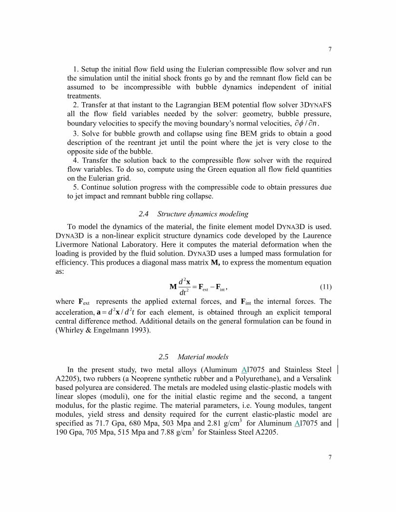
FIGURE 11 shows a time sequence of the contours of the von Mises equivalent

stresses in the material for one of the two metallic alloys considered here, AL7075. It is

seen that high stresses appear at the plate center near the surface when the reentrant jet

impact pressure reaches the wall at t - tlink = 0.2 s. The high stress wave is observed to

propagate and move radially away from the impact location. As the first high stress

wave starts to attenuate, another high stress is observed initiating from the top center of

the plate at t - tlink = 0.9 s, time at which the high pressure wave generated by the

collapse of the remaining bubble ring reaches the wall (see FIGURE 6f). It is interesting

r z

o

17

17

to note that the speed of stress wave propagation in the longitudinal direction (along the

axis of symmetry) is about 3,700 m/s, i.e. significantly smaller than the

expected 6,400 m/s longitudinal wave speed in AL7075. This is due to the plastic

deformation of the material, which modifies the material properties and wave behavior.

All high stresses due to the bubble dynamics eventually attenuate. However, residual

stresses remain below the plate surface due to the plastic deformations of the material.

In the conditions of FIGURE 11, these have their highest value occurring at a depth of 0.2

mm below the surface as shown in Figure 11f. Since the material is modeled as elastic-

plastic, permanent deformation should occur wherever the local equivalent stresses

exceed the material yield point. With the yield stress of AL7075 being 503 MPa, all

regions that have seen the top red stress contour level shown in FIGURE 11 experience

permanent deformation due to either reentrant jet impact or bubble ring collapse.

FIGURE 11. Time sequence of the equivalent stress contours in the Al7075 plate for

R0 = 50 μm, Rmax = 2.0 mm, Pd = 10 MPa, and 0.75X .

To quantitatively examine the material response to the pressure loading, the time

histories of the liquid pressure and the vertical displacement of the material surface at

the center of the Al7075 plate / liquid interface are shown together in FIGURE 12. The

material starts to get compressed as the high pressure loading due to the reentrant jet

impact reaches it, and the plate surface center point starts to move in at

t - tlink = 0.45 s. The maximum deformation occurs when the highest pressure loading

(a) t-tlink=0.2 s (b) t-tlink=0.4 s (c) t-tlink=0.6 s

(d) t-tlink=0.7 s (e) t-tlink=0.9 s (f) t-tlink=4.0 s

18

peak due to the bubble ring collapse reaches the center of the plate at time

t - tlink = 1.15 s. Once the pressure loading due to the full bubble dynamics has virtually

vanished at t - tlink = 4 s, the surface elevation continues to oscillate due to stress waves

propagating back and forth through the metal alloy thickness and lack of damping in the

model. Finally, a permanent deformation (pit) remains as a result of the high pressure

loading causing local stresses that exceed the Al7075 elastic limit. As shown in the

FIGURE 12, the vertical displacement of the monitored location eventually converges to

a non-zero value (~9m).

FIGURE 12. Time history of pressure and vertical displacement monitored at the center

location of the Al7075 plate top surface following the collapse of a cavitation bubble

near the plate for R0 = 50 μm, Rmax = 2.0 mm, Pd = 10 MPa, and 0.75X .

19

19

FIGURE 13. Profile of the permanent deformation an Al7075 plate surface following the

collapse of a cavitation bubble for R0 = 50 μm, Rmax = 2.0 mm, Pd = 10 MPa, and

0.75X .

The radial extent of the permanent deformation is shown in FIGURE 13. The profile

of the permanent deformation generated on the plate surface reproduces that of the

observed pit shapes (Philipp and Lauterborn 1998, Kim et al. 2014). To further study the

effect of different parameters on pit formation, we define in the following the pit depth

and the pit radius based on the pit profile as follows: the pit depth is the permanent

deformation measured at the center location of the plate / liquid interface and the pit

radius is the radial location where the vertical displacement is smaller than 1 μm.

3.5 Effect of Standoff on Pressure Loading and Material Deformation

It is known from previous studies on an explosion bubble near a rigid wall (Chahine

1996; Chahine et al. 2006, Jayaprakash et al. 2012) that the impact pressure due to the

reentrant jet attains a maximum at distances of the order of three quarters of the

maximum bubble radius, i.e. 𝑋 ̅= 0.75. In those studies, the jet hits the wall almost at the

same time when reentrant jet touchdown occurs even though a small liquid film always

exists between bubble and wall. However, for the current study as shown in FIGURE 6

the jet touchdown occurs at a small distance away from the wall. The shock generated

by the jet touchdown needs to travel a distance and thus attenuates before reaching the

wall. To study the effect of a direct jet impact, a smaller standoff at 𝑋 ̅= 0.5 is

simulated. FIGURE 15 shows the pressure contours at six selected time. One can see

clearly that the reentrant jet directly impacts on the wall when the jet touchdown occurs

at t - tlink = 0.05 s. Similar to 𝑋 ̅= 0.75 case, the volume of the bubble ring remaining

after the jet touchdown continues to shrink and reaches a minimum at about t - tlink =

20

0.92 s. However, the high pressure shock generated by the bubble ring collapse

originates much closer to the wall as compared to the 𝑋 ̅= 0.75 case. This results in a

higher concentrated pressure loading at the plate center when the shock wave propagates

toward and reaches the axis at t - tlink = 1.1 s.

FIGURE 14. Pressure contours at different instances during the bubble collapse near the

wall for bubble initial radius R0 = 50 µm, the equivalent radius at maximum Rmax = 2

mm, the initial standoff �̅� = 0.5, and the collapse driving pressure Pd = 10 MPa.

FIGURE 15 shows the pressure versus time monitored at the plate center for different

standoff distances. It is seen that the pressure loading due to the jet impact is much

higher for 0.5X case because the jet directly impacts on the wall when it penetrates

the other side of the bubble. The higher pressure loading due to the direct jet impact and

later more concentrated pressure loading due to the ring collapse is expected to results in

a different pit shape on material surface. As shown in

Figure 16 the pit radius is smaller with 0.5X than with 0.75X , while the pit

depth is larger with 0.5X than with 0.75X because of the higher magnitude and

concentrated pressure loadings.

(a) t-tlink=0.05 s (b) t-tlink=0.30 s (c) t-tlink=0.70 s

(d) t-tlink=0.92 s (e) t-tlink=0.97 s (f) t-tlink=1.1 s

21

21

FIGURE 15. Pressure versus time at the center of the plate for different bubble plate

standoff distances for R0 = 50 m, Rmax = 2 mm, and Pd = 10 Mpa.

FIGURE 16. Comparison of pit shape between 0.5X and 0.75X for Al7075 for

R0 = 50 m, Rmax = 2 mm, and Pd = 10 MPa.

3.6 Effect of Material Compliance on Pressure Loading

As shown in FIGURE 9 the main pressure peaks can be attributed to the jet impact

and bubble ring collapse. It is expected that the magnitudes of these pressure peaks

depend on the level of deformation of the solid material because the pressure loading on

material is a result of full interaction between collapsing bubbles and responding

22

material. FIGURE 17 shows a comparison of the time histories of the collapse impulsive

load between a non-deformable wall and an Al7075 deformable plate at the moment

when the initial shock wave reaches the wall. The figure shows that the pressure peak

felt by the wall is smaller when the solid boundary deforms and absorbs part of the

energy.

FIGURE 17. Comparison of time history of impact pressure between rigid wall and

Al7075 deformable plate near the moment as the initial shock wave reaching the wall

for 0.75X , R0 = 50 µm, Rmax = 2 mm, and Pd = 10 MPa.

To further study the effect of material compliance on the pressure loading we also

simulated the cavitation bubble dynamics near other compliant materials with the

properties described in Section 2.5 in addition to the metallic materils. Due to the low

compressive and shear strength of the considered compliant materials, a smaller collapse

driving pressure, Pd = 0.1 MPa, was chosen to avoid numerical issues caused by overly

squeezed elements with the large Pd used with the metallic allows. The other conditions

for the bubble dynamics presented for the base case were maintained. FIGURE 18a shows

the comparison of overall time histories of the pressures on a rigid fixed plate and four

other materials, i.e. A2205, Al7075, Rubber#2 and Versalink. FIGURE 18b shows the

detailed comparison of the pressure peaks due to the bubble ring collapse. From the

comparison it is seen that the impact pressures for the metallic alloys and the rigid plate

are very close. On the other hand, due to absorption of some energy through

deformation, lower magnitude of the impact pressures is seen on the softer materials.

This was already observed experimentally by Chahine and Kalumuck (1998b). Also, a

delay in the peak timing indicates that a soft material tends to elongate the bubble period

as compared to the rigid material. Such effect on bubble dynamics is similar to the free

surface vs solid wall.

23

23

FIGURE 18. a) Overall time history of the pressure at the plate center and b) zoom near

the pressure peaks due to ring collapse, for a rigid wall, two metallic alloys, and two

compliant materials for R0 = 50 m, Rmax = 2 mm, Pd = 0.1 MPa and 0.75.X

4 Tandem Cavitation Bubbles Collapse near Wall

Although cavitation is usually induced by external pressure variation in the flow

field, the resulting cavitation bubble dynamics is similar to that of underwater explosion

bubble or laser-induced cavitation bubble in which an initial high gas pressure bubble

undergoes explosive growth and violent collapse while the external pressure remains

constant. In this section we set up a tandem bubble case with both bubbles initially

containing high a gas pressure inside. Figure 19 illustrates the problem setup for the

tandem bubble case. Two bubbles are initially sitting above the plate at a standoff while

they are separate at a distance of D. The initial bubble radius is R0 = 50 m and the

initial gas pressure is specified such that the bubble will grow to a maximum size Rmax =

2 mm in a free field alone.

Figure 19. Illustration of problem setup for tandem bubble near a wall.

Ring

collapseJet impact

R0 = 50 µm

Standoff X

Spacing D

24

Here we study only the effects of bubble spacing D on the pressure loading and pit

shapes while the standoff is fixed at 0.75 Rmax. Three different values of bubble spacing,

i.e D=0.5, 1.5 and 2.5 Rmax are simulated and studied. Figure 20 shows tandem bubble

shapes for three different values of bubble spacing at the time before jet touches down.

It is seen that unlike the single bubble collapse near the wall the reentrant jet of the

tandem bubble collapse forms an angle deviated from perpendicular to wall due to

bubble and bubble interaction. If the two bubbles are equal, then an imaginary wall can

be assumed between the two bubbles. As a result, the angle of the reentrant jet is

controlled by both real and imaginary walls. If no viscosity is taken into account, both

walls impose a same effect on the bubble dynamics. As a result, when the spacing D is

twice of the standoff X, a 45 degree angle can be observed. For a smaller bubble spacing

the reentrant jet will first impact on the imaginary wall (or the other bubble) while for a

large bubble spacing the reentrant jet will impact first on the real wall.

Figure 20. Tandem bubble shapes for three different values of bubble spacing 1) D=0.5

Rmax, 2) D=1.5 Rmax and c) D=2.5 Rmax at the time when jet is touchdown.

FIGURE 21 through FIGURE 23 shows the pressure contours at different instances

during the tandem bubble collapse near the wall for D = 0.5, 1.5 and 2.5 Rmax

respectively. It is seen from FIGURE 21 that a high pressure shock is generated along the

center axis above the wall when the reentrant jets from both bubbles impact each other.

The shock then moves down toward the wall along the center axis and imposes a high

pressure loading on the wall. However, one can see that the shock is significantly

attenuated before reaching the wall. For the opposite case, D = 2.5 Rmax, the shock is

generated first when the jet impacts on the wall. This shock then moves along the wall

surface toward the center axis. Since the high pressure is acting on the wall while

moving toward the center, it is expected that the pressure loading on the wall would be

higher than the D = 0.5 Rmax case. For the D = 0.5 Rmax case, the bubble surface pinches

before the main jet front touches down. However, a final focused pressure loading is

found on the plate center.

25

25

FIGURE 21. Pressure contours at different instances during the tandem bubble collapse

near the wall for D = 0.5 Rmax.

FIGURE 22. Pressure contours at different instances during the tandem bubble collapse

near the wall for D = 1.5 Rmax.

FIGURE 23. Pressure contours at different instances during the tandem bubble collapse

near the wall for D = 2.5 Rmax.

26

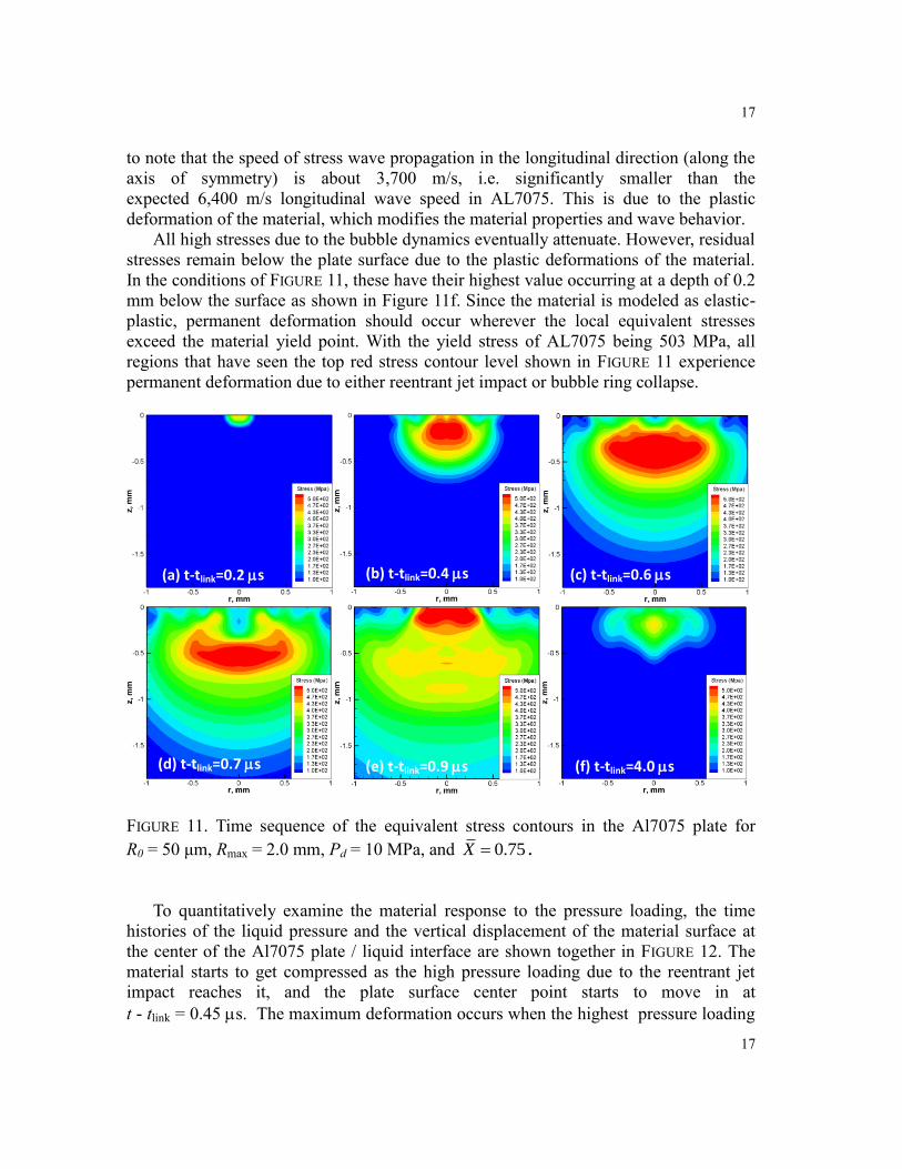
The quantitative comparison of the time history of pressure loading on the plate

center is shown in FIGURE 24. It is seen that the D = 1.5 Rmax case results in a highest

pressure loading at the center of plate. FIGURE 25 shows the comparison of the final pit

shapes for the three cases. It is seen that the D = 1.5 Rmax results in a deepest pit because

of the highest concentrated loading at the center of plate. However, the D = 2.5 Rmax

results in a wider pit because of a high pressure loading traveling across the wall

surface.

FIGURE 24. Comparison of time history of the pressure at the plate center for different

bubble spacing D.

27

27

FIGURE 25. Comparison of pit shape between for difference bubble spacing.

5 Bubble Cloud Collapse near Wall

So far we have addressed the cavitation bubble interaction with the material surface.

In this section, we will discuss the behavior of cloud of bubbles interacting with the

material. A 3D computational domain, which is 100 mm wide and 50 mm tall, as shown

in Figure 26 is prepared with two planes of symmetry (xz and yz-planes). On the z-axis

where the two symmetry planes intersect, a bubble with high pressure (25 atm) is

located away from the bottom wall, which is a 6 mm thick polyurea (Versalink)

material. The bubble with 25 atm initial gas pressure placed in 1 atm ambient pressure is

used as an excitation source in this problem, and the response of the bubble cloud

composed of 100 µm radius bubbles located near the wall will be observed. The bubbles

in the cloud are initially in equilibrium in the 1 atm ambient pressure. At far field, no

reflection boundary condition is applied.

Figure 27 shows the case of 90 bubbles in the cloud. The radius of bubbles in the

cloud is 100 µm, and the finest mesh size of 25 µm is used near these bubbles. A total of

4.7 million cells are used to model the problem. Figure 28 shows the pressure field near

the bubble cloud at the beginning of the dynamics. The bubble cloud first acts as a

shield preventing the shock wave generated by the excitation source from reaching the

wall. This is shown well in Figure 28 (b) where the high pressure (red region) impacted

the wall already outside the bubble cloud, but the pressure under the bubble cloud is still

close to the initial 1 atm. The bubbles in the outer edge of the cloud begin to collapse

28

first, and then the phenomenon propagates inward to the center of the bubble cloud.

After all, the bubbles in the cloud go through multiple collapse-rebound cycles, which

generate multiple pressure pulses in the region.

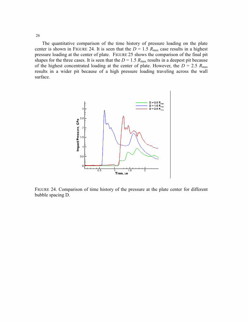
Figure 29 shows the time history of the radii of a few selected bubbles in the cloud.

Overall the bubbles in the cloud behave in unison, and the collapse and rebound are

almost at the same time. The first collapse is the strongest as this brings the bubbles to

their smallest size during their history. In Figure 29, another set of curves obtained with

150 µm bubbles in the cloud are shown for comparison. The overall trend looks the

same that the bubbles collapse and rebound in unison. Since the characteristic Rayleigh

time of a larger bubble is longer, the collapse of the 150 µm bubble cloud takes much

longer than the collapse of the 100 µm bubble cloud. Figure 30 shows the corresponding

pressure time history at the center on the material surface. As expected from the bubble

behavior shown in Figure 29, the first peak from the collapse of 100 µm bubbles occurs

earlier than the first peak for the 150 µm bubbles. Since the collapse of 150 µm bubbles

is stronger, the pressure peak of the 150 µm bubbles is much higher than that of the 100

µm bubbles.

FIGURE 26. Bubble cloud material interaction problem setup in DYSMAS. A side view

of the half domain is shown.

29

29

Figure 27. Computational mesh around the bubble cloud. The bubble radius is 100 µm,

and the finest mesh size of 25 µm is used near the bubbles. A total of 4.7 million cells

are used to model the problem.

FIGURE 28. The pressure fields near the bubble cloud at two different times; (a) t = 10

µs, (b) t = 20 µs. Bubble cloud acts as a shield first.

(a) (b)

30

Figure 29. Time history of the radii of bubbles in the cloud. Two different cases of initial

bubble radii, 100 µm and 150 µm, are compared.

Figure 30. Time history of the pressure at the center on the material surface. Two

different cases of initial bubble radii, 100 µm and 150 µm, are compared.

Similar computations were conducted with different number of bubbles in the cloud.

Figure 31 shows the pressure time histories at the center on the material obtained with

different number of bubbles in the cloud. It can be observed that the first collapse of the

bubble cloud is delayed and the pressure peak increases as the number of bubbles in the

31

31

cloud increases. This is the case for both kinds of simulations; one with rigid wall and

the other with compliant Versalink wall. The bubble cloud works as an energy

accumulator; the energy in the shock wave is absorbed by the bubble cloud, and then the

bubbles collapse at a later time. A larger cloud with larger number of bubbles

accumulates more energy and then generates larger pressure peak at the collapse of the

cloud. A larger cloud also takes longer from the time it is first exposed to the incoming

shock wave to the collapse, thus accumulating more energy in it.

Figure 32 shows only four curves selected from Figure 31. The pressure peaks with

the rigid wall are observed to be 2-3 times higher than those with the compliant wall. In

case of compliant wall, the wall sinks in when the high pressure impacts the wall. This

fluid-structure interaction reduces the pressure peaks because part of the energy from

the shock wave is absorbed by the compliant material as the material deforms. This has

an implication in the cavitation erosion of compliant materials, which we are currently

studying further.

Figure 31. Effect of number of bubbles and the wall material on the pressure generated

by the bubble cloud collapse.

32

Figure 32. Comparison of the wall pressure due to 1 bubble and 74 bubbles.

6 Conclusions

Material pitting due to cavitation bubble collapse is studied by modeling the

dynamics of growing and collapsing cavitation bubble near a deforming material with

an initial flat surface. The pressure loading on the material surface during the bubble

collapse is found to be due to the reentrant jet impact and to the collapse of the

remaining bubble ring. The high pressure loading results in high stress waves, which

propagate radially from the loading location into the material and cause the deformation.

A pit (permanent deformation) is formed when the local equivalent stresses exceed the

material yield stress.

The loading is highly dependent on the standoff distance. The initial standoff

distance between the bubble and the material affects the jet characteristics in a non-

monotonic fashion. Higher jet velocities occur at the larger standoff distances. However,

the energy in the jet is maximum at a normalized standoff distance close to X = 0.75. A

higher jet velocity does not necessarily result in a higher impact pressure, since the

impact pressure also depends on the distance between the wall and the jet front at the

touchdown moment. A more concentrated pressure loading on the material surface is

obtained for smaller standoffs where the jet touches downs and the bubble ring collapses

very close to the wall. Such concentrated pressure loadings result in deeper but narrower

pits. As a result, the shape of the pit, i.e. the ratio of pit radius and depth does not vary

monotonically with standoff.

The magnitude of the pressure peaks felt by the material depends on the response

and amount of deformation of the solid. The fluid structure interaction simulations show

that the load on the material is reduced and this reduction increases when the solid

boundary deformation increases and more energy is absorbed. From the study of

33

33

different material types, it was found that material response has a strong effect on the

impact pressures due to strong fluid structure interaction. Impact pressures for metallic

alloys are very close to those on a rigid plate while compliant materials deform and

absorb energy. This results in lower magnitude of the impact pressures and delays in

peak occurrence due to lengthening of the bubble period.

Acknowledgements

This work was conducted under support from DYNAFLOW, INC. internal IR&D and

partial support from the Office of Naval Research under Contract N00014-12-M-0238,

monitored by Dr. Ki-Han Kim. We would also like to thank Gregory Harris from the

Naval Surface Warfare Center, Indian Head, for allowing us access to the GEMINI code

and contribution to its coupling to the DYNA3D Structure code. Their support is greatly

appreciated.

REFERENCES

Amirkhizi, A.V., Isaacs, J., McGee, J. & Nemat-Nasser, S. 2006 An experimentally-

based viscoelastic constitutive model for polyurea, including pressure and

temperature effects. Philosophical Magazine, 86 (36), 5847-5866.

Anderson, J.D. 1990 Modern compressible flow: with historical perspective. Vol. 12.

McGraw-Hill New York.

Besant, W. H. 1859. A treatise on hydrostatics and hydrodynamics. Deighton, Bell.

Blake, J.R. & Gibson, D.C. 1987 Cavitation bubbles near boundaries. Ann. Rev. Fluid

Mech., 19, 99-124.

Brayman A.A., Azadniv, M., Cox, C., Miller, M. W., 1999 Erosion of artificial

endothelia in vitro by pulsed untrasound: acoustic pressure, frequency,

membrane orientation and microbubble contrast agent dependence, Ultrasound

in Med. & Biol. 25, 1305-1320.

Brennen, C.E. 1995 Cavitation and Bubble Dynamics. New York, Oxford University

Press, Chahine GL, Hsiao C-T, Raju R (2013) Scaling of cavitation bubble cloud

dynamics on propellers. In Kim KH, Chahine GL, Franc J-P, Karimi A (eds.)

Advanced Experimental and Numerical Techniques for Cavitation Erosion

Prediction, Series Fluid Mechanics and Its Applications, Springer

Chahine G.L. 1982 Experimental and asymptotic study of nonspherical bubble collapse.

Applied Scientific Research, 38, 187-197.

Chahine, G.L., Conn, A.F., Johnson, V.E., and Frederick, G.S., 1983 "Cleaning and

Cutting with Self-Resonating Pulsed Water Jets", 2nd US Water Jet Conference,

Rolla, Missouri, May 24-26.

34

Chahine, G.L. & Shen, Y.T. 1986 Bubble dynamics and cavitation inception in

cavitation susceptibility meter. ASME Journal of Fluid Engineering, 108, 444-

452.

Chahine, G.L. & Perdue, T.O. 1989 Simulation of the three-dimensional behavior of an

unsteady large bubble near a structure. 3rd International Colloquium on Drops

and Bubbles, Monterey, CA, Sept.

Chahine, G.L. 1993 Cavitation dynamics at microscale level. Journal of Heart Valve

Disease, 3, 102-116.

Chahine G. L., Duraiswami, R. and Kalumuck, K.M. 1996 Boundary element method

for calculating 2-D and 3-D underwater explosion bubble loading on nearby

structures. Naval Surface Warfare Center, Weapons Research and Technology

Department, Report NSWCDD/TR-93/46, September (limited distribution).

Chahine, G.L. & Kalumuck, K.M. 1998a BEM software for free surface flow simulation

including fluid structure interaction effects. Int. Journal of Computer Application

in Technology, Vol. 3/4/5.

Chahine, G.L., and Kalumuck, K.M. 1998b The Influence of Structural deformation on

Water Jet Impact Loading, Journal of Fluids and Structures, Vol. 12, (1), pp.

103-121, Jan.

Chahine G.L., Annasami R., Hsiao C.-T. & Harris G. 2006 Scaling rules for the

prediction on UNDEX bubble re-entering jet parameters. SAVIAC Critical

Technologies in Shock and Vibration, 4 (1), 1-12.

Chahine, G.L. 2014 Modeling of Cavitation Dynamics and Interaction with Material,

Chap. 6 in Advanced Experimental and Numerical Techniques for Cavitation

Erosion Prediction Editors Kim, K.H., Chahine, G.L., Franc, J.P., & Karimi, A.,

Springer.

Cravotto, G., Boffa, L., Mantegna, S., Perego, P., Avogadro, M., & Cintas, P. 2008

Improved extraction of vegetable oils under high-intensity ultrasound and/or

microwaves. Ultrasonics Sonochemistry, 15(5), 898-902.

Colella, P. 1985 A direct Eulerian MUSCL scheme for gas dynamics. SIAM Journal on

Scientific and Statistical Computing, 6(1): 104-117.

Crum L.A., 1979. Surface Oscillations and jet development in pulsating bubbles.

Journal de Physique, colloque c8, supplément au N. 11, tome 40, c8-285.

Dalecki, D., Child, S.Z., Raeman, C.H., Xing, C., Gracewski, S., Carestensen, E. L.,

2000 Bioeffects of positive and negative acoustic pressures in mice infused with

microbubbles, » Ultrasound in Med & Biol. 26, 1327-1332.

Duncan, J.H., Milligan, C.D. & Zhange, S. 1991 On the interaction of a collapsing

cavity and a compilant wall. J. Fluid Mech. 226, 401-423.

Duncan, J.H., Milligan, C.D. & Zhang, S. 1996 On the interaction between a bubble and

submerged compliant structure. J. Sound & Vibration, 197, 17-44.

Harris, G.S., Illamni, R., Lewis, W., Rye, K., and Chahine, G.L. 2009 Underwater

Explosion Bubble Phenomena Tests Near a Simulated Dam Structure", Naval

Surface Warfare Center - Indian Head Division, IHTR 10-3055, Nov. 1.

35

35

Hsiao, C.-T. & Chahine, G.L., 2010 Incompressible-compressible link to accurately

predict wall Pressure. 81th

Shock and Vibration Symposium, Orlando, FL,

October 24-28.

Hsiao, C.-T. & Chahine, G.L. 2013a Development of compressible-incompressible link

to efficiently model bubble dynamics near floating body. Advances in Boundary

Element & Meshless Techniques XIV, pp. 141-152.

Hsiao, C.-T. & Chahine, G.L. 2013b Breakup of finite thickness viscous shell

microbubbles by ultrasound: a simplified zero thickness shell model. J. Acoust.

Soc. Am., 133 (4), 1897-1910.

Jayaprakash, A., Hsiao, C.-T. & Chahine, G.L. 2012 Numerical and experimental study

of the interaction of a spark-generated bubble and a vertical wall. ASME Journal

of Fluids Engineering, 134, 031301,

Jones , I.R. and Edwards, D.H., 1960 An experimental study of the forces generated by

the collapse of transient cavities in water, J. Fluid Mech., 7, 596-609.

Kalumuck, K.M., Duraiswami, R. & Chahine, G.L. 1995 Bubble dynamics fluid-

structure interaction simulation on coupling fluid BEM and structural FEM

codes, Journal of Fluids and Structures, 9, 861-883. Kalumuck, K.M., Chahine, G.L. & Hsiao, C.-T. 2003 Simulation of surface piercing

body coupled response to underwater bubble dynamics utilizing 3DYNAFS

, a

three-dimensional BEM code. Computational Mechanics, 32, 319-326

Kalumuck, K. M., & Chahine, G. L. 2000. The use of cavitating jets to oxidize organic

compounds in water. Journal of Fluids Engineering, 122(3), 465-470.

Kapahi, A., C.-T. Hsiao, and G.L. Chahine., A multi-material flow solver for high speed

compressible flow applications, to appear in Computers & Fluids, 2014.

Kim, K.H., Chahine, G.L., Franc, J.P., & Karimi, A. 2014 “Advanced Experimental and

Numerical Techniques for Cavitation Erosion Prediction”, ISBN: 978-94-017-

8538-9 (Print) 978-94-017-8539-6 (Online), Springer.

Key, S.W. 1974 HONDO- A finite element computer program for the large deformation

dynamics response of axisymmetric solids. Sandia National Laboratories,

Albuquerque, N.M, Report. 74-0039.

Madadi-Kandjani, E., Xiong, Q., 2014 Validity of the spring-backed membrane model

for bubble-wall interactions with compliant walls. Computers & Fluids, doi:

http://dx.doi.org/10.1016/j.compfluid.2014.03.010

Naude, C.F. & Ellis, A.T. 1961 On the mechanism of cavitation damage by non-

hemispherical cavities collapsing in contact with a solid boundary. ASME J.

Basic Engineering, 83, 648-656.

Philipp, A. & Lauterborn W., 1998 Cavitation erosion by single laser-produced bubbles.

J. Fluid Mech., 361, 75-116.

Plesset, M.S. & Chapman, R.B. 1971 Collapse of an initially spherical vapour cavity in

the neighborhood of a solid boundary. J . Fluid Mech. 47, part 2, 283-290.

Rayleigh, Lord, 1917 On the pressure developed in a liquid during the collapse of a

spherical cavity. Phil. Mag. 34, 94-98.

36

Sankin, G.N., Yuan, F., Zhong, P., 2010 Pulsating Tandem Microbubble for Localized

and Directional Single Cell Membrane Poration,” Phys. Rev. Lett., 105 (7).

Vogel, A. & Lauterborn W., 1988 Acoustic transient generation by laser-produced

cavitation bubbles near solid boundaries. J. Acoust. Soc. Am., 84, 719-731.

Wang, Q. X. and Blake, J. R. 2010 Non-spherical bubble dynamics in a compressible

liquid. Part 1. Travelling acoustic wave. J. Fluid Mech. 659, 191-224.

Wang, Q. X. and Blake J. R. 2011 Non-spherical bubble dynamics in a compressible

liquid. Part 2. J. Fluid Mech. 679, 559–581.

Wang, Q. X. 2013 Underwater explosion bubble dynamics in a compressible liquid.

Phys. Fluids 25, 072104.

Wardlaw, A.B. Jr. & Luton, A.J, 2000 Fluid structure interaction for close-in explosion.

Shock and Vibration, 7, 265-275.

Wardlaw, A.B., Luton, J.A., Renzi, J.R., Kiddy, K.C. & McKeown, R.M. 2003 The

Gemini Euler solver for the coupled simulation of underwater explosions. Indian

Head Technical Report 2500, November.

Whirley, R.G. & Engelmann, B.E., 1993 DYNA3D: A nonlinear, explicit, three-

dimensional finite element code for solid and structural mechanics – user

manual. Lawrence Livermore National Laboratory, Report UCRL-MA-107254

Rev. 1, November.

Zel'Dovich, Y.B. & Y.P. Raizer, 2002 Physics of shock waves and high-temperature

hydrodynamic phenomena. Dover Pubns.

Zhang S., Duncan J. H. & Chahine G. L. 1993 The final stage of the collapse of a

cavitation bubble near a rigid wall. J. Fluid Mech., 257, 147-181.