MODELING C:N RATIO FOR THE COMPOSTABLE SOLID WASTES

USING ARTIFICIAL NEURAL NETWORKS

Adem BAYRAM a*, Murat KANKAL a, Talat Sukru OZSAHIN a, Fatih SAKA b

a Karadeniz Technical University, Faculty of Engineering, Department of Civil Engineering,

61080 Trabzon, Turkey

b Gümüşhane University, Faculty of Engineering, Department of Civil Engineering,

29000 Gümüşhane, Turkey

Corresponding author. Tel.: +90 462 377 41 73; fax: +90 462 377 26 06

E-mail address: adembayram@gmail.com (A. BAYRAM)

1

Abstract

Organic wastes constitute a major part of municipal solid wastes (MSWs), and they cause to

some unwanted problems both at open dumps, sanitary landfills and incineration plants.

Composting is one element of an integrated solid waste management strategy that can be

applied to mixed collected MSWs or to separately collected leaves, yard wastes and food

wastes. The most critical environmental factor for composting is the carbon to nitrogen (C:N)

ratio. In this study, two analysis methods being multi linear regression analysis (LRA) and an

artificial neural network (ANN) analysis were applied to predict C:N ratio of compostable

part of the MSWs. Experimentally determined seven variables belonging to the solid waste

samples taken from the MSW open dumping area in Gümüşhane Province, Turkey, were used

for the prediction of C:N ratio in the analyses. Two of these variables were percentages of

food and yard (F&Y), and ash and scoria (A&S) obtained by the way of sorting process of

Gümüşhane MSWs. Five of these variables were moisture content (MC), fixed carbon (FC)

content, total organic matter (TOM) content, high calorific value (HCV) and pH of

compostable part of the MSWs. There were 52 data for every variable. 42 of the data were

used for training set, and the rest of the data were used for testing set in the ANN analysis. As

the results of analyses, the smallest average relative error value for testing set obtained from

ANN methods was 6.376 %, but it was 11.002 % for LRA. The effects of TOM content, F&Y

percentage and A&S percentage values on the C:N ratio were also investigated by simulating

the ANN model for different values of these variables. It was concluded that ANN analysis

used for estimation of the C:N ratio provided reasonable results.

Keywords: Artificial neural network, C:N ratio, Municipal solid waste, Composting

2

1. Introduction

Municipal solid waste (MSW) is generated and accumulated as the result of human activities.

The waste will cause serious environmental pollution unless a proper solid waste management

system is applied. One of the most traditional and popular disposal methods for MSW,

particularly in developing countries is landfilling. However, this type of technology should be

improved and substituted by other processes due to the limited land area in some countries

and due to some environmental problems associated with the landfilling process, such as gas

emissions and leachate production [1].

Organic wastes constitute a major part of municipal solid waste. They cause some unwanted

problems both at open dumps, sanitary landfills and incineration plants. Some of the problems

at open dumps or sanitary landfills are leachate, which have polluting potential for

groundwater and superficial water sources, generated as a result of degradation and

decomposition of organic materials, uncontrolled release of landfill gases, which may cause

serious health problems when inhaled, such as hydrogen sulfur (H2S), carbon dioxide (CO2)

and methane (CH4). Some of the problems in incineration are that additional fuel is needed

due to the fact that organic materials have high moisture content and low calorific value, and

air pollution, which is caused by some unwanted gases generated as a result of incineration.

There are solutions for these problems but increase the cost to a great degree. The studies

were started in order to produce economical and environment-friendly solutions for these

problems together with municipal solid waste management. In the end, the opinion of utilizing

organic waste as a soil conditioner or fertilizer by composting appeared. Composting was

accepted and put into practice as a solid waste disposal alternative to open dumping or sanitary

landfilling [2].

3

Composting is one element of an integrated solid waste management strategy that can be

applied to mixed municipal solid waste (MSW) or to separately collected leaves, yard wastes,

and food wastes [3]. It is the biological decomposition of the biodegradable organic fraction of

MSW under controlled conditions to a state sufficiently stable for nuisance-free storage and

handling and for safe use in land applications [4,5].

The most critical environmental factor for composting is the C:N ratio. In general, an initial

C:N ratio of 30:1 is considered ideal. When the C:N ratio is greater than 35:1, the composting

process slows down. When the ratio is less than 25:1, there can be odor problems due to

anaerobic conditions, release of ammonia, and accelerated decomposition. As the composting

process proceeds and carbon is lost to the atmosphere, this ratio narrows. Finished compost

should have a C:N ratio of 15:1 to 20:1 [6].

Carbon is oxidized to produce energy and metabolized to synthesize cellular constituents.

Nitrogen is an important constituent of protoplasm, proteins, and amino acids. An organism

can neither grow nor multiply in the absence of nitrogen in a form that is accessible to it.

Although microbes continue to be active without having a nitrogen source, the activity rapidly

dwindles as cells age and die [3].

Artificial neural networks (ANNs) have an inherent ability to learn and recognize highly

nonlinear relationships [7], and then organize dispersed data into a nonlinear model [8]. Thus,

they provide an ideal means to predict C:N ratio of MSW. ANN has been applied in some

areas related to MSW; Dong et al. [1] predicted the heating value of MSW with a feed

forward neural network, Shu et al. [9] also predicted energy contents of Taiwan MSW using

multilayer perceptron neural networks, and Xiao et al. [10] predicted the gasification

characteristics of MSW applying ANN. Also, Jalili and Noori [11] proposed an appropriate

model for predicting the weight of waste generation in Mashhad with application of feed

4

forward artificial neural network and Noori et al. [12] conducted comparison of neural

network and principal component - regression analysis to predict the solid waste generation in

Tehran.

Ito et al. [13] developed an ANN model to predict the net nitrification potential of the forest

soils using two soil properties, C:N ratio and the maximum water-holding capacity. ANNs

have also been successfully used tools in the fields of water quality prediction and forecasting.

Moatar et al. [14] applied ANNs to estimate the daily pH of the Middle Loire River. FNN

models were identified, validated and tested for the computation of DO (dissolved oxygen)

[15], and DO and BOD (biochemical oxygen demand) [16] of river water.

This study especially focused on the ANN technique for predicting C:N ratio of compostable

part of the MSW generated in the city of Gümüşhane based on the variables being food and

yard percentage, ash and scoria percentage from the MSW components, and moisture content,

fixed carbon content, total organic matter content, high calorific value and pH from the

compostable part. The data were experimentally obtained on a weekly basis during March

2004 and February 2005, and the analyses were performed by using these 52 weeks

laboratory data set. It was determined that ANN technique yielded better results by

comparison with regression analysis. Finally, the network was simulated by using some

unknown data and effects of the variables such as A&S and TOM on C:N ratio.

2. Artificial neural network (ANN) approach

ANNs are human attempts to simulate and understand what goes on in nervous system, with

the hope of capturing some of the power of these biological systems. ANNs are inspired by

biological systems with large number of neurons which collectively perform tasks that even

the largest computers have not been able to match.

5

The function of artificial neurons is similar to that of real neurons; they are able to

communicate by sending signals to each other over a large number of biased or weighted

connections. Each of these neurons has an associated transfer function which describes how

the weighted sum of its input is converted to an output (Fig. 1).

Take in Figure 1

Different types of ANNs have evolved based on the neuron arrangement, their connections

and training paradigm used. Among the various type of ANNs, the multi-layer perceptron

(MLP) trained with back propagation algorithm has been proved to be most useful in

engineering applications. Back propagation is a systematic method for training multi-layer

perceptron.

The multi-layer perceptron network comprises an input layer, an output layer and a number of

hidden layers (Fig. 2). The presence of hidden layers allows the network to present and

compute more complicated associations between patterns. Basic methodology of ANNs

consists of two processes; network training and testing.

Take in Figure 2

The connection weights of the ANN are adjusted through the training process, while training

effect is referred to as supervised learning. The training of ANNs usually involves modifying

connection weights by means of learning rule. The learning process is done by giving weights

and biases computed from a set training data or by adjusting weights according to a certain

condition. Then, other testing data are used to check the generalization. The initial weights

and biases are commonly assigned randomly. As input data are passed through hidden layers,

sigmoidal activation function is generally used. During the training procedure, the data are

6

selected uniformly. A specific pass is completed when all data sets have been processed.

Generally, several passes are required to attain a desired level of estimation accuracy.

Training actually means for each input pattern and then compares it with the correct output.

The total error based on the squared difference between predicted and actual output is

computed for the whole training set. The adjustment of the corrections weights has been

carried out using the standard error back propagation algorithm, which minimizes the total

error (E) with the gradient decent method [17,18].

The back-propagation algorithm is given briefly as follows:

Step 0. Initialize weights: To small random values,

Step 1. Apply a sample: Apply to the input a sample vector uk having desired output vector yk,

Step 2. Forward phase: Starting from the first hidden layer and propagating towards the

output layer:

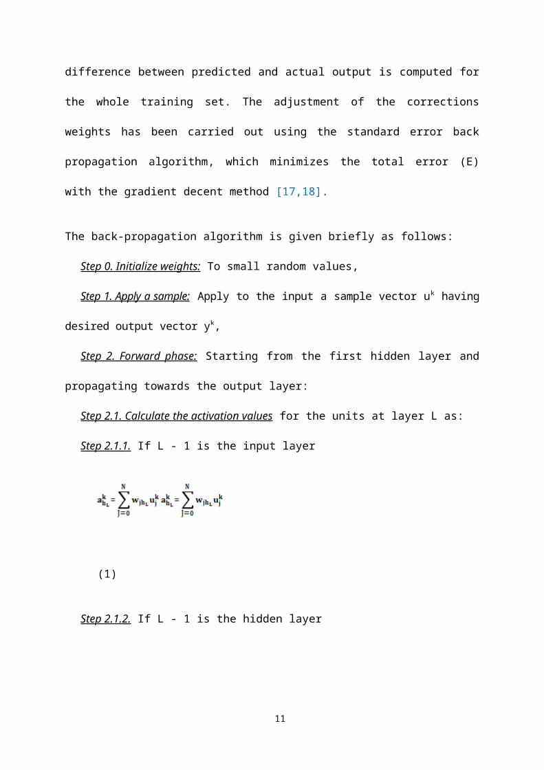
Step 2.1. Calculate the activation values for the units at layer L as:

Step 2.1.1. If L - 1 is the input layer

(1)

Step 2.1.2. If L - 1 is the hidden layer

(2)

Step 2.2. Calculate the output values for the units at layer L as:

(3)

7

where we use i0 instead of hL if it is an output layer, f is an activation function.

Step 3. Output errors: Calculate the error terms at the output layer as:

(4)

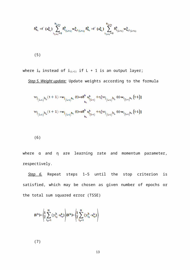
Step 4. Backward phase: Propagate error backward to the input layer through each layer L

using the error term

(5)

where i0 instead of i(L+1) if L + 1 is an output layer;

Step 5. Weight update: Update weights according to the formula

(6)

where α and η are learning rate and momentum parameter, respectively.

Step 6. Repeat steps 1–5 until the stop criterion is satisfied, which may be chosen as given

number of epochs or the total sum squared error (TSSE)

(7)

is sufficiently small [19]. The foregoing algorithm used in this study updates the weights after

an epoch is presented. Epoch is one cycle through the entire set of training patterns.

3. Study Area

8

Gümüşhane, located in the Eastern Black Sea Region of Turkey, lies between the 38° 45′ and

40° 12′ eastern longitudes and 39° 45′ and 40° 50′ northern latitudes. Gümüşhane is

characterized by a rugged topography. The area of Gümüşhane is some 6437 km2 at an

elevation of 1210 m. The lowest and highest elevations in the zoning plan are 1105 m and

1455 m, respectively. The temperature and other climatic conditions of Gümüşhane vary

drastically. According to temperature and rainfall data, containing 10 years of record between

1996 and 2005, collected from Turkish State Meteorological Service (TSMS) weather station

in Gümüşhane Province, the average minimum temperature is found to vary from -15°C in

February to 9°C in August, and the average maximum temperature is found to vary from 10°C

in January to 37°C in July. Gümüşhane receives a yearly average rainfall of 461 mm.

4. Materials and methods

4.1. Sampling and sorting process

The solid waste samples were taken from the MSW open dumping area (Fig. 3), Kurudere

valley in southwest side of Parmaklık hill (1633 m), for a year between March 2004 and

February 2005. Four samples were simultaneously taken in every week, and total two hundred

eight samples were taken in a year. Containers with 0.72 m3 capacity were used in the

sampling process. In order to obtain a representative sample, 0.288 m3 of the MSW was

collected. After the MSW was disposed of, the solid waste samples were taken promptly.

However, some materials having big volume, such as car tires, old house belongings and also

medical wastes were excluded. The collected samples were transported to an indoor area, the

solid wastes laboratory at Karadeniz Technical University, Gümüşhane Faculty of

Engineering. The samples were then spread out on a plastic sheet and manually separated into

their components. Sorting process was performed by a team of two people who were

instructed on the sorting requirements. The components were divided into nine categories:

9

food and yard (F&Y), paper and cardboard (P&C), metals, glass, plastics, textiles, ash and

scoria (A&S), diaper and others (wood, bones, battery, construction and demolition wastes,

stone, etc.). Each component was weighed and compared with the total [20].

Take in Figure 3

4.2. Sample processing (drying and grinding)

The compostable wastes were made reduced in size by pre-breaking and manually

homogenized in a plastic container. A sample of 4-5 kg sample was used for roughly

grinding. Four samples with 125 g were taken from roughly grinded homogenized

compostable wastes and dried in a drying oven for 24-48 h at 75°C until a constant weight

was obtained [21]. The dried samples being called dry matter (DM) were then placed into

desiccators for cooling and ground to obtain a particle size of less than 0.2 mm and stored in

desiccators until needed.

4.3. Analysis

The moisture content (MC) of the samples was determined from the decrease in weight. Total

organic matter (TOM) content of the dried matter was determined by igniting at 550°C in a

furnace [22]. The high calorific value (HCV) of dried solid wastes was determined with the

AC-350 calorimeter. The pH of the samples was determined with a mobile pH meter (pH

330i) according to EPA Method 9045D [23]. Total Organic Carbon (TOC) and Total Nitrogen

(TN) of the samples were determined with a UV-VIS spectrophotometer (Cadas 200) and its

cuvette-tests (TOC cuvette test measuring range 2-65 mg/l TOC and LATON TN cuvette test

measuring range 20-100 mg/l TN). Grinded samples were extracted according to EPA

Method 1310B [24] before the determination of TOC and TN. Determination principle of

TOC: Total carbon (TC) and total inorganic carbon (TIC) are converted to carbon dioxide

10

(CO2) by, respectively, oxidation and acidification. The CO2 passes from the digestion cuvette

through a membrane and into the indicator cuvette. The change of colour of the indicator is

photometrically evaluated. TOC is determined as the difference between the TC and TIC

values. Determination principle of TN: Inorganically and organically bonded nitrogen is

oxidized to nitrate by digestion with peroxodisulphate. The nitrate ions react with 2.6-

dimethylphenol in a solution of sulphuric and phosphoric acid to form a nitrophenol.

Experimental results belonging to all of the studied variables are given in Table 1 [25,26,27].

Take in Table 1

5. Analysis of the Sample Characteristics

5.1. Multi Linear Regression Model

Multi linear regression model is used for the prediction of C:N ratio (y), and the model as

follows:

y = a1 x1 + a2 x2 +a3 x3 + a4 x4 + a5 x5 + a6 x6 + a7 x7 + c (8)

where a1 - a7 and c are regression coefficients; x1 is F&Y percentage; x2 is A&S percentage; x3

is MC; x4 is FC; x5 is TOM; x6 is HCV and x7 is pH. The regression coefficient (R2) was

determined as 0.490 for the model (Table 2).

Take in Table 2

5.2. Construction, Teaching and Testing of Artificial Neural Network

The main objective of this section is to develop an appropriate ANN model for prediction of

the C:N ratio by training experimental data including F&Y percentage, A&S percentage, MC,

11

FC, TOM, HCV and pH. It is important to choose the proper network size. If the network is

too small, it may not be able to represent the system adequately. On the other hand, if the

network is too big, it becomes over trained and may provide erroneous results for untrained

patterns. In general, it is not straightforward to determine the best size of the networks for a

given system. As shown in Fig. 2, a three layer network is selected for the present study. Each

layer is connected to the next but no connections exist between neurons on the same level.

The number of neurons in the first and third layers, which contain input and output data

respectively, is predetermined and depends on the problem at hand. There are seven nodes in

the input layer corresponding to the seven variables and the C:N ratio (y) is in the output

layer. The variables in the input layers are the following: F&Y, A&S, MC, FC, TOM, HCV

and pH.

They are split into the training and testing patterns of the numbers 42 and 10, respectively.

Input values of the testing (test no 1, 5, 12, 14, 20, 26, 28, 32, 42 and 46) and training set can

be seen in Table 1.

Data preprocessing is also known as data normalization. Raw data need to be preprocessed

into a range that can be accepted by the network. Hyperbolic tangent sigmoid (input layer →

hidden layer) and logistic sigmoid (hidden layer → output layer) transfer functions are used

within the network. Scaling of the inputs to the range [0, 1] greatly improves the learning

speed. Therefore, each group of input and output values are normalized into range [0.1, 0.9]

as,

(9)

The definition of network size is a compromise between generalization and convergence.

Convergence is the capacity of the network to learn the pattern on the training set, and

12

generalization is the capacity to respond correctly to new patterns. The idea is to implement

the smallest network possible, so it is able to learn all patterns and at the same time provides

good generalization. As for the number of hidden layer, it is well said that one hidden layer is

sufficient for most usual applications, thus only one hidden layer is used in this study.

Determining the number of nodes to include in the hidden layer is not an exact science, so

network is tested for different number of hidden layer nodes. Parameters used to find

optimum ANN structures are given in Table 3. During the training process, all of the training

patterns are introduced to the network, and corresponding outputs are obtained. Then, the

network error (E) is computed according to Eq. (7) and the increments of generalized weights

are computed by Eq. (6). The choice of initial weights will influence the net reaches a global

minimum of the error and, if so, how quickly it converges. As mentioned earlier, the update of

the weight between two units depends on both derivative of the upper unit’s activation

function and activation of the lower unit. For this reason, it is important to avoid choices of

initial weights that would make it likely that either activations or derivatives of activations are

zero. In this study, the weights are initialized into random values between -0.5 and +0.5, a

procedure commonly accepted. Factors α and η in Eq. (6) also influence the convergence. The

learning rate (α) is the constant of proportionality of the generalized rule. The larger the value

is the greater the changes in weights. The momentum term (η) is used to smooth out the

weight changes to prevent network training from oscillating. Different combinations of

selected values of α and η are tried for good convergence of the neural network (Table 3).

Take in Table 3

The level of convergence in training is monitored using TSSE of training and testing patterns

separately. Training patterns were introduced to NN five times in each cycle as shown in the

4th column (cycle) in Table 4. The patterns are presented to each epoch in the same order.

13

After the learning set of data presented to the ANN models, we stopped the learning process

when the epochs reached to 100000, and determined which epoch number gives the minimum

TSSE of testing set for various ANN alternatives. Table 4 shows the structures of the ANN

giving the best results.

Take in Table 4

6. Results and Discussion

It is found that there is a tradeoff between the performance of a network and time consumed.

Generally, the performance of a network is found to increase with the suitable increase in the

number of samples, epochs (learning time) and the number of hidden layer nodes. Meanwhile,

the increase of these parameters also increases the consumed time. It may be said that,

learning rate (α) and momentum term (η) in addition to hidden layer nodes, epochs and

number of samples also influence the network to provide good generalization too much [28].

In the ANN analysis, the smallest average relative error value in the testing sets are obtained

from the network with α = 0.1 and η = 0.75 as 6.376 % (Table 4). The maximum relative error

of testing data set in this case is 9.528 %. Maximum relative error may be reduced if stopping

criteria, epoch number, is increased. Besides, conjugate gradient or scaled conjugate gradient

methods may be used to reduce maximum relative error instead of generalized delta rule in

learning. Also, different network structures with one or more hidden layers or nodes with

different learning rates and momentum terms may produce smaller error. Relative error is

calculated as

(10)

14

where OANN and Oreal are the computed and real values, respectively. Testing set is used to

evaluate the confidence in the performance of the trained network. Ten testing vectors are

used to test the ANN model. Fig. 4 is an expression of the learning results of network, and

each lozenge sign stands for a testing vector. Also, the results obtained from LRA for the

same values are shown with triangles in the same figure. The nearer the points gather around

the diagonal the better the learning results are. The relative errors of the points on the diagonal

are zero. Although the maximum relative error obtained from the testing set for ANN analysis

is 9.528 %, the maximum relative errors obtained from LRA are 31.294 %. Average relative

error of testing set of ANN analysis is 6.376 % while the average relative errors obtained

from LRA are 11.002 %. As a consequence, it is shown that ANN analysis, which is used for

the determination of C:N ratio, gives reasonable results.

Take in Figure 4

After training is accomplished, the network becomes able to respond upon unknown input. In

this way, the constructed network can be used to recognize and generate patterns given by

new inputs. The trained NN model is used to simulate the effect of TOM on the C:N ratio.

Effect of the variation in the TOM values on the C:N ratio is seen in Fig. 5. The changed

TOM values were obtained by adding a value with 4 % corresponding to the variation

coefficient, division of the standard deviation to the arithmetic average, to every TOM value

or by subtracting a value with 4 % from every TOM value. Evaluation was performed for

total 15 samples by starting from the 3rd sample with four-week intervals. The C:N ratio

increased together with increasing of the TOM value (Fig. 5).

Take in Figure 5

15

Effect of the changing in the A&S percentages on the C:N ratio was also investigated. The

A&S component was 0 % during the 14th and 33th weeks. The case that the A&S component

was also 0 % in the weeks after 33th week was simulated in the ANN model, and the variation

occurred in the C:N ratio was given in Fig. 6. A decrease occurred in the C:N ratio together

with decreasing of the A&S percentage. Conversely, the case that A&S percentage, which

was 0 % during the 14th and 33th weeks, was 41.5 %, which was average of the values in the

other weeks, was investigated, and the obtained results were given in Fig. 7. It was clearly

seen that the C:N ratio increased together with increasing of the A&S percentage.

Take in Figure 6

Take in Figure 7

Finally, effect of the changing in the F&Y percentages on the C:N ratio was investigated.

Evaluation was conducted between 14th and 33th weeks when the A&S component was 0 %. A

value with 40 % corresponding to the variation coefficient was added to the actual percentage

of the F&Y component or subtracted from this actual value. The obtained values were

simulated in the ANN and the results were given in Fig. 8. It was seen that C:N ratio

increased together with increasing of the percentage value of the F&Y component except for a

small number of sample.

Take in Figure 8

7. Conclusion

The most important scope of this study is to predict C:N ratio of compostable part of the

MSW using ANN. Training and testing patterns of neural network is obtained from the

experimental data based on the solid waste samples taken from the MSW open dumping area

16

in Gümüşhane Province. The validity of neural network is proven by comparing the predicted

C:N ratio with the experimental and regression analysis results. In the result of analyses, the

smallest average relative error value for testing set are obtained from ANN methods with

6.376 %. The same value is 11.002 % for LRA. ANN analysis used for determination of the

C:N ratio gives better results than regression analysis.

The ANN model was separately simulated for different values of TOM content, A&S

percentage and F&Y percentage. In this way, the effects of these variables on the C:N ratio

were investigated. Consequently, it is determined that C:N ratio increases if TOM content,

A&S percentage or F&Y percentage increase.

It is shown that the neural network can effectively predict the C:N ratio. This study also

indicates that the presented method has the potential for practical applications in more

complicated problems.

17

References

[1] Dong CQ, Jin BS, Li DJ. Predicting the heating value of MSW with a feed

forward neural network. Waste Manage 2003;23:103-106.

[2] Nas SS, Bayram A, Bulut VN, Gündoğdu A. Heavy metals in compostable wastes: A

case study of Gümüşhane, Turkey. Fresen Environ Bull 2007;16:1069-1075.

[3] Tchobanoglous G, Kreith F. Handbook of Solid Waste Management, Second Edition,

McGraw-Hill, 2002. 12.6 pp.

[4] Golueke CG, Mc Gauhey PH. Reclamation of Municipal Refuse by Composting.

Technical Bulletin 9, Sanitary Engineering Research Laboratory, University of

California, Berkeley, 1955.

[5] Diaz LF, Savage GM, Eggerth LL. Composting and Recycling Municipal Solid Waste.

Lewis Publishers, Inc., Ann Arbor, MI, 1993.

[6] US EPA. Decision-Maker’s Guide to Solid Waste Management, Second Edition,

7-12, 7-13, Washington, DC, 1995.

[7] Swingler K. Applying Neural Networks: A Practical Guide. Academic Press,

London, UK, 1996, pp. 21-39.

[8] Hecht NR. In: Proceedings of the International Joint Conference on Neural

Networks. IEEE Press, Washington DC, USA, 1989, pp. 593-605.

18

[9] Shu HY, Lu HC, Fan HJ, Chang MC, Chen JC. Prediction for energy contents of

Taiwan municipal solid waste using multilayer perceptron neural networks. J Air

Waste Manag Assoc 2006;56:852-858.

[10] Xiao G, Ni MJ, Chi Y, Jin BS, Xiao R, Zhong ZP, Huang YJ. Gasification

characteristics of MSW and an ANN prediction model. Waste Manage 2009;29:240-

244.

[11] Jalili GZM, Noori R. Prediction of municipal solid waste generation by use of

artificial neural network: A case study of Mashhad. Int J Environ Res 2008;2:13-22.

[12] Noori R, Abdoli MA, Ghazizade MJ, Samieifard R. Comparison of neural

network and principal component - regression analysis to predict the solid waste

generation in Tehran. Iranian J Publ Health 2009;38:74-84.

[13] Ito E, Ono K, Ito YM, Araki M. A neural network approach to simple prediction of

soil nitrification potential: a case study in Japanese temperate forests. Ecol Model

2008;219:200-211.

[14] Moatar F, Fessant F, Poirel A. pH modelling by neural networks. Application of

control and validation data series in the Middle Loire River. Ecol Model

1999;120:141-156.

[15] Ranković V, Radulović J, Radojević I, Ostojić A, Čomić L. Neural network modeling

of dissolved oxygen in the Gruža reservoir, Serbia. Ecol Model 2010;221:1239-1244.

[16] Singh KP, Basant A, Malik A, Jain G. Artificial neural network modeling of the river

water quality - a case study. Ecol Model 2009;220:888-895.

19

[17] Fausett L. Fundamentals of neural networks. New Jersey: Prentice-Hall, 1994.

[18] Ozsahin TS, Birinci A, Cakiroglu AO. Prediction of contact lengths between an elastic

layer and two elastic circular punches with neural networks. Struct Eng Mech

2004;18:441-459.

[19] Halıcı U. Artificial neural network, Lecture notes, Middle East Technical

University, Ankara, Turkey, 2001.

http://vision1.eee.metu.edu.tr./~halici/543LectureNotes/543index.html.

[20] Nas SS, Bayram A. Municipal solid waste characteristics and management in

Gümüşhane, Turkey. Waste Manage 2008;28:2435-2442.

[21] TSE (Türk Standartları Enstitüsü). Wastes-Determination of moisture in solid

wastes. TS 10459, Ankara, Turkey, 1992.

[22] APHA. Standard methods for the examination of water and wastewater. 18th ed.,

American Public Health Association, Washington, DC, Part 2540 E, 1992.

[23] US EPA. SW-846 Ch 6 reference methodology: Method 9045D. Soil and

Waste pH, Washington, DC, 2002a.

[24] US EPA. SW-846 Ch 8 reference methodology: Method 1310B. Extraction

Procedure (EP) Toxicity Test Method and Structural Integrity Test, Washington, DC,

2002b.

[25] Bayram A. Determining and feasibility study for disposal methods of Gümüşhane

central municipal solid waste characteristics, M. Sc. Thesis, Karadeniz Technical

University, Trabzon, Turkey, 2004 (in Turkish).

20

[26] Bayram A, Nas SS, Saka F. Nitelik-nicelik-geri kazanım yönünden Gümüşhane

(Merkez) katı atıklarının incelenmesi. In: 4. Kentsel Altyapı Ulusal

Sempozyumu, Eskişehir, Turkey, 2005, pp. 201-208 (in Turkish).

[27] Nas SS, Bayram A. Determination of municipal solid waste composition for the city of

Gumushane. In: GAP the Fifth Engineering Congress (with International

Participation), Sanliurfa, Turkey, 2006, pp.1422-1431 (in Turkish).

[28] Ozsahin TS, Oruc S. Neural network model for resilient modulus of emulsified asphalt

mixtures. Constr Build Mater 2008; 22:1436-1445.

21

Figure Captions

Figure 1. Artificial neuron

Figure 2. The architecture of back propagation network model

Figure 3. Three dimensional showing of the MSW open dumping area

Figure 4. Comparison of the computed results with the experimental results for C:N ratio

Figure 5. Effects of the variation in TOM content data on the C:N ratio

Figure 6. Effects of the variation in the A&S percentages (34th - 52th samples) on the C:N ratio

Figure 7. Effects of the variation in the A&S percentages (14th - 33th samples) on the C:N ratio

Figure 8. Effects of the variation in the F&Y percentages (14th - 33th samples) on the C:N ratio

22

Figure 1

23

Figure 2

24

Figure 3

25

Figure 4

26

Figure 5

27

Figure 6

28

Figure 7

29

Figure 8

30

Table 1

Experimental results of the studied variables for Gümüşhane MSWs

Sample

No

F & Y

(%)

A & S

(%)

MC

(%)

FC

(% DM)

TOM

(% DM)

HCV

(cal/gr)

pH C:N ratio

1 22 46.5 84 19.2 90.4 4228 5.00 22.4 2 12.5 49 80 18.2 93.4 4407 4.69 11.8 3 28.5 37 77 18.8 95.5 4601 4.31 32.6 4 16.5 60 77 20.7 95.2 4267 4.60 28.6 5 16 50 71 12.1 84.3 3533 6.18 24.4 6 19 48 65 13.5 87.3 3694 6.13 25.6 7 23 39 59 14.8 90.1 3835 6.08 24.4 8 26 40 64 15.2 89.5 3759 6.33 29.6 9 24 50 78 18.1 92.9 4279 5.31 22.5 10 48 4 78 17.7 85.1 4196 6.42 16.7 11 32 5 78 21.8 94.3 4147 4.65 16.0 12 27 33 73 18.6 89.6 3924 5.28 18.3 13 13 38 83 13.1 74.2 3141 5.95 16.4 14 35 0 81 19.4 93.1 4316 4.44 22.4 15 43 0 84 18.5 91.5 4004 4.23 11.8 16 57 0 85 18.0 89.0 3798 4.71 32.6 17 48 0 87 17.8 90.4 3859 4.33 28.6 18 42 0 85 21.7 92.8 4101 4.36 24.4 19 48 0 81 17.8 93.2 4313 4.44 25.6 20 42 0 81 18.0 94.5 4332 4.00 24.4 21 27 0 81 14.2 89.0 3700 5.07 29.6 22 41 0 77 18.7 94.6 3812 3.90 22.5 23 37 0 87 19.7 92.6 4059 3.95 16.7 24 25 0 83 18.4 90.4 4027 4.83 16.0 25 49 0 85 21.5 94.5 4010 3.44 18.3 26 42 0 84 20.1 94.6 4067 3.65 16.4 27 39 0 81 19.3 94.4 4198 3.68 22.4 28 30 0 82 18.8 94.7 4256 3.82 11.8 29 29 0 77 17.5 94.8 4663 3.91 32.6 30 34 0 80 18.9 94.3 4412 3.96 28.6 31 30 0 82 20.0 93.9 4158 4.00 24.4 32 41 0 79 20.2 94.8 4206 4.12 25.6 33 45 0 76 20.1 95.4 4264 4.35 24.4 34 56 18.5 67 20.3 97.1 4321 4.45 29.6 35 50.5 7 78 20.0 94.6 4455 5.05 22.5 36 18 6.5 78 20.2 92.8 4149 5.18 16.7 37 29 36 77 19.6 93.4 4340 5.20 16.0 38 25 30 78 19.5 93.2 4310 4.72 18.3 39 29 36 84 17.7 87.6 3759 4.89 16.4 40 23 47 79 18.8 92.4 4006 4.54 22.4 41 20.5 64 79 20.2 93.7 4252 4.48 11.8 42 24 43 75 17.9 95.3 4632 4.07 32.6 43 30 44 80 19.0 92.2 4082 4.84 28.6 44 9 61 79 18.7 89.8 3752 4.32 24.4 45 27 29 75 21.1 93.4 4607 4.51 25.6 46 12 60 80 18.3 91.9 4052 4.50 24.4 47 18 58 79 19.7 94.1 4104 4.47 29.6 48 24 57 79 20.1 95.7 4155 4.34 22.5 49 16 61 75 19.1 95.0 4360 4.54 16.7 50 11.5 67 67 18.6 94.2 4079 4.97 16.0

31

51 23 48 79 17.2 91.2 4037 5.72 18.3 52 6.5 61 79 15.9 89.3 4149 5.76 16.4Table 2

Regression coefficients and R2 values for LRA

a1 a2 a3 a4 a5 a6 a7 c R2

0.0628 0.1626 -0.0796 0.3526 0.6617 -0.0008 2.5726 -53.6996 0.490

32

Table 3

Parameters used for different ANN structures

Number of hidden layer unit Learning rate (α) Momentum (η)

510152025303540

0.100.250.500.751.00

0.100.250.500.751.00

33

Table 4

Characteristics of ANN giving the best results

Number of hidden

layer unitα η Cycle Epoch Training

error (%)Testing

error (%)

Maximum relative error in testing set (%)

Average relative error of testing

set (%)

20 0.10 0.75 5 6251 1.071 0.0206 9.528 6.376

34