modeling collective crowd behaviors in...
TRANSCRIPT

Modeling Collective Crowd Behaviorsin Video
ZHOU, Bolei
A Thesis Submitted in Partial Fulfillment
of the Requirements for the Degree of
Master of Philosophy
in
Information Engineering
The Chinese University of Hong Kong
July 2012

Abstract
Crowd behavior analysis is an interdisciplinary topic. Understanding the col-
lective crowd behaviors is one of the fundamental problems both in social
science and natural science. Research of crowd behavior analysis can lead to
a lot of critical applications, such as intelligent video surveillance, crowd ab-
normal detection, and public facility optimization. In this thesis, we study the
crowd behaviors in the real scene videos, propose computational frameworks
and techniques to analyze these dynamic patterns of the crowd, and apply
them for a lot of visual surveillance applications.
Firstly we proposed Random Field Topic model for learning semantic re-
gions of crowded scenes from highly fragmented trajectories. This model uses
the Markov Random Field prior to capture the spatial and temporal depen-
dency between tracklets and uses the source-sink prior to guide the learning of
semantic regions. The learned semantic regions well capture the global struc-
tures of the scenes in long range with clear semantic interpretation. They are
also able to separate different paths at fine scales with good accuracy. This
work has been published in IEEE Conference on Computer Vision and Pattern
Recognition (CVPR) 2011 [70].
To further explore the behavioral origin of semantic regions in crowded
scenes, we proposed Mixture model of Dynamic Pedestrian-Agents to learn
the collective dynamics from video sequences in crowded scenes. The collec-
tive dynamics of pedestrians are modeled as linear dynamic systems to capture
long range moving patterns. Through modeling the beliefs of pedestrians and
i

the missing states of observations, it can be well learned from highly fragment-
ed trajectories caused by frequent tracking failures. By modeling the process
of pedestrians making decisions on actions, it can not only classify collec-
tive behaviors, but also simulate and predict collective crowd behaviors. This
work has been published in IEEE Conference on Computer Vision and Pat-
tern Recognition (CVPR) 2012 as Oral [71]. The journal version of this work
has been submitted to IEEE Transactions on Pattern Analysis and Machine
Intelligence (PAMI).
Moreover, based on a prior defined as Coherent Neighbor Invariance for
coherent motions, we proposed a simple and effective dynamic clustering tech-
nique called Coherent Filtering for coherent motion detection. This generic
technique could be used in various dynamic systems and work robustly un-
der high-density noises. Experiments on different videos shows the existence
of Coherent Neighbor Invariance and the effectiveness of our coherent motion
detection technique. This work has been published in European Conference on
Computer Vision (ECCV) 2012.
ii

iii

Acknowledgement
In the past two years, I have been enjoying a fruitful life in the Chinese Univer-
sity of Hong Kong, and in Multimedia Laboratory of Information Engineering
Department. Along the way many people have given me kindly help both in
academic career and personal life. Here I wish to give my sincere gratitude
and thanks to them.
Firstly I would like to give my greatest gratitude to my supervisor Prof.
Xiaoou Tang. He is a warm-hearted supervisor, who gives me lots of insightful
suggestions not only on research but also on how to start up an academic career.
He offers me and other lab members sufficient room and time to conduct orig-
inal and independent researches, while he encourages us to share experiences
and insights of research with each other, which makes Multimedia Laboratory
have a wonderful academic environment. Secondly I would like to thank Prof.
Xiaogang Wang in Electronic Engineering department. He is the direct advisor
on my research projects. He has a serious attitude and self-discipline on re-
search, which impress me quite a lot. We have collaborated a lot of interesting
projects, he gave me a lot of sincere advices and guidance. From Prof. Wang
I have learnt not only how to formulate a novel idea into solid works, but also
how to cultivate myself as a qualified researcher. Furthermore, I would like
to say thanks to all current and past members of Multimedia Laboratory, to
name a few, Wei Zhang, Mo Chen, Deli Zhao, Tianfan Xue, Wei Luo, Xixuan
Wu, Shi Qiu, Wanli Ouyang, Meng Wang, Rui Zhao, Hui Li and Cong Zhao.
I really enjoy the wonderful discussions and time we spent together.
iv

Last but not the least, I would like to give my thanks to my parents and
my grandparents. Till now, I am leaving hometown for more 9 years. They
always support me and encourage me to pursue my dreams. You raise me up,
to more than I can be. Thanks very much.
v

Contents
1 Introduction 1
1.1 Background of Crowd Behavior Analysis . . . . . . . . . . . . . 1
1.2 Previous Approaches and Related Works . . . . . . . . . . . . . 2
1.2.1 Modeling Collective Motion . . . . . . . . . . . . . . . . 2
1.2.2 Semantic Region Analysis . . . . . . . . . . . . . . . . . 3
1.2.3 Coherent Motion Detection . . . . . . . . . . . . . . . . 5
1.3 Our Works for Crowd Behavior Analysis . . . . . . . . . . . . . 6
2 Semantic Region Analysis in Crowded Scenes 9
2.1 Introduction of Semantic Regions . . . . . . . . . . . . . . . . . 9
2.1.1 Our approach . . . . . . . . . . . . . . . . . . . . . . . . 11
2.2 Random Field Topic Model . . . . . . . . . . . . . . . . . . . . 12
2.2.1 Pairwise MRF . . . . . . . . . . . . . . . . . . . . . . . . 14
2.2.2 Forest of randomly spanning trees . . . . . . . . . . . . . 15
2.2.3 Inference . . . . . . . . . . . . . . . . . . . . . . . . . . . 16
2.2.4 Online tracklet prediction . . . . . . . . . . . . . . . . . 18
2.3 Experimental Results . . . . . . . . . . . . . . . . . . . . . . . . 18
2.3.1 Learning semantic regions . . . . . . . . . . . . . . . . . 21
2.3.2 Tracklet clustering based on semantic regions . . . . . . 22
2.4 Discussion and Summary . . . . . . . . . . . . . . . . . . . . . . 24
3 Learning Collective Crowd Behaviors in Video 26
vi

3.1 Understand Collective Crowd Behaviors . . . . . . . . . . . . . 26
3.2 Mixture Model of Dynamic Pedestrian-Agents . . . . . . . . . . 30
3.2.1 Modeling Pedestrian Dynamics . . . . . . . . . . . . . . 30
3.2.2 Modeling Pedestrian Beliefs . . . . . . . . . . . . . . . . 31
3.2.3 Mixture Model . . . . . . . . . . . . . . . . . . . . . . . 32
3.2.4 Model Learning and Inference . . . . . . . . . . . . . . . 32
3.2.5 Algorithms for Model Fitting and Sampling . . . . . . . 35
3.3 Modeling Pedestrian Timing of Emerging . . . . . . . . . . . . . 36
3.4 Experiments and Applications . . . . . . . . . . . . . . . . . . . 37
3.4.1 Model Learning . . . . . . . . . . . . . . . . . . . . . . . 37
3.4.2 Collective Crowd Behavior Simulation . . . . . . . . . . 39
3.4.3 Collective Behavior Classification . . . . . . . . . . . . . 42
3.4.4 Behavior Prediction . . . . . . . . . . . . . . . . . . . . . 43
3.5 Discussion and Summary . . . . . . . . . . . . . . . . . . . . . . 43
4 Detecting Coherent Motions from Clutters 45
4.1 Coherent Motions in Nature . . . . . . . . . . . . . . . . . . . . 45
4.2 A Prior of Coherent Motion . . . . . . . . . . . . . . . . . . . . 46
4.2.1 Random Dot Kinematogram . . . . . . . . . . . . . . . . 47
4.2.2 Invariance of Spatiotemporal Relationships . . . . . . . . 49
4.2.3 Invariance of Velocity Correlations . . . . . . . . . . . . 51
4.3 A Technique for Coherent Motion Detection . . . . . . . . . . . 52
4.3.1 Algorithm for detecting coherent motions . . . . . . . . . 53
4.3.2 Algorithm for associating continuous coherent motion . . 53
4.4 Experimental Results . . . . . . . . . . . . . . . . . . . . . . . . 54
4.4.1 Coherent Motion in Synthetic Data . . . . . . . . . . . . 55
4.4.2 3D Motion Segmentation . . . . . . . . . . . . . . . . . . 57
4.4.3 Coherent Motions in Crowded Scenes . . . . . . . . . . . 60
4.4.4 Further Analysis of the Algorithm . . . . . . . . . . . . . 61
vii

4.5 Discussion and Summary . . . . . . . . . . . . . . . . . . . . . . 62
5 Conclusions 65
5.1 Future Works . . . . . . . . . . . . . . . . . . . . . . . . . . . . 66
viii

List of Figures
1.1 The examples of crowd behaviors in human and animal popu-
lations. . . . . . . . . . . . . . . . . . . . . . . . . . . . . . . . . 2
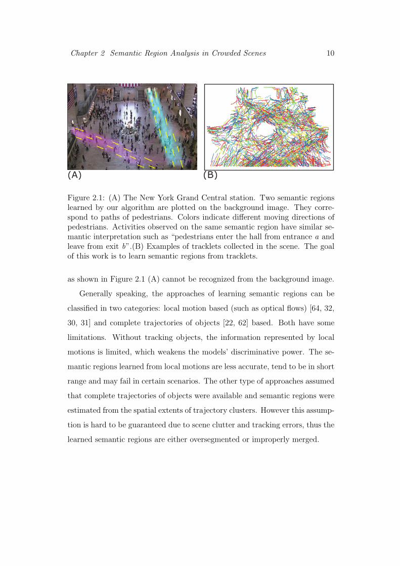
2.1 (A) The New York Grand Central station. Two semantic regions
learned by our algorithm are plotted on the background image.
They correspond to paths of pedestrians. Colors indicate dif-
ferent moving directions of pedestrians. Activities observed on
the same semantic region have similar semantic interpretation
such as “pedestrians enter the hall from entrance a and leave
from exit b”.(B) Examples of tracklets collected in the scene.
The goal of this work is to learn semantic regions from tracklets. 10
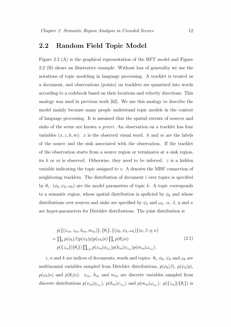
2.2 (A) Graphical representation of the RFT model. x is shadowed
since it is observed. h and m are half-shadowed because only
some of the observations have observed h andm. (B) Illustrative
example of our RFT model. Two kinds of MRF connect differ-
ent tracklets with observed and unobserved source/sink label
to enforce their spatial and temporal coherence. The semantic
region for the spanning tree is also plotted. . . . . . . . . . . . . 13
2.3 Algorithm of constructing the forest of randomly spanning trees. 15
2.4 Algorithm of obtaining the optimal spanning tree for online
tracklet. . . . . . . . . . . . . . . . . . . . . . . . . . . . . . . . 19
ix

2.5 (A) The histogram of tracklet lengths. (B) Detected source
and sink regions. (C) Statistics of sources and sinks of all the
tracklets. (D) The summary of observed sources and sinks of
the complete tracklets. . . . . . . . . . . . . . . . . . . . . . . . 20
2.6 Representative semantic regions learned by (A) our model (se-
mantic region indices are randomly assigned by learning pro-
cess), (B) OptHDP [64] and (C) TrajHDP [62]. The velocities
are quantized into four directions represented by four colors.
The two circles on every semantic region represent the learned
most probable source and sink. The boundaries of sources and
sinks in the scene are pre-detected and shown in Figure 2.5 (A).
(Better view in color version) . . . . . . . . . . . . . . . . . . . 23
2.7 Representative clusters of trajectories by (A)our model, (B)SC
[5] and (C)TrajHDP [62]. Colors of every trajectories are ran-
domly assigned. . . . . . . . . . . . . . . . . . . . . . . . . . . . 23
2.8 (A)(B) Transition probabilities from sources 2 and 6 to other
sinks. Only some major transition modes are shown. (C)(D)
Two online tracklets are extracted, and their optimal spanning
trees are obtained. The fitted curve for spanning trees predict
the compact paths of the individuals and their most possible
entry and exit locations are also estimated by our RFT model. . 25
x

3.1 A) The crowd of pedestrians walking in a train station. Pedestri-
ans have clear beliefs of the starting points and the destinations
in mind. These beliefs and scene structures (e.g. the border
of walls) influence their past behaviors (indicated as solid green
lines) as well as the future behaviors (indicated as dashed green
lines). The shared beliefs and dynamics of movements generate
several dominant collective dynamic patterns in the scene. B)
MDA learns the collective dynamic patterns of the crowd from
fragmented trajectories and simulates the collective behaviors
of the crowd. Yellow circles and red arrows represent the cur-
rent positions of the simulated pedestrians and their velocities,
along with their past trajectories in different colors. . . . . . . . 27
3.2 A) The behavior of a pedestrian in the crowd is influenced by
three key factors, the dynamics of movements, the belief of s-
tarting point and destination, and the timing of entering in the
scene. B) Graphical representation of the Mixture model of
Dynamic pedestrian-Agents. The shadowed variables are par-
tial observations of the hidden states due to frequent tracking
failures in crowded environment. . . . . . . . . . . . . . . . . . 29
3.3 A) Extracted trajectories and entry/exit regions indicated by
yellow ellipses. The colors of trajectories are randomly assigned.
B) Histogram of the lengths of trajectories. Most of them are
short and fragmented. . . . . . . . . . . . . . . . . . . . . . . . 38
xi

3.4 A) Illustration of eight representative dynamic pedestrian-agents
through sampling pedestrians from them. Green and red circles
indicate the distributions of initial/termination states for each
pedestrian-agent. Yellow circles indicate the current positions
of sampled pedestrians along their trajectories, and red arrows
indicate current velocities. The timings of pedestrians entering
the scene sampled from the Poisson process are shown below.
One impulse indicates a new pedestrian entering the scene driv-
en by the corresponding pedestrian-agent. B) Flow fields gen-
erated from dynamic pedestrian-agents. C) Flow fields learned
by LAB-FM [34]. . . . . . . . . . . . . . . . . . . . . . . . . . . 39
3.5 Four exemplar frames from the crowd behavior simulation. Sim-
ulated trajectories are colored according to the indices of their
dynamic pedestrian-agents. The middle plots the population of
pedestrians over time. . . . . . . . . . . . . . . . . . . . . . . . 40
3.6 A) The plot of all the simulated trajectories. Colors of trajecto-
ries are assigned according to pedestrian-agent indices. B) The
number of pedestrians entering the scene at different frames. C)
The capacity of the train station with λ = 0.5λ0, λ0, 1.5λ0, 2λ0
in simulation, where λ0 is the value learned from data. D) The
population density map of the train station computed from the
simulation. Color measures the relatively populated area. . . . . 41
3.7 Representative clusters of trajectories by A)MDAmodel, B)Spectral
Clustering [66] and C)HDP [62]. Colors of trajectories are ran-
domly assigned. . . . . . . . . . . . . . . . . . . . . . . . . . . . 42
3.8 A) An example of predicting behaviors with different methods.
B) The averaged prediction errors with different methods tested
on 30 trajectories. . . . . . . . . . . . . . . . . . . . . . . . . . 44
xii

4.1 Illustration of coherent neighbor invariance. The green dots
are the invariant K nearest neighbors of the central black dot
over time (here K = 7). The invariant neighbors have a higher
probability to be the dots moving coherently with the central
dot, since their local spatiotemporal relationships and velocity
correlations with the central dot are inclined to remain invariant
over time. The red and blue dots change their neighborship over
time (removed or added), so that they have a small probability
to move coherently with the central dot. . . . . . . . . . . . . . 47
4.2 A) Illustration of random dot kinematogram. Here the number
of coherent motion patternN = 1. The cyan arrows indicate the
moving directions of some noisy dots with incoherent motions.
The green arrows indicate the direction of coherent motion. B)
Averaged invariant neighbor ratios P with time interval d. C)
Averaged coherent invariant neighbor ratios W with time inter-
val d. All these measurements are computed and averaged for
coherent dots (referred as coherent), incoherent dots (referred
as incoherent) and all the dots (referred as mixed) respectively
for comparison. . . . . . . . . . . . . . . . . . . . . . . . . . . . 49
4.3 Histograms of gikt→d computed from all the invariant neighbors in
RDK, with d = 0, 1, 3, 5, 10 respectively. As d increases, gikt→d of
coherently moving dots and incoherently moving dots are well
separated. The bar near 1 is the histogram of gikt→d of coherently
moving dots, and the hump near 0 is the histogram of gikt→d of
incoherently moving dots. . . . . . . . . . . . . . . . . . . . . . 52
xiii
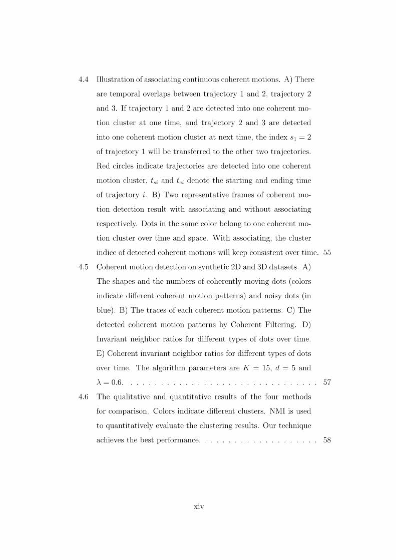
4.4 Illustration of associating continuous coherent motions. A) There
are temporal overlaps between trajectory 1 and 2, trajectory 2
and 3. If trajectory 1 and 2 are detected into one coherent mo-
tion cluster at one time, and trajectory 2 and 3 are detected
into one coherent motion cluster at next time, the index s1 = 2
of trajectory 1 will be transferred to the other two trajectories.
Red circles indicate trajectories are detected into one coherent
motion cluster, tsi and tei denote the starting and ending time
of trajectory i. B) Two representative frames of coherent mo-
tion detection result with associating and without associating
respectively. Dots in the same color belong to one coherent mo-
tion cluster over time and space. With associating, the cluster
indice of detected coherent motions will keep consistent over time. 55
4.5 Coherent motion detection on synthetic 2D and 3D datasets. A)
The shapes and the numbers of coherently moving dots (colors
indicate different coherent motion patterns) and noisy dots (in
blue). B) The traces of each coherent motion patterns. C) The
detected coherent motion patterns by Coherent Filtering. D)
Invariant neighbor ratios for different types of dots over time.
E) Coherent invariant neighbor ratios for different types of dots
over time. The algorithm parameters are K = 15, d = 5 and
λ = 0.6. . . . . . . . . . . . . . . . . . . . . . . . . . . . . . . . 57
4.6 The qualitative and quantitative results of the four methods
for comparison. Colors indicate different clusters. NMI is used
to quantitatively evaluate the clustering results. Our technique
achieves the best performance. . . . . . . . . . . . . . . . . . . . 58
xiv

4.7 A) Representative sequences from Hopkins155 database and the
segmentation results of Coherent Filtering. B) The first image is
one representative frame with groundtruth. There are 2 clusters,
one cluster is on the moving object, the other cluster is on the
static background objects, which results from moving camera.
The second image is the segmentation result of our method.
Since Coherent Filtering has no assumption on the number of
clusters, it tends to segment some dispersed background cluster
into several clusters of separated objects. Yellow + dots are the
detected noises. . . . . . . . . . . . . . . . . . . . . . . . . . . 58
4.8 A) NMI of different methods on the Hopkins155 Database, along
with the average computation time. Though Coherent Filter-
ing is not specifically designed for 3D motion segmentation, it
achieves comparative performance to other subspace segmenta-
tion methods with a better computational efficiency. B) NMI of
different methods as the function of the outlier percentage(from
0% to 400%). . . . . . . . . . . . . . . . . . . . . . . . . . . . . 59
xv
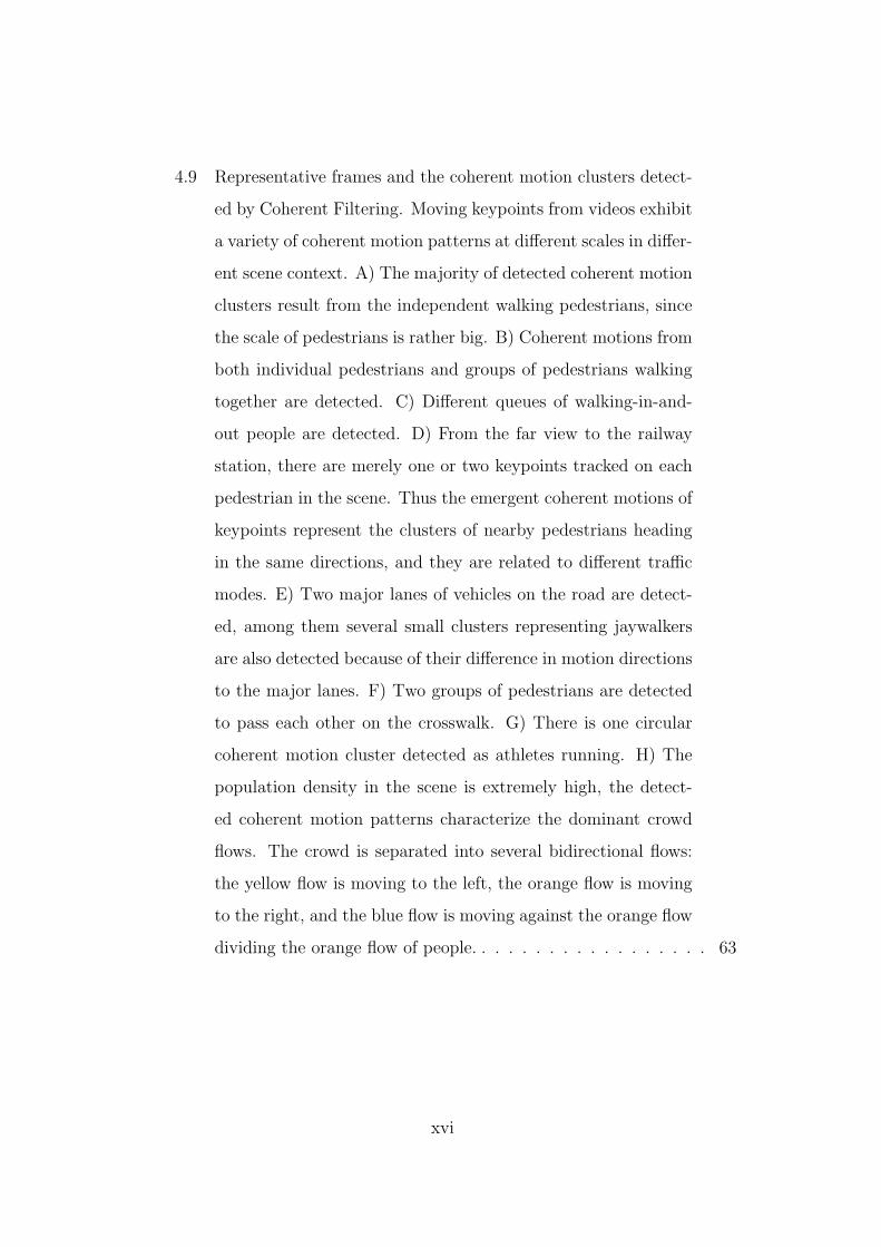
4.9 Representative frames and the coherent motion clusters detect-
ed by Coherent Filtering. Moving keypoints from videos exhibit
a variety of coherent motion patterns at different scales in differ-
ent scene context. A) The majority of detected coherent motion
clusters result from the independent walking pedestrians, since
the scale of pedestrians is rather big. B) Coherent motions from
both individual pedestrians and groups of pedestrians walking
together are detected. C) Different queues of walking-in-and-
out people are detected. D) From the far view to the railway
station, there are merely one or two keypoints tracked on each
pedestrian in the scene. Thus the emergent coherent motions of
keypoints represent the clusters of nearby pedestrians heading
in the same directions, and they are related to different traffic
modes. E) Two major lanes of vehicles on the road are detect-
ed, among them several small clusters representing jaywalkers
are also detected because of their difference in motion directions
to the major lanes. F) Two groups of pedestrians are detected
to pass each other on the crosswalk. G) There is one circular
coherent motion cluster detected as athletes running. H) The
population density in the scene is extremely high, the detect-
ed coherent motion patterns characterize the dominant crowd
flows. The crowd is separated into several bidirectional flows:
the yellow flow is moving to the left, the orange flow is moving
to the right, and the blue flow is moving against the orange flow
dividing the orange flow of people. . . . . . . . . . . . . . . . . . 63
xvi

4.10 A) The number of pedestrians detected at each key frame with
respect to Frame No., and Detection Rate(DR), False Alar-
m Rate(FAR), and counting error(CountError) for Coheren-
t Filter(CF), BayDet[9], and ALDENTE[48]. B) BayDet and
ALDENTE fail to detect the coherent motions when the crowd-
edness and the level of noise arise. . . . . . . . . . . . . . . . . . 64
4.11 A) Histograms of averaged velocity correlations of dots inA, and
the clustering results without thresholding, with d = 6, 10, 20 re-
spectively. And the plot of NMI under different d with thresh-
olding and without thresholding. B) Clustering results on the
2D synthetic data and the real data with K = 5 and K = 25
respectively. . . . . . . . . . . . . . . . . . . . . . . . . . . . . . 64
xvii

List of Tables
3.1 Algorithm for fitting a dynamic pedestrian-agent. . . . . . . . . 35
3.2 Algorithm for sampling a dynamic pedestrian-agent. . . . . . . . 36
4.1 Notations used in the paper. . . . . . . . . . . . . . . . . . . . . 48
4.2 Algorithm CoheFilterDet for detecting coherent motion pat-
terns. . . . . . . . . . . . . . . . . . . . . . . . . . . . . . . . . . 54
4.3 AlgorithmCoheFilterAssoci for associating continuous coher-
ent motion. . . . . . . . . . . . . . . . . . . . . . . . . . . . . . 56
xviii

Chapter 1
Introduction
1.1 Background of Crowd Behavior Analysis
Crowd behavior analysis is an interdisciplinary subject. Collective behaviors
of the crowd such as school fish, flocking birds and swarming ants have long
attracted the attentions of researchers over the few decades. Figure 1.1 shows
a variety of crowd behaviors in nature. Understanding the collective behaviors
of the crowd is one of the central problems in social science and natural science.
Social research works [29] have shown that when an individual is in the crowd,
he/she behaves differently to when he/she is alone. Other individuals in the
crowd and the external environment have a huge influence on his cognition
and action. In biology, the collective behaviors of organisms such as school
fish, flocking birds and swarming ants have long attracted the attention over
the few decades. Research works from both macroscopic level and microscopic
level are exploring the mechanism underlying the collective organization of
the individuals [12], the evolutionary origin of animal aggregation [44] and
the collective information processing in crowds [42]. Besides, some important
research topics such as self-organization, emergence, and phase transition have
also close relations to crowd behavior analysis, which attempt to find the
physical laws that govern the ways in which humans behave and organize
themselves [6].
1

Chapter 1 Introduction 2
Figure 1.1: The examples of crowd behaviors in human and animal popula-tions.
Research of crowd behavior analysis could lead to a lot of critical applica-
tions: 1) Video surveillance. Many places of security interests such as railway
station and shopping mall are very crowded, the conventional surveillance sys-
tem may not work well under such highly crowded environments. We can
leverage the results of crowd behavior analysis to better track and detect the
abnormal activities in these scenes [38]; 2) Crowd control. Based on crowd
behavior analysis, we could more efficiently recognize the traffic patterns, esti-
mate the traffic flow, and prevent any potential crowd disasters[16]; 3) Facility
optimization. Crowd behavior analysis provide guidelines for planning and de-
signing crowded areas. It helps improve the public facilities in these area, and
optimize their traffic capacity and make these areas more safe and convenient.
1.2 Previous Approaches and Related Works
1.2.1 Modeling Collective Motion
In recent years, there has been significant amount of work on learning the
motion patterns in crowded scenes due to growing interest in crowd behavior
analysis and crowd management. For example, Ali et al. [2] and Lin et al.

Chapter 1 Introduction 3
[34] computed the flow fields and segmented the patterns of crowd flows using
Lagrangian coherent structures or Lie algebra. Wang et al. [65] explored the
co-occurrence of moving pixels without tracking objects to learn the motion
patterns in crowded scenes. These approaches took the local location-velocity
pairs as input while ignoring the temporal order of observations in order to
be robust to tracking failures. The beliefs of pedestrians were not considered
either. Some approaches learned the motion patterns through clustering tra-
jectories [37, 63], and faced the challenge of fragmentation of trajectories in
crowded scenes. None of the above methods used agent-based models, which
could model the process of a pedestrian making decisions based on the current
states. It is difficult for them to simulate or predict collective crowd behaviors.
To analyze the interaction between pedestrians, the social force model, first
proposed by Helbing et al. [17, 15] for crowd simulation, was introduced to the
computer vision community recently and was applied to multi-target tracking
[45], abnormality detection [38], and interaction analysis [50]. The social force
model is also an agent-based model and assumes that pedestrians’ movements
for the next step are affected by their destinations, the states of their neighbors,
and the borders of buildings, walls, streets, and obstacles.
A number of pedestrian models for crowd simulation were proposed in com-
puter graphics. Continuum-based pedestrian models [24, 58] treated the crowd
motion as fluid with manually assigned parameters. Agent-based pedestrian
models [8] treated pedestrians as autonomous agents based on a set of defined
rules and known scene structures.
1.2.2 Semantic Region Analysis
Semantic regions correspond to different paths commonly taken by objects,
and activities observed in the same semantic region have similar semantic
interpretation. Semantic regions can be used for activity analysis in a single
Chapter 1 Introduction 4
camera view [64, 30, 31, 68, 62] or in multiple camera views [36, 32, 67] at
later stages. For example, in [64, 30, 31, 68] local motions were classified into
atomic activities if they were observed in certain semantic regions and the
global behaviors of video clips were modeled as distributions of over atomic
activities.
Wang et al. [64] used hierarchical Bayesian models to learn semantic re-
gions from the co-occurrence of optical flow features. It worked well for traffic
scenes where at different time different subsets of activities were observed.
However, our experiments show that it fails in a scene like Figure 2.1 (A),
where all types of activities happen together most of the time with significant
temporal overlaps. In this type of scenes, the co-occurrence information is
not discriminative enough. Some approaches [32, 30, 31] segmented semantic
regions by grouping neighboring cells with similar location or motion patterns.
Their segmentation results were not accurate and tended to be in short ranges.
Many trajectory clustering approaches first defined the pairwise distances
[26, 5] between trajectories, and then the computed distance matrices were in-
put to standard clustering algorithms [22]. Some other approaches [3, 69, 49]
of extracting features from trajectories for clustering were proposed in recent
years. Semantic regions were estimated from the spatial extents of trajectory
clusters. Reviews and comparisons of different trajectory clustering methods
can be found in [21, 39, 41]. It was difficult for those non-Bayesian approach-
es to include high-level semantic priors such as sources and sinks to improve
clustering. Wang et al. [62] proposed a Bayesian approach of simultaneous-
ly learning semantic regions and clustering trajectories using a topic model.
Tracklets were explored in previous works [13, 53, 35] mainly for the purpose
of connecting them into complete trajectories for better tracking or human
action recognition but not for learning semantic regions or clustering trajecto-
ries. Our approach does not require first obtaining complete trajectories from
tracklets.

Chapter 1 Introduction 5
In recent years, topic models borrowed from language processing were ex-
tended to capture spatial and temporal dependency to solve computer vision
problems. Hospedales et al. [18] combined topic models with HMM to analyze
the temporal behaviors of video clips in surveillance. A temporal order sensi-
tive topic model was proposed by Li et al. [32] to model activities in multiple
camera views from local motion features. Verbeek et al. [60] combined topic
models with MRF for object segmentation. Their model was relevant to ours.
In [60], MRF was used to model spatial dependency among words within the
same documents, while our model captures the spatial and temporal depen-
dency of words across different documents. Moreover, our model has extra
structures to incorporate sources and sinks.
1.2.3 Coherent Motion Detection
Coherent motion is a universal phenomenon in nature and widely exists in
many physical and biological systems. For example, tornadoes, storms, and
atmospheric circulation are all caused by the coherent movements of physical
particles in the atmosphere. The collective behaviors of organisms such as
swarming ants and schooling fishes have long captured the interests of social
and natural scientists [12, 42]. Detecting coherent motions and understanding
their underlying principles are related to many important scientific research
topics such as self-organization of biological systems [10] and collective intel-
ligence of the crowd [56]. There is also a wide range of practical application-
s. For example, in video surveillance, detecting coherent motion patterns of
pedestrian groups has important applications to object counting [48, 9], crowd
tracking [2], and crowd management [1]. Furthermore, clusters of coherent
motions provide a mid-level representation of crowd dynamics, and could be
used for high-level semantic analysis such as scene understanding and crowd
activity recognition [65, 18].

Chapter 1 Introduction 6
In recent years, there are some works proposed to detect coherent motion
patterns from clutters. For example, Rabaud et al. [48] and Brostow et al. [9]
proposed approaches to detect independent motions in order to count moving
objects. Lin et al. [34] used Lie algebra of affine transform to learn the
global motion patterns of crowds. Ali et al. [2] used floor fields from fluid
mechanics for the segmentation of crowd flows. Hu [20] clustered the single-
frame optical flows to learn the motion patterns. Meanwhile, the high-level
semantic analysis in crowded scenes focuses on modeling scene structures and
recognizing crowd behaviors. Wang et al. [65] and Hospedales et al. [18]
used hierarchial topic models to learn the models of semantic regions and the
models of crowd behaviors from the co-occurrence of optical flow features.
In 3D motion segmentation [59], under the assumption of affine transform
there are several subspace approaches proposed, such as Generalized Principal
Component Analysis (GPCA) [61] and RANSAC [59].
1.3 Our Works for Crowd Behavior Analysis
In the first part of this thesis work, a Random Field Topic (RFT) is proposed
for semantic region analysis from motions of objects in crowded scenes. Differ-
ent from existing approaches of learning semantic regions either from optical
flows or from complete trajectories, our model assumes that fragments of tra-
jectories (called tracklets) are observed in crowded scenes. It advances the
existing Latent Dirichlet Allocation topic model, by integrating the Markov
random fields (MRF) as prior to enforce the spatial and temporal coherence
between tracklets during the learning process. Two kinds of MRF, pairwise
MRF and the forest of randomly spanning trees, are defined. Another contri-
bution of this model is to include sources and sinks as high-level semantic prior,
which effectively improves the learning of semantic regions and the clustering
of tracklets. Experiments on a large scale data set, which includes 40, 000+

Chapter 1 Introduction 7
tracklets collected from the crowded New York Grand Central station, show
that our model outperforms state-of-the-art methods both on qualitative re-
sults of learning semantic regions and on quantitative results of clustering
tracklets. This work has been published in Proceedings of IEEE Conference
on Computer Vision and Pattern Recognition (CVPR) 2011.
In the second part of this thesis work, a new Mixture model of Dynamic
pedestrian-Agents (MDA) is proposed to learn the collective dynamics of
pedestrians from a large amount of observations without supervision. Obser-
vations are trajectories of feature points on pedestrians obtained by a KLT
tracker [57]. Because of frequent occlusions in crowded scenes, there are many
tracking failures, and most trajectories are highly fragmented with large por-
tions of missing observations. The movement of a pedestrian is driven by one
of the pedestrian-agents, which are modeled as linear dynamic systems with
initial and termination states (reflecting pedestrians’ beliefs of the starting
points and the destinations). Furthermore the timings of pedestrians entering
the scene with different dynamic patterns are modeled as Poisson processes.
Then, the collective dynamics of the whole crowd are modeled as a mixture
dynamic system. The effectiveness of MDA is demonstrated by three appli-
cations: simulating collective crowd behaviors, clustering trajectories into dif-
ferent collective behaviors, and predicting the behaviors of pedestrians. Both
qualitative and quantitative experimental evaluations are conducted on data
collected from the New York Grand Central Station. This work has been pub-
lished in Proceedings of IEEE Conference on Computer Vision and Pattern
Recognition (CVPR) 2012 as Oral.
In the third part of this thesis work, we propose and study a prior of coher-
ent motion called Coherent Neighbor Invariance, which characterizes the local
spatiotemporal relationships of individuals in coherent motion. Based on the
coherent neighbor invariance, a general technique of detecting coherent motion
patterns from noisy time-series data called Coherent Filtering is proposed. It

Chapter 1 Introduction 8
can be effectively applied to data with different global distributions at different
scales in various real-world problems, where the environments could be sparse
or extremely crowded with heavy noise. Experimental evaluation and com-
parison on synthetic and real data show the existence of coherence neighbor
invariance and the effectiveness of our coherent motion detection technique.
This work has been submitted to European Conference on Computer Vision
2012.
Chapter 2
Semantic Region Analysis in
Crowded Scenes
2.1 Introduction of Semantic Regions
In far-field video surveillance, it is of great interest to automatically segment
the scene into semantic regions and learn their models. These semantic regions
correspond to different paths commonly taken by objects, and activities ob-
served in the same semantic region have similar semantic interpretation. Some
examples are shown in Figure 2.1 (A). Semantic regions can be used for activ-
ity analysis in a single camera view [64, 30, 31, 68, 62] or in multiple camera
views [36, 32, 67] at later stages. For example, in [64, 30, 31, 68] local motions
were classified into atomic activities if they were observed in certain semantic
regions and the global behaviors of video clips were modeled as distributions of
over atomic activities. In [62], trajectories of objects were classified into differ-
ent activity categories according to the semantic regions they passed through.
In [36, 32], activities in multiple camera views were jointly modeled by explor-
ing the correlations of semantic regions in different camera views. Semantic
regions were also used to improve object detection, classification and tracking
[25, 14, 19]. Semantic regions are usually learned from motions of object in
order to better correlate with the activities of objects. Some semantic regions
9
Chapter 2 Semantic Region Analysis in Crowded Scenes 10
(A) (B)
Figure 2.1: (A) The New York Grand Central station. Two semantic regionslearned by our algorithm are plotted on the background image. They corre-spond to paths of pedestrians. Colors indicate different moving directions ofpedestrians. Activities observed on the same semantic region have similar se-mantic interpretation such as “pedestrians enter the hall from entrance a andleave from exit b”.(B) Examples of tracklets collected in the scene. The goalof this work is to learn semantic regions from tracklets.
as shown in Figure 2.1 (A) cannot be recognized from the background image.
Generally speaking, the approaches of learning semantic regions can be
classified in two categories: local motion based (such as optical flows) [64, 32,
30, 31] and complete trajectories of objects [22, 62] based. Both have some
limitations. Without tracking objects, the information represented by local
motions is limited, which weakens the models’ discriminative power. The se-
mantic regions learned from local motions are less accurate, tend to be in short
range and may fail in certain scenarios. The other type of approaches assumed
that complete trajectories of objects were available and semantic regions were
estimated from the spatial extents of trajectory clusters. However this assump-
tion is hard to be guaranteed due to scene clutter and tracking errors, thus the
learned semantic regions are either oversegmented or improperly merged.

Chapter 2 Semantic Region Analysis in Crowded Scenes 11
2.1.1 Our approach
We propose a new approach of learning semantic regions from tracklets, which
are a mid-level representation between the two extremes discussed above 1 .
A tracklet is a fragment of a trajectory and is obtained by a tracker within a
short period. Tracklets terminate when ambiguities caused by occlusions and
scene clutters arise. They are more conservative and less likely to drift than
long trajectories. In our approach, a KLT keypoint tracker [57] is used and
tracklets can be extracted even from very crowded scenes.
A Random Field Topic (RFT) model is proposed to learn semantic regions
from tracklets and to cluster tracklets. It advances the Latent Dirichlet Al-
location topic model (LDA) [7], by integrating MRF as prior to enforce the
spatial and temporal coherence between tracklets during the learning process.
Different from existing trajectory clustering approaches which assumed that
trajectories were independent given their cluster labels, our model defines two
kinds of MRF, pairwise MRF and the forest of randomly spanning trees, over
tracklets to model their spatial and temporal connections.
Our model also includes sources and sinks as high-level semantic prior. Al-
though sources and sinks were explored in existing works [37, 66] as important
scene structures, to the best of our knowledge they were not well explored to
improve the segmentation of semantic regions or the clustering of trajectories.
Our work shows that incorporating them in our Bayesian model effectively
improves both the learning of semantic regions and the clustering of tracklets.
Experiments on a large scale data set include more than 40, 000 tracklets
collected from the New York Grand Central station, which is a well known
crowded and busy scene, show that our model outperforms state-of-the-art
methods both on qualitative results of learning semantic regions and on quan-
titative results of clustering tracklets.
1Optical flows only track points between two frames. The other extreme is to trackobjects throughout their existence in the scene.
Chapter 2 Semantic Region Analysis in Crowded Scenes 12
2.2 Random Field Topic Model
Figure 2.2 (A) is the graphical representation of the RFT model and Figure
2.2 (B) shows an illustrative example. Without loss of generality we use the
notations of topic modeling in language processing. A tracklet is treated as
a document, and observations (points) on tracklets are quantized into words
according to a codebook based on their locations and velocity directions. This
analogy was used in previous work [62]. We use this analogy to describe the
model mainly because many people understand topic models in the context
of language processing. It is assumed that the spatial extents of sources and
sinks of the scene are known a priori. An observation on a tracklet has four
variables (x, z, h,m). x is the observed visual word. h and m are the labels
of the source and the sink associated with the observation. If the tracklet
of the observation starts from a source region or terminates at a sink region,
its h or m is observed. Otherwise, they need to be inferred. z is a hidden
variable indicating the topic assigned to x. Λ denotes the MRF connection of
neighboring tracklets. The distribution of document i over topics is specified
by θi. (ϕk, ψk, ωk) are the model parameters of topic k. A topic corresponds
to a semantic region, whose spatial distribution is speficied by ϕk and whose
distributions over sources and sinks are specified by ψk and ωk. α, β, η and κ
are hyper-parameters for Dirichlet distributions. The joint distribution is
p({(xin, zin, hin,min)}, {θi}, {(ϕk, ψk, ωk)}|α, β, η, κ)
=∏
k p(ϕk|β)p(ψk|η)p(ωk|κ)∏
i p(θi|α)
p({zin}|{θi})∏
i,n p(xin|ϕzin)p(hin|ψzin)p(min|ωzin).
(2.1)
i, n and k are indices of documents, words and topics. θi, ϕk, ψk and ωk are
multinomial variables sampled from Dirichlet distributions, p(ϕk|β), p(ψk|η),
p(ωk|κ) and p(θi|α). xin, hin and min are discrete variables sampled from
discrete distributions p(xin|ϕzin), p(hin|ψzin) and p(min|ωzin). p({zin}|{θi}) is
Chapter 2 Semantic Region Analysis in Crowded Scenes 13
pairwise
tree
SourceSink
MRF:
Tracklet:
x x
z z
φ
α
β
Λ
MRF
θi jθ
κ
ψ
η
ω
h m h m
N tracklets
K
Ni Nj
(B)
(A)
complete
only source
only sink
no source&sink
Figure 2.2: (A) Graphical representation of the RFT model. x is shadowedsince it is observed. h and m are half-shadowed because only some of theobservations have observed h and m. (B) Illustrative example of our RFTmodel. Two kinds of MRF connect different tracklets with observed and un-observed source/sink label to enforce their spatial and temporal coherence.The semantic region for the spanning tree is also plotted.
specified by MRF,
p(Z|θ) ∝ exp
∑i
logθi +∑j∈ε(i)
∑n1,n2
Λ(zin1 , zjn2)
. (2.2)
Z = {zij} and θ = {θi}. ε(i) is the set of tracklets which have dependency
with tracklet i and it is defined by the structure of MRF. Λ weights the de-
pendency between tracklets. Two types of MRF are defined in the following
sections.

Chapter 2 Semantic Region Analysis in Crowded Scenes 14
The intuition behind our model is interpreted as follows. According to
the property of topic models, words often co-occurring in the same documents
will be grouped into one topic. Therefore, if two locations are connected by
many tracklets, they tend to be grouped into the same semantic region. The
MRF term Λ encourages tracklets which are spatially and temporally close
to have similar distributions over semantic regions. Each semantic region has
its preferred source and sink. Our model encourages the tracklets to have the
same sources and sinks as their semantic regions. Therefore the learned spatial
distribution of a semantic region will connect its source and sink regions.
2.2.1 Pairwise MRF
For pairwise MRF, ε() is defined as pairwise neighborhood. A tracklet i s-
tarts at time tsi and ends at time tei . Its starting and ending points are at
locations (xsi , ysi ) and (xei , y
ei ) with velocities vs
i = (vsix, vsiy) and ve
i = (veix, veiy)
respectively. Tracklet j is the neighbor of i (j ∈ ε(i)), if it satisfies
I. tei < tsj < tei + T,
II. |xei − xsj|+ |yei − ysj | < S,
III.vei · vs
j
∥vei∥∥vs
j∥> C. (2.3)
I−III requires that tracklets i and j are temporally and spatially close and
have consistent moving directions. We try to find pairs of tracklets which
could be the same object and define them as neighbors in MRF. According to
I, tracklets with temporal overlap are not considered as neighbors, since it is
impossible for them to be the same objects. If these conditions are satisfied
and zin1 = zjn2 ,
Λ(zin1 , zjn2) = exp(vei · vs
j
∥vei∥∥vs
j∥− 1). (2.4)

Chapter 2 Semantic Region Analysis in Crowded Scenes 15
Algorithm Forest of Spanning Trees ConstructionINPUT: tracklet set IOUTPUT: Randomly spanning forest set T .01: for each tracklet i∈ I do02: initialize γ = ∅ /* γ is one spanning tree*/03: Seek-tree(i) /*Recursively search appropriate tree*/04: endfunction Seek-tree(tracklet m)/* Recursive search on neighboring tracklets defined
by Eq (2.3) */.01: γ ← m02: if tracklets in γ have at least one observed
source h and m do03: T ← γ /*add the tree to forest set*/04: break Seek-tree /*stop current search*/05: end06: for each j ∈ ε(m) do07: Seek-tree(tracklet j )08: end09: pop out γend
Figure 2.3: Algorithm of constructing the forest of randomly spanning trees.
Otherwise, Λ(zin1 , zjn2) = 0.
2.2.2 Forest of randomly spanning trees
The pairwise MRF only captures the connection between two neighboring
tracklets. To capture the higher-level dependencies among tracklets, the forest
of randomly spanning trees is constructed on top of the neighborhood defined
by the pairwise MRF. Sources and sinks are also integrated in the construction
process.
Sources and sinks refer to the regions where objects appear and disappear
in a scene. If an object is correctly tracked all the time, its trajectory has
a starting point observed in a source region and an ending point observed in

Chapter 2 Semantic Region Analysis in Crowded Scenes 16
a sink region. However, the sources and sinks of many tracklets extracted
from crowded scenes are unknown due to tracking error. Our model assumes
that the boundaries of source and sink regions of the scene are roughly known
either by manual input or automatic estimation [37] 2 . Experiments show
that accurate boundaries are not necessary. If the starting (or ending) point
of a tracklet falls in a source (or sink) region, its h (or m) is observed and is
the label of that region. Otherwise h (or m) is unobserved and needs to be
inferred.
The algorithm of constructing the forest of randomly spanning tree γ is
listed in Figure 2.3. A randomly spanning tree is composed of several tracklets
with pairwise connections, which are defined as the same in Eq (2.3). The
randomly spanning tree is constructed with the constraint that it starts with a
tracklet whose starting point has an observed source h and ends with a tracklet
whose ending point has an observed sink m. Then ε() in Eq (2.2) is defined
by the forest of randomly spanning tree γ, i.e. if tracklet i and j are on the
same randomly spanning tree, j ∈ γ(i).
2.2.3 Inference
We derive a collapsed Gibbs sampler to do inference. It integrates out {θ, ϕ, ψ, ω}
and samples {z, h,m} iteratively. The details of derivation are given in the
supplementary material. Here we just present the final result.
2In our approach, source and sink regions are estimated using the Gaussian mixturemodel [37]. Starting and ending points of tracklets caused by tracking failures are filteredconsidering the distributions of accumulated motion densities within their neighborhoods[66]. It is likely for a starting (ending) point to be in a source (sink) region, if the accumulatedmotion density quickly drops along the opposite (same) moving direction of its tracklet.After filtering, high-density Gaussian clusters correspond to sources and sinks. Low-densityGaussian clusters correspond to tracking failures. We skip the details since this is not thefocus of this paper.

Chapter 2 Semantic Region Analysis in Crowded Scenes 17
The posterior of zin given other variables is
p(zin = k|X,Z\in,H,M)
∝n(w)k,\in + β∑W
w=1(n(w)k,\in + β)
n(p)k,\in + η∑P
p=1(n(p)k,\in + η)
n(q)k,\in + κ∑Q
q=1(n(q)k,\in + κ)
n(k)i,\n + α∑K
k=1(n(k)i,\n + α)
exp
∑j∈γ(i)
∑n′
Λ(zin, zjn′)
. (2.5)
X = {xin},Z = {zin},H = {hin},M = {min}. Subscript \in denotes counts
over the whole data set excluding observation n on tracklet i. Denote that
xin = w, hin = p,min = q. n(w)k,\in denotes the count of observations with value
w and assigned to topic k. n(p)k,\in (n
(q)k,\in) denotes the count of observations
being associated with source p (sink q) and assigned to topic k. nki,\n denotes
the count of observations assigned to topic k on tracklet i. W is the codebook
size. P and Q are the numbers of sources and sinks.
The posteriors of hin and min given other variables are,
p(hin = p|X,Z,H\i,M) ∝n(p)k,\in + η∑P
p=1(n(p)k,\in + η)
, (2.6)
p(min = q|X,Z,H,M\in) ∝n(q)k,\in + κ∑Q
q=1(n(q)k,\in + κ)
. (2.7)
If hin and min are unobserved, they are sampled based on Eq (2.6) and
(2.7). Otherwise, they are fixed and not updated during Gibbs sampling.
After sampling converges, {θ, ψ, ω} could be estimated from any sample by

Chapter 2 Semantic Region Analysis in Crowded Scenes 18
ϕ(w)k =
n(w)k + β∑W
w=1(n(w)k + β)
, (2.8)
ψ(p)k =
n(p)k + η∑P
p=1(n(p)k + η)
, (2.9)
ω(q)k =
n(q)k + κ∑Q
q=1(n(q)k + κ)
. (2.10)
Once the RFT model is learnt, tracklets can be clustered based on semantic
regions they belong to. The topic label of a tracklet is obtained by majority
voting from its inferred z.
2.2.4 Online tracklet prediction
After semantic regions are learned, our model can online analyze the tracklets,
i.e. classifying them into semantic regions and predicting their sources and
sinks. It is unreliable to analyze an online tracklet alone using the models of
semantic regions, since when the tracklet is short it may fall into more than
one semantic region. Instead, we first obtain its optimal spanning tree from
the training set using the algorithm in Figure 2.4. It is assumed that a pedes-
trian’s behavior at one location is statistically correlated to the behaviors of
pedestrians in the training set at the same location. The algorithm first corre-
lates the online tracklet with the tracklets from the training set by generating
several spanning trees. The spanning tree with the minimum entropy on z is
chosen for the online tracklet to infer its topic label, source, and sink.
2.3 Experimental Results
Experiments are conducted on a 30 minutes long video sequence collected from
the New York’s Grand Central station. Figure 2.2 (B) shows a single frame of
this scene. The video is at the resolution of 480 × 720. 47, 866 tracklets are

Chapter 2 Semantic Region Analysis in Crowded Scenes 19
Algorithm Optimal Spanning Tree RankingINPUT: the online tracklet g, the learnt tracklet set IOUTPUT: Optimal spanning tree γ(g) and zγ for g.01: Exhaustively Seek neighbor grids ε of trajectory g
based on Constraint II and III in set I02: for each εi do03: γi ← Seek-tree(g) on εi04: Gibbs Sampling for zγi03: P ← γi / * P is the potential tree set * /04: end05: γ(g)=argmin
γ∈PH(Zγ)
/* H(Z) = −∑z
p(z)logp(z) is the information entropy,
computed over distribution of z for the spanning tree γi,to select the optimal spanning tree */.
Figure 2.4: Algorithm of obtaining the optimal spanning tree for online track-let.
extracted. The codebook of observations is designed as follows: the 480× 720
scene is divided into cells of size 10 × 10 and the velocities of keypoints are
quantized into four directions. Thus the size of the codebook is 48× 72× 4.
Figure 2.5 shows the summary of collected tracklets. (A) is the histogram
of tracklet lengths. Most of tracklet lengths are shorter than 100 frames. (B)
shows the detected sources and sinks regions indexed by 1 v 7. (C) shows the
percentages of four kinds of tracklets. Only a very small portion of tracklets
(3%) (labeled as “complete”) have both observed sources and sinks. 24%
tracklets (labeled as “only source”) only have observed sources. 17% tracklets
(labeled as “only sink”) only have observed sinks. For more than half of
tracklets (56%), neither sources nor sinks are observed. (D) summarizes the
observed sources and sinks of the complete tracklets. The vertical axis is the
source index, and horizontal axis is the sink index. It shows that most complete
tracklets are between the source/sink regions 5 and 6 since they are close in
space. Therefore, if only complete tracklets are used, most semantic regions

Chapter 2 Semantic Region Analysis in Crowded Scenes 20
1
2 3
4
5
7 6
(A) (B)
0
0.5
1
1.5
2
2.5
3x10⁴
complete
only source
only sink
no sink&source
23% 17%3% 57%
Source
Sink1 2 3 4 5 6 7
1234567
(D)
0 100 200 300 400 5000
0.5
1
1.5
2
2.5x 10
4
tracklet length / frames
(C)
num
ber
of tr
ackle
tsnum
ber
of tr
ackle
ts
Figure 2.5: (A) The histogram of tracklet lengths. (B) Detected source andsink regions. (C) Statistics of sources and sinks of all the tracklets. (D) Thesummary of observed sources and sinks of the complete tracklets.
cannot be well learned. Note that all tracklets come directly from the KLT
tracker, no preprocessing is involved in correcting the camera distortion for
tracklets.
Hyper-parameters α, β, η, κ are uniform Dirichlet distributions and are em-
pirically chosen as 1. Our results are not sensitive to these parameters. They
serve as priors of Dirichlet distributions to avoid singularity of the model, the
general discussion for the influence of the hyper-parameters on learning topic
model could be found in [7]. It takes around 2 hours for the Gibbs sampler to
converge on this data set, running on a computer with 3GHz core duo CPU in
Visual C++ implementation. The convergence is empirically determined by
the convergence of data likelihood, when the variation of data likelihood be-
comes trivial after hundreds of iteration of Gibbs sampling. The online tracklet
prediction takes 0.5 seconds per tracklet.

Chapter 2 Semantic Region Analysis in Crowded Scenes 21
2.3.1 Learning semantic regions
Our RFT model using the forest of randomly spanning trees learns 30 semantic
regions in this scene. In the learning process, around 23,000 randomly spanning
trees are constructed, and one tracklet may belong to more than one randomly
spanning tree. Figure 2.6 (A) visualizes some representative semantic regions.
According to the learned ψ and ω, the most probable source and sink for each
semantic region are also shown. The learned semantic regions represent the
primary visual flows and paths in the scene. They spatially expand in long
ranges and well capture the global structures of the scene. Meanwhile, most
paths are well separated and many structures are revealed at fine scales with
reasonably good accuracy. Most learned semantic regions only have one source
and one sink, except semantic region 19 which has two sources. Semantic re-
gion 14 also diverges. The results of these two regions need to be improved. It
is observed that sources and sinks, whose boundaries are defined beforehand,
only partially overlap with their semantic regions. One source or sink may
correspond to multiple semantic regions. This means that although the prior
provided by sources and sinks effectively guides the learning of semantic re-
gions, it does not add strong regularization on the exact shapes of semantic
regions. Therefore our model only needs the boundaries of sources and sinks
to be roughly defined.
For comparison, the results of optical flow based HDP (OptHDP) model
[64] and trajectory based Dual HDP (TrajHDP) [62] are shown in Figure 2.6
(B) and (C). Both methods are based on topic models. OptHDP learns the
semantic regions from the temporal co-occurrence of optical flow features and
it was reported to work well in traffic scenes [64]. It assumed that at different
time different subsets of activities happened. If two types of activities always
happen at the same time, they cannot be distinguished. In our scene, pedes-
trians move slowly in a large hall. For most of the time activities on different

Chapter 2 Semantic Region Analysis in Crowded Scenes 22
paths are simultaneously observed with large temporal overlaps. Temporal
co-occurrence information is not discriminative enough in this scenario. As
a result, different paths are incorrectly merged into one semantic region by
OptHDP as shown in Figure 2.6 (B). TrajHDP is related to our method. It
assumed that a significant portion of trajectories were complete and that if
two locations were on the same semantic region they were connected by many
trajectories. However, a large number of complete trajectories are unavailable
from this crowded scene. Without MRF and source-sink priors, TrajHDP can
only learn semantic regions expanded in short ranges. Some paths close in
space are incorrectly merged. For example, the two paths (21 and 15 in Fig-
ure 2.6 (A)) learned by our approach are close in the bottom-right region of
the scene. They are separated by our approach because they diverge toward
different sinks in the top region. However, since TrajHDP cannot well cap-
ture long-range distributions, they merge into one semantic region shown in
the fifth row of Figure 2.6 (C). Overall, the semantic regions learned by our
approach are more accurate and informative than OptHDP and TrajHDP.
2.3.2 Tracklet clustering based on semantic regions
Figure 2.7 (A) shows some representative clusters of tracklets obtained by our
model using the forest of randomly spanning trees as MRF prior. Even though
most tracklets are broken, some tracklets far away in space are also grouped
into one cluster because they have the same semantic interpretation. For
example, the first cluster shown in Figure 2.7 (A) contains tracklets related to
the activities of “pedestrians from source 2 walk toward sink 7”. It is not easy
to obtain such a cluster, because most tracklets in this cluster are not observed
either in source 2 or in sink 7. Figure 2.7 (B) and (C) show the representative
clusters obtained by Hausdorff distance-based Spectral Clustering (referred as
SC) [5] and TrajHDP [62]. They are all in short range spatially and it is hard

Chapter 2 Semantic Region Analysis in Crowded Scenes 23
(A) (B) (C)
10 21 15
11 18 1
9 6
16
14
19 27
direction
source
sink
interpretation
Figure 2.6: Representative semantic regions learned by (A) our model (seman-tic region indices are randomly assigned by learning process), (B) OptHDP[64] and (C) TrajHDP [62]. The velocities are quantized into four directionsrepresented by four colors. The two circles on every semantic region representthe learned most probable source and sink. The boundaries of sources andsinks in the scene are pre-detected and shown in Figure 2.5 (A). (Better viewin color version)
(A) (B) (C)
Figure 2.7: Representative clusters of trajectories by (A)our model, (B)SC [5]and (C)TrajHDP [62]. Colors of every trajectories are randomly assigned.

Chapter 2 Semantic Region Analysis in Crowded Scenes 24
to interpret their semantic meanings.
2.4 Discussion and Summary
In this chapter we proposed a new approach of learning semantic regions of
crowded scenes from tracklets, which are a mid-level representation between
local motions and complete trajectories of objects. It effectively uses the M-
RF prior to capture the spatial and temporal dependency between tracklets
and uses the source-sink prior to guide the learning of semantic regions. The
learned semantic regions well capture the global structures of the scenes in long
range with clear semantic interpretation. They are also able to separate differ-
ent paths at fine scales with good accuracy. Both qualitative and quantitative
experimental evaluations show that it outperforms state-of-the-art methods.
Our model also has other potential applications to be explored. For exam-
ple, after inferring the sources and sinks of tracklets, the transition probabilities
between sources and sinks can be estimated. It is of interest for crowd control
and flow prediction. Figure 2.8(A)(B) show the transition probabilities from
sources 2 and 6 to other sinks learned by our RFT model. Our model can also
predict the past and future behaviors of individuals whose existence is only
partially observed in a crowded scene. As shown in Figure 2.8(C)(D), two
individuals are being tracked, two online tracklets are generated. With the
algorithm in Figure 2.4 to obtain the optimal spanning tree, our model could
predict the most possible paths the individuals would take and estimate where
they came from and where they would go. To estimate individual behavior
in public crowded scenes is a critical feat for intelligent surveillance systems.
These applications will be explored in details in the future work.

Chapter 2 Semantic Region Analysis in Crowded Scenes 25
2
5
7 6
1
2 3
5
6
0.39 0.23
0.34
0.12
0.250.16
0.39
(A) (B)
spanning tree
fitted curve
online tracklet
spanning tree
fitted curve
online tracklet
1
3 2
6
(C)
(D)
7
1
3
4 4
Figure 2.8: (A)(B) Transition probabilities from sources 2 and 6 to other sinks.Only some major transition modes are shown. (C)(D) Two online trackletsare extracted, and their optimal spanning trees are obtained. The fitted curvefor spanning trees predict the compact paths of the individuals and their mostpossible entry and exit locations are also estimated by our RFT model.

Chapter 3
Learning Collective Crowd
Behaviors in Video
3.1 Understand Collective Crowd Behaviors
Automatically understanding the behaviors of pedestrians in crowd is of great
interest to video surveillance, and has drawn more and more attentions in
recent years [72]. It has important applications, such as event recognition [38],
traffic flow estimation [65], behavior prediction [4], and crowd simulation [58].
One of the underlying challenges of these problems is to model and learn the
collective dynamics of pedestrian behaviors in crowded scenes.
Crowd behavior analysis has been studied in social science with a long
history. French sociologist Le Bon (1841∼1931) described collective crowd
behaviors in his book The Crowd: A Study of the Popular Mind as, “the
crowd, an agglomeration of people, presents new characteristics very different
from those of the individuals composing it, the sentiments and ideas of all the
persons in the gathering take one and the same direction, and their conscious
personality vanishes. ” It leads to the motivation of this work: the crowd
has its intrinsic collective dynamics. Although individuals in crowd might not
acquaint with each other, their shared movements and destinations make them
coordinate collectively and follow the paths commonly taken by others [42].
26

Chapter 3 Learning Collective Crowd Behaviors in Video 27
A) B)
Figure 3.1: A) The crowd of pedestrians walking in a train station. Pedes-trians have clear beliefs of the starting points and the destinations in mind.These beliefs and scene structures (e.g. the border of walls) influence theirpast behaviors (indicated as solid green lines) as well as the future behaviors(indicated as dashed green lines). The shared beliefs and dynamics of move-ments generate several dominant collective dynamic patterns in the scene. B)MDA learns the collective dynamic patterns of the crowd from fragmentedtrajectories and simulates the collective behaviors of the crowd. Yellow circlesand red arrows represent the current positions of the simulated pedestriansand their velocities, along with their past trajectories in different colors.
An illustrative example is shown in Figure 3.1A.
A new Mixture model of Dynamic pedestrian-Agents (MDA) is proposed
to learn the collective dynamics of pedestrians from a large amount of obser-
vations without supervision. Observations are trajectories of feature points on
pedestrians obtained by a KLT tracker [57]. Because of frequent occlusions
in crowded scenes, there are many tracking failures, and most trajectories are
highly fragmented with large portions of missing observations. The movement
of a pedestrian is driven by one of the pedestrian-agents, which are modeled as
linear dynamic systems with initial and termination states (reflecting pedes-
trians’ beliefs of the starting points and the destinations). Furthermore the
timings of pedestrians entering the scene with different dynamic patterns are
modeled as Poisson processes. Then, the collective dynamics of the whole
crowd are modeled as a mixture dynamic system. The effectiveness of MDA
is demonstrated by three applications: simulating collective crowd behaviors,

Chapter 3 Learning Collective Crowd Behaviors in Video 28
clustering trajectories into different collective behaviors, and predicting the
behaviors of pedestrians. Both qualitative and quantitative experimental e-
valuations are conducted on data collected from the New York Grand Central
Station.
The novelty and contributions of this work are summarized as follows. 1)
Although there exist some approaches [18, 65, 34, 70] to learn motion patterns
in crowded scenes, they do not explicitly model the dynamics of pedestrians.
Many of them only took local location-velocity pairs as input, while discarding
the temporal order of trajectories, which is important for both classification
and simulation. Instead, MDA takes trajectories as input, and models the
temporal generative process of trajectories. Compared with those approaches,
it is much more natural for MDA to simulate collective crowd behaviors and
predict pedestrians’ future behaviors, once its parameters are learned from re-
al data. 2) Under MDA, pedestrians’ beliefs, which strongly regularize their
behaviors, are explicitly modeled and inferred from observations. In order to
be robust to tracking failures, the states of missing observations on trajec-
tories are modeled and inferred. Because of these two facts, MDA can well
infer the past behaviors and predict the future behaviors of pedestrians given
their trajectories only partially observed. They also lead to better accuracy of
recognizing the behaviors of pedestrians. 3) To the best of our knowledge, M-
DA is the first agent-based model to learn collective dynamics from the crowd
videos. Besides the collective dynamics, the behavior of a pedestrian is also
driven by the interactions with his/her neighbors. In the future work, it would
be much easier for MDA to integrate with the module of interactive dynamics
such as the social force model [17, 45], which is also an agent-based model.

Chapter 3 Learning Collective Crowd Behaviors in Video 29
Pedestrian
Timing
Scene
Dynamics Belief
A)
B)
Observations
States
Pedestrian agents
K
MM
...x1xs xa+1... xa+ τ
y1 y τ
... xT xe
...
D B
z
es
K
...x1xsxx xa+1xx ... xa+xx ττa+a+
y1 yτyy
... xTxx xe
...
z
Figure 3.2: A) The behavior of a pedestrian in the crowd is influenced by threekey factors, the dynamics of movements, the belief of starting point and des-tination, and the timing of entering in the scene. B) Graphical representationof the Mixture model of Dynamic pedestrian-Agents. The shadowed variablesare partial observations of the hidden states due to frequent tracking failuresin crowded environment.

Chapter 3 Learning Collective Crowd Behaviors in Video 30
3.2 Mixture Model of Dynamic Pedestrian-Agents
The crowd is an agglomeration of pedestrians. Although every pedestrian has
his own movement dynamics and belief of the starting point and the destina-
tion, some statistical dynamic patterns would appear when enough pedestri-
ans’ behaviors are observed over time, because pedestrians in a specific scene
share common movement dynamics and beliefs. These shared dynamic pat-
terns could be abstracted as different pedestrian-agents with various dynamics
and beliefs. In our model, dynamics and beliefs of pedestrians are modeled as
two key modules D and B in the agent system. Meanwhile, the timings of the
event that a pedestrian enters in the scene vary, because each pedestrian-agent
emerges at different frequency from the entry in the scene. We augment MDA
with another module, timing of emerging, for the dynamic pedestrian-agent.
Thus, the crowd in the scene is formulated as a mixture model of dynam-
ic pedestrian-agents as shown in Figure 3.2. In the following sections, each
module will be explained in details.
3.2.1 Modeling Pedestrian Dynamics
Trajectories extracted in the scene are time-series observations of pedestrian
dynamics. If we treat a pedestrian as a dynamic agent system which actively
senses the environment and makes decisions, the trajectory of the pedestrian
is a set of observations of the hidden dynamic states of this system. We model
the dynamics of a pedestrian-agent as a linear dynamic system defined by
xt = Axt−1 + ωt, (3.1)
yt = Cxt + εt. (3.2)
xt = [x1t , x2t , 1]
⊤ is the current state of the agent system and represents the
position of the agent in homogeneous coordinates. yt ∈ Rm is the observation
of xt. A ∈ R3×3 is the state transition matrix andC ∈ Rm×3 is the observation
Chapter 3 Learning Collective Crowd Behaviors in Video 31
matrix. ω is the system noise, and ε is the observation noise. Since the
observations of the agent system are its position, m is 3 and C is simplified
as a 3× 3 identity matrix. The conditional distributions of the state and the
observation are
p(xt|xt−1) = N (xt|Axt−1,Γ), (3.3)
p(yt|xt) = N (yt|xt,Σ), (3.4)
where N is the 3-dimensional multivariate Gaussian distribution, Γ and Σ are
covariance matrices. Σ is assumed to be a known diagonal matrix. We denote
D = (A,Γ) as the dynamics parameters to be learned for the agent system.
3.2.2 Modeling Pedestrian Beliefs
A pedestrian normally has a clear belief of the starting point and the desti-
nation when walking in a scene. This belief is a key factor driving the overall
behavior of the pedestrian, and it is also considered as the source and sink of
the scene [54, 70]. We model it as the initial state xs and the termination state
xe of the agent system. xs and xe are sampled from Gaussian distributions,
p(xs) = N (xs|µs,Φs),
p(xe) = N (xe|µe,Φe). (3.5)
µs and µe are the means of the initial states and termination states. Φs and
Φe are the corresponding covariance matrices. We denote B = (µs,Φs, µe,Φe)
as the belief parameters for the agent system.
For a trajectory k, the joint distribution of the system states and observa-
tions is
p(xk,yk,xks ,x
ke) = p(xk
s)p(xke)p(x
k1|xk
s)p(xke |xk
Tk)
Tk∏t=2
p(xkt |xk
t−1)
τk∏t=1
p(ykt |xk
ak+t), (3.6)

Chapter 3 Learning Collective Crowd Behaviors in Video 32
where xk = {xkt }
Tkt=1 and yk = {yk
t }τkt=1. yk is the partial observation of the
whole state xk. In crowded environments, the trajectories of objects are highly
fragmented due to the frequent occlusions among objects. Therefore, most
trajectories are only partially observed. We assume that trajectory k is only
observed from step ak + 1 to ak + τk. If ak = 0 and τk = Tk, the complete
trajectory is observed. The initial/termination states as well as the states of
missing observations have to be estimated from the model.
3.2.3 Mixture Model
There are numerous pedestrians with various dynamics and beliefs in a scene.
To model the diversity of pedestrian patterns, we extend the single agent sys-
tem described above to a mixture system of agents, withM possible dynamics
and beliefs (D1, B1), ..., (DM , BM). A hidden variable zk = 1, . . . ,M indi-
cates the mixture component, i.e. one pedestrian-agent system from which
a trajectory k is sampled. zk is sampled from a discrete prior distribution
parameterized by (π1, . . . , πM). The joint distribution is
p(xk,yk,xks ,x
ke , z
k)
=p(zk)p(xks |zk)p(xk
e |zk)p(xk1|xk
s , zk)p(xk
e |xkTk, zk)
Tk∏t=2
p(xkt |xk
t−1, zk)
τk∏t=1
p(ykt |xk
a+t, zk). (3.7)
3.2.4 Model Learning and Inference
Given the trajectories {yk}Kk=1, we would like to learn the model parameters
Θ = {(D1, B1), ..., (DM , BM)} by maximizing the likelihood of observations,
Θ∗ = argmaxΘ
K∑k=1
log p(yk; Θ). (3.8)
Since there are three kinds of hidden variables in the graphical model, 1) the
index zk of assigning a trajectory k to a mixture component, 2) the complete

Chapter 3 Learning Collective Crowd Behaviors in Video 33
sequence of states xk that produce the partial observation yk, and 3) the
number tek of steps with missing observations between xka+τ and the termination
state xke , and the number tsk of steps with missing observations between the
initial state xks and xa+1 (Tk = tek + tsk + τk, τk is the length of the fragmented
trajectory k). We apply the EM algorithm to estimate parameters. Each
iteration of EM consists of
E-step:Q = EX,T,Z|Y;Θ(log p(X,Y,T,Z; Θ)),
M-step:Θ∗ = argmaxΘQ(Θ; Θ).
where p(X,Y,T,Z; Θ) is the complete-data likelihood of the partial observa-
tions Y, complete hidden states X(including the initial states and termination
states), the numbers of steps with missing observations T, and hidden assign-
ment variables Z.
To initialize the estimation of the belief parameters, we first roughly draw
the boundaries of entry/exit regions in the scene as shown in Figure 3.3A. For
trajectories which start or end within these boundaries, their starting points
or ending points are used to estimate the belief parameters.
We summarize the derived EM algorithm on MDA as follows. In the E-step,
the posterior probabilities and the expectation of complete-data likelihood are,
Q =EX,T,Z|Y;Θ(log p(X,Y,T,Z; Θ))
=EZ,T|Y(EX|Y,Z(log p(X,Y,T,Z; Θ)))
=∑
k,m,g,h
γk(m, g, h)Exk|yk,zk=m,tsk=g,tek=h(p(xk,yk,xk
s ,xke , z
k))
where γk(m, g, h) is defined as
γk(m, g, h) =p(zk = m, tsk = g, tek = h | yk)
=πmp(y
k|zk = m, tsk = g, tek = h)∑Mm′=1
∑g′,h′ πm′p(yk|zk = m′, tsk = g′, tek = h′)
.
Chapter 3 Learning Collective Crowd Behaviors in Video 34
Here we assume the priors for p(ts) and p(te) are uniform distributions, and
they are independent with label zk.
In the M-step, the model parameters are updated as
Anewm =
∑k,g,h γk(m, g, h)
∑Tk
t=2 Pkt,t−1∑
k,g,h γk(m, g, h)∑Tk
t=2 Pkt−1,t−1
, (3.9)
Γnewm =
∑k,g,h γk(m, g, h)(
∑Tk
t=2 Pkt,t −Anew
m
∑Tk
t=2 Pkt,t−1)∑
k,g,h γk(m, g, h)(Tk + 1), (3.10)
µs,newm =
∑k,g,h γk(m, g, h)x
ks∑
k,g,h γk(m, g, h), (3.11)
Φs,newm =
∑k,g,h γk(m, g, h)(x
ks − µs
m)(xks − µs
m)⊤∑
k,g,h γk(m, g, h), (3.12)
µe,newm =
∑k,g,h γk(m, g, h)x
ke∑
k,g,h γk(m, g, h), (3.13)
Φe,newm =
∑k,g,h γk(m, g, h)(x
ke − µe
m)(xke − µe
m)⊤∑
k,g,h γk(m, g, h), (3.14)
πnewm =
∑k,g,h γk(m, g, h)∑M
m′=1
∑k,g,h γk(m
′, g, h). (3.15)
τk is the length of the trajectory k.
xk =Exk|yk,zk=m,tsk=g,tek=h(xk),
P kt,t =Exk|yk,zk=m,tsk=g,tek=h(xtx
⊤t ),
P kt,t−1 =Exk|yk,zk=m,tsk=g,tek=h(xtx
⊤t−1),
and γk(m, g, h) are all computed efficiently by modified Kalman smooth-
ing filter [43, 52], which can recursively estimate the hidden states given
the partial observations. Note that γk(m, g, h) has three discrete variables,
it is time consuming to enumerate and compute all their possible combi-
nations. However, for most (g, h), γk(m, g, h) are approximately to 0. We

Chapter 3 Learning Collective Crowd Behaviors in Video 35
Table 3.1: Algorithm for fitting a dynamic pedestrian-agent.
INPUT: trajectory k from any tracker.OUTPUT: the optimal fitted z∗.01: for m = 1 :M do02: compute γ(zk = m) =
∑g,h γk(m, g, h)
03: end for04:z∗ = argmaxm γ(z
k = m)05:compute the future state or past state with Az∗ .predict its belief with Bz∗ .
first get the most plausible h = argmint ∥ µem − At
mykτ ∥, g = argmint ∥
µsm −A−t
m yk1 ∥ by gradient descent. Then we limit the plausible range of tsk as
[g −∆, g −∆+ 1, ..., g, ..., g +∆ − 1, g +∆], and the plausible range of tek as
[h−∆, h−∆+1, ..., h, ..., h+∆−1, h+∆], where ∆ is an integer and empirically
determined. When it is out of the plausible range, γk(m, g, h) is approximated
as 0. For each combination, the total step of all states Tk = τk + tek + tsk.
3.2.5 Algorithms for Model Fitting and Sampling
After the parameters of MDA are learned, given the fragmented trajectory
of a pedestrian in the scene, our model can fit it to the optimal pedestrian-
agent and predict the pedestrian’s past and future paths, as well as the belief
of the starting point and the destination. Meanwhile, by sampling from the
pedestrian-agent model we can generate the trajectories characterized by this
pedestrian-agent. These two important properties of MDA model will be used
in the following experiments. The algorithms of fitting a dynamic pedestrian-
agent and sampling trajectories from it are listed in Table 3.1 and 3.2.

Chapter 3 Learning Collective Crowd Behaviors in Video 36
Table 3.2: Algorithm for sampling a dynamic pedestrian-agent.
INPUT: time length T , pedestrian-agent mOUTPUT: simulated trajectories.01:sample temporal order δ1∼T from PoissonP (λm)02:for ω = 1 : T03: if δω == 104: sample xs from pm(xs)05: τ = argmint ∥ µe
m −Atmxs ∥.
06: generate trajectory {yt}τt=1 by sequentiallysampling pm(xt|xt−1) and pm(yt|xt).
07: end if08:end for
3.3 Modeling Pedestrian Timing of Emerging
To fully capture the dynamics of pedestrians in the scene, we model pedestrian
timings of emerging, i.e. the frequency of new pedestrians entering in the scene
over time, and integrate this module into MDA.
Considering the event that a pedestrian emerges in an entry region, we as-
sume the timing of that event follows a homogeneous Poisson process PoissonP (λ),
whose underlying distribution is a Poisson distribution
p(n;λ) =λne−λ
n!, (3.16)
where n is the number of events that occur during an unit time interval. λ is
the rate parameter of the Poisson process, and indicates the expected number
of events that occur per unit time interval.
After {(D1, B1), ..., (DM , BM)} being learned by the EM algorithm, every
trajectory k has the most likely zk, and its emerging time can also be esti-
mated. Thus we can count the number of emerging pedestrians in each time
interval (here we use 5 seconds), and estimate the rate parameter λm for each

Chapter 3 Learning Collective Crowd Behaviors in Video 37
pedestrian-agent m by maximum likelihood estimation,
λm =1
L
L∑i=1
nmi , (3.17)
where L is the number of time intervals over the whole video sequence, and nmi
is the number of emerging pedestrians generated from the dynamic pedestrian-
agent m in time interval i.
3.4 Experiments and Applications
Experiments are conducted on a 15 minute long video sequence collected from
the New York Grand Central Station. The video is 24fps with a resolution
of 480×7201 . A KLT keypoint tracker [57] is used to extract trajectories.
Tracking terminates when ambiguities caused by occlusions and scene clutters
arise, and new tracks will be initialized later. After filtering some short or
stationary trajectories, around 20,000 trajectories are extracted and shown in
Figure 3.3A. Figure 3.3B plots the histogram of the lengths of trajectories. It
shows that most trajectories are highly fragmented, and exist only for short
periods.
3.4.1 Model Learning
To initialize the belief parameters of MDA, we first roughly label 8 entry/exit
regions with ellipses indexed by 1∼8 in Figure 3.3A. The parameters will be
updated at the learning stage. Trajectories which start/end within these re-
gions have observed initial/termination states. Their starting/ending points
are used to initialize the estimation of parameters (µsm,Φ
sm, µ
em,Φ
em). After
initialization, all the parameters of MDA are automatically learned from the
observations. It takes around one hour for the EM algorithm to converge, run-
ning on a computer with 3GHz Core Quad CPU and 4GB RAM with Matlab
1Data is available at http://www.ee.cuhk.edu.hk/∼xgwang/grandcentral.html

Chapter 3 Learning Collective Crowd Behaviors in Video 38
B)A)0 200 400 600 800
0
2000
4000
6000
8000
num
ber
of tr
aje
cto
ries
length/frames
1
2 3 4
5
6
78
Figure 3.3: A) Extracted trajectories and entry/exit regions indicated by yel-low ellipses. The colors of trajectories are randomly assigned. B) Histogramof the lengths of trajectories. Most of them are short and fragmented.
implementation. Totally M = 20 agent components are learned. In this work,
M is chosen empirically, but it also could be estimated with Dirichlet process
[65].
Figure 3.4A illustrates eight representative dynamic pedestrian-agents. Tra-
jectories are sampled from each pedestrian-agent using the algorithm in Table
3.2. Results show that the learned dynamic pedestrian-agents have different
dynamics, beliefs and timings of emerging, and they characterize various col-
lective behaviors. By densely sampling, MDA also can estimate the velocity
flow field for each pedestrian agent as shown in Figure 3.4B. For comparison,
the representative flow fields learned by LAB-FM [34], which tried to learn
motion patterns using Lie algebra, are shown in Figure 3.4C. MDA perform-
s better in terms of capturing long-range collective behaviors and separating
different collective behaviors. For example, some flow fields learned by LAB-
FM are locally distributed, without covering the complete paths. The upper
parts of the first two flow fields in Figure 3.4B, which represent two different
collective behaviors, are merged by LAB-FM as shown in the first flow field in
Figure 3.4C. This is due to the facts that 1) MDA better models the shared
beliefs of pedestrians and states of missing observations, and takes the whole

Chapter 3 Learning Collective Crowd Behaviors in Video 39
0 500 1000 1500 2000 2500 3000
0
1
Frame No.534: Current pedestrian number=18
0 500 1000 1500 2000 2500 3000
0
1
Frame No.3521: Current pedestrian number=25
0 500 1000 1500 2000 2500 3000
0
1
Frame No.1566: Current Pedestrian number=11
0 500 1000 1500 2000 2500 3000
0
1
Frame No.2582: Current Pedestrian number=23
0 500 1000 1500 2000 2500 3000
0
1
Frame No.729: Current pedestrian number=6 Frame No.378: Current pedestrian number=11
500 1000 1500 2000 2500 30000
1
0
0 500 1000 1500 2000 2500 3000
0
1
Frame No.1291: Current pedestrian number=20
0 500 1000 1500 2000 2500 3000
0
1
Frame No.508: Current pedestrian number=15
A) B) C)
Figure 3.4: A) Illustration of eight representative dynamic pedestrian-agentsthrough sampling pedestrians from them. Green and red circles indicate thedistributions of initial/termination states for each pedestrian-agent. Yellowcircles indicate the current positions of sampled pedestrians along their trajec-tories, and red arrows indicate current velocities. The timings of pedestriansentering the scene sampled from the Poisson process are shown below. One im-pulse indicates a new pedestrian entering the scene driven by the correspondingpedestrian-agent. B) Flow fields generated from dynamic pedestrian-agents.C) Flow fields learned by LAB-FM [34].
trajectories instead of local position-velocity pairs as input, and also that 2)
LAB-FM assumes that the spatial distributions of the flow fields are Gaussian
(indicated by cyan ellipses).
3.4.2 Collective Crowd Behavior Simulation
Compared with other approaches [18, 65, 70] of modeling global motion pat-
terns in crowded scenes, one of the distinctive features of MDA is to sim-
ulate collective crowd behaviors once it is learned from observations. Ac-
cording to the superposition property of Poisson process [27], the timings of
overall pedestrians entering the scene also follow a Poisson distribution with
λ =∑M
m=1 λm. To simulate a trajectory, its pedestrian-agent index is first sam-
pled from the discrete distribution (π1, ..., πM) then its trajectory is sampled
from the pedestrian-agent using the algorithm in Table 3.2.
Figure 3.5 shows four exemplar frames of the simulated crowd behaviors. At

Chapter 3 Learning Collective Crowd Behaviors in Video 40
0 500 1000 1500 2000 2500 3000 3500 4000 45000
100
200
300
Frame No.620: Current pedestrian number=128
Frame No.3256: Current pedestrian number=211
Frame No.232: Current pedestrian number=49
Frame No.
Ped. No.
Frame No. 1752: Current pedestrian number=221
Figure 3.5: Four exemplar frames from the crowd behavior simulation. Sim-ulated trajectories are colored according to the indices of their dynamicpedestrian-agents. The middle plots the population of pedestrians over time.
the first frame pedestrians begin to enter the empty scene. After 1500 frames
the crowd reaches the equilibrium population with around 200 pedestrians.
Our model well learns the dynamics of the crowd, and the simulated pedestrian
behaviors are similar to those observed in the real data.
Figure 3.6A plots all the simulated trajectories over 4500 frames. Figure
3.6B shows the timings of emerging of the crowd, i.e. the numbers of new
pedestrians entering the scene over time. The crowd simulation with MDA
can provide some valuable information about the dynamics of the crowd in the
scene. For example, in Figure 3.6C, we investigate the relationship between the

Chapter 3 Learning Collective Crowd Behaviors in Video 41
A)
D)0 1000 2000 3000 4000 5000 6000 7000
0
100
200
300
400
500
600
λ λ λ λ0.5 1.5 2
Frame.No.
Pe
de
str
ian
No
.
0 1000 2000 3000 4000 45000
1
2
3
4
5
B)
C)
Frame.No.
Em
erg
e N
o.
0
0.2
0.4
0.6
0.8
1
00 0 0
Figure 3.6: A) The plot of all the simulated trajectories. Colors of trajectoriesare assigned according to pedestrian-agent indices. B) The number of pedestri-ans entering the scene at different frames. C) The capacity of the train stationwith λ = 0.5λ0, λ0, 1.5λ0, 2λ0 in simulation, where λ0 is the value learned fromdata. D) The population density map of the train station computed from thesimulation. Color measures the relatively populated area.
different rate parameter λ and the capacity of the train station, where pedes-
trians begin and stop to enter the scene at the Frame 1 and 6000 respectively.
As pedestrians keep entering the scene with a constant birth rate, the scene
will reach its capacity, which is the equilibrium state of the system. When
λ = λ0, which is learned from data, the system reaches its equilibrium state
after 1500 frames with around 200 pedestrians in the scene. So the capacity
of the scene could be measured as 200. And the equilibrium state will change
with different birth rates as shown in Figure 3.6C. In Figure 3.6D we compute
the averaged population density map when λ = λ0, the populated areas of
the scene are detected. These areas should deserve high attention of security
since accidents would most likely happen there when panic or abnormal event

Chapter 3 Learning Collective Crowd Behaviors in Video 42
A) B) C)
Figure 3.7: Representative clusters of trajectories by A)MDA model,B)Spectral Clustering [66] and C)HDP [62]. Colors of trajectories are ran-domly assigned.
strikes. These types of information are very useful for the crowd management
and the public facility optimization.
3.4.3 Collective Behavior Classification
Once MDA is learned from observations without supervision, it can be used
to cluster the trajectories of pedestrians into different collective dynamics. We
simply take the inferred index zk of every trajectory as its cluster index. A
lot of works have been done on trajectory clustering in video surveillance.
This problem is especially challenging in crowded scenes because trajectories
are highly fragmented with many missing observations. Generally speaking,
existing approaches are in two categories: distance-based [66, 23] and model-
based [63]. We choose one representative approach from each category for
comparison: Hausdorff distance-based spectral clustering [66] and hierarchical
Dirichlet processes (HDP) [63].
Figure 3.7A shows some representative clusters of trajectories obtained by
MDA. Even though most trajectories are fragmented and are far away from
each other in space, they are still well grouped into one cluster because they
share the same collective dynamics. For example, the first cluster in Figure
3.7A explains the collective behavior of “pedestrians walking from entry 7 to

Chapter 3 Learning Collective Crowd Behaviors in Video 43
exit 2”. Figure 3.7B and Figure 3.7C show the representative clusters obtained
by spectral clustering [66] and HDP [63]. They are all in short spatial range
and it is hard to interpret their semantic meanings, because they cannot well
handle the fragmentation of trajectories.
3.4.4 Behavior Prediction
MDA can predict pedestrians’ behaviors given that their trajectories are only
partially observed. We manually label 30 trajectories of pedestrians as ground-
truth. For each ground-truth trajectory, we use the observations of the first
20 frames to estimate its pedestrian-agent index z with the algorithm in Table
3.1. Then, the model of the selected pedestrian-agent is used to recursively
generate the following states as the predicted future trajectory. The perfor-
mance is measured by the averaged prediction error, i.e. deviation between
the predicted trajectories and the ground-truth trajectories.
Two baseline methods are used for comparison. In the first comparison
method(referred as ConVelocity), a constant velocity which is estimated as
the averaged velocity of the past observations, is used to predict the future
positions. In the second comparison method LAB-FM [34], the learned flow
field which best fit the first 20 frame observations, is used to predict future
positions. The results in Figure 3.8 show that MDA has better prediction
performance.
3.5 Discussion and Summary
In this chapter, we propose a Mixture model of Dynamic Pedestrian-Agents to
learn the collective dynamics from video sequences in crowded scenes. Through
modeling the beliefs of pedestrians and the missing states of observations, it
can be well learned from highly fragmented trajectories caused by frequent
tracking failures. It can not only classify collective behaviors, but also simulate
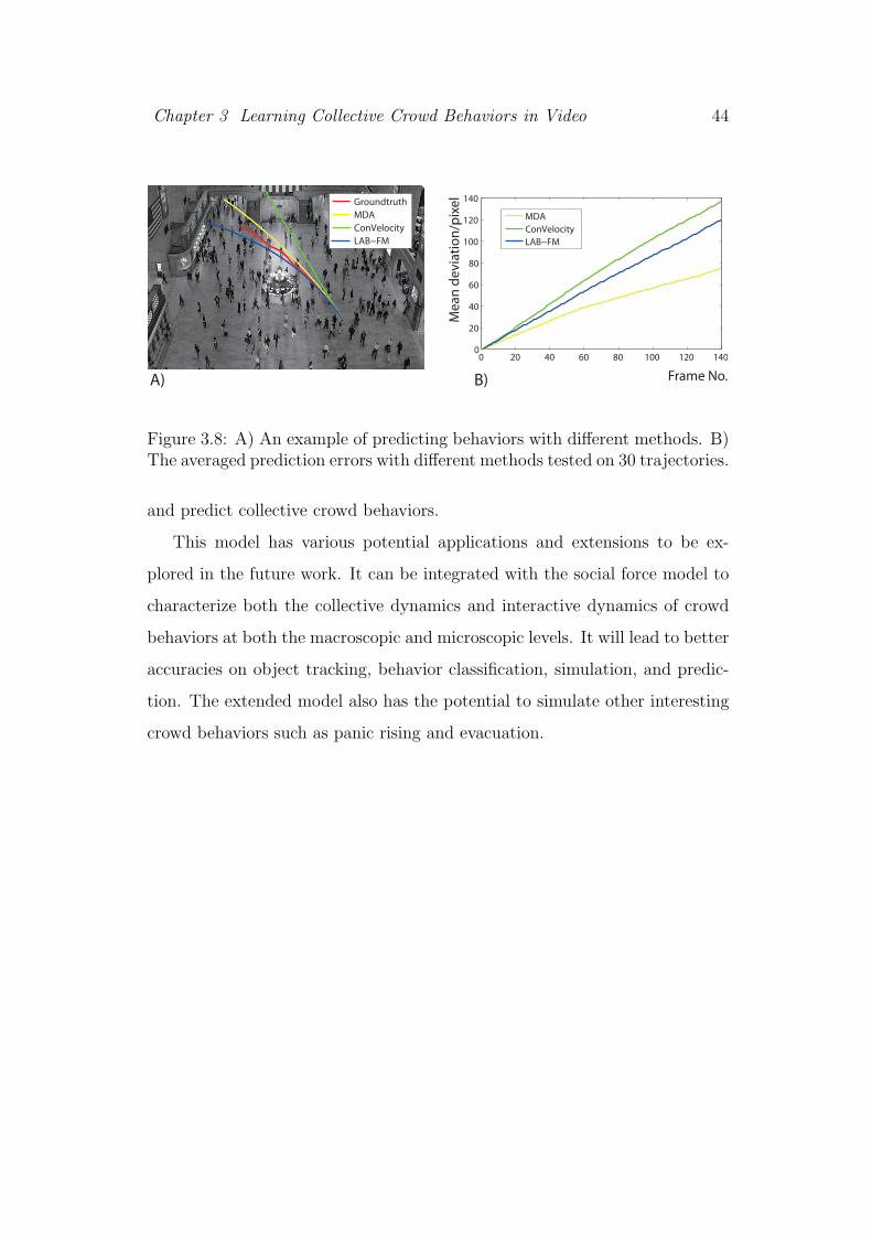
Chapter 3 Learning Collective Crowd Behaviors in Video 44
Groundtruth
MDA
ConVelocity
LAB−FM
0 20 40 60 80 100 120 1400
20
40
60
80
100
120
140
MDA
ConVelocity
LAB−FM
Frame No.
Me
an
de
via
tio
n/p
ixe
l
A) B)
Figure 3.8: A) An example of predicting behaviors with different methods. B)The averaged prediction errors with different methods tested on 30 trajectories.
and predict collective crowd behaviors.
This model has various potential applications and extensions to be ex-
plored in the future work. It can be integrated with the social force model to
characterize both the collective dynamics and interactive dynamics of crowd
behaviors at both the macroscopic and microscopic levels. It will lead to better
accuracies on object tracking, behavior classification, simulation, and predic-
tion. The extended model also has the potential to simulate other interesting
crowd behaviors such as panic rising and evacuation.

Chapter 4
Detecting Coherent Motions
from Clutters
4.1 Coherent Motions in Nature
Coherent motion is a universal phenomenon in nature and widely exists in
many physical and biological systems. For example, tornadoes, storms, and
atmospheric circulation are all caused by the coherent movements of physical
particles in the atmosphere. The collective behaviors of organisms such as
swarming ants and schooling fishes have long captured the interests of social
and natural scientists [12, 42].
Generally speaking, coherent motion detection can be formulated as finding
clusters of particles with coherent motion patterns from time-series data and
removing background noise as outliers. Under different scene context, the
detected coherent motions may be interpreted as different semantic behaviors.
As shown in Figure 4.9, moving keypoints tracked in the scenes exhibit a wide
variety of coherent motion patterns, corresponding to individual and group
movements, traffic mode, crowd flow etc. These examples show that detecting
coherent motions from noisy observations is of great importance to activity
analysis and scene understanding.
The goal of this work is to explore the common prior in the dynamics of
45
Chapter 4 Detecting Coherent Motions from Clutters 46
coherent motions and to leverage them for coherent motion detection. We
propose a prior called Coherent Neighbor Invariance, which exists in the local
neighborhoods of individuals in coherent motions, and show that it well distin-
guishes coherent and incoherent motions. Then we develop a general coherent
motion detection technique called Coherent Filtering based on such a prior.
It solves the problem through dynamic clustering and groups samples whose
states change over time in an online mode.
4.2 A Prior of Coherent Motion
Although coherent motions are the macroscopic observations of collective move-
ments of individuals, recent studies [42, 47] show that it actually can be char-
acterized by the interactions among individuals within local neighborhoods.
Inspired by these observations and results, we propose a prior underlying the
dynamics of coherent motion as Coherent Neighbor Invariance. There are two
key properties of Coherent Neighbor Invariance, which distinguish coherent
motions from random motions:
• Invariance of spatiotemporal relationships: the neighborship of individ-
uals with coherent motions is inclined to remain invariant over time.
• Invariance of velocity correlations: the velocity correlations of neighbor-
ing individuals with coherent motions remain high when being averaged
over time.
On the contrary, incoherently moving individuals do not have such proper-
ties because of the mutual independence of their movements. Coherent neigh-
bor invariance exists in the dynamics of K nearest neighbors of individuals
for consecutive time. It characterizes the local self-organization of coherent
motions, and explains the generation of global coherent motion patterns from

Chapter 4 Detecting Coherent Motions from Clutters 47
time t time t+1 time t+2
center
invariant neighbor
removed
added
unrelated
Figure 4.1: Illustration of coherent neighbor invariance. The green dots arethe invariant K nearest neighbors of the central black dot over time (here K =7). The invariant neighbors have a higher probability to be the dots movingcoherently with the central dot, since their local spatiotemporal relationshipsand velocity correlations with the central dot are inclined to remain invariantover time. The red and blue dots change their neighborship over time (removedor added), so that they have a small probability to move coherently with thecentral dot.
local coordinations of individuals. An illustration of the prior is shown in
Figure 4.1.
To quantitatively analyze this prior, we first define two measurements of
Coherent Neighbor Invariance: the coherent neighbor invariance of spatiotem-
poral relationships (in Section 4.2.2), and the coherent neighbor invariance of
velocity correlations (in Section 4.2.3). From the following experiments, we
show that this prior not only helps reveal the mechanism of coherent motion-
s, but also can be effectively leveraged to separate various coherent motion
patterns from background noise using a technique called Coherent Filtering.
4.2.1 Random Dot Kinematogram
We take Random Dot Kinematogram (RDK) as an example to analyze the
coherent neighbor invariance, because it is easy to understand and can be well
generalized. RDK is a classic psychophysical stimulus, and is often used for
investigating coherent motion perception of visual systems [28]. The stimulus

Chapter 4 Detecting Coherent Motions from Clutters 48
| · | The cardinality of a set.∩ The intersection of two sets.F F = {F1, ...,FN}. The set of coherent dots.B The set of incoherent dots.N i
t N it = {i1t , ..., iKt }. The set of the K-NNs of dot i at time t.
Mit→d Mi
t→d = N it ∩N i
t+1 ∩ ... ∩N it+d.
The dth order invariant neighbor set of i.Cit→d Ci
t→d = Mit→d ∩ F . The coherent invariant neighbor set of i
gikt→d Averaged velocity correlation between i and ik from t to t+ d.A A = ∪iMi
t→d.The set of all dth order invariant neighbor dots.
R R = {(i, ik)|gikt→d > λ, ik ∈ A}. The set of pairwise connections.
S S = {si|i ∈ I}. The set of the cluster index si for each dot i.
Table 4.1: Notations used in the paper.
consists of a completely random array of thousands of tiny dots that move
either coherently or randomly. An illustration is shown in Figure 4.2A. In-
coherently moving dots are randomly placed over the whole scene and serve
as background noise. In the central rectangular area, a group of coherently
moving dots are also randomly placed. The proportion of coherent dots to
all the dots in the rectangular area (mixing of coherent dots and incoherent
dots) is called the coherence level. In psychophysical study, human subjects
are required to identify coherent motions of dots from the background noise.
The coherence level determines the difficulty level of the identification task.
Formally, we denote I as the set of all the dots (mixed dots) in the central
rectangular area, F as the set of coherent dots, and B as the set of incoherent
dots. There could be N different coherent motion patterns which divide F
into subsets {F1, ...,FN}. Thus the problem of detecting coherent motions
from noisy observations of dot movements is formulated as estimating the
separation I = {F ,B}, and the sub-separation F = {F1, ...,FN}. In Sections
4.2.2 and 4.2.3, we will analyze two coherent neighbor invariance measurements
and study their dynamic behaviors. Table 4.1 shows the notations used in the
paper.

Chapter 4 Detecting Coherent Motions from Clutters 49
Coherent Invariant Neighbor RatioInvariant Neighbor Ratio
A) B) C)time interval d
Pw
time interval dCoherence Level=0.30 5 10 15
0
0.2
0.4
0.6
0.8
1
mixed
cohrent
incoherent
0 5 10 150
0.2
0.4
0.6
0.8
1
mixed
coherent
incoherent
Figure 4.2: A) Illustration of random dot kinematogram. Here the number ofcoherent motion pattern N = 1. The cyan arrows indicate the moving direc-tions of some noisy dots with incoherent motions. The green arrows indicatethe direction of coherent motion. B) Averaged invariant neighbor ratios P withtime interval d. C) Averaged coherent invariant neighbor ratios W with timeinterval d. All these measurements are computed and averaged for coherentdots (referred as coherent), incoherent dots (referred as incoherent) and all thedots (referred as mixed) respectively for comparison.
4.2.2 Invariance of Spatiotemporal Relationships
This subsection shows the invariance of spatiotemporal relationships existing in
coherent motions through RDK as an example. We first introduce some related
concepts. At time t, the set N it contains the K nearest neighbors of dot i under
Euclidean distance. It evolves into N it+1 at time t + 11 . We denoteMi
t→1 as
the 1st order invariant neighbor set, which contains the invariant neighbors
among the K nearest neighbors of dot i from time t to t+ 1. Similarly,Mit→d
is denoted as the dth order invariant neighbor set which contains the invariant
neighbors from time t to t + d. For generalization, we let Mit→0 = N i
t . We
denote Cit→d as the intersection of Mit→d and F , so that it only contains the
invariant neighbors with coherent motion. It is called the coherent invariant
neighbor set of dot i.
Two related ratios are defined. The first is the invariant neighbor ratio
P it→d, which measures the proportion of invariant neighbors among the K
nearest neighbors during time t to t+ d. The second is the coherent invariant
1The correspondence of dots over time is assumed.

Chapter 4 Detecting Coherent Motions from Clutters 50
neighbor ratio W it→d, which measures the proportion of coherent dots among
the invariant neighbors during time t to t+ d. Specifically,
P it→d = |Mi
t→d|/K, W it→d = |Cit→d|/|Mi
t→d|,
where P it→d and W
it→d ∈ [0, 1]. P i
t→d and Wit→d change over time interval d and
they describe different dynamic behaviors of dots with coherent and incoherent
motions. For an incoherent dot i, since most of the dots in its neighborhood
move independently with dot i, its K nearest neighbors would vary greatly
over time. Thus P it→d is expected to decrease quickly with d and approaches
to 0. On the contrary, for a coherent dot i, some dots moving coherently with
i would remain in its neighborhood during the whole time interval d because
of their consistent movements, while other incoherent dots in its neighborhood
change their neighborship constantly. Thus P it→d is expected to decrease slower
than that of incoherent dots and then remains as a constant when d further
increases. On the other hand, W it→d measures the proportion of coherent dots
in the invariant neighbor set Mit→d. Obviously only the dots which move
coherently with dot i have a high chance to remain in the neighborhood of i
from time t to t + d. For an incoherent dot i, because all dots in Mit→d are
moving independently with dot i, W it→d is expected to be low over time. For a
coherent dot i, the remaining dots inMit→d have a higher probability to move
coherently with i as d increases, and thus W it→d would increase with d.
Since I = {F ,B} is known in RDK, we can compute and analyze the
two ratios for coherent dots, incoherent dots, and mixed dots respectively.
We set the coherence level as 0.3, which means there are 30% dots (∼ 800)
moving coherently in the central rectangular area of Figure 4.2A. As shown in
Figures 4.2B and 4.2C, the experimental results of the two ratios in RDK verify
our analysis. We can see that as d increases the averaged invariant neighbor
ratios P for coherent dots and incoherent dots are clearly separated. In the
meanwhile, the averaged coherent invariant neighbor ratioW for coherent dots

Chapter 4 Detecting Coherent Motions from Clutters 51
increases almost to 1, and the ratio for incoherent dots decreases to 0.
Our analysis and illustrative results in RDK show the invariant neighbor
ratio and the coherent invariant neighbor ratio have good discriminability for
coherent and incoherent motions. We call this property of coherent motion as
coherent neighbor invariance of spatiotemporal relationships.
4.2.3 Invariance of Velocity Correlations
The other property of coherent motion is the invariance of velocity correla-
tions between neighboring dots. Suppose that dot ik belongs to the invariant
neighbor set of dot i. Their velocity correlation averaged from time t to t+ d
is
gikt→d =1
d+ 1
t+d∑τ=t
(viτ · vik
τ )/(||viτ || · ||vik
τ ||),
where viτ is the velocity of i at time τ . If dot ik moves incoherently with dot
i, gikt→d would be low as d increases. Otherwise, gikt→d remains high. Therefore,
the velocity correlations of coherently moving dots and incoherently moving
dots in local regions can be well separated as d increases.
Figure 4.3 shows the histograms of gikt→d from all the invariant neighbors
in RDK, with d = 0, 1, 3, 5, 10 respectively. The experimental results verify
our analysis above. We can see that as d increases, the histogram gradually
separates into two modes: one near 0 and the other near 1. This property of
coherent motions is called coherent neighbor invariance of velocity correlations.
Because of this property, it is simple to remove the incoherent dots ik from
the invariant neighbor set Mit→d: setting a threshold λ on the value of gikt→d
and then removing ik from Mit→d if gikt→d < λ. After thresholding, we can
create a set R of pairwise connections, in which (i, ik) are connected if ik still
remains inMit→d. Then coherent motions can be easily detected according to
R, using the algorithm proposed in Section 4.3.1.

Chapter 4 Detecting Coherent Motions from Clutters 52
−1 −0.5 0 0.5 10
0.5
1
1.5
2x 10
4
−1 −0.5 0 0.5 10
1000
2000
3000
4000
5000
6000
−1 −0.5 0 0.5 10
1000
2000
3000
4000
−1 −0.5 0 0.5 10
1000
2000
3000
4000
−1 −0.5 0 0.5 10
1000
2000
3000
4000
d=0 d=1 d=3 d=5 d=10
Figure 4.3: Histograms of gikt→d computed from all the invariant neighbors inRDK, with d = 0, 1, 3, 5, 10 respectively. As d increases, gikt→d of coherentlymoving dots and incoherently moving dots are well separated. The bar near1 is the histogram of gikt→d of coherently moving dots, and the hump near 0 isthe histogram of gikt→d of incoherently moving dots.
4.3 A Technique for Coherent Motion Detec-
tion
Based on the coherent neighbor invariance, an effective dynamic clustering
technique called Coherent Filtering is proposed for coherent motion detection
from time-series data. Coherent Filtering consists of two algorithms. The first
is to detect coherent motion patterns at one time, the second is to associate de-
tected coherent motion and update existing coherent motion over consecutive
time. The two algorithms are listed in Table 4.2 and Table 4.3 respectively.
Coherent Filtering has some important merits. 1) It stems from the coher-
ent neighbor invariance, which is a prior widely observed in coherent motions.
Therefore it is a general technique for clustering time-series data and detect-
ing coherent motions in various real-world problems, such as object count-
ing, detecting group movements, traffic mode detection, and segmentation of
crowd flows. 2) It only relies on local spatiotemporal relationships and ve-
locity correlations without any assumption on the global shape of coherent
motion patterns and the distribution of background noise. Therefore it can
be robustly applied to data at different scales and distributions without sub-
stantial change. 3) In practical applications, it might be difficult to obtain
Chapter 4 Detecting Coherent Motions from Clutters 53
the correspondence of keypoints over a long time, especially in crowded envi-
ronments. Experiments show that our algorithm only requires correspondence
over a short period (normally 4 or 5 frames). This means that it can work
robustly in crowded scenes and in an online mode. 4) The cluster number N
is automatically decided from data without knowing as a priori.
4.3.1 Algorithm for detecting coherent motions
In the algorithm CoheFilterDet we first obtain the set of all the invariant
neighbors A = ∪iMit→d by examining the neighborship in N i
τ from t to t + d
for each dot i ∈ I. According to the coherent neighbor invariance of spatiotem-
poral relationships, most dots in A are coherent dots. However, it does not
guarantee that all the dots in A are coherent dots especially when d is small.
Then, according to the coherent neighbor invariance of velocity correlations, we
set a threshold λ on the averaged velocity correlations to remove incoherently
moving dots and obtain the pairwise connection set R. Finally, a connectivity
graph is built, where nodes are dots and edges are defined by connection rela-
tionships in R. With this graph, incoherent dots B are identified as isolated
nodes and different coherent motions patterns {F1, ...,FN} are identified as
the connected components of the graph.
4.3.2 Algorithm for associating continuous coherent mo-
tion
In continuous time, coherent motion clusters will continue and evolve, and new
cluster of coherent motion will emerge. A distinctive property of Coherent
Filtering is that it can work in this online mode. Based on the temporal
overlaps of trajectories we develop another algorithm CoheFilterAssoci to
associate and update the clusters of coherent motion over consecutive frames.

Chapter 4 Detecting Coherent Motions from Clutters 54
FUNCTION (F1, ...,FN) = CoheFilterDet(I)01:for τ = t to t+ d02: search the K nearest neighbor set as N i
τ for each dot i ∈ I03:for each dot i ∈ I04: search the invariant neighbor set asMi
t→d
05: for each ik ∈Mit→d
06: compute the averaged velocity correlations gikt→d
07: include (i, ik) in R if gikt→d > λ.08:Build a graph from R. Remove incoherently moving individualsas the isolated nodes and identify coherent motion {F1, ...,FN}as the connected components of the graph.
Table 4.2: Algorithm CoheFilterDet for detecting coherent motion patterns.
To associate the clusters of coherent motion over time, we define a vari-
able si as the cluster index for each trajectory i. The association process
is illustrated in Figure 4.4A, the algorithm will update the cluster indice of
trajectories by majority voting and keep on detecting new emerging coherent
motion cluster over time. The detail of algorithm is listed in Table 4.3.
4.4 Experimental Results
In this section, we will evaluate the robustness and effectiveness of Coherent
Filtering on complex synthetic data, real 3D motion segmentation database,
and crowd videos. On the synthetic data, we test the technique by detecting
coherent motion patterns with different dynamics from high-density Brownian
motion noise. Then we evaluate the technique on the 3D affine motion segmen-
tation Hopkins155 database [59], and compare it to several baseline methods
on the database in the presence of outliers. Lastly we test Coherent Filtering
on videos by detecting coherent motion patterns in real scenes with a variety
of scales and crowdedness.

Chapter 4 Detecting Coherent Motions from Clutters 55
with associating without associating
Frame 26 Frame 40 Frame 26 Frame 40
time
1st
1et
2st
2et
3st
3et
A) B)
12s =
22s =
32s =
Figure 4.4: Illustration of associating continuous coherent motions. A) Thereare temporal overlaps between trajectory 1 and 2, trajectory 2 and 3. Iftrajectory 1 and 2 are detected into one coherent motion cluster at one time,and trajectory 2 and 3 are detected into one coherent motion cluster at nexttime, the index s1 = 2 of trajectory 1 will be transferred to the other twotrajectories. Red circles indicate trajectories are detected into one coherentmotion cluster, tsi and tei denote the starting and ending time of trajectoryi. B) Two representative frames of coherent motion detection result withassociating and without associating respectively. Dots in the same color belongto one coherent motion cluster over time and space. With associating, thecluster indice of detected coherent motions will keep consistent over time.
4.4.1 Coherent Motion in Synthetic Data
Figure 4.5A shows the two synthetic datasets for evaluation. The coherent
motion patterns emerging in the datasets vary greatly in scales, shapes, and
dynamics. For the 2D dataset, the parametric forms of parabola, circle, line,
and disk are used to generate four 2D coherent motion patterns. For the 3D
dataset, the parametric forms of helix and spiral surface are used to generate
two 3D coherent motion patterns. Figure 4.5B illustrates the traces of the
synthetic coherent motion patterns. Initial positions of the coherent dots are
randomly sampled from Gaussian distribution along the traces of the coherent
motion patterns.
As the detection results show in Figure 4.5C, our technique detects well
these coherent motion patterns from rather noisy data. The good performance
of detecting various coherent motion patterns shows the robustness and gen-
eralization of our technique. Figures 4.5D and 4.5E show that the invariant
neighbor ratios and the coherent invariant neighbor ratios for the two datasets.

Chapter 4 Detecting Coherent Motions from Clutters 56
FUNCTION (St+1) = CoheFilterAssoci(St, It+1)01: (F1, ...,FNt+1) = CoheFilterDet(It+1)02:for each i ∈ It
∩It+1
03: st+1i = sti /*firstly assume there is no cluster index changing for dot i*/
04:M=max(St) /*maximum cluster index value in St*/05:for each Fnt+1
06: S=mode(H), where H = {st+1i |i ∈ Fnt+1}/*get the most frequent value in H*/
07: if S==0 then S=M+1 /*add a new cluster index*/08: for each i ∈ Fnt+1
09: st+1i =S
10:classifiy dot i ∈ It+1 as foreground and its cluster index as st+1i if st+1
i > 0
Table 4.3: Algorithm CoheFilterAssoci for associating continuous coherentmotion.
We can see they have good discriminability between coherent dots and inco-
herent noisy dots. It also verifies the existence of coherent neighbor invariance
in the synthetic data.
Three representative clustering methods, i.e., Normalized Cuts (Ncuts)
[51], K-means and Mean-shift [11], are selected for comparison. Ncuts, K-
means, and Mean-shift are often extended for time-series data clustering [33]
and trajectory clustering [40]. By convention, we treat the trajectory of each
dot i from time t to t+d as a feature vector (xit, yit, v
ix,t, v
iy,t, . . . , x
it+d, y
it+d, v
ix,t+d, v
iy,t+d),
where (xiτ , yiτ ) and (vix,τ , v
iy,τ ) are the location and velocity of dot i at time τ .
Dots are clustered based on the feature vectors. For Ncuts and K-means, the
cluster numbers are chosen as 5 and 3 for the two datasets. Mean-shift au-
tomatically determines the cluster number. The clustering results are shown
in Figure 4.6. The quantitative result is measured by the Normalized Mutual
Information (NMI) [55] averaged on two datasets. Larger NMI indicates better
clustering performance. The time interval d is set as 5, which means that the
trajectory of each dot has six samples as the inputs of all the algorithms. Our
algorithm achieves the best performance.

Chapter 4 Detecting Coherent Motions from Clutters 57
− − − − −
−
−
−
−
−
−40
−20
0
20
40
−40
−20
0
20
40−40
−30
−20
−10
0
10
20
30
40
−40
−20
0
20
40
−40
−20
0
20
40−40
−30
−20
−10
0
10
20
30
40
10 20 30 400
0.2
0.4
0.6
0.8
1
mixed
coherent
incoherent
10 20 30 400
0.2
0.4
0.6
0.8
1
mixed
coherent
incoherent
10 20 30 400
0.2
0.4
0.6
0.8
1
mixed
coherent
incoherent
10 20 30 400
0.2
0.4
0.6
0.8
1
mixed
coherent
incoherent
600
300
7000
500
300
200
300
5000
537
242
493
280
194
241
A) B) C) D) E)
Invariant Neighbor Ratio Coherent Invariant Neighbor Ratio
Invariant Neighbor Ratio Coherent Invariant Neighbor Ratio
time interval d
time interval d time interval d
time interval d
−
−
−
−
−
−
−
−
Figure 4.5: Coherent motion detection on synthetic 2D and 3D datasets. A)The shapes and the numbers of coherently moving dots (colors indicate dif-ferent coherent motion patterns) and noisy dots (in blue). B) The traces ofeach coherent motion patterns. C) The detected coherent motion patterns byCoherent Filtering. D) Invariant neighbor ratios for different types of dotsover time. E) Coherent invariant neighbor ratios for different types of dotsover time. The algorithm parameters are K = 15, d = 5 and λ = 0.6.
4.4.2 3D Motion Segmentation
There are many potential applications of our Coherent Filtering algorithm in
real-world problems. We first test it on 3D affine motion segmentation on
the Hopkins155 Database [59]. We choose this application because its ground
truth is available and it can provide quantitative evaluation of our technique.
This database consists of 120 video sequences with two motions and 35 video
sequences with three motions. Trajectories of feature points on each motion are
clustered as ground truth and input for each testing method. The sequences
can be categorized into three main groups, checkboard, traffic, and articulat-
ed, which contain a variety of motions, such as degenerate and non-degenerate
motions, independent motions, and motions from camera movement. Figure
4.7A shows the representative frames of sequences in the database. For com-
parison, typical subspace motion segmentation methods, Generalized Principal
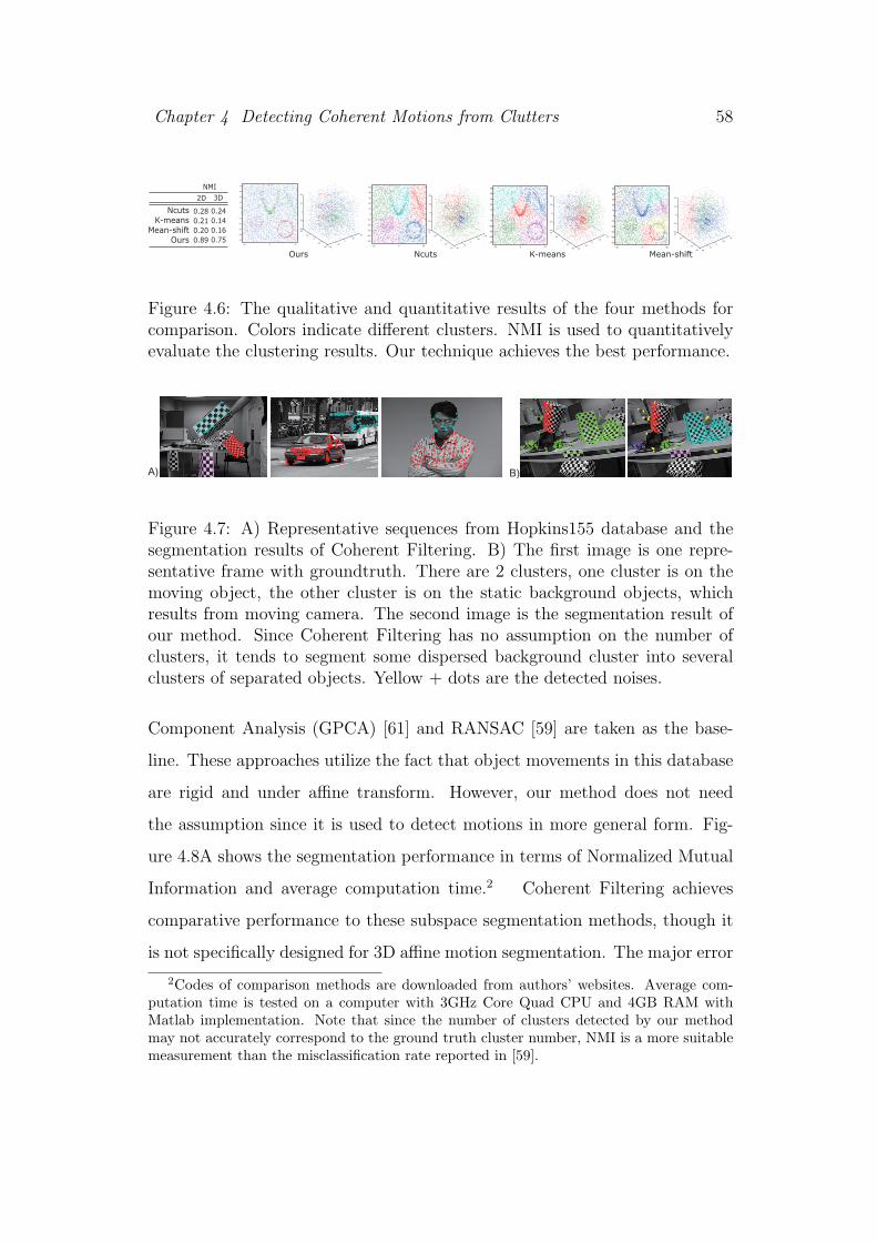
Chapter 4 Detecting Coherent Motions from Clutters 58
−50 500
−50
−40
−30
−20
−10
0
10
20
30
40
50
−40
−20
0
20
40
−40
−20
0
20
40−40
−20
0
20
40
Ncuts K-means Mean-shiftOurs
−50 0 50
−50
−40
−30
−20
−10
0
10
20
30
40
50
−50 0 50
−50
−40
−30
−20
−10
0
10
20
30
40
50
−50 0 50
−50
−40
−30
−20
−10
0
10
20
30
40
50
−40
−20
0
20
40
−40
−20
0
20
40
−40
−20
0
20
40
−40
−20
0
20
40
−40
−20
0
20
40
−40
−20
0
20
40
−40
−20
0
20
40
−40
−20
0
20
40
−40
−20
0
20
40
NcutsK-meansMean-shift
Ours
0.28
0.21
0.20
0.89
NMI
0.24
0.14
0.16
0.75
2D 3D
Figure 4.6: The qualitative and quantitative results of the four methods forcomparison. Colors indicate different clusters. NMI is used to quantitativelyevaluate the clustering results. Our technique achieves the best performance.
A) B)
Figure 4.7: A) Representative sequences from Hopkins155 database and thesegmentation results of Coherent Filtering. B) The first image is one repre-sentative frame with groundtruth. There are 2 clusters, one cluster is on themoving object, the other cluster is on the static background objects, whichresults from moving camera. The second image is the segmentation result ofour method. Since Coherent Filtering has no assumption on the number ofclusters, it tends to segment some dispersed background cluster into severalclusters of separated objects. Yellow + dots are the detected noises.
Component Analysis (GPCA) [61] and RANSAC [59] are taken as the base-
line. These approaches utilize the fact that object movements in this database
are rigid and under affine transform. However, our method does not need
the assumption since it is used to detect motions in more general form. Fig-
ure 4.8A shows the segmentation performance in terms of Normalized Mutual
Information and average computation time.2 Coherent Filtering achieves
comparative performance to these subspace segmentation methods, though it
is not specifically designed for 3D affine motion segmentation. The major error
2Codes of comparison methods are downloaded from authors’ websites. Average com-putation time is tested on a computer with 3GHz Core Quad CPU and 4GB RAM withMatlab implementation. Note that since the number of clusters detected by our methodmay not accurately correspond to the ground truth cluster number, NMI is a more suitablemeasurement than the misclassification rate reported in [59].

Chapter 4 Detecting Coherent Motions from Clutters 59
A) B)
CF
GPCA
RANSAC
TrafficArticulated
Checkboard
GPCA RANSAC CF
All sequences 0.748 0.7350.758
Average Time 1.02s 321ms7.58s
0.699 0.736 0.7440.858 0.829 0.7050.821 0.727 0.748
outlier percentage %
NMINMI
Figure 4.8: A) NMI of different methods on the Hopkins155 Database, alongwith the average computation time. Though Coherent Filtering is not specif-ically designed for 3D motion segmentation, it achieves comparative perfor-mance to other subspace segmentation methods with a better computationalefficiency. B) NMI of different methods as the function of the outlier percent-age(from 0% to 400%).
of our method comes from that our method has no assumption on the number
of motion clusters in the sequence, so that it would tend to segment some dis-
persed background cluster of ground truth into several small clusters instead
of one background cluster, as shown in Figure 4.7B. This problem is hard to
be solved using our method alone without assuming the affine transform since
these small clusters are far away to each other in space. Strictly speaking,
they do not belong to a single coherent motion, but the database ground truth
treats them as one pattern.
To further evaluate the robustness of different methods in the presence of
outliers, we add outlier trajectories from 0% to 400% into the groundtruth tra-
jectories of every 155 sequences, then test the performances of these methods.
Outlier trajectories are generated by randomly choosing initial points in the
first frame and then extending the trajectories with random walk. Figure 4.8B
shows the NMI of these methods with different outlier percentages. Coherent
Filtering works more robust with heavy noise.
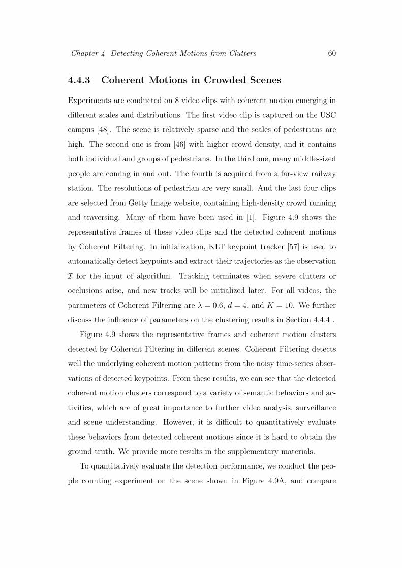
Chapter 4 Detecting Coherent Motions from Clutters 60
4.4.3 Coherent Motions in Crowded Scenes
Experiments are conducted on 8 video clips with coherent motion emerging in
different scales and distributions. The first video clip is captured on the USC
campus [48]. The scene is relatively sparse and the scales of pedestrians are
high. The second one is from [46] with higher crowd density, and it contains
both individual and groups of pedestrians. In the third one, many middle-sized
people are coming in and out. The fourth is acquired from a far-view railway
station. The resolutions of pedestrian are very small. And the last four clips
are selected from Getty Image website, containing high-density crowd running
and traversing. Many of them have been used in [1]. Figure 4.9 shows the
representative frames of these video clips and the detected coherent motions
by Coherent Filtering. In initialization, KLT keypoint tracker [57] is used to
automatically detect keypoints and extract their trajectories as the observation
I for the input of algorithm. Tracking terminates when severe clutters or
occlusions arise, and new tracks will be initialized later. For all videos, the
parameters of Coherent Filtering are λ = 0.6, d = 4, and K = 10. We further
discuss the influence of parameters on the clustering results in Section 4.4.4 .
Figure 4.9 shows the representative frames and coherent motion clusters
detected by Coherent Filtering in different scenes. Coherent Filtering detects
well the underlying coherent motion patterns from the noisy time-series obser-
vations of detected keypoints. From these results, we can see that the detected
coherent motion clusters correspond to a variety of semantic behaviors and ac-
tivities, which are of great importance to further video analysis, surveillance
and scene understanding. However, it is difficult to quantitatively evaluate
these behaviors from detected coherent motions since it is hard to obtain the
ground truth. We provide more results in the supplementary materials.
To quantitatively evaluate the detection performance, we conduct the peo-
ple counting experiment on the scene shown in Figure 4.9A, and compare

Chapter 4 Detecting Coherent Motions from Clutters 61
with trajectory clustering-based people counting method ALDENTE [48] and
Bayesian Detection counting method BayDet [9]. The experimental setting
is the same as [9]. We count the number of pedestrian detected at each key
frame (every key frame per 15 frames), and use the average people counting
error as the evaluation criteria for the three methods. Meanwhile, since at each
frame the detected clusters can be either True Positive or False Positive, and
the False Positive also can be counted as the False Negative (the undetected
one) in the number of pedestrians detected in each key frame. That makes
people counting evaluation criteria not so accurate. Thus we further evaluate
the Detection Rate (DR) and False Alarm Rate (FAR) as
DR =
∑i TPi∑iGTi
, FAR =
∑i FPi∑
i TPi + FPi
,
where TPi, FPi, and GTi are the number of True Positive, False Positive,
and groundtruth at frame i. Figure 4.10A shows the numbers of pedestrian
detected by the three methods and the groundtruth at each key frames, and
Figure 4.10B shows the average people counting error, DR, and FAR for the
three methods respectively. Coherent Filtering achieves the best performance.
On the other hand, ALDENTE and BayDet work poorly when the density of
the crowd and the level of the noise increase. As shown in Figure 4.10C, they
both fail to detect the coherent motions in crowded scenes.
4.4.4 Further Analysis of the Algorithm
Necessity of two filtering steps in the algorithm. The algorithm Co-
heFilterDet of Coherent Filtering can be divided into two steps: first remov-
ing variant neighbors and then filtering out the neighbors with low averaged
velocity correlations. As discussed in Section 4.2.2, the coherent neighbor in-
variance of spatiotemporal relationships does not guarantee that all the dots
in A are coherent dots, especially when d is small. Figure 4.11A shows the

Chapter 4 Detecting Coherent Motions from Clutters 62
clustering results directly obtained from A without thresholding when d = 6,
10, and 20 respectively, and the plot of Normalized Mutual Information (N-
MI) under different d with thresholding and without thresholding respectively.
No thresholding, when d is small there remains a significant amount of noise.
As d increases, NMI increases, which means the clustering performance is im-
proved. Then NMI with thresholding and NMI without thresholding gradually
converge. In principle, all the incoherent dots can be removed by setting a large
d, such as when d = 20. However in practice, it is difficult to obtain the cor-
respondence of dots over a long period. Thus filtering with thresholding the
averaged velocity correlations on A is necessary.
Influence of K. K decides the size of the neighborhood. Figure 4.11B
shows the clustering results with K = 5 and K = 25 on the 2D synthetic data
and the real data. When K is small, the detected coherent motion patterns
are inclined to be divided into parts. However, when K is too large, some noise
might be included. Thus the choice of K is related to the scale of coherent
motion patterns to be detected in specific videos.
4.5 Discussion and Summary
In this paper, we study the Coherent Neighbor Invariance for coherent mo-
tions and propose a simple and effective dynamic clustering technique called
Coherent Filtering for detecting coherent motions. Experimental evaluation
and comparison on synthetic and real data sets shows the existence of coher-
ent neighbor invariance in various dynamic systems and the effectiveness of
our technique under high-density noise. In the future work, we will study co-
herence neighbor invariance in a wider range of physical and biological systems
and explore more potential applications.
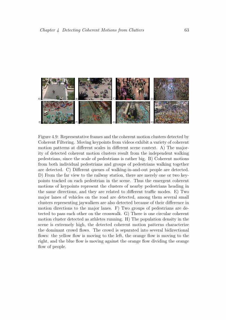
Chapter 4 Detecting Coherent Motions from Clutters 63
A) B) C) D)
E) F) G) H)
Figure 4.9: Representative frames and the coherent motion clusters detected byCoherent Filtering. Moving keypoints from videos exhibit a variety of coherentmotion patterns at different scales in different scene context. A) The major-ity of detected coherent motion clusters result from the independent walkingpedestrians, since the scale of pedestrians is rather big. B) Coherent motionsfrom both individual pedestrians and groups of pedestrians walking togetherare detected. C) Different queues of walking-in-and-out people are detected.D) From the far view to the railway station, there are merely one or two key-points tracked on each pedestrian in the scene. Thus the emergent coherentmotions of keypoints represent the clusters of nearby pedestrians heading inthe same directions, and they are related to different traffic modes. E) Twomajor lanes of vehicles on the road are detected, among them several smallclusters representing jaywalkers are also detected because of their difference inmotion directions to the major lanes. F) Two groups of pedestrians are de-tected to pass each other on the crosswalk. G) There is one circular coherentmotion cluster detected as athletes running. H) The population density in thescene is extremely high, the detected coherent motion patterns characterizethe dominant crowd flows. The crowd is separated into several bidirectionalflows: the yellow flow is moving to the left, the orange flow is moving to theright, and the blue flow is moving against the orange flow dividing the orangeflow of people.

Chapter 4 Detecting Coherent Motions from Clutters 64
Ground Truth
CF
BayDet
ALDENTE
Frame No.
Number of People
A)
ALDENTEBayesian Detection
B)
DR
FAR
CountError
0.62
0.22
1.95
CF
0.57
0.20
2.88
0.41
0.34
3.15
BayDet ALDENTE
Figure 4.10: A) The number of pedestrians detected at each key frame withrespect to Frame No., and Detection Rate(DR), False Alarm Rate(FAR),and counting error(CountError) for Coherent Filter(CF), BayDet[9], andALDENTE[48]. B) BayDet and ALDENTE fail to detect the coherent motionswhen the crowdedness and the level of noise arise.
− − −−
−
−
− − −−
−
−
d=6 d=10− − −
−
−
−
d=20
K=5 K=5K=25 K=25
A)
B)
NMI
d0 5 10 15 20 25 30 35 40
0.2
0.4
0.6
0.8
1
thresholding
no thresholding
Figure 4.11: A) Histograms of averaged velocity correlations of dots in A, andthe clustering results without thresholding, with d = 6, 10, 20 respectively. Andthe plot of NMI under different d with thresholding and without thresholding.B) Clustering results on the 2D synthetic data and the real data with K = 5and K = 25 respectively.

Chapter 5
Conclusions
This thesis mainly focuses on crowd behavior analysis, which is a promising and
interdisciplinary subject. Three projects are finished in this thesis: 1)analyzing
semantic regions from highly fragmented time-series data, 2)learning collective
crowd behavior from videos, and 3)detecting coherent motions from clutters.
We believe that this thesis is a great contribution to the research of crowd
behavior analysis.
In the first part of the thesis, we proposed a new model called Random Field
Topic model for learning semantic regions of crowded scenes from tracklets. It
effectively uses the MRF prior to capture the spatial and temporal dependen-
cy between tracklets and uses the source-sink prior to guide the learning of
semantic regions. The learned semantic regions well capture the global struc-
tures of the scenes in long range with clear semantic interpretation. They are
also able to separate different paths at fine scales with good accuracy. Both
qualitative and quantitative experimental evaluations show that it outperforms
state-of-the-art methods.
Then in the second part of the thesis, we proposed Mixture model of Dy-
namic Pedestrian-Agents to learn the collective dynamics from video sequences
in crowded scenes. The collective dynamics of pedestrians are modeled as linear
dynamic systems to capture long range moving patterns. Through modeling
the beliefs of pedestrians and the missing states of observations, it can be
65

Chapter 5 Conclusions 66
well learned from highly fragmented trajectories caused by frequent tracking
failures. By modeling the process of pedestrians making decisions on action-
s, it can not only classify collective behaviors, but also simulate and predict
collective crowd behaviors. Its effectiveness is demonstrated with various ex-
perimental results and applications on the crowded train station dataset.
At the last part of the thesis, we studied the Coherent Neighbor Invariance
for coherent motions and proposed a simple and effective dynamic clustering
technique called Coherent Filtering for detecting coherent motions. Experi-
mental evaluation and comparison on synthetic and real data sets shows the
existence of coherent neighbor invariance in various dynamic systems and the
effectiveness of our technique under high-density noise. In the future work,
we will study coherence neighbor invariance in a wider range of physical and
biological systems and explore more potential applications.
5.1 Future Works
Previous chapters show that our approaches achieve promising results on crowd
behavior analysis in real scenes. Our current approaches assume a single cam-
era view. If we need to analyze crowd behaviors in a large area, video streams
from multiple camera views have to be used. In future works, we would like
to propose some frameworks for multi-camera crowd behavior analysis, which
can group trajectories, which belong to the same activity category but are
observed in different camera views, into one cluster. The behavior patterns
of pedestrian should be jointly modeled across different video sequences. It
will be also very interesting to jointly model activities and the appearance
transformation functions under more complicated dynamic models.

Bibliography
[1] S. Ali and M. Shah. A lagrangian particle dynamics approach for crowd
flow segmentation and stability analysis. In Proc.CVPR, 2007.
[2] S. Ali and M. Shah. Floor fields for tracking in high density crowd scenes.
In Proc. ECCV, 2008.
[3] A. Anjum and A. Cavallaro. Multifeature object trajectory clustering for
video analysis. IEEE Trans. on CSVT, 2008.
[4] G. Antonini, S. Martinez, M. Bierlaire, and J. Thiran. Behavioral priors
for detection and tracking of pedestrians in video sequences. Int’l Journal
of Computer Vision, 2006.
[5] S. Atev, O. Masoud, and N. Papanikolopoulos. Learning traffic patterns
at intersections by spectral clustering of motion trajectories. In Proc.
IEEE Conf. Intell. Robots and Systems, 2006.
[6] P. Ball. Critical mass: How one thing leads to another. Farrar Straus &
Giroux, 2004.
[7] D. Blei, A. Ng, and M. Jordan. Latent dirichlet allocation. The Journal
of Machine Learning Research, 2003.
[8] E. Bonabeau. Agent-based modeling: Methods and techniques for simu-
lating human systems. PNAS, 2002.
67
[9] G. Brostow and R. Cipolla. Unsupervised bayesian detection of indepen-
dent motion in crowds. In Proc.CVPR, 2006.
[10] S. Camazine. Self-organization in biological systems. Princeton Univ Pr,
2003.
[11] D. Comaniciu and P. Meer. Mean shift: A robust approach toward feature
space analysis. IEEE Trans. on PAMI, 2002.
[12] I. Couzin. Collective cognition in animal groups. Trends in Cognitive
Sciences, 2009.
[13] W. Ge and R. Collins. Multi-target data association by tracklets with
unsupervised parameter estimation. In Proc. BMVC, 2008.
[14] D. Greenhill, J. P. Renno, J. Orwell, and G. A. Jones. Learning semantic
landscape: Embedding scene knowledge in object tracking. Real Time
Imaging, 2005.
[15] D. Helbing, I. Farkas, and T. Vicsek. Simulating dynamical features of
escape panic. Nature, 2000.
[16] D. Helbing, A. Johansson, and H. Al-Abideen. Dynamics of crowd disas-
ters: An empirical study. Physical review E, 2007.
[17] D. Helbing and P. Molnar. Social force model for pedestrian dynamics.
Physical review E, 1995.
[18] T. Hospedales, S. Gong, and T. Xiang. A markov clustering topic model
for mining behaviour in video. In Proc. ICCV, 2009.
[19] J. W. Hsieh, Y. S. H., Y. S. Chen, and W. Hu. Automatic traffic surveil-
lance system for vehicle tracking and classification. IEEE Trans. on In-
telligent Transportation Systems, 2006.
68

[20] M. Hu, S. Ali, and M. Shah. Learning motion patterns in crowded scenes
using motion flow field. In Proc. ICPR, 2008.
[21] W. Hu, T. Tan, L. Wang, and S. Maybank. A survey on visual surveillance
of object motion and behaviors. IEEE Trans. on SMC, 2004.
[22] W. Hu, X. Xiao, Z. Fu, D. Xie, T. Tan, and S. Maybank. A system for
learning statistical motion patterns. IEEE Trans. on PAMI, 2006.
[23] W. Hu, D. Xie, Z. Fu, W. Zeng, and S. Maybank. Semantic-based surveil-
lance video retrieval. IEEE Trans. on Image Processing, 2007.
[24] R. Hughes. The flow of human crowds. Annual Review of Fluid Mechanics,
2003.
[25] R. Kaucic, A. Perera, G. Brooksby, J. Kaufhold, and A. Hoogs. A unified
framework for tracking through occlusions and across sensor gaps. In
Proc.CVPR, 2005.
[26] E. Keogh and M. Pazzani. Scaling up dynamic time warping for datamin-
ing applications. In Proc. ACM SIGKDD, 2000.
[27] J. Kingman. Poisson processes. Oxford University Press, 1993.
[28] V. Lamme. The neurophysiology of figure-ground segregation in primary
visual cortex. The Journal of neuroscience, 1995.
[29] G. Le Bon. The crowd: A study of the popular mind. 1897.
[30] J. Li, S. Gong, and T. Xiang. Global behavior inference using probabilistic
latent semantic analysis. In Proc. BMVC, 2008.
[31] J. Li, S. Gong, and T. Xiang. Scene segmentation for behaviour correla-
tion. In Proc. ECCV, 2008.
69

[32] J. Li, S. Gong, and T. Xiang. Discovering multi-camera behaviour corre-
lations for on-the-fly global activity prediction and anomaly detection. In
Proc. of IEEE Int’l Workshop on Visual Surveillance, 2009.
[33] W. Liao et al. Clustering of time series data–a survey. Pattern Recognition,
2005.
[34] D. Lin, E. Grimson, and J. Fisher. Learning visual flows: A Lie algebraic
approach. In Proc.CVPR, 2009.
[35] X. Liu, L. Lin, S. Zhu, and H. Jin. Trajectory parsing by cluster sampling
in spatio-temporal graph. In Proc.CVPR, 2009.
[36] C. Loy, S. Gong, and T. Xiang. Multi-camera activity correlation analysis.
In Proc.CVPR, 2009.
[37] D. Makris and T. Ellis. Learning semantic scene models from observing
activity in visual surveillance. IEEE Trans. on SMC, 2005.
[38] R. Mehran, A. Oyama, and M. Shah. Abnormal crowd behavior detection
using social force model. In Proc.CVPR, 2009.
[39] B. Morris and M. Trivedi. A survey of vision-based trajectory learning
and analysis for surveillance. IEEE Trans. on CSVT, 2008.
[40] B. Morris and M. Trivedi. A survey of vision-based trajectory learning
and analysis for surveillance. IEEE Transactions on Circuits and Systems
for Video Technology, 2008.
[41] B. Morris and T. Trivedi. Learning trajectory patterns by clustering:
Experimental studies and comparative evaluation. In Proc.CVPR, 2009.
[42] M. Moussaid, S. Garnier, G. Theraulaz, and D. Helbing. Collective infor-
mation processing and pattern formation in swarms, flocks, and crowds.
Topics in Cognitive Science, 2009.
70

[43] W. Palma. Long-memory time series: theory and methods. Wiley-
Blackwell, 2007.
[44] J. Parrish and L. Edelstein-Keshet. Complexity, pattern, and evolutionary
trade-offs in animal aggregation. Science, 1999.
[45] S. Pellegrini, A. Ess, K. Schindler, and L. Van Gool. You’ll never walk
alone: Modeling social behavior for multi-target tracking. In Proc. ICCV,
2009.
[46] S. Pellegrini, A. Ess, and L. Van Gool. Improving data association by joint
modeling of pedestrian trajectories and groupings. Proc. ECCV, 2010.
[47] O. Petit and R. Bon. Decision-making processes: the case of collective
movements. Behavioural Processes, 2010.
[48] V. Rabaud and S. Belongie. Counting crowded moving objects. In
Proc.CVPR, 2006.
[49] I. Saleemi, K. Shafique, and M. Shah. Probabilistic modeling of scene
dynamics for applications in visual surveillance. IEEE Trans. on PAMI,
2009.
[50] P. Scovanner and M. Tappen. Learning pedestrian dynamics from the real
world. In Proc. ICCV, 2009.
[51] J. Shi and J. Malik. Normalized cuts and image segmentation. IEEE
Trans. on PAMI, 2000.
[52] R. Shumway and D. Stoffer. An approach to time series smoothing and
forecasting using the EM algorithm. Journal of time series analysis, 1982.
[53] V. Singh, B. Wu, and R. Nevatia. Pedestrian tracking by associating
tracklets using detection residuals. In Proc. IEEE Workshop on Motion
and Video Computing, 2008.
71

[54] C. Stauffer. Estimating tracking sources and sinks. In Proc.CVPR Work-
shop, 2003.
[55] A. Strehl and J. Ghosh. Cluster ensembles—a knowledge reuse framework
for combining multiple partitions. The Journal of Machine Learning Re-
search, 2003.
[56] J. Surowiecki. The wisdom of crowds: Why the many are smarter than
the few and how collective wisdom shapes business, economies, societies,
and nations. New York:Doubleday, 2004.
[57] C. Tomasi and T. Kanade. Detection and Tracking of Point Features. In
Int’l Journal of Computer Vision, 1991.
[58] A. Treuille, S. Cooper, and Z. Popovic. Continuum crowds. In ACM
SIGGRAPH, 2006.
[59] R. Tron and R. Vidal. A benchmark for the comparison of 3-d motion
segmentation algorithms. In Proc.CVPR, 2007.
[60] J. Verbeek and B. Triggs. Region classification with markov field aspect
models. In Proc.CVPR, 2007.
[61] R. Vidal, Y. Ma, and S. Sastry. Generalized principal component analysis
(gpca). IEEE Trans. on PAMI, 2005.
[62] X. Wang, K. Ma, G. Ng, and W. Grimson. Trajectory analysis and
semantic region modeling using a nonparametric bayesian model. In
Proc.CVPR, 2008.
[63] X. Wang, K. Ma, G. Ng, and W. Grimson. Trajectory analysis and se-
mantic region modeling using nonparametric hierarchical bayesian models.
Int’l Journal of Computer Vision, 2011.
72

[64] X. Wang, X. Ma, and W. Grimson. Unsupervised activity perception in
crowded and complicated scenes using hierarchical bayesian models. IEEE
Trans. on PAMI, 2008.
[65] X. Wang, X. Ma, and W. Grimson. Unsupervised activity perception in
crowded and complicated scenes using hierarchical bayesian models. IEEE
Trans. on PAMI, 2008.
[66] X. Wang, K. Tieu, and W. Grimson. Learning semantic scene models by
trajectory analysis. Proc. ECCV, 2006.
[67] X. Wang, K. Tieu, and W. Grimson. Correspondence-free activity analysis
and scene modeling in multiple camera views. IEEE Trans. on PAMI,
2008.
[68] Y. Yang, J. Liu, and M. Shah. Video scene understanding using multi-
scale analysis. In Proc. ICCV, 2009.
[69] T. Zhang, H. Lu, and S. Z. Li. Learning semantic scene models by object
classification and trajectory clustering. In Proc.CVPR, 2009.
[70] B. Zhou, X. Wang, and X. Tang. Random field topic model for semantic
region analysis in crowded scenes from tracklets. In Proc.CVPR, 2011.
[71] B. Zhou, X. Wang, and X. Tang. Understanding collective crowd behav-
iors:learning mixture model of dynamic pedestrian-agents. In Proc.CVPR,
2012.
[72] S. Zhou, D. Chen, W. Cai, L. Lyo, M. Yoke, L. Hean, F. Tian, D. Wee
Sze Ong, V. Su-Han Tay, and B. Hamilton. Crowd modeling and simula-
tion technologies. ACM Transactions on Modeling and Computer Simu-
lation, 2009.
73