modeling criminal distance decay - huduser.gov · modeling criminal distance decay the fact that...

161Cityscape: A Journal of Policy Development and Research • Volume 13, Number 3 • 2011U.S. Department of Housing and Urban Development • Office of Policy Development and Research

Cityscape

Modeling Criminal Distance DecayMike O’Leary Towson University

Abstract

Criminal distance decay is the fundamental notion that a relationship exists between the distance from an offender’s home base to a potential target location and the likelihood that the offender chooses to offend in that location. This relationship is important both for its operational effect on police agencies and on models for offender behavior. A number of factors influence the distance decay function of an offender, including the local geography and the offender’s decisionmaking process.

This article addresses a study of the interactions between the two-dimensional offense distribution that describes how offenders select targets and the corresponding one-dimensional distance decay function. It also presents the calculation of the coefficient of variation for 324 residential burglary series in Baltimore County, Maryland. These data do not support the notion that the distance decay behavior of an individual offender is governed by a number of common choices for distance decay, including the negative exponential, even allowing for the parameters to vary between offenders. Finally, the article examines geographic patterns for residential burglary in Baltimore County and the finding that, although offenses committed in rural portions of the county are commit-ted by offenders with larger travel distances, it does not appear that this variation can be explained simply by the local population density.

IntroductionDistance decay is the observed fact that offenders tend to commit more crimes closer to home than farther away. Although this qualitative fact is well known, no consensus has been reached about the correct quantitative approach to distance decay. Several researchers have put forward a number of mathematical models. Levine (2010), chapter 10, for example, discusses five different mathematical forms for distance decay built into the CrimeStat tool; CrimeStat also enables the user to create his

162 Crime and Urban Form

O’Leary

or her own empirically defined distance decay function. This notion that an offender’s crime locations are related in some meaningful way to the offender’s home location is central to the idea of geo-graphic profiling and motivates this work.

Our primary interest is in the distance decay behavior of a single offender over the course of a sin-gle crime series. We assume that the offender has a single, well-defined home base or anchor point, which can be the offender’s home, workplace, or other well-defined location of importance to the offender that serves as the origin of the offender’s base of operations. We acknowledge that this assumption does not apply to all offenders, because not all offenders meet these criteria. We also assume that each crime site has a single well-defined location, but we also acknowledge that this need not be the case for every crime. Indeed, some crimes may take place in multiple locations. As an example, in a car theft, not only is there the location from which the vehicle was stolen but also the possible chop shop location or the location where the vehicle is abandoned; also see Lu (2003) and the discussion of the “journey-after-crime.” By distance, we mean the distance from the anchor point of the offender to the location of the crime site. This distance can be measured in a number of different metrics, with Euclidean and Manhattan distance metrics being the most common but not the only reasonable choices. We also note that the distance the offender actually traveled may be at variance with the distance from the anchor point to the crime site, because it is possible that the actual journey to the crime site began at some point other than the offender’s anchor point. (See also Wiles and Costello, 2000; Santtila et al., 2008.) Finally, because we are considering the distance decay behavior of individual offenders, we note that these behaviors may vary, based on particular characteristics of the offender, the crime type, and/or the underlying local geography and landscape.

In this article, we focus on the mathematics of distance decay; in particular, we examine differ-ent quantitative models for distance decay behavior of an individual offender. We discuss the important relationships between one-dimensional models of distance and the corresponding two-dimensional models of offender behavior and show that the mathematics is responsible for some perhaps nonintuitive results. We then discuss a new method to analyze the distance decay curve for an individual offender, using aggregated data by analyzing a graph of the coefficient of variation for different offenders. Finally, we look at how geography affects the distance decay behavior of offenders, paying particular attention to the role of population density.

LiteratureClearly, the distance from the offender’s anchor point to the offense site is one of the important variables that characterize the geography of the offense(s); however, it is also important to remember that offenders select targets, not distances. In particular, the local geography and the underlying two-dimensional nature of space must be accounted for in any analysis of distance decay patterns.

Although offenders select targets, not distances, it does not mean that distance should be consid-ered to be solely a dependent variable that arises as a consequence of a particular target choice. As noted by Bernasco and Block (2009), the distance to the target may be one of the criteria that the offender uses to make the decision on where to offend.

163Cityscape

Modeling Criminal Distance Decay

The fact that the distance to the offense site is one decision variable is the only reason that tech-niques such as geographic profiling can work. If the offender selected targets without reference to their distance from the offender’s anchor point, then the crime site location would be mathemati-cally independent of the anchor point location and, in this hypothesized scenario, it would not be possible to draw inference about the anchor point location from the locations of the elements of the crime series.

In reality, it has been well established that distance decay exists, at least for crime data at the aggregate level, because this behavior has been seen in numerous studies. For example, van Kop-pen and Jansen (1998) found strong evidence of the existence of a distance decay effect in their study of 434 robberies committed by 585 offenders in the Netherlands in 1992. Bernasco (2006) analyzed and compared the distance decay behavior for 809 individual and 365 group residential burglaries in The Hague, the Netherlands, between 1996 and 2004; he found clear evidence that the behavior of both classes exhibited a distance decay pattern. Finally, Santtila, Laukkanen, and Zappalà (2007) found strong support for distance decay in their study of a collection of rapes and homicides that took place in Finland between 1992 and 2000.

Distance decay has been seen to exist in many areas of human behavior other than criminal behavior; see, for example, Gimpel et al. (2008), who studied distance decay effects in voting pat-terns and found a relationship between voting preferences and the distance from the voter to the candidate’s hometown.

In general, the question is not to know if distance decay exists, but rather to understand more about its quantitative form. In one approach to this question, Canter and Hammond (2006) evaluated a number of candidate models for distance decay, with the goal of selecting the form that provided the best results when incorporated into Dragnet.

Before we consider different possible mathematical forms for distance decay, it is important to note that the distances offenders are willing to travel depend on a number of different factors, such as the type of crime. Hesseling (1992) found that for crimes committed in residential areas of Utrecht, violent crimes and vandalism were generally committed by more local offenders than were property crimes.

Distance decay may depend on characteristics particular to an individual offender. In their study of 4,657 commercial robberies in the Netherlands in 2004 and 2005, Bernasco and Kooistra (2010) found that offenders were more than eight times more likely to offend in an area where they had lived in the past than in comparable areas where they had not lived; Bernasco (2010) obtained similar results in a study of residential burglary, theft from vehicle, robbery, and assault. The offender’s age also appears to play a role in distance decay; in a study of 41 serial burglars in St. John’s, New-foundland, Snook (2004) noted variation in the travel distances of offenders depending on the offender’s age and the value of the stolen property. Similarly, Wiles and Costello (2000) noted cor-relations between the offender’s age and the offense distance for a range of crime types in Sheffield, England. They compared these age-related effects for offenders from 1966 with offenders from 1995.

Characteristics of the criminal event itself are linked to variations in the distance offenders are willing to travel. For example, van Koppen and Jansen (1998) examined 434 commercial robberies in the Netherlands and found not only that more professional offenders were willing to travel farther but that the more difficult the target, the farther the offender(s) tended to travel. In a study


O’Leary

of 99 homicides and 56 rapes in Milan, Italy, Santtila et al. (2008) found that more instrumental crimes were correlated with larger travel distances for the offender. In another study of 40 homi-cides and 37 rapes in Finland, Santtila, Laukkanen, and Zappalà (2007) identified crime features that were correlated with distance; for example, longer distances were related to homicides that took place either in the inner city or at the victim’s home. In their analysis of a selected set of 565 rapes committed by 108 serial rapists, Warren et al. (1998) found a number of characteristics of both the offender and the crime scene that were correlated with the distance traveled by the of-fender. Finally, in their study of commercial robbery series in Greater Helsinki from 1992 through 2001, Laukkanen and Santtila (2006) found small but statistically significant correlations between particular elements of the offense and the distance traveled.

Crime rates, and especially burglary rates, are known to depend on the characteristics of the local neighborhood; for example, Bernasco and Luykx (2003) identified three neighborhood characteris-tics they termed attractiveness, opportunity, and accessibility to burglars and found that they were correlated with increased burglary rates in The Hague. In a later study of 548 residential burglaries in The Hague, Bernasco and Neiuwbeerta (2005) found a number of neighborhood characteristics associated with an increased risk of burglary, including the neighborhood’s ethnic composition and the relative number of single-family dwellings. More recently, in their study of 12,872 robber-ies in Chicago from 1996 to 1998, Bernasco and Block (2009) found that social barriers such as racial and ethnic differences and gang territorial boundaries affect the choice of a target location.

Kent and Leitner (2007) examined a mix of 97 burglary and robbery series in Baltimore County from 1994 to 1997 and compared the efficacy of circular geographic profiles with ellipses. Not only did they find that the ellipses performed better, they also found that the orientation of these ellipses were correlated with the orientation of the local road network, suggesting that the pattern of crimes might be related to the road network orientation.

When considering the geographic or geometric pattern of offense locations, it is important to con-sider direction as well as distance. In their analysis of 58 burglary series in rural Australian towns, Kocsis et al. (2002) found that the paths from the anchor point to the offense sites tended to proceed in the same direction. Similarly, Goodwill and Alison (2005) examined selected burglary series, rape series, and murder series; they also found that the paths from the anchor point to the offense site tended to lie in the same direction. See also Lu (2003), who examined the direction between the auto theft location and the vehicle recovery location for 1,600 incidents in Buffalo, New York.

One potential starting point for researchers constructing quantitative models for the distance decay behavior of offenders is to look at the distance decay graph for aggregated groups of offenders. These graphs have been generated for a large range of offense types and jurisdictions. We mention Warren et al. (1998), who provide a graph of the aggregated distance decay curve for 565 rapes committed by 108 serial rapists, and van Koppen and Jansen (1998), who provide a graph of the distribution of distances traveled to offend for 434 robberies committed by 585 offenders in the Netherlands in 1992. Snook (2004) provides an aggregate distance decay graph for residential burglars in St. John’s, Newfoundland, while Laukkanen and Santtila (2006) provide a graph of the aggregate distance decay for a commercial robbery series in Greater Helsinki, Finland, from 1992 to 2001. Canter and Hammond (2006) provide an aggregate distance decay curve for 96 selected U.S. serial murderers. This type of analysis has been done even for offenders in India; Sarangi and

165Cityscape


Youngs (2006) have aggregate distance decay graphs for serial burglars in both the Rourkela and Keonjhar districts. Santtila et al. (2008) present a distance decay curve for a collection of homi-cides, rapes, and robberies against businesses; the data in this graph are not only aggregated across offenders, but are also aggregated across offense type. Finally, in an interesting study, Lu (2003) examined the distance from the vehicle theft location to the vehicle recovery location for 1,600 incidents in Buffalo and provided an aggregate distance decay curve.

One major application of distance decay has been in the development of geographic profiling methods. Three main approaches to the geographic profiling problem use distance decay: the method of Rossmo (2000), chapter 10; the method of Canter et al. (2000); and the method of Levine (2010). (See also the approach of O’Leary, 2009.)

No consensus has been reached about the best method to evaluate the effectiveness of these systems; see the original report prepared for the National Institute of Justice (Rich and Shively, 2004), the critique of Rossmo (2005a), and the response of Levine (2005). A number of different researchers have examined the effectiveness of particular systems, however, and how to best choose the parameters that they use. For example, Sarangi and Youngs (2006) applied Dragnet to 30 Indian serial burglars committing 150 offenses and they found that Dragnet was an effective tool, while Canter and Hammond (2007) assessed the effectiveness of the Dragnet system on 96 U.S. serial murderers; they compared the search cost effectiveness of four different distance decay functions. Similarly, Laukkanen and Santtila (2006) applied CrimeStat to 76 commercial robbery series in Greater Helsinki, using empirically determined distance decay curves; they found that CrimeStat II was able to reduce the search area to roughly 5 percent of the total study area. Kent, Leitner, and Curtis (2006) constructed different distance decay functions by matching them to aggregate data and then compared their effectiveness as the distance decay function in CrimeStat, using a single serial killer in Baton Rouge, Louisiana. Not only were these comparisons made across different distance decay functions, they were also made across different distance metrics, including Euclidean, shortest path, and shortest time metrics. For a comparison of the different approaches to one another, see Paulsen (2006a, 2006b), who compared the methods with one another and with humans on crime series from Baltimore County; he found that none of these approaches were significantly better than simple centrographic measures. For a broader discussion of the comparison of geographic profiling systems with hu-mans, see Snook, Canter, and Bennell (2002); Snook, Taylor, and Bennell (2004); Rossmo (2005b); and Snook, Taylor, and Bennell (2005b). Related discussions also occur in Snook, Taylor, and Bennell (2005a); Rossmo and Filer (2005); Bennell, Snook, and Taylor (2005); and Rossmo, Filer, and Sesley (2005) and in the papers of Bennell et al. (2007) and Bennell, Taylor, and Snook (2007).

Block and Bernasco (2009) applied the Bayesian Journey to Crime method of CrimeStat 3.1 to 62 serial burglars in The Hague and evaluated its accuracy using four different measures; they found that the new Bayesian method was an improvement over distance decay methods.

Geographic profiling methods have been applied in a variety of circumstances, including applications to obscene phone calls to children in Sweden (Ebberline, 2008) and to terrorist attacks (Bennell and Corey, 2007). Bennell and Corey (2007) examined attacks by Action Directe in the 1980s in Paris and a series by the Epanastatikos Laikos Agonas in the Athens area in the 1970s and 1980s.


O’Leary

Outside the broad area of law enforcement, Buscema et al. (2009) used ideas borrowed from geo-graphic profiling to estimate the location of a point source for an outbreak of an epidemic disease. One interesting feature of their approach that has not yet been seen in criminology is that they attempt to not only model the distance from the source to a particular location, they also consider the energy expended to make the journey. Geographic profiling has also been applied to problems in ecology; Le Comber et al. (2006) and Raine, Rossmo, and Le Comber (2009) applied these techniques to problems in animal foraging, while Martin, Rossmo, and Hammerschlag (2009) examined shark predation patterns.

Brantingham and Tita (2008) discussed a model for offender motion based on ideas from foraging theory in ecology. In particular, they examined a model for offender motion based on a Lévy flight and presented the results of a number of simulations. One application of this approach to offender modeling is the geographic profiling technique of Mohler and Short (2011), which is based on a similar kinetic model for the offender’s behavior.

Finally, although our emphasis throughout is on the application of distance decay to the geographic profiling problem, distance plays a role in other questions in criminology. For example, Malleson, Evans, and Jenkins (2009) presented an agent-based model for burglary rates, which they then applied to Leeds, England. Their models incorporate a strong distance decay component, in which the agent’s likeliness of offending is inversely proportional to a function of the distance.

Dimensionality and Distance DecayCriminal distance decay is the notion that a relationship exists between the distance from an offender’s anchor point to a potential target location and the likelihood that the offender chooses to offend in that location. In this article, to make this idea mathematically precise, we define the distance decay function D to be the probability density that the offender chooses a target at a speci-fied distance r from his or her anchor point. We call this function D(r); then to find the probability P that the distance to the offense is between the numbers a and b, we simply sum the density and calculate P = ∫ a

b

0

∞

r

r + ∆r∞

–∞

∞

–∞

D(r) dr. Note that, because D(r) is a probability density and because the distance r must be nonnegative, we know that D(r) ≥ 0 for all r and ∫a

b

0

∞

r

r + ∆r∞

–∞

∞

–∞

D(r) dr = 1.

Throughout this article, we use the phrase “distance decay” because it historically has been the term used to describe this phenomenon. We will not assume that the distance decay distribution, however, be monotone decreasing, but instead we explicitly allow for the possibility that increasing the distance from the anchor point can increase or decrease the probability density that an offense takes place at that distance.

One immediate consequence of this definition of distance decay is that we are necessarily focusing our attention on the behavior of a single individual. We are explicitly allowing for the possibility that the distance decay distribution varies among offenders and that it may be influenced by the crime type, characteristics of the criminal events, the local geography, and other factors.

Because offenders select targets rather than distances, it is clear that the truly fundamental quantity that describes offender target selection is the two-dimensional probability distribution that describes how offenders select targets.

167Cityscape


Indeed, assume that points in the geographic region under study can be represented by pairs x = (x(1), x(2)), where the coordinates x(1) and x(2) represent the distances of the point x from a convenient pair of perpendicular reference axes. For simplicity in what follows, we will always as-sume that the offender’s anchor point is located at the origin in this coordinate system. We define the offender’s offense distribution T(x) = (x(1), x(2)) to be the probability density that the location x is selected by the offender as the location of an offense. Then, for any geographic region Ω, we can find the probability P that an offense occurs within Ω by calculating P = ∫∫

Ω T(x(1), x(2)) dx(1) dx(2).

Because T is a probability density, we know that T(x(1), x(2)) ≥ 0 and P = ∫a

b

0

∞

r

r + ∆r∞

–∞

∞

–∞∫

a

b

0

∞

r

r + ∆r∞

–∞

∞

–∞ T(x(1), x(2)) dx(1) dx(2) = 1.

Rossmo (2000: 197) calls a three-dimensional map of the offense distribution a jeopardy surface.

As we previously noted, the behavior of the offender, and thus the offense distribution T, can depend on factors unique to the individual committing the offenses; the crime type; the crime characteristics; and the local geographic, demographic, and other characteristics of the region.

The geometry of space imposes a fundamental relationship between the two-dimensional offense distribution T(x(1), x(2)) and the corresponding one-dimensional distance decay distribution D(r). To see this relationship, suppose we are using Euclidean distance, and we want to determine the probability P that an offense occurs at a distance between r and r + ∆r. To calculate P we sum the values of T on the annulus Ω with inner radius r and outer radius r and r + ∆r, givingP = ∫∫r≤ |x|≤r + ∆r

T(x(1), x(2)) dx(1) dx(2). If we make the simplifying assumption that the offense distribu-tion T depends only on the distance to the anchor point, then T is roughly constant on that annulus; say T(x) ≈ T(r) for r ≤ |x| ≤ r + ∆r. The area A of the annulus can be calculated simply by taking the difference of the area enclosed by the outer circle from the area enclosed by the inner circle, so A = p(r + ∆r)2 – pr2 = 2pr ∆r + p(∆r)2; thus, the probability that the offense takes place in the annulus is the product of the probability density and the area of the region, and so satisfies P ≈ (2pr∆r + p(∆r)2) T(r).

On the other hand, our definition of the distance decay distribution D(r) tells us that the probability that the offense lies at a distance between r and r + ∆r is P = ∫

a

b

0

∞

r

r + ∆r∞

–∞

∞

–∞ D(s) ds. If we make the same sim-

plifying assumption and assume that D is roughly constant on the interval [r, r + ∆r] with the value D(r), we also have the approximation P ≈ [(r + ∆r) – r]D(r) = (∆r)D(r) formed by taking the product of the length of the interval with the value of the function on that interval. Combining these two different expressions of the same quantity P, and canceling the factor Δr from both sides, we obtain the relationship D(r) ≈ (2pr + p∆r)T(r) and for small Δr, we see that D(r) ≈ (2pr)T(r).

Although this derivation proceeded via a number of mathematical approximations, these approxima-tions are not germane and it is simple to replace this argument with a formal mathematical proof. The fundamental relationship between the offense distribution and the distance decay function D(r) = 2pr T(r) holds whenever the underlying two-dimensional offense distribution T depends only on distance where Euclidean distance is being used.

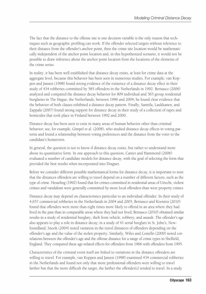
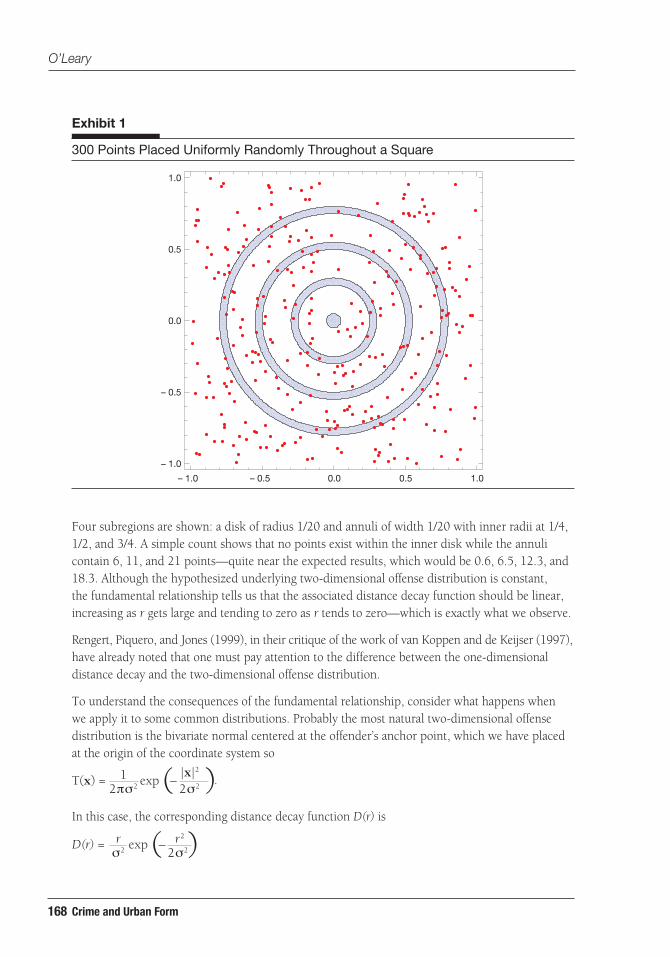
To illustrate this fundamental result, suppose we place 300 points uniformly randomly throughout the square shown in exhibit 1, effectively choosing the constant value of T=1/4 on the square [−1,1]×[−1,1].


O’Leary

Four subregions are shown: a disk of radius 1/20 and annuli of width 1/20 with inner radii at 1/4, 1/2, and 3/4. A simple count shows that no points exist within the inner disk while the annuli contain 6, 11, and 21 points—quite near the expected results, which would be 0.6, 6.5, 12.3, and 18.3. Although the hypothesized underlying two-dimensional offense distribution is constant, the fundamental relationship tells us that the associated distance decay function should be linear, increasing as r gets large and tending to zero as r tends to zero—which is exactly what we observe.

Rengert, Piquero, and Jones (1999), in their critique of the work of van Koppen and de Keijser (1997), have already noted that one must pay attention to the difference between the one-dimensional distance decay and the two-dimensional offense distribution.

To understand the consequences of the fundamental relationship, consider what happens when we apply it to some common distributions. Probably the most natural two-dimensional offense distribution is the bivariate normal centered at the offender’s anchor point, which we have placed at the origin of the coordinate system so

T(x) = exp (– )2πσ21

2σ2

|x|2

D(r) = exp (– σ2r

2σ2r2 )

.

In this case, the corresponding distance decay function D(r) is

T(x) = exp (– )2πσ21

2σ2

|x|2

D(r) = exp (– σ2r

2σ2r2 )

– 1.0 – 0.5 0.0 0.5 1.0

– 1.0

– 0.5

0.0

0.5

1.0

Exhibit 1

300 Points Placed Uniformly Randomly Throughout a Square

169Cityscape


10 2 3 4

0.1

0.2

0.3

0.4

0.5

0.6

4

2

0

– 2

– 44

20

– 2– 4

0.00

0.05

0.10

0.15

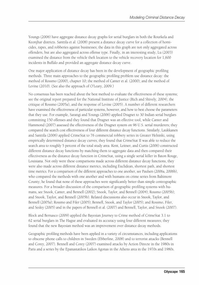
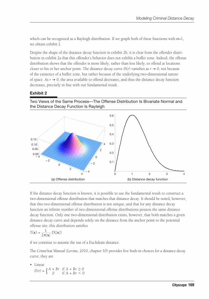
which can be recognized as a Rayleigh distribution. If we graph both of these functions with σ=1, we obtain exhibit 2.

Despite the shape of the distance decay function in exhibit 2b, it is clear from the offender distri - bution in exhibit 2a that this offender’s behavior does not exhibit a buffer zone. Indeed, the offense distribution shows that the offender is more likely, rather than less likely, to offend at locations closer to his or her anchor point. The distance decay curve D(r) vanishes as r g 0, not because of the existence of a buffer zone, but rather because of the underlying two-dimensional nature of space. As r g 0, the area available to offend decreases, and thus the distance decay function decreases, precisely in line with our fundamental result.

Exhibit 2

Two Views of the Same Process—The Offense Distribution Is Bivariate Normal and the Distance Decay Function Is Rayleigh

(a) Offense distribution (b) Distance decay function

If the distance decay function is known, it is possible to use the fundamental result to construct a two-dimensional offense distribution that matches that distance decay. It should be noted, however, that this two-dimensional offense distribution is not unique, and that for any distance decay function an infinite number of two-dimensional offense distributions possess the same distance decay function. Only one two-dimensional distribution exists, however, that both matches a given distance decay curve and depends solely on the distance from the anchor point to the potential offense site; this distribution satisfies

T(x) = D(|x|)2π|x|

2π

A + Br if A + Br ≥ 00 if A + Br < 0

1

D(r) = {

Br if r ≤ rp

Ae–Cr if r > rp.

D(r) = {

D(r) = exp (– )SA

2S2(r – r)2

2πD(r) = exp (– )r2S

A2S2

[ln(r2) – r]2–

–

if we continue to assume the use of a Euclidean distance.

The CrimeStat Manual (Levine, 2010, chapter 10) provides five built-in choices for a distance decay curve; they are

• Linear

T(x) = D(|x|)2π|x|

2π

A + Br if A + Br ≥ 00 if A + Br < 0

1

D(r) = {

Br if r ≤ rp

Ae–Cr if r > rp.

D(r) = {

D(r) = exp (– )SA

2S2(r – r)2


A2S2

[ln(r2) – r]2–

–


O’Leary

• Negative exponential

D(r) = Ae–Br

• Normal

T(x) = D(|x|)2π|x|

2π

A + Br if A + Br ≥ 00 if A + Br < 0

1

D(r) = {

Br if r ≤ rp

Ae–Cr if r > rp.

D(r) = {

D(r) = exp (– )SA

2S2(r – r)2


A2S2

[ln(r2) – r]2–

–

• Lognormal

T(x) = D(|x|)2π|x|

2π

A + Br if A + Br ≥ 00 if A + Br < 0

1

D(r) = {

Br if r ≤ rp

Ae–Cr if r > rp.

D(r) = {

D(r) = exp (– )SA

2S2(r – r)2


A2S2

[ln(r2) – r]2–

–

• Truncated negative exponential

T(x) = D(|x|)2π|x|

2π

A + Br if A + Br ≥ 00 if A + Br < 0

1

D(r) = {

Br if r ≤ rp

Ae–Cr if r > rp.

D(r) = {

D(r) = exp (– )SA

2S2(r – r)2


A2S2

[ln(r2) – r]2–

–

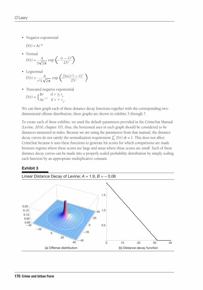
We can then graph each of these distance decay functions together with the corresponding two-dimensional offense distribution; these graphs are shown in exhibits 3 through 7.

To create each of these exhibits, we used the default parameters provided in the CrimeStat Manual (Levine, 2010, chapter 10); thus, the horizontal axes in each graph should be considered to be distances measured in miles. Because we are using the parameters from that manual, the distance decay curves do not satisfy the normalization requirement ∫ 0

∞

m

m+Δm

2

D(r) dr = 1. This does not affect CrimeStat because it uses these functions to generate hit scores for which comparisons are made between regions where these scores are large and areas where these scores are small. Each of these distance decay curves can be made into a properly scaled probability distribution by simply scaling each function by an appropriate multiplicative constant.

100 20 30 40

0.5

1.0

1.5

40

20

0

– 20

– 4040

20

0– 20

– 400.000.050.10

0.150.20

Exhibit 3

Linear Distance Decay of Levine; A = 1.9, B = − 0.06


171Cityscape


10 20 30 40

0.5

1.0

1.5

40

20

0

– 20

– 4040

20

0

– 20– 40

0.000.050.10

0.15

0.20

0

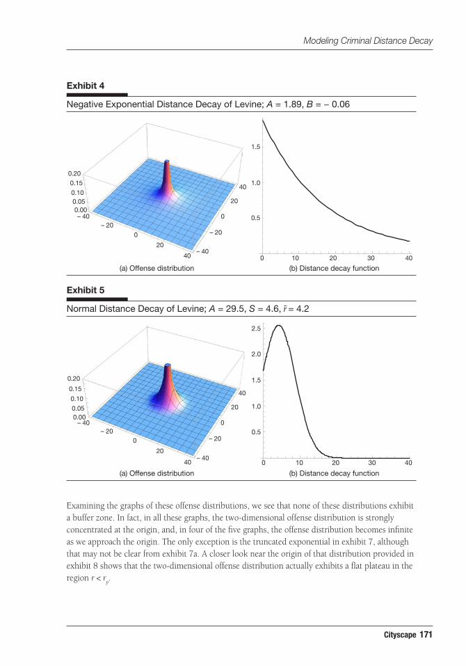
Exhibit 4

Negative Exponential Distance Decay of Levine; A = 1.89, B = − 0.06


10 20 30 40

0.5

1.0

1.5

2.0

2.5

40

20

0

– 20

– 4040

20

0– 20

– 400.000.05

0.10

0.15

0.20

0

Exhibit 5

Normal Distance Decay of Levine; A = 29.5, S = 4.6, r̄ = 4.2


Examining the graphs of these offense distributions, we see that none of these distributions exhibit a buffer zone. In fact, in all these graphs, the two-dimensional offense distribution is strongly concentrated at the origin, and, in four of the five graphs, the offense distribution becomes infinite as we approach the origin. The only exception is the truncated exponential in exhibit 7, although that may not be clear from exhibit 7a. A closer look near the origin of that distribution provided in exhibit 8 shows that the two-dimensional offense distribution actually exhibits a flat plateau in the region r < r

p.


O’Leary

Exhibit 6

Lognormal Distance Decay of Levine; A = 8.8, S = 4.6, r̄ = 4.2


0 10 20 30 40

0.2

0.4

0.6

0.8

1.0

1.2

1.4

40

20

0

– 20

– 4040

20

0– 20

– 400.00

0.050.100.150.20

Exhibit 7

Truncated Negative Exponential Distance Decay of Levine; A = 14.95, B = 34.5, C = 0.2, rp= 0.4


100 20 30 40

2

4

6

8

10

12

14

40

20

0

– 20

– 4040

20

0

– 20– 40

0

1

2

3

4

Rossmo (2000) takes a different approach; he uses a Manhattan distance metric together with a piecewise rational function for the distance decay function. An analogue of our fundamental result for the Manhattan distance is presented, however.

Suppose that we want to find the probability that an offense occurs where the Manhattan distance is between m and m + Δm. To calculate this, we need to sum the values of T over the annular region Ω outside the square |x(1)| + |x(2)| ≤ m and inside the square |x(1)| + |x(2)| ≤ m + Δm, giving us P = ∫∫m < |x(1)| + |x(2)| ≤ m + Δm

T(x(1), x(2)) dx(1) dx(2).

173Cityscape


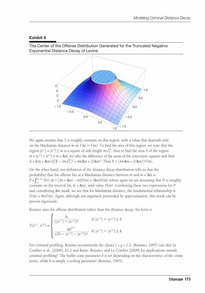
Exhibit 8

The Center of the Offense Distribution Generated for the Truncated Negative Exponential Distance Decay of Levine

We again assume that T is roughly constant on this region, with a value that depends only on the Manhattan distance m so T(x) ≈ T(m). To find the area of this region, we note that the region |x(1)| + |x(2)| ≤ m is a square of side length m

∫ 0∞

m

m+Δm

2 ; thus to find the area A of the region m < |x(1)| + |x(2)| ≤ m + Δm, we take the difference of the areas of the concentric squares and find A = ﴾(m + Δm)

∫ 0∞

m

m+Δm

2 ﴿2 – (m

∫ 0∞

m

m+Δm

2 )2 = 4mΔm + 2(Δm)2. Thus P ≈ (4mΔm + 2(Δm)2)T(m).

On the other hand, our definition of the distance decay distribution tells us that the probability that the offense lies at a Manhattan distance between m and m + Δm is P = ∫∫ 0

∞

m

m+Δm

2

D(s) ds ≈ [(m + Δm) – m]D(m) = (Δm)D(m) where again we are assuming that D is roughly constant on the interval [m, m + Δm], with value D(m). Combining these two expressions for P and considering Δm small, we see that for Manhattan distance, the fundamental relationship is D(m) = 4mT(m). Again, although our argument proceeded by approximation, this result can be proven rigorously.

Rossmo uses the offense distribution rather than the distance decay; his form is

T(x(1), x(2)) =(|x(1)| + |x(2)|) f if |x(1)| + |x(2)| ≥ b

if |x(1)| + |x(2)| ≤ b.

k

(2b – |x(1)| – |x(2)|)gkb

g–f{For criminal profiling, Rossmo recommends the choice f = g = 1.2, (Rossmo, 1995) (see also Le Comber et al., [2006], §3.2 and Raine, Rossmo, and Le Comber [2009] for applications outside criminal profiling). The buffer zone parameter b is set depending on the characteristics of the crime series, while k is simply a scaling parameter (Rossmo, 1995).

– 1.0

– 1.0

2

3

4

5

– 0.5

– 0.5

0.0

0.0

0.5

0.5

1.0

1.0


O’Leary

The offense distribution and the distance decay function are graphed in exhibit 9. Immediately seen is the effect caused by the use of the Manhattan distance rather than the Euclidean distance in that the offense distribution is no longer radially symmetric; this behavior is more clearly seen in exhibit 10, which shows the center of the offense distribution. The distance decay function decays rapidly as m g 0, although it decays very slowly for large values of m.

Exhibit 10

The Center of the Offense Distribution of Rossmo

Exhibit 9

Rossmo Model; f = g = 1.2, b = 0.3, k = 1

(a) Offense distribution (b) Distance decay function1 2 3 4 5

1

2

3

4

5

5

0

– 55

0

– 501

2

3

4

0

– 1.0

– 1.0

2

3

4

1

– 0.5

– 0.5

0.0

0.0

0.5

0.5

1.0

1.0

175Cityscape


For the values f = g = 1.2, the model of Rossmo cannot represent an offense distribution, because the tails are too large to allow for the required normalization ∫

a

b

0

∞

r

r + ∆r∞

–∞

∞

–∞∫

a

b

0

∞

r

r + ∆r∞

–∞

∞

–∞ T(x(1), x(2)) dx(1) dx(2) = 1 regardless

of the choice of the parameters b and k because we always have ∫a

b

0

∞

r

r + ∆r∞

–∞

∞

–∞∫

a

b

0

∞

r

r + ∆r∞

–∞

∞

–∞ T(x(1), x(2)) dx(1) dx(2) = ∞. One

solution to this issue would be to truncate the values of the offense distribution outside some finite but large region. One concern with this approach is that it necessarily implies that the values of the other parameters, especially the parameter k, would vary significantly with the size of the region used for the truncation.

Canter and Hammond (2006) examine four different forms for distance decay using

• LogarithmicA + B ln r if A + B ln r ≥ 0

0 if A + B ln r < 0D(r) = {

Ar2 + Br + C if Ar2 + Br + c ≥ 00 if Ar2 + Br + c < 0D(r) = {

A + Br if A + Br ≥ 00 if A + Br < 0.

D(r) = {

• Negative exponential

D(r) = Ae –Br

• Quadratic

A + B ln r if A + B ln r ≥ 00 if A + B ln r < 0D(r) = {


A + Br if A + Br ≥ 00 if A + Br < 0.

D(r) = {

• Linear

A + B ln r if A + B ln r ≥ 00 if A + B ln r < 0D(r) = {


A + Br if A + Br ≥ 00 if A + Br < 0.

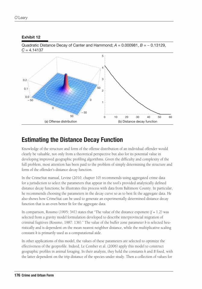
D(r) = {Two of these distributions have already been analyzed, so we provide the corresponding graphs for just the logarithmic and the quadratic distributions using the parameters selected by Canter and Hammond (2006). In their work, distances were measured in kilometers, so this represents the horizontal axes in exhibits 11 and 12.

Exhibit 11

Logarithmic Distance Decay of Canter and Hammond; A = 5.6735, B = − 1.3307


0 20 40 60 80

1

2

3

4

5

50

0

– 50

50

0

– 50

0.00

0.05

0.10


O’Leary

Exhibit 12

Quadratic Distance Decay of Canter and Hammond; A = 0.000981, B = − 0.13129, C = 4.14137

(a) Offense distribution (b) Distance decay function0 10 20 30 40 50 60

1

2

3

4

5

50

0

– 5050

0

– 500.0

0.1

0.2

Estimating the Distance Decay FunctionKnowledge of the structure and form of the offense distribution of an individual offender would clearly be valuable, not only from a theoretical perspective but also for its potential value in developing improved geographic profiling algorithms. Given the difficulty and complexity of the full problem, most attention has been paid to the problem of simply determining the structure and form of the offender’s distance decay function.

In the CrimeStat manual, Levine (2010, chapter 10) recommends using aggregated crime data for a jurisdiction to select the parameters that appear in the tool’s provided analytically defined distance decay functions; he illustrates this process with data from Baltimore County. In particular, he recommends choosing the parameters in the decay curve so as to best fit the aggregate data. He also shows how CrimeStat can be used to generate an experimentally determined distance decay function that is an even better fit for the aggregate data.

In comparison, Rossmo (1995: 341) states that “The value of the distance exponent (f = 1.2) was selected from a gravity model formulation developed to describe interprovincial migration of criminal fugitives (Rossmo, 1987: 136).” The value of the buffer zone parameter b is selected heu-ristically and is dependent on the mean nearest neighbor distance, while the multiplicative scaling constant k is primarily used as a computational aide.

In other applications of this model, the values of these parameters are selected to optimize the effectiveness of the geoprofile. Indeed, Le Comber et al. (2006) apply this model to construct geographic profiles in animal foraging. In their analysis, they hold the constants k and B fixed, with the latter dependent on the trip distance of the species under study. Then a collection of values for

177Cityscape


the exponents f and g were selected; for each exponent pair, the effectiveness of the geoprofile was evaluated to determine the best choice for the exponents. Raine, Rossmo, and Le Comber (2009) took a similar approach.

This technique of choosing distance decay parameters so as to optimize the effectiveness of the geo - profile was used earlier by Canter et al. (2000). They examined a collection of negative exponential models for distance decay and then considered variants that contained buffer zones and/or plateaus; in all, they evaluated 285 different functions for their effectiveness as geographic profiling tools.

Canter and Hammond (2006) took a hybrid approach; they selected four general models for of-fender distance decay—logarithmic, negative exponential, quadratic, and linear. For each model, they obtained the parameters that describe the model by fitting the decay curve to a collection of aggregate data. Each function generated a slightly different geographic profiling algorithm; they compared these algorithms for effectiveness.

Although all these approaches to the geographic profiling problem select a distance decay function, their focus naturally is on determining the effectiveness of geographic profiling algorithms, rather than on the problem of estimating the offense distribution or the distance decay function of an individual offender.

The primary issue in any approach to determining the distance decay behavior of an individual of-fender is one of data. Although researchers have access to data sets from a number of jurisdictions covering a wide range of crime types, the data available about any one offender are necessarily limited. In general, the series size for an individual offender is small, and although there are series in which the number of elements is large, it is possible that offenders who successfully complete a large series are special in some way. As a consequence, the individual series contain insufficient amounts of data to reliably estimate much more than some elementary parameters of the series; for example, the mean and the standard deviation of the distance from the offender’s anchor point to the crime sites.

If all offenders behaved in the same fashion, then it would be a simple matter to aggregate data collected across a suitably large set of offenders to obtain a reliable estimate of their distance decay patterns. The literature has well established the existence of significant variation in offense patterns, however, depending on characteristics of the offender, the criminal event, and the local geography.

Van Koppen and de Keijser (1997) noted that it may not be appropriate to try to draw inference about the distance decay patterns of an individual offender based on the distance decay behavior observed when aggregated across offenders. Although Rengert, Piquero, and Jones (1999) disagreed with many of the conclusions in that work, they unequivocally stated that “We do not dissent from Van Koppen and De Keijser’s assertion that researchers cannot and should not make inferences about individual behavior with data collected at the aggregate level.”

Recently, Smith, Bond, and Townsley (2009) analyzed residential burglary in Northhamptonshire, England, from 2002 to 2004. They examined 32 offenders who committed a series of at least 10 crimes; together, they committed 590 burglaries. They compared the aggregate distance decay curve for all offenders with the distance decay curves found by aggregating only offenders who


O’Leary

were alike in age and found significant qualitative differences among these graphs, providing direct evidence that offenders do not in general possess the same distance decay patterns. In fact, they found that roughly two-thirds of the variation in offense distances can be ascribed to variations among offenders, rather than to variation in an individual offender.

Townsley and Sidebottom (2010) then examined a larger data set of residential and nonresidential burglaries involving more than 1,300 offenders and 16,000 offenses. They found that nearly one-half of the variation in offense distances could be explained by variation among offenders.

Given these facts, is it possible to estimate the quantitative behavior of an individual from the available aggregate data?

Coefficient of VariationThe next step is to analyze a data set provided by the Baltimore County Police Department. Baltimore County is a primarily suburban county in Maryland that borders Baltimore City; it forms a collar around the west, north, and east boundaries of the city. The U.S. Census Bureau’s 2009 estimate for the population of Baltimore County is 789,814. The portion of the county near the border with Baltimore City and inside or near the Baltimore Beltway, or Interstate 695 (I–695), is primarily urban and suburban, with much of the remainder of the county being rural. The county contains no other municipal governments; however, a number of communities have well-defined names, including Towson, Halethorpe, Dundalk, Owings Mills, Cockeysville, Baldwin, and Monk-ton. A map of Baltimore County is provided in exhibit 13.

Our data set for analysis consists of solved residential burglaries committed in Baltimore County between 1986 and 2008. For each incident, we identified the location of the offense and the loca-tion of the home of the offender; we also have basic demographic information about the offender, including the age, sex, race, and date of birth of the offender. The data set contains 5,859 offender-offense pairs, with 2,890 individual offenders committing 4,542 separate burglaries. The data set contains 324 series of four or more burglaries committed by the same offender.

We identified individual offenders by matching the provided demographic information and home location. It is possible that two or more different individuals may have the same demographic information and the same home address; it is also possible that a single individual offender could possess different home addresses at different times. The data set contains no instances, however, in which the date of birth matched and the home address did not, suggesting that these concerns are likely to have little practical effect. The home address recorded in the data set may not be the actual anchor point for the offender at the time of the offenses. A series is identified solely as a collection of burglaries committed by the same offender; as a consequence, we do not account for confounding factors such as the presence of multiple offenders.

Of the 324 identified series, the mean length of a series is 8.1 crimes, with a median of 6 and a maximum of 54. A histogram of the number of series as a function of the series length is provided in exhibit 14.

179Cityscape


Exhibit 13

Exhibit 14

A Map of Baltimore County

Baltimore County Residential Burglaries, 1986–2008: Number of Series As a Function of the Length of the Series

100 20 30 40 50Series length

50

100

150

Num

ber

of s

erie

s


O’Leary

Suppose that the distance decay behavior of an individual offender is governed by a negative exponential distribution in the usual form

A(r) = D(r| ) µ( ) d = µ( ) d

A(r) = p1D(r|

1 ) + p

2D(r|

2) = e –r/ 1 + e –r/ 2

D(r| ) = e –r/ 1

p1

e –r/ 1

1

∫ 0∞ ∫ 0∞

p2

2

,

but that the parameter β may be different for each offender. Then we do not expect that the distribution of offense distances aggregated across all offenders satisfies a negative exponential distribution. To illustrate this, suppose that offenders fall into two categories, with the fraction p

1

with parameter β1 and the fraction p

2 with parameter β

2. Then it is clear to see that, sampling

across offenders, we obtain the aggregate distribution

A(r) = D(r| ) µ( ) d = µ( ) d

A(r) = p1D(r|

1 ) + p

2D(r|

2) = e –r/ 1 + e –r/ 2

D(r| ) = e –r/ 1

p1

e –r/ 1

1

∫ 0∞ ∫ 0∞

p2

2,

which is not a negative exponential. In general, if the parameter β is distributed across offenders according to a probability density μ(β), then the distribution of offense distances A(r) aggregated across offenders would then satisfy

A(r) = D(r| ) µ( ) d = µ( ) d

A(r) = p1D(r|

1 ) + p

2D(r|

2) = e –r/ 1 + e –r/ 2

D(r| ) = e –r/ 1

p1

e –r/ 1

1

∫ 0∞ ∫ 0∞

p2

2

.

Although each individual offense series is far too small to reliably estimate the offense distribution or even the distance decay function of an individual offender, we can estimate both the mean and the standard deviation of the distance from the home location to the offense site for each series. Doing so lets us estimate the coefficient of variation of each series, which is defined to be the ratio of the standard deviation to the mean of a distribution.

We can also calculate the mean and standard deviation of the negative exponential distribution; both the mean and the standard deviation are β, and hence the coefficient of variation is identi-cally 1. The significance of this result is that the coefficient of variation does not depend on the parameter β. Thus, if all individual offenders select targets according to a negative exponential, then we expect that the sample coefficient of variation should be roughly 1, regardless of how the parameter β is distributed across offenders in the population.

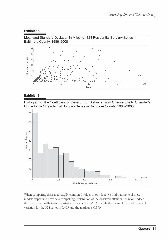
To test this hypothesis, we plotted the mean and the standard deviation of the distance from the crime site to the offender’s home in exhibit 15. If individual offenders all have a negative exponen-tial distance decay function, then we would expect these points to lie close to the line with slope 1.

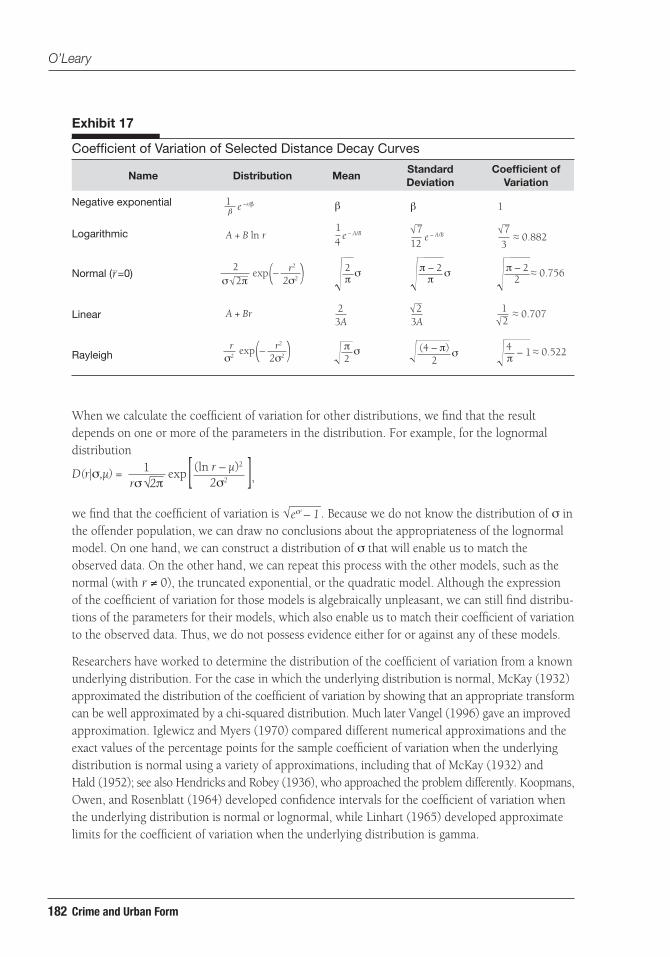
Examining the graph, it is clear that the typical ratio of standard deviation to mean is much less than unity. To investigate this ratio further, we plot a histogram of the coefficients of variation for the distance decay function of our serial offenders and obtain exhibit 16, which confirms our observation that the coefficient of variation is less than unity for nearly all of our observations and suggests that the negative exponential model for distance decay is not a good fit for the behavior of individual offenders.

We can also calculate the coefficient of variation for the other commonly chosen models for offender distance decay. In many cases, the coefficient of variation is independent of all the parameters in the distribution, letting us repeat this analysis. Doing so, we find that the coefficient of variation is constant for the logarithmic model (0.882), the normal model with r = 0, (0.756), the linear model (0.707), and the Rayleigh model (0.522). These results are summarized in exhibit 17.

181Cityscape


5 10 15 20Mean

1

2

3

4

5

6

Sta

ndar

d d

evia

tion

0

Exhibit 15

Mean and Standard Deviation in Miles for 324 Residential Burglary Series in Baltimore County, 1986–2008

0.5 1.0 1.5 2.0

Coefficient of variation

10

20

30

40

50

60

70

Num

ber

of s

erie

s

0

Exhibit 16

Histogram of the Coefficient of Variation for Distance From Offense Site to Offender’s Home for 324 Residential Burglary Series in Baltimore County, 1986–2008

When comparing these analytically computed values to our data, we find that none of these models appears to provide a compelling explanation of the observed offender behavior. Indeed, the theoretical coefficients of variation all are at least 0.522, while the mean of the coefficients of variation for the 324 series is 0.455 and the median is 0.390.


O’Leary

When we calculate the coefficient of variation for other distributions, we find that the result depends on one or more of the parameters in the distribution. For example, for the lognormal distribution

D(r|σ,µ) = exp[ ]1rσ 2π

(ln r – µ)2

2σ2

eσ2 – 1

,

we find that the coefficient of variation is

D(r|σ,µ) = exp[ ]1rσ 2π

(ln r – µ)2

2σ2

eσ2 – 1 . Because we do not know the distribution of σ in the offender population, we can draw no conclusions about the appropriateness of the lognormal model. On one hand, we can construct a distribution of σ that will enable us to match the observed data. On the other hand, we can repeat this process with the other models, such as the normal (with r ≠ 0), the truncated exponential, or the quadratic model. Although the expression of the coefficient of variation for those models is algebraically unpleasant, we can still find distribu-tions of the parameters for their models, which also enable us to match their coefficient of variation to the observed data. Thus, we do not possess evidence either for or against any of these models.

Researchers have worked to determine the distribution of the coefficient of variation from a known underlying distribution. For the case in which the underlying distribution is normal, McKay (1932) approximated the distribution of the coefficient of variation by showing that an appropriate transform can be well approximated by a chi-squared distribution. Much later Vangel (1996) gave an improved approximation. Iglewicz and Myers (1970) compared different numerical approximations and the exact values of the percentage points for the sample coefficient of variation when the underlying distribution is normal using a variety of approximations, including that of McKay (1932) and Hald (1952); see also Hendricks and Robey (1936), who approached the problem differently. Koopmans, Owen, and Rosenblatt (1964) developed confidence intervals for the coefficient of variation when the underlying distribution is normal or lognormal, while Linhart (1965) developed approximate limits for the coefficient of variation when the underlying distribution is gamma.

Exhibit 17

Name Distribution MeanStandard Deviation

Coefficient of Variation

Coefficient of Variation of Selected Distance Decay Curves

Negative exponential

Logarithmic

Normal (r=0)

Linear

Rayleigh

e –r/β

e – A/BA + B ln r

r2

2σ2(– )

A + Br

1 1

23A

2πσ

2

23A

3

β β

2πexp

σ

r2

2σ2(– )rσ2

exp

21 ≈ 0.707

712

7e – A/B

41

π – 2π

σ π – 22≈ 0.756

≈ 0.882

4 – 1π

≈ 0.5222π σ

2(4 – π) σ

183Cityscape


In particular, although we have qualitative evidence to suggest that none of the models in exhibit 17 is sufficient to describe the distance decay behavior of offenders, we are unable to present a quantita-tive estimate of the potential significance of this statement. We are not the first researchers to apply the coefficient of variation to problems of distance decay; see Smith, Bond, and Townsley (2009), who calculated the coefficients of variation for the different aggregated samples provided in Snook (2004).

The Impact of GeographySo far, we have considered the offense distribution and the corresponding distance decay function from the point of view of an individual offender. It is possible, however, even likely, that the distance decay function varies with location. This idea is not new; for example, Eldridge and Jones (1991) discuss how the parameters in a distance decay model may vary across geography. In particular, they consider how the parameters in a gravity-based model might also vary across space, and so allow for and estimate quadratic variation in the parameters.

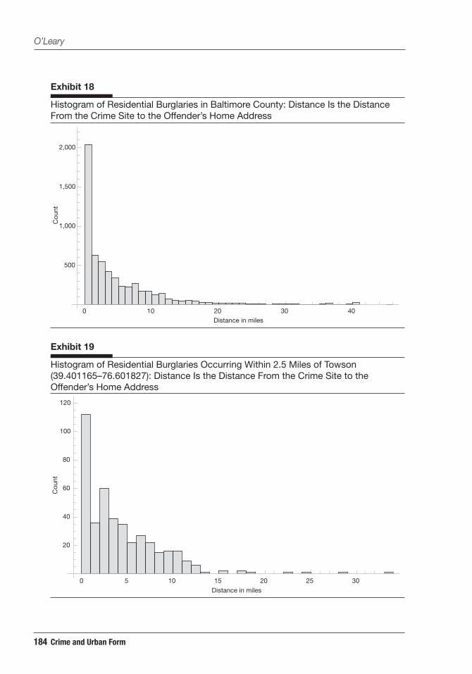
To see how geography might impact distance decay behavior, let us start by examining the aggre-gate distance decay curve for the 5,859 offender-offense pairs for residential burglaries committed in Baltimore County. In particular, we plot a histogram of the number of residential burglary pairs against the distance the offender traveled to commit the crime, which renders exhibit 18.

To understand the role of geography, we repeat this exercise but, instead of examining all of the incidents in Baltimore County, we first select a geographic region and then select only the offenses that occurred in that region. For example, let us first examine the aggregate distance decay curve for all of the studied residential burglaries that occurred within a 2.5-mile radius of Towson, where, for definiteness, we set the center of Towson to have latitude/longitude 39.401165/-76.601827; see also the map in exhibit 13. Doing so, we obtained exhibit 19.

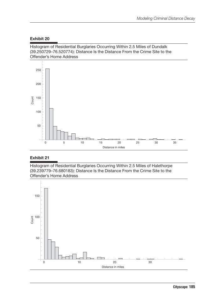
Comparing exhibits 16 and 18, we find no significant qualitative difference between the structures of histograms. We can repeat the process and examine the histogram of the aggregate distance decay curves for crimes committed within 2.5 miles of Dundalk (exhibit 20) and within 2.5 miles of Halethorpe (exhibit 21). As with Towson, these towns are urban/suburban areas within the Baltimore Beltway (I–695). Not only are these areas similar in their urban structure, the aggregate distance decay functions for residential burglaries in these areas show many qualitative similarities. Indeed, they all show that most crimes occur very close to the offender’s residence and that the number of crimes decreases as the distance between the offender’s home and the crime site increases.

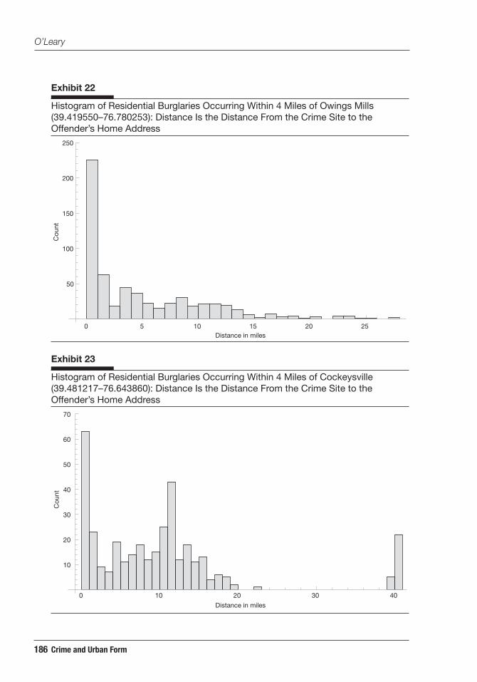
Next, we examine the aggregate distance decay curves for two areas farther removed from the urban core. Owings Mills and Cockeysville are each suburban communities of roughly 20,000 people that lie on the major roads leading radially outward from Baltimore City (see the map in exhibit 13). Because of the smaller population density for these communities, we expand the size of the local region and, in exhibits 22 and 23, we plot the histogram of the number of residential burglaries versus the distance from the crime site to the offender’s home for crimes committed within 4 miles of Owings Mills (exhibit 22) and Cockeysville (exhibit 23).


O’Leary

50 10 15 20 25 30

20

40

60

80

100

120

Distance in miles

Cou

nt

0 10 20 30 40

500

1,000

1,500

2,000

Distance in miles

Cou

nt

Exhibit 18

Exhibit 19

Histogram of Residential Burglaries in Baltimore County: Distance Is the Distance From the Crime Site to the Offender’s Home Address

Histogram of Residential Burglaries Occurring Within 2.5 Miles of Towson (39.401165–76.601827): Distance Is the Distance From the Crime Site to the Offender’s Home Address

185Cityscape


0 10 20 30

50

100

150

Distance in miles

Cou

nt

0 5 10 15 20 25 30 35

50

100

150

200

250

Distance in miles

Cou

nt

Exhibit 20

Exhibit 21

Histogram of Residential Burglaries Occurring Within 2.5 Miles of Dundalk (39.250729–76.520774): Distance Is the Distance From the Crime Site to the Offender’s Home Address

Histogram of Residential Burglaries Occurring Within 2.5 Miles of Halethorpe (39.239779–76.680183): Distance Is the Distance From the Crime Site to the Offender’s Home Address


O’Leary

0 5 10 15 20 25

50

100

150

200

250

Distance in miles

Cou

nt

100 20 30 40

10

20

30

40

50

60

70

Distance in miles

Cou

nt

Exhibit 22

Exhibit 23

Histogram of Residential Burglaries Occurring Within 4 Miles of Owings Mills (39.419550–76.780253): Distance Is the Distance From the Crime Site to the Offender’s Home Address

Histogram of Residential Burglaries Occurring Within 4 Miles of Cockeysville (39.481217–76.643860): Distance Is the Distance From the Crime Site to the Offender’s Home Address

187Cityscape


50 10 15 20 25

2

4

6

8

10

12

Distance in miles

Cou

nt

At this point we begin to notice significant qualitative differences in the shape and structure of the aggregate distance decay histograms. The histogram for Owings Mills remains similar to the histograms for Towson, Dundalk, and Halethorpe in that all these histograms have a strong peak at the origin, with most crimes committed close to the offender’s home address. One difference is that the Owings Mills histogram does not quickly decay as the distance increases; indeed, the offense count decays only very slowly, if at all, for crimes at distances between 1 and 10 miles from the offender’s home address.

These differences, however, pale in comparison with the differences observed in the histogram for burglaries committed near Cockeysville. The largest number of crimes was committed by offenders whose home address is close to the crime site; however, a significant second peak occurs for crimes in which the distance to the offender’s home address is 11 to 12 miles. That graph also shows that a significant number of offenses were committed by offenders whose home address was more than 40 miles from the crime site. Even if we disregard this latter peak as being somehow unrepresenta-tive, we still see clear differences between the aggregate distance decay behavior in Cockeysville versus the observed communities near the urban core.

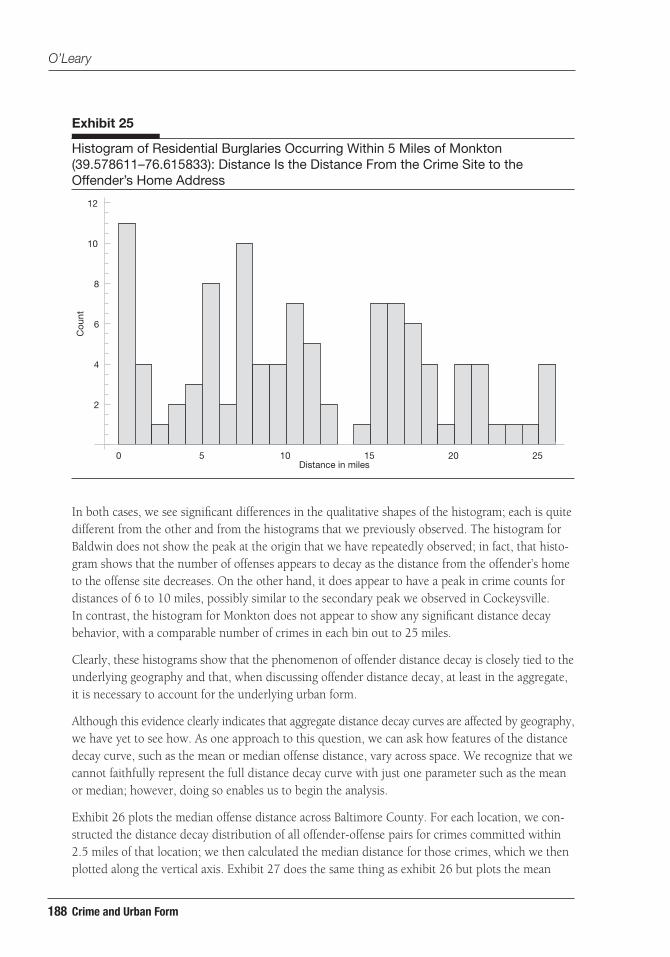
We continue by examining the rural communities of Baldwin and Monkton and, in exhibits 24 and 25, we plot the histogram of the number of residential burglaries versus the distance between the crime site and the offender’s home address for offenses within 5 miles of Baldwin (exhibit 24) and Monkton (exhibit 25). We once again expanded the radius around the community, now to 5 miles, to ensure that the region contained enough crime to create a reasonable histogram.

Exhibit 24

Histogram of Residential Burglaries Occurring Within 5 Miles of Baldwin (39.494772–76.470556): Distance Is the Distance From the Crime Site to the Offender’s Home Address


O’Leary

50 10 15 20 25

2

4

6

8

10

12

Distance in miles

Cou

nt

Exhibit 25

Histogram of Residential Burglaries Occurring Within 5 Miles of Monkton (39.578611–76.615833): Distance Is the Distance From the Crime Site to the Offender’s Home Address

In both cases, we see significant differences in the qualitative shapes of the histogram; each is quite different from the other and from the histograms that we previously observed. The histogram for Baldwin does not show the peak at the origin that we have repeatedly observed; in fact, that histo-gram shows that the number of offenses appears to decay as the distance from the offender’s home to the offense site decreases. On the other hand, it does appear to have a peak in crime counts for distances of 6 to 10 miles, possibly similar to the secondary peak we observed in Cockeysville. In contrast, the histogram for Monkton does not appear to show any significant distance decay behavior, with a comparable number of crimes in each bin out to 25 miles.

Clearly, these histograms show that the phenomenon of offender distance decay is closely tied to the underlying geography and that, when discussing offender distance decay, at least in the aggregate, it is necessary to account for the underlying urban form.

Although this evidence clearly indicates that aggregate distance decay curves are affected by geography, we have yet to see how. As one approach to this question, we can ask how features of the distance decay curve, such as the mean or median offense distance, vary across space. We recognize that we cannot faithfully represent the full distance decay curve with just one parameter such as the mean or median; however, doing so enables us to begin the analysis.

Exhibit 26 plots the median offense distance across Baltimore County. For each location, we con - structed the distance decay distribution of all offender-offense pairs for crimes committed within 2.5 miles of that location; we then calculated the median distance for those crimes, which we then plotted along the vertical axis. Exhibit 27 does the same thing as exhibit 26 but plots the mean

189Cityscape


– 76.8

– 76.6

– 76.4

Longitude

39.4

39.6

Latitude0

10

20

30

Meandistance

– 76.8

– 76.6

– 76.4

Longitude

39.4

39.6

Latitude0

10

20

30

Mediandistance

Exhibit 26

Exhibit 27

Median Distance in Miles Between the Offense Site and the Offender’s Home Address for Offenses Committed Within 2.5 Miles of That Location

Mean Distance in Miles Between the Offense Site and the Offender’s Home Address for Offenses Committed Within 2.5 Miles of That Location


O’Leary

– 76.8

– 76.6

– 76.4

Longitude

39.2

39.4

39.6

Latitude

0

2,000

4,000

Population

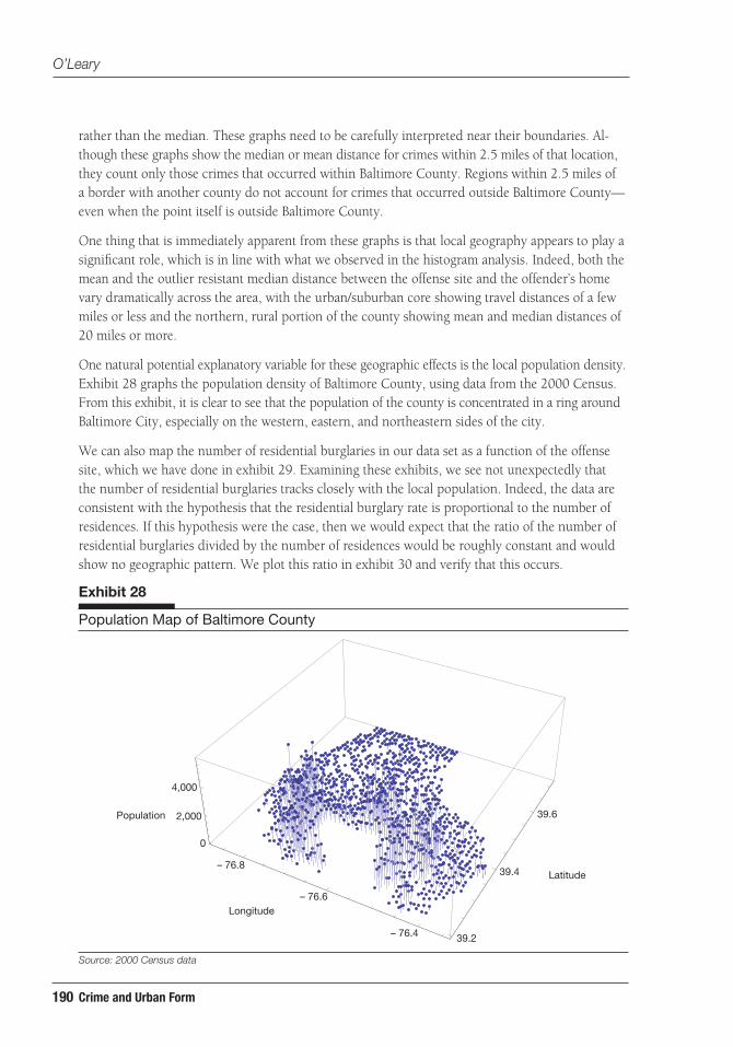
rather than the median. These graphs need to be carefully interpreted near their boundaries. Al-though these graphs show the median or mean distance for crimes within 2.5 miles of that location, they count only those crimes that occurred within Baltimore County. Regions within 2.5 miles of a border with another county do not account for crimes that occurred outside Baltimore County—even when the point itself is outside Baltimore County.

One thing that is immediately apparent from these graphs is that local geography appears to play a significant role, which is in line with what we observed in the histogram analysis. Indeed, both the mean and the outlier resistant median distance between the offense site and the offender’s home vary dramatically across the area, with the urban/suburban core showing travel distances of a few miles or less and the northern, rural portion of the county showing mean and median distances of 20 miles or more.

One natural potential explanatory variable for these geographic effects is the local population density. Exhibit 28 graphs the population density of Baltimore County, using data from the 2000 Census. From this exhibit, it is clear to see that the population of the county is concentrated in a ring around Baltimore City, especially on the western, eastern, and northeastern sides of the city.

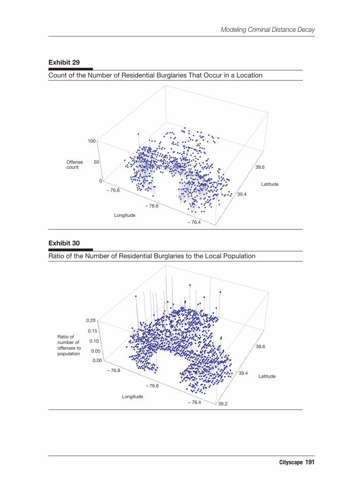
We can also map the number of residential burglaries in our data set as a function of the offense site, which we have done in exhibit 29. Examining these exhibits, we see not unexpectedly that the number of residential burglaries tracks closely with the local population. Indeed, the data are consistent with the hypothesis that the residential burglary rate is proportional to the number of residences. If this hypothesis were the case, then we would expect that the ratio of the number of residential burglaries divided by the number of residences would be roughly constant and would show no geographic pattern. We plot this ratio in exhibit 30 and verify that this occurs.

Exhibit 28

Population Map of Baltimore County

Source: 2000 Census data

191Cityscape


– 76.8

– 76.6

– 76.4

Longitude

39.4

39.6

Latitude0

50

100

Offensecount

– 76.8

– 76.6

– 76.4Longitude

39.2

39.4

39.6

Latitude

0.00

0.05

0.10

0.15

0.20

Ratio of number of offenses to population

Exhibit 29

Exhibit 30

Count of the Number of Residential Burglaries That Occur in a Location

Ratio of the Number of Residential Burglaries to the Local Population


O’Leary

0

10

20

30

40

Average offensedistance

0

1,000

2,000

3,000

4,000

Local population

0

20

40

Count

To better understand the effect of population on the aggregate distance decay histogram, let us add a third dimension to the graph and aggregate the crimes, not only by the distance from the crime site to the offender’s home but also by the population density of the region where the offense was committed. Doing so, we obtain exhibit 31.

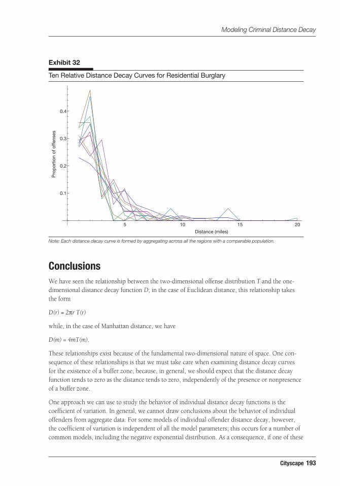
When examining the sections of this histogram for fixed population, we see that the distance decay behavior seems to vary with the local population; regions with smaller populations appear to possess a smaller number of offenders willing to travel a long distance to offend than regions with larger populations. The histogram also clearly shows many more regions with a small local popula-tion than regions with a large local population. Thus, the longer tails in the distance decay sections noted in the histogram may be caused by the fact that they are drawing from a larger sample. To confirm this hypothesis, we can graph the distance decay curves for regions aggregated across comparable populations, but, to account for the different number of offenses in regions of different population, we graph only the relative fraction, which we have done in exhibit 32.

The rough agreement of these curves with one another suggests that, whatever relationship exists between local geography and distance decay patterns, the interaction does not appear to be medi-ated by the population density of the target location.

Exhibit 31

Count of the Number of Residential Burglaries, Sorted by Both Mean Offender Travel Distance and Population of the Burglary Location

193Cityscape


5 10 15 20

Distance (miles)

0.1

0.2

0.3

0.4

Pro

por

tion

of o

ffen

ses

ConclusionsWe have seen the relationship between the two-dimensional offense distribution T and the one-dimensional distance decay function D; in the case of Euclidean distance, this relationship takes the form

D(r) = 2pr T(r)

while, in the case of Manhattan distance, we have

D(m) = 4mT(m).

These relationships exist because of the fundamental two-dimensional nature of space. One con-sequence of these relationships is that we must take care when examining distance decay curves for the existence of a buffer zone, because, in general, we should expect that the distance decay function tends to zero as the distance tends to zero, independently of the presence or nonpresence of a buffer zone.

One approach we can use to study the behavior of individual distance decay functions is the coefficient of variation. In general, we cannot draw conclusions about the behavior of individual offenders from aggregate data. For some models of individual offender distance decay, however, the coefficient of variation is independent of all the model parameters; this occurs for a number of common models, including the negative exponential distribution. As a consequence, if one of these

Exhibit 32

Ten Relative Distance Decay Curves for Residential Burglary

Note: Each distance decay curve is formed by aggregating across all the regions with a comparable population.


O’Leary

models held for all offenders, then we should see roughly constant coefficients of variation across offenders. An exploratory data analysis of Baltimore County residential burglaries shows significant variation in the coefficient of variation, however, suggesting that none of these models, including the negative exponential model, are appropriate for the modeling of individual-level distance decay.

Finally, we examined the effect of geography on aggregate-level distance decay curves. In our study of Baltimore County residential burglaries, we found that the aggregate distance decay curves var-ied significantly depending on the locations of the crime sites that were aggregated. In particular, we found that the average distance between the crime site and the offender’s home address was dramatically larger in the rural portions as opposed to the more urban and suburban portions of the county. We performed an exploratory analysis to see if this variation could be explained by dif-ferences in local population density, but the results of our analysis did not support this hypothesis.

Acknowledgments

The author thanks the Baltimore County Police Department and Phil Canter for graciously agreeing to provide the data used in this study. This work is partially supported by the National Institute of Justice through grant 2009-SQ-B9-K014.

Author

Mike O’Leary is the director of the School of Emerging Technology and a professor in the Department of Mathematics at Towson University.

References

Bennell, Craig, and Shevaun Corey. 2007. “Geographic Profiling of Terrorist Attacks.” In Criminal Profiling: International Theory, Research, and Practice, edited by Richard N. Kocsis. Totowa, NJ: Humana Press: 189–203.

Bennell, Craig, Brent Snook, and Paul Taylor. 2005. “Geographic Profiling—The Debate Continues,” Blue Line Magazine, October: 34–36.

Bennell, Craig, Brent Snook, Paul Taylor, Shevaun Corey, and Julia Keyton. 2007. “It’s No Riddle, Choose the Middle,” Criminal Justice and Behavior 34 (1): 119–132.

Bennell, Craig, Paul Taylor, and Brent Snook. 2007. “Clinical Versus Actuarial Geographic Profiling Strategies: A Review of the Research,” Police Practice and Research 8 (4): 335–345.

Bernasco, Wim. 2010. “Modeling Micro-Level Crime Location Choice: Application of the Discrete Choice Framework to Crime at Places,” Journal of Quantitative Criminology 26: 113–138.

———. 2006. “Co-Offending and the Choice of Target Areas in Burglary,” Journal of Investigative Psychology and Offender Profiling 3: 139–155.

Bernasco, Wim, and Richard Block. 2009. “Where Offenders Choose To Attack: A Discrete Choice Model of Robberies in Chicago,” Criminology 47 (1): 93–130.

195Cityscape


Bernasco, Wim, and Thessa Kooistra. 2010. “Effects of Residential History on Commercial Robbers’ Crime Location Choices,” European Journal of Criminology 7 (4): 251–265.

Bernasco, Wim, and Floor Luykx. 2003. “Effects of Attractiveness, Opportunity, and Accessibility to Burglars on Residential Burglary Rates of Urban Neighborhoods,” Criminology 41 (3): 981–1001.

Bernasco, Wim, and Paul Neiuwbeerta. 2005. “How Do Residential Burglars Select Target Areas?” The British Journal of Criminology 44: 296–315.

Block, Richard, and Wim Bernasco. 2009. “Finding a Serial Burglar’s Home Using Distance Decay and Conditional Origin-Destination Patterns: A Test of Empirical Bayes Journey-to-Crime Estimation in The Hague,” Journal of Investigative Psychology and Offender Profiling 6: 187–211.

Brantingham, P. Jeffrey, and George Tita. 2008. “Offender Mobility and Crime Pattern Formation From First Principles.” In Artificial Crime Analysis Systems: Using Computer Simulations and Geographic Information Systems, edited by Lin Liu and John Eck. Hershey, PA: Idea Press: 193–208.

Buscema, Massimo, Enzo Grossi, Marco Breda, and Tom Jefferson. 2009. “Outbreaks Source: A New Mathematical Approach To Identify Their Possible Location,” Physica A 388: 4736–4762.

Canter, David, Toby Coffey, Malcolm Huntley, and Christopher Missen. 2000. “Predicting Serial Killers’ Home Base Using a Decision Support System,” Journal of Quantitative Criminology 16 (4): 457–478.

Canter, David, and Laura Hammond. 2007. “Prioritizing Burglars: Comparing the Effectiveness of Geographical Profiling Methods,” Police Practice and Research 8 (4): 371–384.

———. 2006. “A Comparison of the Efficacy of Different Decay Functions in Geographical Profiling for a Sample of U.S. Serial Killers,” Journal of Investigative Psychology and Offender Profiling 3: 91–103.

Ebberline, Jessica. 2008. “Geographical Profiling Obscene Phone Calls—A Case Study,” Journal of Investigative Psychology and Offender Profiling 5: 93–105.

Eldridge, J. Douglas, and John Paul Jones. 1991. “Warped Space: A Geography of Distance Decay,” Professional Geographer 43 (4): 500–511.

Gimpel, James G., Kimberly A. Karnes, John McTague, and Shanna Pearson-Merkowitz. 2008. “Distance-Decay in the Political Geography of Friends-and-Neighbors Voting,” Political Geography 27: 231–252.

Goodwill, Alasdair M., and Laurence J. Alison. 2005. “Sequential Angulation, Spatial Dispersion, and Consistency of Distance Attack Patterns From Home in Serial Murder, Rape, and Burglary,” Psychology, Crime & Law 11 (2): 161–176.

Hald, Anders. 1952. Statistical Theory With Engineering Application. New York: Wiley.

Hendricks, Walter A., and Kate W. Robey. 1936. “Sampling Distribution of the Coefficient of Variation,” The Annals of Mathematical Statistics 7 (3): 129–132.


O’Leary

Hesseling, Rene B.P. 1992. “Using Data on Offender Mobility in Ecological Research,” Journal of Quantitative Criminology 8 (1): 95–112.

Iglewicz, Boris, and Raymond H. Myers. 1970. “Comparisons of Approximations to the Percentage Points of the Sample Coefficient of Variation,” Technometrics 12 (1): 166–169.

Kent, Josh, Michael Leitner, and Andrew Curtis. 2006. “Evaluating the Usefulness of Functional Distance Measures When Calibrating Journey-to-Crime Distance Decay Functions,” Computers, Environment, and Urban Systems 30: 181–200.

Kent, Joshua, and Michael Leitner. 2007. “Efficacy of Standard Deviational Ellipses in the Application of Criminal Geographic Profiling,” Journal of Investigative Psychology and Offender Profiling 4: 147–165.

Kocsis, Richard N., Ray W. Cooksey, Harvey J. Irwin, and Greg Allen. 2002. “A Further Assessment of ‘Circle Theory’ for Geographic Psychological Profiling,” The Australian and New Zealand Journal of Criminology 35 (1): 43–62.

Koopmans, Lambert H., Donald B. Owen, and Judah Rosenblatt. 1964. “Confidence Intervals for the Coefficient of Variation for the Normal and Log Normal Distributions,” Biometrika 51 (1/2): 25–32.

Laukkanen, Manne, and Pekka Santtila. 2006. “Predicting the Residential Location of a Serial Commercial Robber,” Forensic Science International 157 (1): 71–82.

Le Comber, Steven C., Barry Nicholls, D. Kim Rossmo, and Paul A. Racey. 2006. “Geographic Profiling and Animal Foraging,” Journal of Theoretical Biology 240: 233–240.

Levine, Ned. 2010. “Crimestat: A Spatial Statistics Program for the Analysis of Crime Incident Loca-tions.” http://www.icpsr.umich.edu/crimestat (accessed April 2011).

———. 2005. “The Evaluation of Geographic Profiling Software: Response to Kim Rossmo’s Critique of the NIJ Methodology.” http://www.nedlevine.com/nedlevine5.htm (accessed April 2011).

Linhart, H. 1965. “Approximate Confidence Limits for the Coefficient of Variation of Gamma Distributions,” Biometrics 21 (3): 733–738.

Lu, Yongmei. 2003. “Getting Away With the Stolen Vehicle: An Investigation of Journey-After-Crime,” The Professional Geographer 55 (4): 422–433.

Malleson, Nick, Andrew Evans, and Tony Jenkins. 2009. “An Agent-Based Model of Burglary,” Environment and Planning B: Planning and Design 36: 1103–1123.

Martin, R. Aidan, D. Kim Rossmo, and Neil Hammerschlag. 2009. “Hunting Patterns and Geographic Profiling of White Shark Predation,” Journal of Zoology 279: 111–118.

McKay, A.T. 1932. “Distribution of the Coefficient of Variation and the Extended ‘t’ Distribution,” Journal of the Royal Statistical Society 95 (4): 695–698.

Mohler, George O., and Martin B. Short. 2011. “Geographic Profiling From Kinetic Models of Criminal Behavior.” http://math.scu.edu/~gmohler/geopro_revised.pdf (accessed April).

http://www.icpsr.umich.edu/crimestat

http://www.nedlevine.com/nedlevine5.htm

http://math.scu.edu/~gmohler/geopro_revised.pdf

197Cityscape


O’Leary, Mike. 2009. “The Mathematics of Geographic Profiling,” Journal of Investigative Psychology and Offender Profiling 6: 253–265.

Paulsen, Derek J. 2006a. “Connecting the Dots: Assessing the Accuracy of Geographic Profiling Software,” Policing: An International Journal of Police Strategies & Management 29 (2): 306–334.

———. 2006b. “Human Versus Machine: A Comparison of the Accuracy of Geographic Profiling Methods,” Journal of Investigative Psychology and Offender Profiling 3: 77–89.

Raine, Nigel E., D. Kim Rossmo, and Steven C. Le Comber. 2009. “Geographic Profiling Applied to Testing Models of Bumble-Bee Foraging,” Journal of the Royal Society Interface 6: 307–319.

Rengert, George F., Alex R. Piquero, and Peter R. Jones. 1999. “Distance Decay Reexamined,” Criminology 37 (2): 427–445.

Rich, Tom, and Michael Shively. 2004. A Methodology for Evaluating Geographic Profiling Software. Tech. Rep. Cambridge, MA: Abt Associates.

Rossmo, D. Kim. 2005a. “An Evaluation of NIJ’s Evaluation Methodology for Geographic Profiling Software.” http://www.txstate.edu/gii/geographic-profiling/publications.html (accessed April 2011).

———. 2005b. “Geographic Heuristics or Shortcuts to Failure? Response to Snook et al.,” Applied Cognitive Psychology 19: 651–654.

———. 2000. Geographic Profiling. Boca Raton, FL: CRC Press.

———. 1995. Geographic Profiling: Target Patterns of Serial Murderers. Unpublished doctoral dissertation. Simon Fraser University, Burnaby, British Columbia, Canada. http://summit.sfu.ca/item/6820?mode=simple (accessed April 2011).

———. 1987. Fugitive Migration Patterns. Unpublished master’s thesis. Simon Fraser University, Burnaby, British Columbia, Canada. http://summit.sfu.ca/system/files/iritems1/5157/b1496191x.pdf (accessed April 2011).

Rossmo, Kim, and Scot Filer. 2005. “Analysis Versus Guesswork,” Blue Line Magazine, August/September: 24, 26.

Rossmo, Kim, Scot Filer, and Carl Sesley. 2005. “Geographic Profiling Debate—Round Four: The Big Problem With Bennell, Snook, and Taylor’s Research,” Blue Line Magazine, November: 28–29.

Santtila, Pekka, Manne Laukkanen, and Angelo Zappalà. 2007. “Crime Behaviours and Distance Travelled in Homicides and Rapes,” Journal of Investigative Psychology and Offender Profiling 4: 1–15.

Santtila, Pekka, Manne Laukkanen, Angelo Zappalà, and Dario Bosco. 2008. “Distance Travelled and Offence Characteristics in Homicide, Rape, and Robbery Against Business,” Legal and Criminological Psychology 13: 345–356.

Sarangi, Sudhanshu, and Donna Youngs. 2006. “Spatial Patterns of Indian Serial Burglars With Relevance to Geographical Profiling,” Journal of Investigative Psychology and Offender Profiling 3: 105–115.

http://www.txstate.edu/gii/geographic-profiling/publications.html

http://summit.sfu.ca/item/6820?mode=simple

http://summit.sfu.ca/system/files/iritems1/5157/b1496191x.pdf

http://summit.sfu.ca/item/6820?mode=simple


O’Leary

Smith, William, John W. Bond, and Michael Townsley. 2009. “Determining How Journeys-to-Crime Vary: Measuring Inter- and Intra-Offender Crime Trip Distributions.” In Putting Crime in Its Place, edited by David Weisburd, Wim Bernasco, and Gerben J.N. Bruinsma. New York: Springer-Verlag: 217–236.

Snook, Brent. 2004. “Individual Differences in Distance Travelled by Serial Burglars,” Journal of Investigative Psychology and Offender Profiling 1: 53–66.

Snook, Brent, David Canter, and Craig Bennell. 2002. “Predicting the Home Location of Serial Offenders: A Preliminary Comparison of the Accuracy of Human Judges With a Geographic Profiling System,” Behavioral Sciences & the Law 20: 109–118.

Snook, Brent, Paul Taylor, and Craig Bennell. 2005a. “Man Versus Machine: The Case of Geographic Profiling,” Blue Line Magazine, April: 56.

———. 2005b. “Shortcuts to Geographic Profiling Success: A Reply to Rossmo,” Applied Cognitive Psychology 19: 655–661.

———. 2004. “Geographic Profiling: The Fast, Frugal, and Accurate Way,” Applied Cognitive Psychology 18 (1): 105–121.

Townsley, Michael, and Aiden Sidebottom. 2010. “All Offenders Are Equal, But Some Are More Equal Than Others: Variation in Journeys to Crime Between Offenders,” Criminology 48 (3): 897–917.

van Koppen, Peter J., and Jan W. de Keijser. 1997. “Desisting Distance-Decay: On the Aggregation of Individual Crime-Trips,” Criminology 35 (3): 505–515.

van Koppen, Peter J., and Robert W.J. Jansen. 1998. “The Road to Robbery,” British Journal of Criminology 38 (2): 230–246.

Vangel, Mark G. 1996. “Confidence Intervals for a Normal Coefficient of Variation,” The American Statistician 50 (1): 21–26.

Warren, Janet, Roland Reboussin, Robert R. Hazelwood, Andrea Cummings, Natalie Gibbs, and Susan Trumbetta. 1998. “Crime Scene and Distance Correlates of Serial Rape,” Journal of Quantitative Criminology 14 (1): 35–59.

Wiles, Paul, and Andrew Costello. 2000. The ‘Road To Nowhere’: The Evidence for Travelling Criminals. Home Office Research Study 207. London, United Kingdom: Policing and Reducing Crime Unit, Home Office.

modeling criminal distance decay - huduser.gov · modeling criminal distance decay the fact that...

Documents