modeling crustal deformation near active faults and ... · modeling crustal deformation near active...
TRANSCRIPT
Modeling Crustal Deformation near Active Faults and Volcanic Centers—A Catalog of Deformation Models
U.S. Department of the InteriorU.S. Geological Survey
Techniques and Methods 13–B1
Chapter 1 of Section B, Modeling of Volcanic Processes Book 13, Volcanic Monitoring

Modeling Crustal Deformation near Active Faults and Volcanic Centers—A Catalog of Deformation Models
By Maurizio Battaglia, Peter F. Cervelli, and Jessica R. Murray
Chapter 1 of Section B, Modeling of Volcanic Processes Book 13, Volcanic Monitoring
Techniques and Methods 13-B1
U.S. Department of the InteriorU.S. Geological Survey

U.S. Department of the InteriorSALLY JEWELL, Secretary
U.S. Geological SurveySuzette M. Kimball, Acting Director
U.S. Geological Survey, Reston, Virginia: 2013
For more information on the USGS—the Federal source for science about the Earth, its natural and living resources, natural hazards, and the environment, visit http://www.usgs.gov or call 1–888–ASK–USGS.
For an overview of USGS information products, including maps, imagery, and publications, visit http://www.usgs.gov/pubprod
To order this and other USGS information products, visit http://store.usgs.gov
Any use of trade, firm, or product names is for descriptive purposes only and does not imply endorsement by the U.S. Government.
Although this information product, for the most part, is in the public domain, it also may contain copyrighted materials as noted in the text. Permission to reproduce copyrighted items must be secured from the copyright owner.
Suggested citation:Battaglia, Maurizio, Cervelli, P.F., and Murray, J.R., 2013, Modeling crustal deformation near active faults and volcanic centers—A catalog of deformation models: U.S. Geological Survey Techniques and Methods, book 13, chap. B1, 96 p., http://pubs.usgs.gov/tm/13/b1.
iii
Contents
Abstract ...........................................................................................................................................................1Introduction.....................................................................................................................................................1Geodetic Transformations ............................................................................................................................2
ITRF05 to ITRF00 ....................................................................................................................................4XYZ to LLH ..............................................................................................................................................5LL to UTM ...............................................................................................................................................6Local Coordinates (ENU) .....................................................................................................................8
XYZ to ENU ....................................................................................................................................8ENU to XYZ ....................................................................................................................................8
Spherical Source (Magma Chamber) .........................................................................................................9Volume Change ...................................................................................................................................11Ground Tilt ............................................................................................................................................11Internal Deformation and Strain .......................................................................................................12
Leading-Order Solution .............................................................................................................12First Free-Surface Correction ..................................................................................................13Higher Order Cavity Correction ...............................................................................................14Sixth-Order Free-Surface Correction .....................................................................................15Internal Deformation .................................................................................................................16Strain .........................................................................................................................................16
Examples of Surface Deformation, Tilt, Internal Deformation, and Strain for a Spherical Source ...................................................................................................................19
Prolate Spheroid Source (Magma Conduit) ............................................................................................20Coordinates and Displacement (YANGDISP) ........................................................................21Primitive (YANGINT) ..................................................................................................................21General Parameters (YANGPAR) .............................................................................................24Verification ..................................................................................................................................25
Volume Change ...................................................................................................................................28Ground Tilt ............................................................................................................................................29Strain ..................................................................................................................................................30Examples of Parameters Calculated for a Prolate Spheroid .......................................................30
Sill-Like Source ............................................................................................................................................31Volume Change ...................................................................................................................................35Ground Tilt ............................................................................................................................................35Strain ..................................................................................................................................................36Examples of Parameters Calculated for a Sill-Like Structure .....................................................36
Surface Deformation and Ground Tilt for Rectangular Dikes and Faults ...........................................37Displacement .......................................................................................................................................38Parameters for Displacements and Displacement Gradients Functions fi .............................40Elementary Function f1 for a Strike-Slip Fault ..............................................................................42
Elementary Displacement ........................................................................................................42Displacement Gradient .............................................................................................................42
iv
Contents—Continued
Surface Deformation and Ground Tilt for Rectangular Dikes and Fault—ContinuedElementary Function f2 for a Dip-Slip Fault ...................................................................................42
Elementary Displacement ........................................................................................................42Displacement Gradient .............................................................................................................43
Elementary Function f3 for a Tensile Crack .................................................................................43Elementary Displacement ........................................................................................................43Displacement Gradient .............................................................................................................43
Verification ...........................................................................................................................................44Strike-Slip Fault ..........................................................................................................................44Dip-Slip Fault...............................................................................................................................45Tensile Crack ..............................................................................................................................46
Examples of Surface Deformation and Ground Tilt for Three Types of Faults ..........................48Internal Deformation and Strain for Rectangular Dikes and Faults ...................................................49
Source Geometry .......................................................................................................................49Displacement ..............................................................................................................................49
Step 1—Elementary Displacement and Gradient .......................................................50Step 2—Combination of Values ......................................................................................51Step 3—Computation of Deformation in Okada’s Coordinate System .....................51Step 4—Rotate Deformation Back to Cartesian Coordinate System .......................51
Displacement-Gradient Matrix ................................................................................................52Combination of Values for X-Derivatives .....................................................................52Combination of Values for Y-Derivatives .......................................................................52Computation of X and Y Derivatives ..............................................................................53Rotation of the Displacement-Gradient Matrix Back to Cartesian
Coordinate System ..............................................................................................53Strain .........................................................................................................................................54
General Parameters ...........................................................................................................................54Okada (1992, table 6)..................................................................................................................54Okada (1992, equation 14) .........................................................................................................54Okada (1992, footnote, table 6) ................................................................................................55Singularity Condition iii .............................................................................................................55Singularity Condition iv .............................................................................................................55I Parameters ...............................................................................................................................56
Singularity Condition ii ....................................................................................................56J and K Parameters ...................................................................................................................56Parameters E–Q .........................................................................................................................57
Function fA (Infinite Medium) ...........................................................................................................58Function fB (Free Surface Deformation) .......................................................................................60Function fC (Depth Multiplied Term) .............................................................................................62Verification and Examples .................................................................................................................65
Strike-Slip Fault ..........................................................................................................................65Dip-Slip Fault...............................................................................................................................67Tensile Crack ..............................................................................................................................69
v
Contents—Continued
Discretized Faults.........................................................................................................................................71Fault Segments and Subsegments ..................................................................................................73Tiles ..................................................................................................................................................74Verification of the Discretized Fault Model ....................................................................................75
Strike-Slip Fault ..........................................................................................................................76Dip-Slip Fault...............................................................................................................................77Tensile Crack ..............................................................................................................................78
Smoothing Operator D.................................................................................................................................79Building the Smoothing Operator .....................................................................................................79
Computing the Location of the Center Point of Each Tile ....................................................80Computing Distances Between the Center Points of Tiles .................................................81Computing the Smoothing Operator D ...................................................................................82
Case 1—Fault does not Break the Surface ..................................................................82Case 2—Fault Breaks the Surface ................................................................................83Case 3—Dike Opening at the Base of the Dislocation ...............................................83
D Matrix .......................................................................................................................................84Verification ...........................................................................................................................................84Example for a Right-Lateral Strike-Slip Fault .................................................................................86
Summary........................................................................................................................................................88References Cited..........................................................................................................................................88Appendix 1. Mathematical Methods for Computing Displacement ...................................................90
Figures 1. Diagram showing coordinate systems......................................................................................3 2. Diagram showing definition of boundary conditions and geometry for a spherical
source ..........................................................................................................................................10 3. Graphs showing free-surface deformation caused by a pressurized spherical
magma chamber ........................................................................................................................10 4. Diagram showing comparison between the dimensionless volume change of a
pressurized sphere calculated by use of equation 19 and a finite element method numerical model .......................................................................................................................11
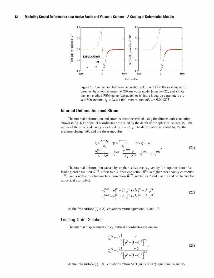
5. Diagram showing comparison between calculations of ground tilt in the east and north direction by a two-dimensional analytical model, and a finite element method numerical model ..........................................................................................................12
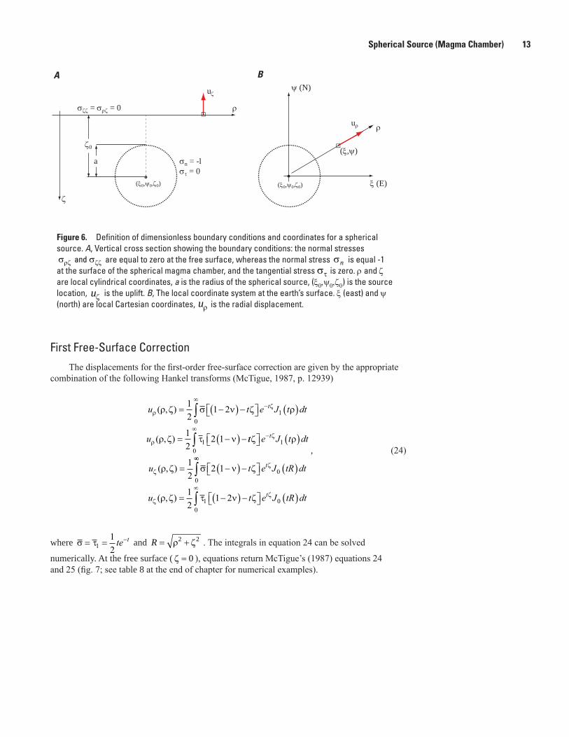
6. Diagram showing definition of dimensionless boundary conditions and coordinates for a spherical source ........................................................................................13
7. Graph showing first free-surface correction ........................................................................14 8. Graph showing higher order cavity correction at the free surface ..................................15 9. Graph showing sixth-order surface correction at 0ζ = .....................................................16 10. Graphs showing internal deformation caused by a spherical source ..............................17 11. Graphs showing internal strain caused by a spherical source ..........................................18

vi
Figures 12. Diagrams showing definition of coordinates system and boundary-value
problem for a spheroidal source ..............................................................................................20 13. Flow chart for coding Yang and others’ (1988) expressions for displacement, tilt,
and strain ....................................................................................................................................20 14. Graphs showing free-surface deformation caused by the inflation of a vertical
prolate spheroid ( φ = °0 ) for different values of the geometric aspect ratio A ...............25 15. Graphs showing free-surface deformation caused by the inflation of a tilted
( θ unequal to 0) and rotated (φ unequal to 0) prolate spheroid .....................................26 16. Graphs showing internal deformation caused by the inflation of a tilted and
rotated prolate spheroid ............................................................................................................27 17. Graph showing verification of the empirical correction for the volume change
of a pressurized prolate spheroid ............................................................................................28 18. Graphs showing ground tilt caused by the inflation of a tilted and rotated prolate
spheroid ........................................................................................................................................29 19. Graph showing internal strain caused by the inflation of a tilted and rotated
prolate spheroid ..........................................................................................................................30 20. Graph showing definition of boundary conditions and geometry for a sill-like
source ..........................................................................................................................................33 21. Graph showing matlab function fialko01.m flow chart for calculating and coding
the parameters for a sill-like source .......................................................................................33 22. Graphs showing surface deformation due to the inflation of a sill-like source;
internal deformation ...................................................................................................................34 23. Graph showing volume change for a sill-like source ..........................................................35 24. Graphs showing ground tilt caused by the inflation of a sill-like source ..........................35 25. Graphs showing internal strain caused by the inflation of a sill-like source ...................36 26. Program flow chart for rectangular dislocations .................................................................37 27. Diagrams showing Geometry of the dislocation model in a Cartesian coordinate
system; Geometry of the source model .................................................................................37 28. Vector and profile plots of the displacement field of a strike-slip
fault ..............................................................................................................................................44 29. Vector and profile plots of the displacement field of a dip-slip
fault ..............................................................................................................................................45 30. Vector and profile plots of the displacement field of a
tensile crack ................................................................................................................................46 31. Profile plots showing tilt caused by a tensile crack .............................................................47 32. Program flow chart for rectangular dislocations ..................................................................49 33. Vector and profile plots showing displacement fieldand straincaused by a
strike-slip fault ............................................................................................................................65 34. Graphs showing vector and profile plots of the displacement field and strain
caused by a dip-slip fault .........................................................................................................67 35. Graphs showing vector and profile plots of the displacement field and strain
caused by a tensile crack .........................................................................................................69 36. Graph showing representation of the fault geometry by segments, subsegments,
and tiles ........................................................................................................................................71 37. The Matlab script for coding a discretized fault includes four major steps .....................72 38. Diagrams showing segment, subsegment, and tile geometry ............................................74
vii
Figures—Continued 39. Graphs showing fault geometry and vector plot and profile plots of the
surface displacement caused by a right-lateral strike-slip fault ........................................76 40. Graphs showing fault geometry and vector plot and profile plots of the surface
displacement caused by a reverse dip-slip fault ..................................................................77 41. Graphs showing fault geometry and vector plot and profile plots of the surface
displacement caused by the opening of a tensile crack .....................................................78 42. Image showing grid and tile geometry for smoothing matrix D .........................................80 43. Grid used to compute the second-order finite-difference operator D; fault divied into
P=2 rows, N=9 columns, and 18 tiles of different width; smoothing operator D for the fault in B. ......................................................................................................................................81
44. Graph showing fault geometry used to validate the algorithm for the smoothing operator D ....................................................................................................................................84
45. Color maps for the smoothing operator, slip distribution, and finite difference second derivative 2∇ s for the fault geometry shown in figure 44 .......................................85
46. Graph showing fault geometry employed in the example ...................................................86
Tables 1. List of earthquake and volcano deformation sources described in this report .................2 2. The 14 transformation parameters between ITRF05 and ITRF00 .........................................4 3. Comparison of IRTF00 and IRTF05 parameters from itrf052itrf00.m with results from
the National Geodetic Survey code HTDP for epochs 2000 and 2010 ................................4 4. Comparison of Matlab function xyz2llh.m with NGS code HTDP ........................................5 5. Comparison of coordinates for the International Global Survey site FLIN computed
in the UTM system in ArcGIS and ll2utm.m (datum WGS 84) ...............................................7 6. Conversion of coordinates of GPS sites near the Augustine volcano from IRTF
to ENU .............................................................................................................................................8 7. Surface deformation, tilt, and internal deformation .............................................................19 8. Corrections for internal deformation ......................................................................................19 9. Internal deformation and strain ...............................................................................................19 10. General parameters ...................................................................................................................24 11. Surface deformation and ground tilt .......................................................................................30 12. Internal deformation and strain ................................................................................................30 13. Surface deformation and tilt .....................................................................................................36 14. Internal deformation and strain ...............................................................................................36 15. Strike-slip fault ...........................................................................................................................48 16. Dip-slip fault .................................................................................................................................48 17. Tensile crack ..............................................................................................................................48 18. Strike-slip fault (internal deformation and strain; function fA) ..........................................58 19. Dip-slip fault (internal deformation and strain; function fA) ...............................................58 20. Tensile crack (internal deformation and strain; function fA) ..............................................59 21. Scaling used to compute the dimensional displacement (function fA) ............................59 22. Strike-slip fault (internal deformation and strain; function fB) ..........................................60 23. Dip-slip fault (internal deformation and strain; function fB ) ..............................................60 24. Tensile crack (internal deformation and strain; function fB) .............................................61 25. Scaling (internal deformation and strain; function fB) ........................................................61
viii
Acronyms
EDM Electronic Distance MeterENU local east-north-up Cartesian coordinate systemFEM Finite Element MethodGPS Global Positioning SystemGTSM Gladwin Tensor StrainmetersInSAR Interferometric synthetic aperture radarITRF International Terrestrial Reference FrameLLH Latitude, longitude, heightLL Latitude, longitudePBO Plate Boundary ObservatoryUTM Universal Transverse MercatorWGS 84 World Geodetic System 1984
Tables—Continued
26. Strike-slip fault (internal deformation and strain; function fC) .........................................62 27. Dip-slip fault (internal deformation and strain; function fC) ..............................................63 28. Tensile crack (internal deformation and strain; function fC) ..............................................64 29. Scaling (internal deformation and strain; function fC) ........................................................64 30. Internal deformation and strain around a strike-slip fault ...................................................66 31. Internal deformation and strain around a dip-slip fault ......................................................68 32. Internal deformation and strain around a tensile crack. ....................................................70 33. Parameters for strike-slip fault segments .............................................................................76 34. Parameters for dip-slip fault segments...................................................................................77 35. Parameters for tensile-crack fault segments ........................................................................78 36. Values of fault parameters .......................................................................................................85 37. Values of fault parameters ........................................................................................................86 38. Values of the smoothing operator D .......................................................................................87 39. Values of the slip vector U ........................................................................................................87 40. Values of the product DU .........................................................................................................87 41. Values of the finite-difference second derivative 2∇ s ........................................................87
Introduction 1
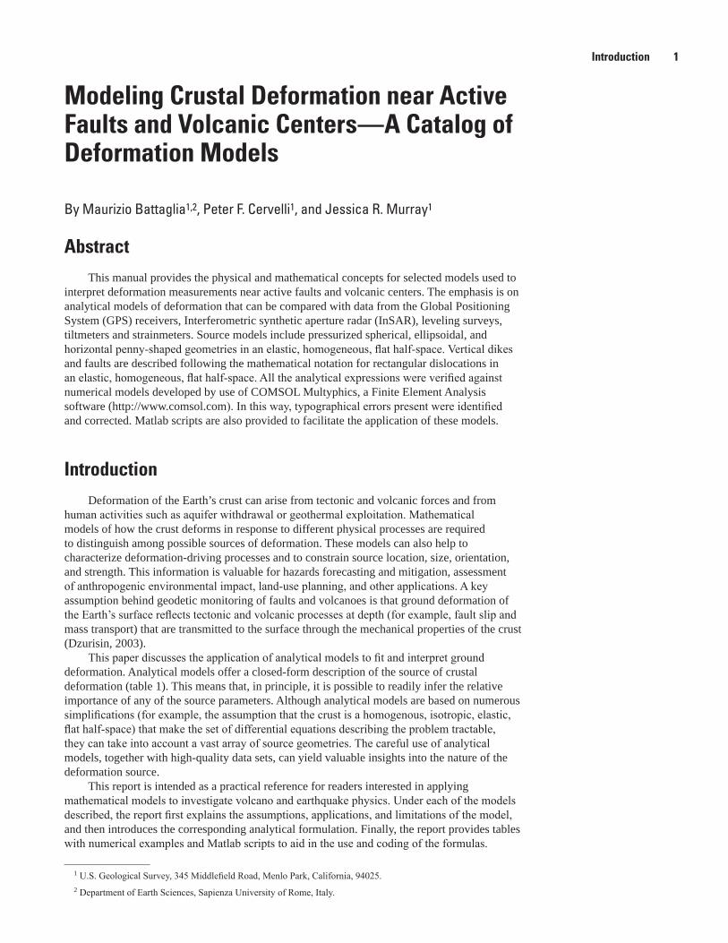
AbstractThis manual provides the physical and mathematical concepts for selected models used to
interpret deformation measurements near active faults and volcanic centers. The emphasis is on analytical models of deformation that can be compared with data from the Global Positioning System (GPS) receivers, Interferometric synthetic aperture radar (InSAR), leveling surveys, tiltmeters and strainmeters. Source models include pressurized spherical, ellipsoidal, and horizontal penny-shaped geometries in an elastic, homogeneous, flat half-space. Vertical dikes and faults are described following the mathematical notation for rectangular dislocations in an elastic, homogeneous, flat half-space. All the analytical expressions were verified against numerical models developed by use of COMSOL Multyphics, a Finite Element Analysis software (http://www.comsol.com). In this way, typographical errors present were identified and corrected. Matlab scripts are also provided to facilitate the application of these models.
IntroductionDeformation of the Earth’s crust can arise from tectonic and volcanic forces and from
human activities such as aquifer withdrawal or geothermal exploitation. Mathematical models of how the crust deforms in response to different physical processes are required to distinguish among possible sources of deformation. These models can also help to characterize deformation-driving processes and to constrain source location, size, orientation, and strength. This information is valuable for hazards forecasting and mitigation, assessment of anthropogenic environmental impact, land-use planning, and other applications. A key assumption behind geodetic monitoring of faults and volcanoes is that ground deformation of the Earth’s surface reflects tectonic and volcanic processes at depth (for example, fault slip and mass transport) that are transmitted to the surface through the mechanical properties of the crust (Dzurisin, 2003).
This paper discusses the application of analytical models to fit and interpret ground deformation. Analytical models offer a closed-form description of the source of crustal deformation (table 1). This means that, in principle, it is possible to readily infer the relative importance of any of the source parameters. Although analytical models are based on numerous simplifications (for example, the assumption that the crust is a homogenous, isotropic, elastic, flat half-space) that make the set of differential equations describing the problem tractable, they can take into account a vast array of source geometries. The careful use of analytical models, together with high-quality data sets, can yield valuable insights into the nature of the deformation source.
This report is intended as a practical reference for readers interested in applying mathematical models to investigate volcano and earthquake physics. Under each of the models described, the report first explains the assumptions, applications, and limitations of the model, and then introduces the corresponding analytical formulation. Finally, the report provides tables with numerical examples and Matlab scripts to aid in the use and coding of the formulas.
Modeling Crustal Deformation near Active Faults and Volcanic Centers—A Catalog of Deformation Models
By Maurizio Battaglia1,2, Peter F. Cervelli1, and Jessica R. Murray1
1 U.S. Geological Survey, 345 Middlefield Road, Menlo Park, California, 94025.2 Department of Earth Sciences, Sapienza University of Rome, Italy.
2 Modeling Crustal Deformation near Active Faults and Volcanic Centers—A Catalog of Deformation Models
A zipped file with MATLAB scripts can be downloaded from pubs.usgs.gov/tm/13/b1. The scripts are organized in folders, with each folder corresponding to a chapter in this publication (for example, the folder named “Geodetic transformations” contains MATLAB scripts for the geodetic transformation discuss in the section “Geodetic transformations” of this report). Folders may include subfolders with results from COULOMB 3.3 (“coulomb”) and Finite Element Method models (“FEM”), scripts verifying the algorithms (“verification”) and MATLAB functions (“functions”). The zipped file includes MATLAB functions for all the sources discussed in this publication and examples of the inversion of Global Positioning System (GPS) data for a spherical, spheroidal and sill-like source (the MATLAB Optimization Toolbox is required to run these examples). Online help can be obtained for each MATLAB function by typing “nameofthefunction help” in the MATLAB command line.
This publication is also designed to allow the user to turn directly to the desired model without reading any other sections (although a general understanding of the concepts and calculus behind the models from other literature will could enhance user experience, see for example Segall, 2010). As a result, some repetitions will be apparent if the manual is read sequentially. Many of the models described in this publication were taken from other credited or standard sources, but the authors themselves derived or rearranged many equations for this publication. All formulas have been checked for possible errors and verified against numerical models (COULOMB 3.3; http://earthquake.usgs.gov/research/modeling/coulomb/; FEM models). Since our emphasis is on describing the characteristics of the models and how they are used, the reader interested in the derivation and calculus of original equations is referred to the original literature. To limit the number of typographical errors, the formulas have been edited directly from the corresponding Matlab functions by using Mathtype.
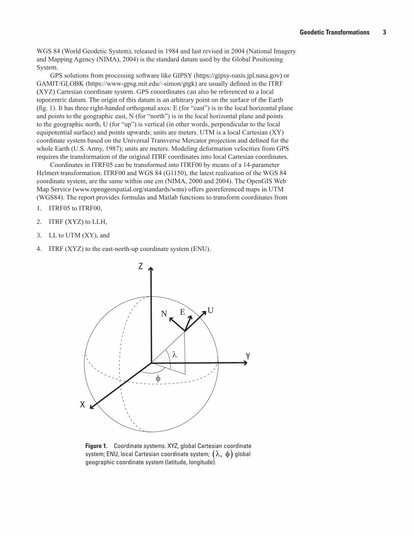
Geodetic TransformationsCoordinates can be expressed in systems defined by various datums, all of which are
related to each other through geometrical transformations. Geodetic datums describe the size and shape of the Earth, and the origin, orientation, and time derivatives of the coordinate system (fig. 1). The list below includes four common coordinate systems:1. global Cartesian (XYZ) system—International Terrestrial Reference Frame 2005 (ITRF05;
http://itrf.ensg.ign.fr); units are in meters.
2. global geographic system, either latitude, longitude, height (LLH) or latitude, longitude (LL)—International Terrestrial Reference Frame 2000 (ITRF00–WGS 84 ellipsoid; http://itrf.ensg.ign.fr); units are in degrees for latitude and longitude, and in meters for height.
3. local east-north-up (ENU) Cartesian coordinate system; units are in meters.
4. local Cartesian (XY) system—Universal Transverse Mercator coordinate system (UTM–WGS 84 ellipsoid); units are in meters.
Table 1. List of earthquake and volcano deformation sources described in this report.
Model Source Reference
Volcano source
Sphere Magma chamber McTigue (1987)Spheroid Conduit Yang and others (1988)Pennyshaped crack Sill Fialko and others (2001)Tensile dislocation Dike Okada (1985), Okada (1992)
Earthquake source
Rectangular dislocation Dip- and strike-slip fault (single rectangular segment)
Okada (1985), Okada (1992)
Superposition of rectangular segments
Fault composed of several rectangular segments
Jonsson and others (2002)
Geodetic Transformations 3
men12-7629_fig01
λ
φ
Z
N E U
Y
X
Figure 1. Coordinate systems. XYZ, global Cartesian coordinate system; ENU, local Cartesian coordinate system; λ φ, ( ) global geographic coordinate system (latitude, longitude).
WGS 84 (World Geodetic System), released in 1984 and last revised in 2004 (National Imagery and Mapping Agency (NIMA), 2004) is the standard datum used by the Global Positioning System.
GPS solutions from processing software like GIPSY (https://gipsy-oasis.jpl.nasa.gov) or GAMIT/GLOBK (https://www-gpsg.mit.edu/~simon/gtgk) are usually defined in the ITRF (XYZ) Cartesian coordinate system. GPS cooordinates can also be referenced to a local topocentric datum. The origin of this datum is an arbitrary point on the surface of the Earth (fig. 1). It has three right-handed orthogonal axes: E (for “east”) is in the local horizontal plane and points to the geographic east, N (for “north”) is in the local horizontal plane and points to the geographic north, U (for “up”) is vertical (in other words, perpendicular to the local equipotential surface) and points upwards; units are meters. UTM is a local Cartesian (XY) coordinate system based on the Universal Transverse Mercator projection and defined for the whole Earth (U.S. Army, 1987); units are meters. Modeling deformation velocities from GPS requires the transformation of the original ITRF coordinates into local Cartesian coordinates.
Coordinates in ITRF05 can be transformed into ITRF00 by means of a 14-parameter Helmert transformation. ITRF00 and WGS 84 (G1150), the latest realization of the WGS 84 coordinate system, are the same within one cm (NIMA, 2000 and 2004). The OpenGIS Web Map Service (www.opengeospatial.org/standards/wms) offers georeferenced maps in UTM (WGS84). The report provides formulas and Matlab functions to transform coordinates from 1. ITRF05 to ITRF00,
2. ITRF (XYZ) to LLH,
3. LL to UTM (XY), and
4. ITRF (XYZ) to the east-north-up coordinate system (ENU).
4 Modeling Crustal Deformation near Active Faults and Volcanic Centers—A Catalog of Deformation Models
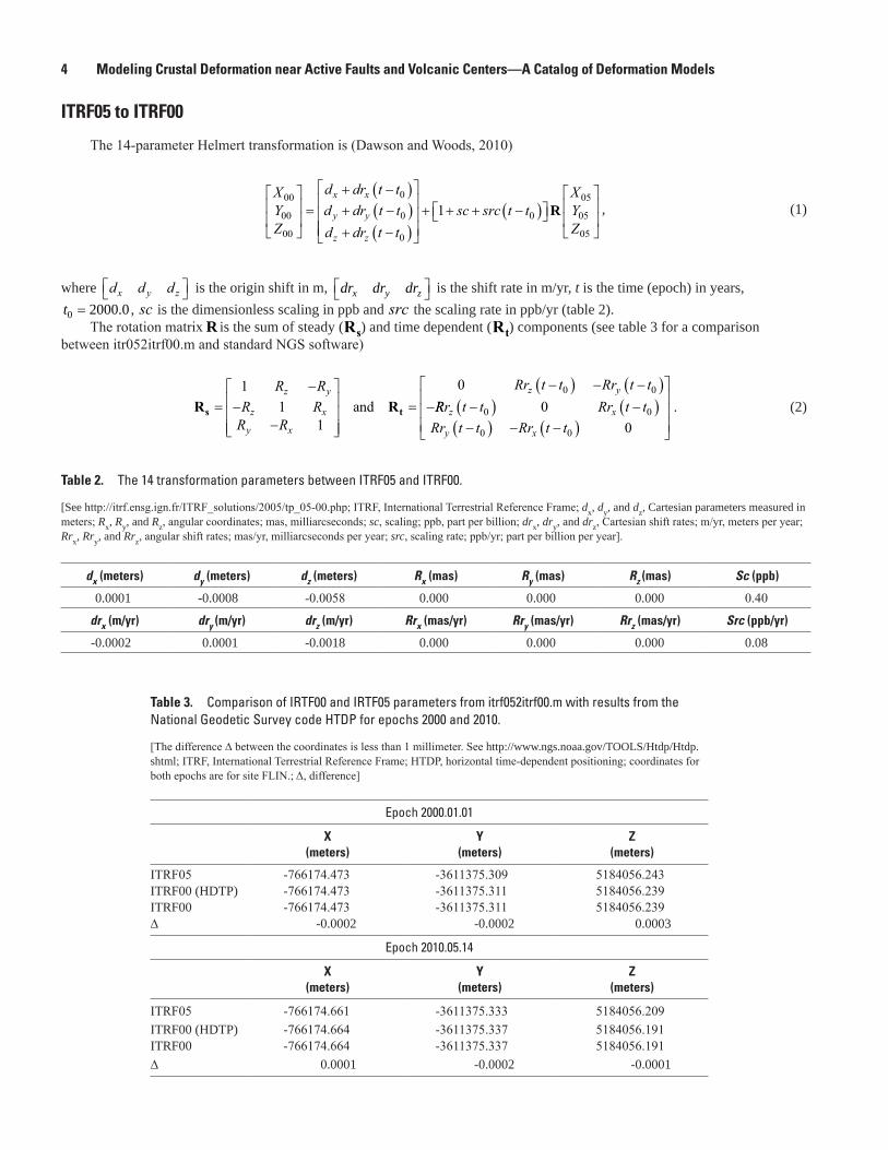
ITRF05 to ITRF00
The 14-parameter Helmert transformation is (Dawson and Woods, 2010)
XYZ
d dr t td dr t td dr t t
x x
y y
z z
00
00
00
0
0
0
=
+ −( )+ −( )+ −( )
+ + + −( )
1 0
05
05
05
sc src t tXYZ
R , (1)
where d d dx y z is the origin shift in m, x y zdr dr dr is the shift rate in m/yr, t is the time (epoch) in years,
0 2000.0t = , sc is the dimensionless scaling in ppb and src the scaling rate in ppb/yr (table 2).The rotation matrix R is the sum of steady (Rs) and time dependent (Rt) components (see table 3 for a comparison
between itr052itrf00.m and standard NGS software)
R Rs t=−
−−
=−( ) − −( )
−1
11
0 0 0R RR RR R
Rr t t Rr t tz y
z x
y x
z y
and RRr t t Rr t tRr t t Rr t t
z x
y x
−( ) −( )−( ) − −( )
0 0
0 0
00
. (2)
Table 3. Comparison of IRTF00 and IRTF05 parameters from itrf052itrf00.m with results from the National Geodetic Survey code HTDP for epochs 2000 and 2010.
[The difference ∆ between the coordinates is less than 1 millimeter. See http://www.ngs.noaa.gov/TOOLS/Htdp/Htdp.shtml; ITRF, International Terrestrial Reference Frame; HTDP, horizontal time-dependent positioning; coordinates for both epochs are for site FLIN.; Δ, difference]
Epoch 2000.01.01
X (meters)
Y (meters)
Z (meters)
ITRF05 -766174.473 -3611375.309 5184056.243ITRF00 (HDTP) -766174.473 -3611375.311 5184056.239ITRF00 -766174.473 -3611375.311 5184056.239∆ -0.0002 -0.0002 0.0003
Epoch 2010.05.14
X (meters)
Y (meters)
Z (meters)
ITRF05 -766174.661 -3611375.333 5184056.209ITRF00 (HDTP) -766174.664 -3611375.337 5184056.191ITRF00 -766174.664 -3611375.337 5184056.191∆ 0.0001 -0.0002 -0.0001
Table 2. The 14 transformation parameters between ITRF05 and ITRF00.
[See http://itrf.ensg.ign.fr/ITRF_solutions/2005/tp_05-00.php; ITRF, International Terrestrial Reference Frame; dx, dy, and dz, Cartesian parameters measured in meters; Rx, Ry, and Rz, angular coordinates; mas, milliarcseconds; sc, scaling; ppb, part per billion; drx, dry, and drz, Cartesian shift rates; m/yr, meters per year; Rrx, Rry, and Rrz, angular shift rates; mas/yr, milliarcseconds per year; src, scaling rate; ppb/yr; part per billion per year].
dx (meters) dy (meters) dz (meters) Rx (mas) Ry (mas) Rz (mas) Sc (ppb)
0.0001 -0.0008 -0.0058 0.000 0.000 0.000 0.40
drx (m/yr) dry (m/yr) drz (m/yr) Rrx (mas/yr) Rry (mas/yr) Rrz (mas/yr) Src (ppb/yr)
-0.0002 0.0001 -0.0018 0.000 0.000 0.000 0.08
Geodetic Transformations 5
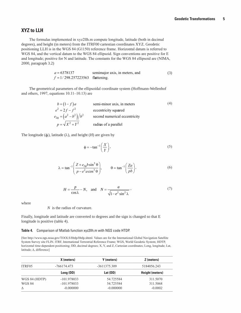
XYZ to LLH
The formulas implemented in xyz2llh.m compute longitude, latitude (both in decimal degrees), and height (in meters) from the ITRF00 cartestian coordinates XYZ. Geodetic positioning LLH is in the WGS 84 (G1150) reference frame. Horizontal datum is referred to WGS 84, and the vertical datum to the WGS 84 ellipsoid. Sign conventions are positive for E and longitude; positive for N and latitude. The constants for the WGS 84 ellipsoid are (NIMA, 2000, paragraph 3.2) a
f==
63781371 298 257223563
semimajor axis, in meters, andfl/ . aattening.
(3)
The geometrical parameters of the ellipsoidal coordinate system (Hoffmann-Wellenhof and others, 1997, equations 10.11–10.13) are b f a
e f f= −( )= −
122 2
semi-minor axis, in meterseccentricity squaaredsecond numerical eccentricity
radi
e a b b
p YX
22 2 2
2 2
φ = −
= +
( )uus of a parallel
(4)
The longitude (φ), latitude (λ), and height (H) are given by
φ = −
−tan 1 XY
, (5)
λθ
θθφ=
=
+
−− −tan , tan
sin
cos1 12
3
2 3
Z e b
p e aZapb
, (6)
2 2
, and1 incos s
apH N Ne
= −λ
=− λ
, (7)
where N is the radius of curvature.
Finally, longitude and latitude are converted to degrees and the sign is changed so that E longitude is positive (table 4).
Table 4. Comparison of Matlab function xyz2llh.m with NGS code HTDP.
[See http://www.ngs.noaa.gov/TOOLS/Htdp/Htdp.shtml. Values are for the International Global Navigation Satellite System Survey site FLIN. ITRF, International Terrestrial Reference Frame; WGS, World Geodetic System; HDTP, horizontal time-dependent positioning; DD, decimal degrees; X, Y, and Z, Cartesian coordinates; Long, longitude; Lat, latitude; Δ, difference]
X (meters) Y (meters) Z (meters)
ITRF05 -766174.473 -3611375.309 5184056.243
Long (DD) Lat (DD) Height (meters)
WGS 84 (HDTP) -101.978033 54.725584 311.5070WGS 84 -101.978033 54.725584 311.5068∆ -0.000000 -0.000000 -0.0002
6 Modeling Crustal Deformation near Active Faults and Volcanic Centers—A Catalog of Deformation Models
LL to UTM
The Matlab function ll2utm.m computes the E (east, meters) and N (north, meters) coordinates on the UTM grid from the WGS 84 (G1150) longitude (φ) and latitude (λ). According to the Defense Mapping Agency (1989) report, “The computations (* * *) are accurate to the nearest 0.001 arc second for geographic coordinates and to the nearest 0.01 meter for grid coordinates”, where 0.001 arc second = 73 10−× decimal degrees = 94.848 10−× rad. The UTM horizontal datum is the WGS 84 ellipsoid, with sign convention positive for E longitude and positive for N latitude.
The first step is to set the constants for the WGS 84 ellipsoid (NIMA, 2000, paragraph 3.2):
af
==
63781371 298 257223563
semimajor axis, in meters, andfl/ . aattening.
(8)
and the WGS 84 ellipsoid parameters (Defense Mapping Agency, 1989, paragraph 2–2.1):
b f ae f f= −( )= −
122 2
semiminor axis, in meterseccentricity squarredsecond numerical eccentricitye a b b
v a
e
22 2 2
2 21
φ
φ
= −
=−
( )
sinrradius of curvature in the prime vertical
(9)
( ) ( )( ) ( )( ) ( )
( )( ) ( )
( ) ( ) ( ) ( )
2 3 4 5
2 3 4 5
2 3 4 5
3 4 5
4 5
2 1 5 4 81 64
3 / 2 7 8 55 64
15 /16 0.75
(35 / 48) 11 /16
315 / 512
sin 2 sin 4 sin 6 sin 8
fnf
A a n n n n n
B a n n n n n
C a n n n n
D a n n n
E a n n
S A B C D E
φ
φ
φ
φ
φ
φ φ φ φ φ
=− = − + − + −
= − + − + = − + −
= − +
= −
= φ − φ + φ − φ + φ
, (10)
where S is the meridional arc.
The UTM projection parameters (Defense Mapping Agency, 1989, paragraph 2–2.2) are the longitude measured with respect to the central meridian (λ0 ), the central scale factor k0 , false easting (FE), and false northing (FN):
0 0, 0.99960 or 10,000,000 500,000
kFN FE
∆λ = λ − λ == =
, (11)
where FN is 0 for the northern hemisphere and 10,000,000 for the southern hemisphere.

Geodetic Transformations 7
The following terms are used to calculate the general equations which follow in this section (Defense Mapping Agency, 1989, paragraph 2–2.3):
T SkT v kT T e e p
1 0
2 0
3 22 2
22
22
212 5 9 4
==
= ( ) − + +
sin coscos tan cosφ φ
φ φ φφ ccos4 φ( )
(12)
T T e e p4 24 2 4
22 2
2360 61 58 270 330= ( ) − + + −cos tan tan cos tan cosφ φ φ φ φφ22
22 4
23 6 2
22 4
24
445 324 680
88
φ
φ φ φ φφ φ φ
φ
(+ + − +
+
e e e
e
cos cos tan cos
coss tan cos tan cos
cos
8 223 6 2
24 8
5 26
600 192
20160
φ φ φ φ φ
φ
φ φ− − )= ( )
e e
T T 11385 3111 5432 4 6
6 0
− + −( )=
tan tan tancos
φ φ φ
φT v k
T T e
T T7 6
2 22
2
8 64 2
6 1
120 5 18
= ( ) − +( )= ( ) − +
cos tan cos
cos tan ta
φ φ φ
φ φ
φ
nn cos tan cos
cos cos
42
2 22
2
22 4
23 6
14 58
13 4 6
φ φ φ φ
φ φ
φ φ
φ φ
+ − +(+ + −
e e
e e 44 24
5040 61 479
222 4 2
23 6
9 66
tan cos tan cos
cos ta
φ φ φ φ
φ
φ φe e
T T
− )= ( ) − nn tan tan2 4 6179φ φ φ+ −( )
The general formulas for the conversion of geographic coordinates to north (N) and east (E) grid coordinates (Defense Mapping Agency, 1989, paragraph 2–5; table 5) are
N FN T T T T TE FE T T T T= + + + + += + + + +
1 22
34
46
58
6 73
85
97
∆ ∆ ∆ ∆∆ ∆ ∆ ∆
λ λ λ λλ λ λ λ
(13)
Table 5. Comparison of coordinates for the International Global Survey site FLIN computed in the UTM system in ArcGIS and ll2utm.m (datum WGS 84).
[WGS, World Geodetic System; UTM, Universal Transverse Mercator; GIS, geographic information system; DD, decimal degrees; X, Y, and Z, global Cartesian coordinates; Long, longitude; Lat, latitude; Δ, difference]
Long (DD) Lat (DD)
WGS 84 (G1150) -101.9780327 54.7255844
E (meters) N (meters)
UTM (ArcGIS) 308230.414 6068325.668UTM 308230.413 6068325.666∆ -0.001 -0.002
8 Modeling Crustal Deformation near Active Faults and Volcanic Centers—A Catalog of Deformation Models
Local Coordinates (ENU)
XYZ to ENUThe Matlab function xyz2enu.m transforms global Cartestian coordinates (XYZ) into local
east-north-up (ENU) Cartesian coordinates. The origin of the local coordinate system is set to the minimum value of the (XYZ) coordinates. The transformation comprises two steps:1. Transform the origin from XYZ coordinates ( )0 0 0, , X Y Z to LL coordinates ( )0 0, φ λ , and
2. Convert XYZ coordinates to ENU (Hoffmann-Wellenhof and others, 1997, p. 149) through the equation
ENU
=
−− −
sin cossin cos sin sin cos
cos co
λ λφ λ φ λ φφ
0 0
0 0 0 0 0
0
0
ss cos sin sinλ φ λ φ0 0 0 0
0
0
0
−−−
X XY YZ Z
. (14)
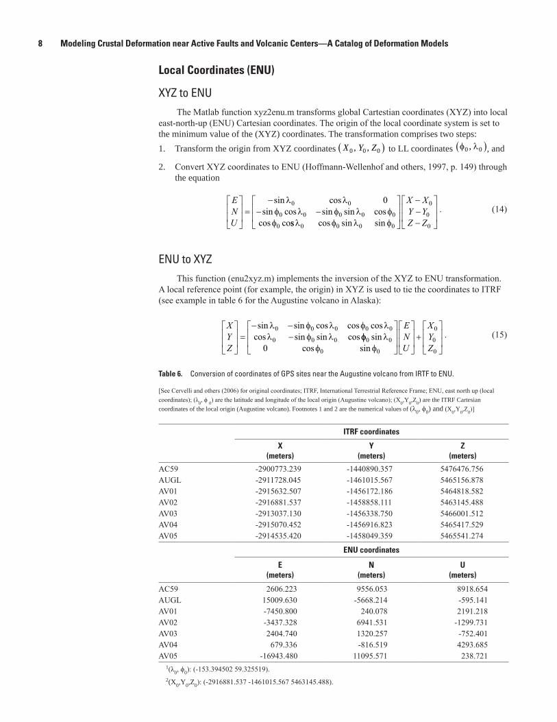
ENU to XYZThis function (enu2xyz.m) implements the inversion of the XYZ to ENU transformation.
A local reference point (for example, the origin) in XYZ is used to tie the coordinates to ITRF (see example in table 6 for the Augustine volcano in Alaska):
XYZ
=
− −−
sin sin cos cos coscos sin sin cos
λ φ λ φ λλ φ λ
0 0 0 0 0
0 0 0 φφ λφ φ
0 0
0 0
0
0
00sin
cos sin
+
ENU
XYZ
. (15)
Table 6. Conversion of coordinates of GPS sites near the Augustine volcano from IRTF to ENU.
[See Cervelli and others (2006) for original coordinates; ITRF, International Terrestrial Reference Frame; ENU, east north up (local coordinates); (λ0, ϕ 0) are the latitude and longitude of the local origin (Augustine volcano); (X0,Y0,Z0) are the ITRF Cartesian coordinates of the local origin (Augustine volcano). Footnotes 1 and 2 are the numerical values of (λ0, ϕ0) and (X0,Y0,Z0)]
ITRF coordinates
X (meters)
Y (meters)
Z (meters)
AC59 -2900773.239 -1440890.357 5476476.756AUGL -2911728.045 -1461015.567 5465156.878AV01 -2915632.507 -1456172.186 5464818.582AV02 -2916881.537 -1458858.111 5463145.488AV03 -2913037.130 -1456338.750 5466001.512AV04 -2915070.452 -1456916.823 5465417.529AV05 -2914535.420 -1458049.359 5465541.274
ENU coordinates
E (meters)
N (meters)
U (meters)
AC59 2606.223 9556.053 8918.654AUGL 15009.630 -5668.214 -595.141AV01 -7450.800 240.078 2191.218AV02 -3437.328 6941.531 -1299.731AV03 2404.740 1320.257 -752.401AV04 679.336 -816.519 4293.685AV05 -16943.480 11095.571 238.721
1(λ0, ϕ0): (-153.394502 59.325519).2(X0,Y0,Z0): (-2916881.537 -1461015.567 5463145.488).
Spherical Source (Magma Chamber) 9
Spherical Source (Magma Chamber)The deformation due to an expanding or contracting magma chamber has frequently been
modeled by a dilatation source in an elastic half space. The most commonly used is the Mogi, or point, source (Masterlark, 2007). The model simulates a small spherical source embedded in a homogeneous, isotropic, elastic, flat half-space (fig. 2).
The appeal of Mogi’s model lies in its combination of computational simplicity and remarkable ability to predict radially symmetric deformation caused by magma intrusion. The accuracy of an interpretation based on Mogi’s model, however, is subject to the suitability of the initial assumptions—an often overlooked consideration (Masterlark, 2007). For example, Mogi’s point-source model can explain stresses and displacements far away from the magma chamber, but the stresses are infinite at the source. In contrast, McTigue’s (1987) formulation provides an analytical solution with higher order terms that account for the finite shape of a spherical body. Thus, the local stresses at, and far from, the boundary of a chamber remain finite and can be calculated. McTigue’s results (1987) for vertical ( uz ) and radial ( ur) surface deformation caused by a pressurized ( P∆ ) spherical magma chamber of radius a and at position ( , , )x y z0 0 0 (fig. 2) can be written in the form
u Pa z
r z
azz = −( )
+( )−
+−( )
−−( )−
1 1 12 7 5
15 24 7
30
202 3 2
0
3
νµ
νν
ν∆55
02
202ν( ) +
zr z
, (16)
and
u Pa r
r z
azr = −( )
+( )−
+−( )
−−( )−
1 1 12 7 5
15 24 7 5
3
202 3 2
0
3
νµ
νν
ν∆νν( ) +
zr z
02
202
, (17)
where z0 is the depth of the source (a positive number), ν the Poisson’s ratio, and µ the shear modulus. A direct consequence of the assumption of a point source of dilatation is that the magma-chamber radius a and pressure change P∆ are inseparable because 3Pa∆ is the strength of the point singularity. This is why point source models typically calculate volume rather than pressure changes.
When the radius a is small relative to the depth z0 , so that ( )30a z is much less than
1, the Mogi assumptions are reasonable, and the McTigue (1987) correction is not needed. For example, when a z= 0 2 , the correction is only 12 percent, and it decreases to 3 percent for a z= 0 3 . This means that, if the overall accuracy of the geodetic survey is within 3–12 percent, the Mogi’s model is sufficient to fit the deformation. If the site effects induced by shallow heterogeneities and topography account for as little as 3–12 percent of the deformation signal, the Mogi’s model is again a good approximation.
We can use equations 16 and 17 and to compute the three components of surface deformation (for example, the components measured by GPS receivers) aligned to geographic east (x-axis), north (y-axis) and up (z-axis), as shown in figure 3 (see table 7 at the end of chapter for numerical examples).
u u u u xru yrux y z r r z =
. (18)

10 Modeling Crustal Deformation near Active Faults and Volcanic Centers—A Catalog of Deformation Models
men12-7629_fig03
−5000 0 5000−0.04
−0.03
−0.02
−0.01
0.00
0.01
0.02
0.03
0.04
X−di
spla
cem
ent,
in m
eter
s
−5000 0 5000
x, in meters−5000 0 5000
EXPLANATION
FEM
3D
2D
Figure 3. Free-surface deformation caused by a pressurized spherical magma chamber. Comparison between the three-dimensional (3D) semianalytical solution (equation 22), the two-dimensional (2D) analytical model (equations 16 and 17), and a numerical finite element method (FEM) model of the same source. The source is at the origin of the coordinate system, and its parameters are a = 500 meters, z a0 2 1 000= = , meters, and ∆P µ = 0 001273. .
Figure 2. Definition of boundary conditions and geometry for a spherical source (modified from McTigue, 1987). A, Vertical cross section showing he boundary conditions: the normal stresses σ σrz zz and are equal to zero at the free surface, whereas the normal stress σn is equal to the pressure change at the surface of the spherical magma chamber, and the tangential stress σt is zero. r and z are local cylindrical coordinates, a is the radius of the spherical source, (x0,y0,z0) is the source location, uz is the uplift. B, The local coordinate system at the earth’s surface. x (east) and y (north) are local Cartesian coordinates, ur is the radial displacement.
men12-7629_fig02
z0
a
z
rσzz = σrz = 0
σn = -∆Pσt = 0
uz
ur
y (N)
x (E)
(x,y)
r2 = (x-x0)2 + (y-y0)2
A B
§
� �
r
(x0,y0,z0)
§
(x0,y0,z0)
Spherical Source (Magma Chamber) 11
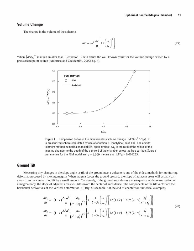
Volume Change
The change in the volume of the sphere is
∆∆V a P a
z= +
πµ
3
0
4
1 . (19)
When a z04( ) is much smaller than 1, equation 19 will return the well known result for the volume change caused by a
pressurized point source (Amoruso and Crescentini, 2009; fig. 4).
Figure 4. Comparison between the dimensionless volume change ( ∆ ∆V a P( )π µ3 ) of a pressurized sphere calculated by use of equation 19 (analytical, solid line) and a finite element method numerical model (FEM, open circles). a/z0 is the ratio of the radius of the magma chamber to the depth of the centroid of the chamber below the free surface. Source parameters for the FEM model are a = 1 000, meters and ∆P µ = 0 001273. .
men12-7629_fig04
a/z0
∆V/(π
a3∆P
/µ)
0.95
1.00
1.05
1.10
1.15
1.20
0.0 0.2 0.4 0.6 0.8
EXPLANATION
FEM
Analytical
Ground Tilt
Measuring tiny changes in the slope angle or tilt of the ground near a volcano is one of the oldest methods for monitoring deformation caused by moving magma. When magma forces the ground upward, the slope of adjacent areas will usually tilt away from the center of uplift by a small amount. Conversely, if the ground subsides as a consequence of depressurization of a magma body, the slope of adjacent areas will tilt toward the center of subsidence. The components of the tilt vector are the horizontal derivatives of the vertical deformation uz (fig. 5; see table 7 at the end of chapter for numerical example).
dudx
Pa xz
r z
az
z = − −( )+( )
−−
+( ) −1 3 1
7 51 5 1 18
30
202 5 2
0
3
νµ ν
ν∆ . ..75 2
1
02
202
30
2
−( )+
= − −( )
ν
νµ
zr z
dudy
Pa yz
rz ∆
++( )−
−
+( ) − −( )
+
z
az
zr z
02 5 2
0
302
2023 1
7 51 5 1 18 75 2
νν ν. .
. (20)
12 Modeling Crustal Deformation near Active Faults and Volcanic Centers—A Catalog of Deformation Models
Internal Deformation and Strain
The internal deformation and strain is better described using the dimensionless notation shown in fig. 6.The spatial coordinates are scaled by the depth of the spherical source z0 . The radius of the spherical cavity is defined by ε = a z0 . The deformation is scaled by z0 , the pressure change P∆ , and the shear modulus µ
ξ ψ ρ ξ ψ
µ µζ ρ
=−
=−
= +
= =
x xz
y yz
uz P
u uz P
uzD
D rD
D
0
0
0
0
2 2
3
0
33
0
3( )
( )( )
(
∆ ∆)) ( )= ρ ζu
D3
, (21)
The internal deformation caused by a spherical source is given by the superposition of a leading-order solution u ( )0 , a first free-surface correction u ( )1 , a higher order cavity correction u ( )3 , and a sixth-order free-surface correction u ( )6 (see tables 7 and 9 at the end of chapter for numerical examples):
u u u u uu u u
D
Dρ ρ ρ ρ ρ
ζ ζ ζ
ε ε ε
ε ε
( ) ( ) ( ) ( ) ( )
( ) ( ) ( )
3 0 3 1 3 3 6 6
3 0 3 1
= + + +
= + + 33 3 6 6u uζ ζε( ) ( )+. (22)
At the free surface ( ζ = 0 ), equations return equations 16 and 17.
Leading-Order SolutionThe internal displacements in cylindrical coordinates system are
u
u
ρ
ζ
ερ
ρ ζ
εζ
ρ ζ
( )
( )
0 3
2 2 3 2
0 3
2 2 3 2
14 1
14
1
1
=+ −( )
=−
+ −( )
. (23)
At the free surface ( ζ = 0 ), equations return McTigue’s (1987) equations 14 and 15.
Figure 5. Comparison between calculations of ground tilt in the east and north direction by a two-dimensional (2D) analytical model (equation 20), and a finite element method (FEM) numerical model. As in figure 3, source parameters are a = 500 meters, z a0 2 1 000= = , meters, and ∆P µ = 0 001273. .
men12-7629_fig05
−5000 0 5000−1.0
−0.5
0.0
0.5
1.0
−1.0
−0.5
0.0
0.5
1.0
Tilt
(eas
t), in
radi
ans
x 10
-4
−5000 0 5000
X, in meters
Tilt
(nor
th),
in ra
dian
s x
10-4
FEM
2D
EXPLANATION
Spherical Source (Magma Chamber) 13
First Free-Surface CorrectionThe displacements for the first-order free-surface correction are given by the appropriate
combination of the following Hankel transforms (McTigue, 1987, p. 12939)
u t e J t dt
u
tρ
ζ
ρ
ρ ζ σ ν ζ ρ
ρ ζ τ ν
( , )
( , )
= −( ) − ( )
= −( ) −
−∞
∫12
1 2
12
2 1
10
1 tt e J t dt
u t e J tR dt
t
t
ζ ρ
ρ ζ σ ν ζ
ζ
ζζ
( )
= −( ) − ( )
−∞
∫ 10
00
12
2 1( , )∞∞
∞
∫
∫= −( ) − ( )u t e J tR dttζ
ζρ ζ τ ν ζ( , ) 12
1 21 00
, (24)
where σ τ= = −1
12te t and R = +ρ ζ2 2 . The integrals in equation 24 can be solved
numerically. At the free surface ( ζ = 0 ), equations return McTigue’s (1987) equations 24 and 25 (fig. 7; see table 8 at the end of chapter for numerical examples).
men12-7629_fig06
ζ0
a
ζ
ρσζζ = σρζ = 0
σn = -1στ = 0
uζ
uρ
ψ (N)
ξ (E)
(ξ,ψ)
A B
§
� �
ρ
(ξ0,ψ0,ζ0)
§
(ξ0,ψ0,ζ0)
Figure 6. Definition of dimensionless boundary conditions and coordinates for a spherical source. A, Vertical cross section showing the boundary conditions: the normal stresses σ σρζ ζζ and are equal to zero at the free surface, whereas the normal stress σn is equal -1 at the surface of the spherical magma chamber, and the tangential stress στ is zero. ρ and ζ are local cylindrical coordinates, a is the radius of the spherical source, (x0,y0,ζ0) is the source location, uζ is the uplift. B, The local coordinate system at the earth’s surface. x (east) and y (north) are local Cartesian coordinates, uρ is the radial displacement.
14 Modeling Crustal Deformation near Active Faults and Volcanic Centers—A Catalog of Deformation Models
Higher Order Cavity CorrectionThe displacements for the higher order cavity correction are given by
u u uu u u
R
R
ρ θ
ζ θ
θ θ
θ θ
( )
( )
sin cos
cos sin
3
3
= +
= −, (25)
where
sin ; cosθ
ρθ
ζ
ρ ζ
= =−
= + −( )R R
R
1
12 2. (26)
McTigue’s (1987) equations 38–41 provide these expressions for uR and uθ :
uDR
P CDR
PR
u C
R = − + −( ) −
= −
12
5 4 32
03
2 0 23 2
3
222
23
( )( )
( )
( )
ν
θ 11 2 12
123
2 22−( ) +
νθ
DR R
dPd
( )
, (27)
where the C and D coefficients are
C D D23 3
03 3
23 55 2
25 7 5112
24 7 5
( ) ( ) ( ),=−−( )
= −+
=−−( )
ενν
εν
ενν
and , (28)
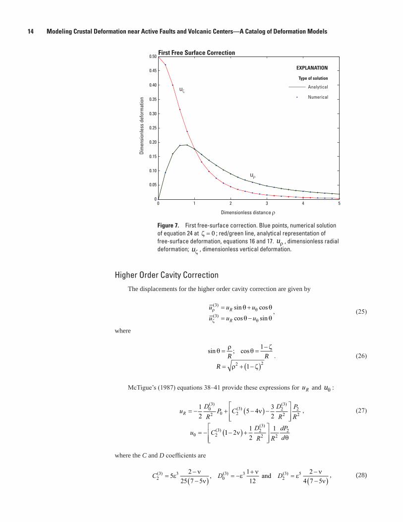
Figure 7. First free-surface correction. Blue points, numerical solution of equation 24 at ζ = 0 ; red/green line, analytical representation of free-surface deformation, equations 16 and 17. uρ , dimensionless radial deformation; uζ , dimensionless vertical deformation.
men12-7629_fig07
0 1 2 3 4 50
0.05
0.10
0.15
0.20
0.25
0.30
0.35
0.40
0.45
0.50First Free Surface Correction
Dimensionless distance ρ
Dim
ensi
onle
ss d
efor
mat
ion
Type of solution
uζ
uρ
Analytical
Numerical
EXPLANATION
Spherical Source (Magma Chamber) 15
and the Legendre’s polynomial and derivatives are
P P dPd0 2
2 21 12
3 1 3= = −( ) =, cos cosθθ
θ and . (29)
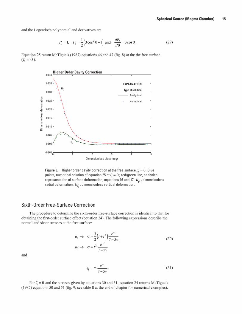
Equation 25 return McTigue’s (1987) equations 46 and 47 (fig. 8) at the the free surface(ζ = 0 ).
men12-7629_fig08
0 1 2 3 4 5−0.005
0.000
0.005
0.010
0.015
0.020
0.025
0.030
0.035
0.040Higher Order Cavity Correction
Dimensionless distance ρ
Dim
ensi
onle
ss d
efor
mat
ion
Type of solutionuζ
uρ
Analytical
Numerical
EXPLANATION
Figure 8. Higher order cavity correction at the free surface, 0ζ = . Blue points, numerical solution of equation 25 at 0ζ = ; red/green line, analytical representation of surface deformation, equations 16 and 17. uρ , dimensionless radial deformation; uζ , dimensionless vertical deformation.
Sixth-Order Free-Surface CorrectionThe procedure to determine the sixth-order free-surface correction is identical to that for
obtaining the first-order surface effect (equation 24). The following expressions describe the normal and shear stresses at the free surface:
u t t e
u t e
t
t
ρ
ζ
σν
σν
→ +( ) −
→−
−
−
32 7 5
7 5
2
2
, (30)
and
τν1
2
7 5 t e t−
−. (31)
For 0ζ = and the stresses given by equations 30 and 31, equation 24 returns McTigue’s (1987) equations 50 and 51 (fig. 9; see table 8 at the end of chapter for numerical examples).

16 Modeling Crustal Deformation near Active Faults and Volcanic Centers—A Catalog of Deformation Models
Internal DeformationFigure 10 on the next page shows the verification for the expression for internal
deformation (equation 22).
StrainStrainmeters can resolve changes in strain of less than one part per billion (1 mm in
1,000 km) over short periods, which makes them ideal for capturing transient deformation over time intervals ranging from seconds to months. Gladwin Tensor Strainmeters (GTSMs), the instruments used by the Plate Boundary Observatory (PBO), are designed to measure three components that describe the horizontal strain tensor: the areal strain εa, and shear strains γ1 and γ2 . Traditional engineering analysis has led to these quantitative definitions of quantities εa , γ1 , and γ2 :
ε ε ε γ ε ε γ ε
ε ε
a xx yy xx yy xy
xxx
yyyu
xuD D
= + = − =
=∂∂
=∂
, , ;
,( ) (
1 2 23 3
and )) ( ) ( )
, .∂
= =∂∂
+∂
∂
y
uy
uxxy yx
x yD D
and ε ε12
3 3 . (32)
Because of the complexity of the equation 22 for the internal deformation, we compute the strain components shown in equation 32 by use of numerical derivatives (see appendix 1).
Figure 9. Sixth-order surface correction at 0ζ = . Blue points, numerical solution (equations 24, 30, and 31) at 0ζ = ; red/green line, analytical representation of surface deformation, equations 16 and 17. uρ , dimensionless radial deformation; uζ , dimensionless vertical deformation.
men12-7629_fig09
0 1 2 3 4 5−0.1
0
0.1
0.2
0.3
0.4
0.5
0.6
0.7Sixth-order surface correction
Dimensionless distance ρ
Dim
ensi
onle
ss d
efor
mat
ion
Analytical
Numerical
Type of solutionuζ
uρ
EXPLANATION
Spherical Source (Magma Chamber) 17
men12-7629_fig10
−0.03
−0.02
−0.01
0.00 0.00
0.01
0.02
0.03
X, in meters
FEM
3D
−0.03
−0.02
−0.01
0.01
0.02
0.03
0
0.02
0.04
0.06
0.08
0.10
0.12
0.14
0.16
−5000 0 5000−0.05
0.00 0.00
0.05
X−di
spla
cem
ent,
in m
eter
s
−5000 0 5000−0.05
0.05Y−
disp
lace
men
t, in
met
ers
−5000 0 50000
0.05
0.10
0.15
0.02
0.25
0.03
0.35
Z−di
spla
cem
ent,
in m
eter
s
EXPLANATION
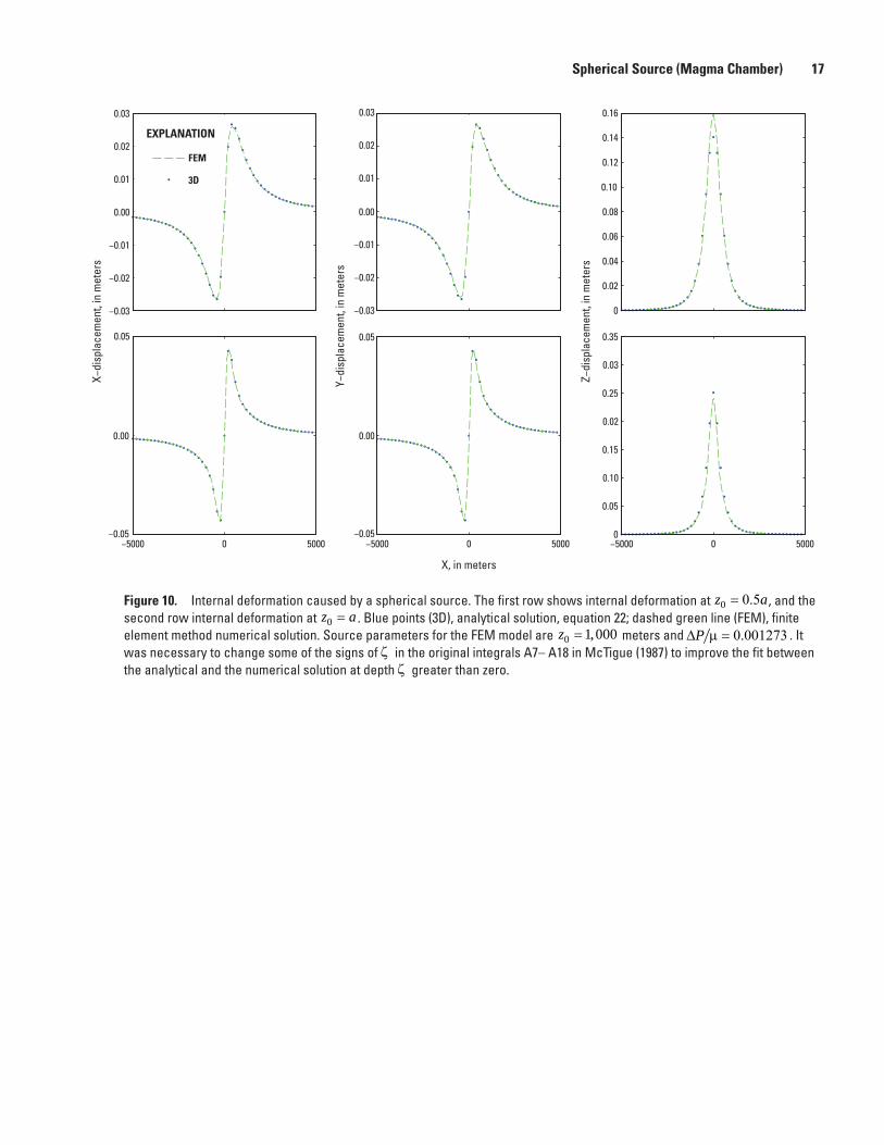
Figure 10. Internal deformation caused by a spherical source. The first row shows internal deformation at 0 0.5z a= , and the second row internal deformation at 0z a= . Blue points (3D), analytical solution, equation 22; dashed green line (FEM), finite element method numerical solution. Source parameters for the FEM model are 0 1,000z = meters and 0.001273P∆ µ = . It was necessary to change some of the signs of ζ in the original integrals A7– A18 in McTigue (1987) to improve the fit between the analytical and the numerical solution at depth ζ greater than zero.
18 Modeling Crustal Deformation near Active Faults and Volcanic Centers—A Catalog of Deformation Models
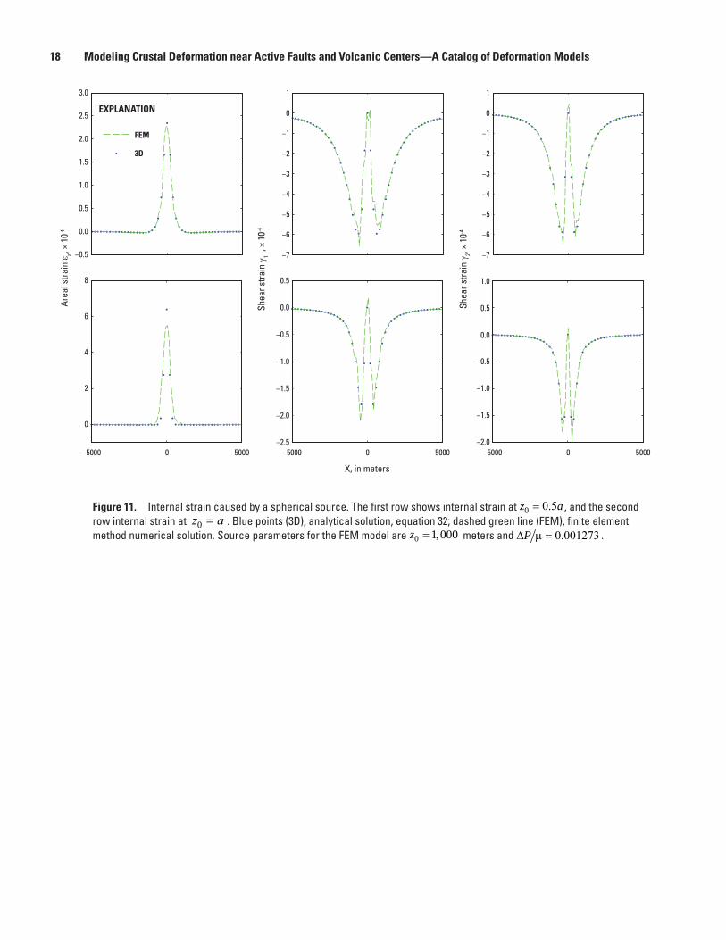
Figure 11. Internal strain caused by a spherical source. The first row shows internal strain at 0 0.5z a= , and the second row internal strain at z a0 = . Blue points (3D), analytical solution, equation 32; dashed green line (FEM), finite element method numerical solution. Source parameters for the FEM model are 0 1,000z = meters and 0.001273P∆ µ = .
men12-7629_fig11
−0.5
0.0
0.5
1.0
1.5
2.0
2.5
3.0
FEM
3D
−7
−6
−5
−4
−3
−2
−1
0
1
−7
−6
−5
−4
−3
−2
−1
0
1
X, in meters
Area
l stra
in ε a, ×
10-4
Shea
r stra
in γ
1 , ×
10-4
Shea
r stra
in γ
2, × 1
0-4
−5000 0 5000
0
2
4
6
8
−5000 0 5000−2.5
−2.0
−1.5
−1.0
−0.5
0.0
0.5
−5000 0 5000−2.0
−1.5
−1.0
−0.5
0.0
0.5
1.0
EXPLANATION
Spherical Source (Magma Chamber) 19
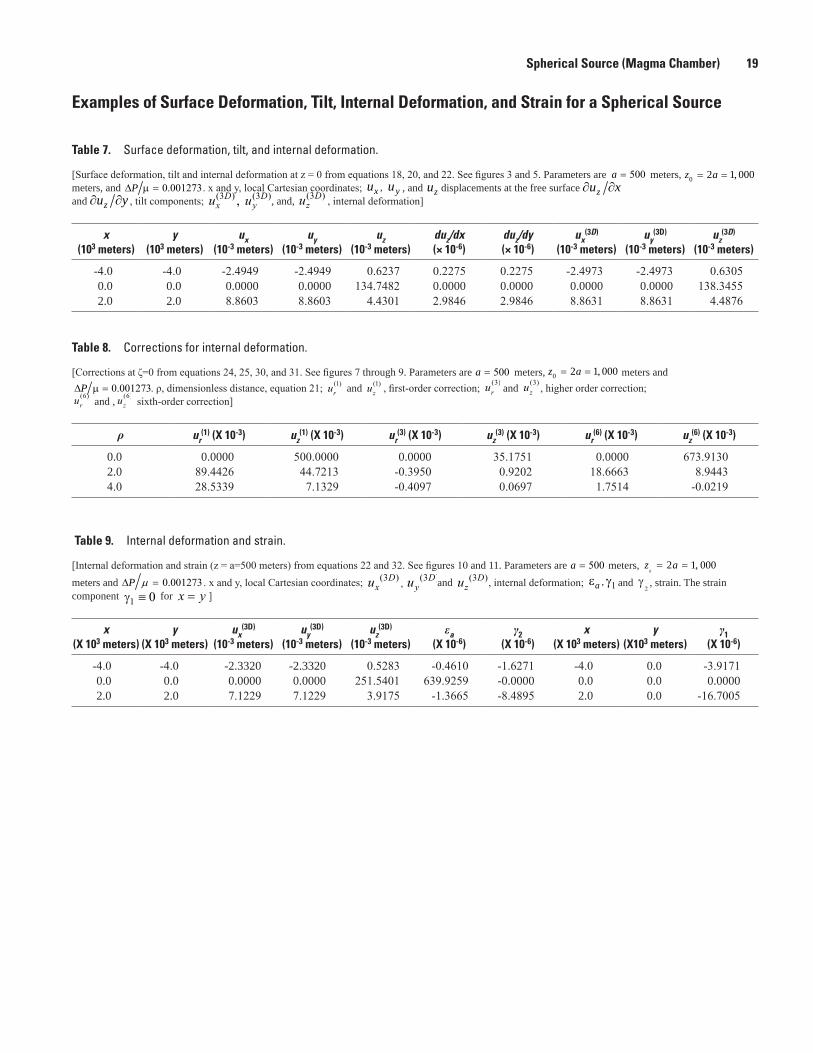
Table 7. Surface deformation, tilt, and internal deformation.
[Surface deformation, tilt and internal deformation at z = 0 from equations 18, 20, and 22. See figures 3 and 5. Parameters are 500a = meters, 0 2 1, 000z a= = meters, and 0.001273P∆ µ = . x and y, local Cartesian coordinates; , x yu u , and zu displacements at the free surface zu x∂ ∂ and zu y∂ ∂ , tilt components; u ux
DyD( ) ( ),3 3 , and, uz
D( )3 , internal deformation]
x (103 meters)
y (103 meters)
ux (10-3 meters)
uy (10-3 meters)
uz (10-3 meters)
duz/dx (× 10-6)
duz/dy (× 10-6)
ux(3D)
(10-3 meters)uy
(3D) (10-3 meters)
uz(3D)
(10-3 meters)
-4.0 -4.0 -2.4949 -2.4949 0.6237 0.2275 0.2275 -2.4973 -2.4973 0.63050.0 0.0 0.0000 0.0000 134.7482 0.0000 0.0000 0.0000 0.0000 138.34552.0 2.0 8.8603 8.8603 4.4301 2.9846 2.9846 8.8631 8.8631 4.4876
Table 8. Corrections for internal deformation.
[Corrections at ζ=0 from equations 24, 25, 30, and 31. See figures 7 through 9. Parameters are 500a = meters, 0 2 1, 000z a= = meters and∆P µ = 0 001273. . ρ, dimensionless distance, equation 21; ur
( )1 and uz( )1 , first-order correction; ur
( )3 and uz( )3 , higher order correction;
ur( )6 and , uz
( )6 sixth-order correction]
ρ ur(1) (X 10-3) uz
(1) (X 10-3) ur(3) (X 10-3) uz
(3) (X 10-3) ur(6) (X 10-3) uz
(6) (X 10-3)
0.0 0.0000 500.0000 0.0000 35.1751 0.0000 673.91302.0 89.4426 44.7213 -0.3950 0.9202 18.6663 8.94434.0 28.5339 7.1329 -0.4097 0.0697 1.7514 -0.0219
Table 9. Internal deformation and strain.
[Internal deformation and strain (z = a=500 meters) from equations 22 and 32. See figures 10 and 11. Parameters are 500a = meters, 0
2 1, 000z a= =
meters and 0.001273P∆ =µ . x and y, local Cartesian coordinates; u uxD
yD( ) , ( )3 3 and uz
D( )3 , internal deformation; ε γ1a , and γ2, strain. The strain
component γ1 0≡ for x y= ]
x (X 103 meters)
y(X 103 meters)
ux(3D)
(10-3 meters)uy
(3D)
(10-3 meters)uz
(3D)
(10-3 meters)εa
(X 10-6)γ2
(X 10-6)x
(X 103 meters)y
(X103 meters)γ1
(X 10-6)
-4.0 -4.0 -2.3320 -2.3320 0.5283 -0.4610 -1.6271 -4.0 0.0 -3.9171 0.0 0.0 0.0000 0.0000 251.5401 639.9259 -0.0000 0.0 0.0 0.0000 2.0 2.0 7.1229 7.1229 3.9175 -1.3665 -8.4895 2.0 0.0 -16.7005
Examples of Surface Deformation, Tilt, Internal Deformation, and Strain for a Spherical Source
20 Modeling Crustal Deformation near Active Faults and Volcanic Centers—A Catalog of Deformation Models
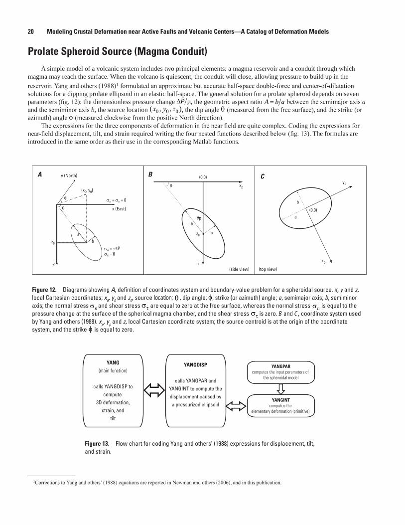
Prolate Spheroid Source (Magma Conduit)A simple model of a volcanic system includes two principal elements: a magma reservoir and a conduit through which
magma may reach the surface. When the volcano is quiescent, the conduit will close, allowing pressure to build up in the reservoir. Yang and others (1988)1 formulated an approximate but accurate half-space double-force and center-of-dilatation solutions for a dipping prolate ellipsoid in an elastic half-space. The general solution for a prolate spheroid depends on seven parameters (fig. 12): the dimensionless pressure change ∆P µ, the geometric aspect ratio A b a= between the semimajor axis a and the semiminor axis b, the source location ( , , )x y z0 0 0 , the dip angle θ (measured from the free surface), and the strike (or azimuth) angle φ (measured clockwise from the positive North direction).
The expressions for the three components of deformation in the near field are quite complex. Coding the expressions for near-field displacement, tilt, and strain required writing the four nested functions described below (fig. 13). The formulas are introduced in the same order as their use in the corresponding Matlab functions.
men12-7629_fig12
x (East)
y (North)
θ
φ
z
ba
(x0, y0)
σn = στ = 0
σn = -∆Pστ = 0
z0
yp
xp θ
z
b
a
z0
(0,0)
(side view)
BA
xp
yp
(0,0)a
b
(top view)
C
Figure 12. Diagrams showing A, definition of coordinates system and boundary-value problem for a spheroidal source. x, y and z, local Cartesian coordinates; x0, y0 and z0, source location; θ , dip angle; φ, strike (or azimuth) angle; a, semimajor axis; b, semiminor axis; the normal stress σn and shear stress στ are equal to zero at the free surface, whereas the normal stress σn is equal to the pressure change at the surface of the spherical magma chamber, and the shear stress στ is zero. B and C, coordinate system used by Yang and others (1988). xp, yp and z, local Cartesian coordinate system; the source centroid is at the origin of the coordinate system, and the strike φ is equal to zero.
men12-7629_fig13
YANG(main function)
calls YANGDISP tocompute
3D deformation,strain, and
tilt
YANGDISP
calls YANGPAR and YANGINT to compute the displacement caused by a pressurized ellipsoid
óYANGPAR
computes the input parameters of the spheroidal model
YANGINTcomputes the
elementary deformation (primitive) óò
Figure 13. Flow chart for coding Yang and others’ (1988) expressions for displacement, tilt, and strain.
1Corrections to Yang and others’ (1988) equations are reported in Newman and others (2006), and in this publication.
Prolate Spheroid Source (Magma Conduit) 21
Coordinates and Displacement (YANGDISP)To compute the displacement, coordinates must be transformed from the Cartesian
coordinate system (UTM) onto the coordinate system used by Yang and others (1988). The displacement vectors then can be back-transformed onto the original system (fig. 12).
We first translate and rotate the coordinates
x x x y yy x x y yp
p
= −( ) − −( )= −( ) + −( )
cos sinsin cos
φ φφ φ
0 0
0 0
, (33)
and then we compute the general expressions Up U c U c
Up U c U cUp U c U
x
y
z
= − = − = −= − = − = −= = +
1 1
2 2
3 3
( ) ( )( ) ( )( )
ξ ξξ ξξ (( )ξ = −c
(34)
for the displacement in Yang and others’ (1988) coordinate system, where * †
†0 1 1
1,2,3( , , , , , , , , , , , , )
i i i
i i p p
U U U iU U x y z z a b a b P
= + == θ x µ ν
(35)
are the primitive of the displacement for a prolate ellipsoid. The formulas for Ui* and †
iU are given by equations 49 and 50. Finally, the displacement vector Up is back-transformed onto the original coordinate system (see figs. 14 and 15 in the Verification section, p. 25):
u Up Upu Up Upu Up
x x y
y x y
z z
= ⋅ + ⋅= − ⋅ + ⋅=
cos sinsin cosφ φφ φ . (36)
Primitive (YANGINT)To compute the primitive *
iU and †iU , we must first introduce new coordinates and
parameters (see Yang and others, 1988, p. 4251): 2 3
1 2 3 0 3 0
1 1 2 2 2 3 3
2 2 2 2 2 21 1 2 3 2
3 3 3 3
2 2 3 2 2 3
3 2 3 3 2 3
3 3
1 2 3
3 3
cos sin
sin cos sin cos
cos sin cos sin
p px x x y x z z x z zy x y x y x y xr x x q
R y
x xr x x q x xr r
y y R y
q
y y
q
x = x θ x = x θ= = = − = += = − x = − x = + x= θ − θ = θ + θ
= θ + θ = − θ + θ= − x
= + + = + +
= + x
(37)
To make the formulas valid for dip angles θ unequal to 90 (in other words, a spheroid that is not vertical), we must correct the parameter C0 (see Yang and others, 1988, p. 4251, for the original expression):
0 0 sinC z= θ . (38)
22 Modeling Crustal Deformation near Active Faults and Volcanic Centers—A Catalog of Deformation Models
To prevent a “divide by zero” warning at the origin, we must add 150 1 10−ε = ⋅ at the
denominator in the formula for β
βθ θ
θ ε=
+ +( ) +( )+
q R qy
2 2 3
1 0
1cos sincos
. (39)
Additional parameters used to simplify the expressions for the deformation are
3 1 3 2 3 2 33 3
3 1 3 2 3 2 33 3ln( ) ln( ) ln( )dr R r dq R q dy R y
lr R r lq R q ly R y= + = + = +
= + = + = +, (40)
A a
R drb lr
rdr
A aR dq
b lqqdq
11
1 31 3
3
3
11
2 31 3
3
3
*
*
= + ++
= − − +−
ξ
ξ
, (41)
31 1 31 2
32 1 3 2 2 3 3
3 33 1 3 2
1 2
A lr A lqR R
A R r lr A R q lqr q
A R A RR R
x x= + = −
= − = −x x
= + = −
, and (42)
B a
Rb A a
Rb A
BC
R
*
= +
+ −( ) +
=+( )
−
1
11 2
1
21 2
0
2
2 3 4 2ν
ξ ξAA C lq2 0 3−
. (43)
The following four parameters F are called in *iU and †
iU (see equations 49 and 50). They were modified from the original formulation of Yang and others (1988) to improve the fit with the numerical FEM solution for internal deformation (fig. 16):
FFFF
1
2
1
2
00
00
*
*==
==
. (44)
Prolate Spheroid Source (Magma Conduit) 23
The parameters f also are called in *iU and †
iU (see equations 49 and 50). While the formulas for f1 and 2f are from Yang and others (1988), the equation for f3 was corrected by Newman and others (2006):
( )1
111 1 1 2 1 33 3 32
3
3 tansin 2 .* tan 2 4yf y ly y lq q y lq x
cosdy cos
−−x β
= + θ − + β + −θθ
. (45)
f y
dyq lq q ly y R y2
2
32 2 3 2 3 1
12 3
3 2= + − + + −( )( −ξ
θθ θ β θ
cossin sin tan cos ))
− + −( )2 22 3 3 3 3cos
cosθ
θA x ly q lq
, and (46)
f q lq q ly y A q ly3 2 3 2 3 11
2 3 31 2 2=
cossin tan sin
θθ β θ ξ− +( ) + + −− . (47)
The following coefficients are used to compute the displacement
( )2 3
* † * †and 216 1
abc c c Px= =
µ − ν. (48)
The displacement components are given by equations 2 to 7 of Yang and others (1988). They are the primitive of equation 1 of Yang and others (1988). Compared to the original formulation, we deleted the z-contribution in U2
* and U3* to improve the fit to internal
deformation computed by use of the FEM model (fig. 16)
U c A y A y F y
U c A r A
1 1 1 1 1 1 1
2 1 2 1
3 4
3 4
* * * * *
* * *sin
= + −( ) +
= + −( )
ν
θ ν
** * * *
* * * *
cos
-cos
q F q B F
U c A r A q
2 1 2 2
3 1 2 1 23 4
+( ) + −( )
= + −( )
θ
θ ν −−( ) + +( )
F q B F1 2 2
* * *sin θ
, (49)
( )( ) ( )( )( )( ) ( )( )
( ) ( ) ( )( )( )( ) ( )( )
† †1 1 1 1 1 1 11
† †1 2 1 2 1 2 22
2 2 3 3 2† †
1 2 1 2 1 23
3 4 4 1 1 2
sin 3 4 4 1 1 2
+4 1 cos cos 3 4
cos - 3 4 4 1 1 2
U c A y A y F y f
U c A r A q F q f
A A A A F
U c A r A q F q
= + − ν + − − ν − ν = θ + − ν + − − ν − ν
− ν θ + + θ − − ν − = θ + − ν + + − ν − ν
( ) ( ) ( ) ( )( )3
2 2 3 3 2 4 1 sin sin 3 4 2 3 4
f
A A A A F B
+ − ν θ + + θ + − ν + − − ν
. (50)
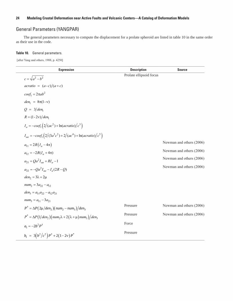
24 Modeling Crustal Deformation near Active Faults and Volcanic Centers—A Catalog of Deformation Models
Table 10. General parameters.
[after Yang and others, 1988, p. 4250]
Expression Description Source
c a b= −2 2Prolate ellipsoid focus
acratio a c a c = +( - ) ( )
coef ab122= π
den1 8 1 = π ν( - )
Q den = 3 1
R den= ( - )1 2 1ν
I coef ac acratio ca = − +( )12 32 ( ) ln( )
I coef a c ac acratio caa = − + +( )13 2 4 52 3 2( ) ( ) ln( )
a R Ia11 2 4= −( )π Newman and others (2006)
a R Ia12 2 4= − +( )π Newman and others (2006)
a Qa I RIaa a212 1= + −
Newman and others (2006)
a Qa I I R Qaa a222 2= − − −( )
Newman and others (2006)
den2 3 2= +λ µ
num a a2 22 123= −
den a a a a3 11 22 12 21= −
num a a3 11 213= −
( )( )†2 2 3 32P P den num num den= ∆ µ −
Pressure Newman and others (2006)
P P den num num den* = ( ) + +( )( )∆ 1 22 2 3 3λ λ µPressure Newman and others (2006)
2 †1 2a b P= −
Force
( ) ( )2 2 † *1 3 2 1 2 b b c P P= + − ν
Pressure
General Parameters (YANGPAR)The general parameters necessary to compute the displacement for a prolate spheroid are listed in table 10 in the same order
as their use in the code.
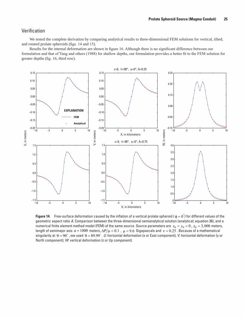
Prolate Spheroid Source (Magma Conduit) 25
men12-7629_fig14
−10 −5 0 5 10−0.20
−0.15
−0.10
−0.05
0.00
0.05
0.10
0.15
−0.20
−0.15
−0.10
−0.05
0.00
0.05
0.10
0.15
U, in
met
ers −10 −5 0 5 10
z=0, θ=90°, φ=0°, A=0.25
X, in kilometers
V, in
met
ers −10 −5 0 5 10
-0.10
-0.05
0.00
0.15
0.20
0.25
W, i
n m
eter
s
−10 −5 0 5 10−1.5
−1.0
−0.5
0.0
0.5
1.0
1.5
−10 −5 0 5 10−1.5
−1.0
−0.5
0.0
0.5
1.0
1.5z=0, θ=90°, φ=0°, A=0.75
X, in kilometers
FEM
Analytical
−10 −5 0 5 100
0.5
1.0
1.5
2.0
2.5
3.0
3.5
4.0
EXPLANATION
Figure 14. Free-surface deformation caused by the inflation of a vertical prolate spheroid ( φ = °0 ) for different values of the geometric aspect ratio A. Comparison between the three-dimensional semianalytical solution (analytical; equation 36), and a numerical finite element method model (FEM) of the same source. Source parameters are x y0 0 0= = , z0 3 000= , meters, length of semimajor axis a = 1000 meters, ∆P µ = 0 1. , µ = 9 6. Gigapascals and ν = 0 25. . Because of a mathematical singularity at θ = 90 , we used θ = 89 99. . U: horizontal deformation (x or East component); V: horizontal deformation (y or North component); W: vertical deformation (z or Up component).
VerificationWe tested the complete derivation by comparing analytical results to three-dimensional FEM solutions for vertical, tilted,
and rotated prolate spheroids (figs. 14 and 15).Results for the internal deformation are shown in figure 16. Although there is no significant difference between our
formulation and that of Yang and others (1988) for shallow depths, our formulation provides a better fit to the FEM solution for greater depths (fig. 16, third row).
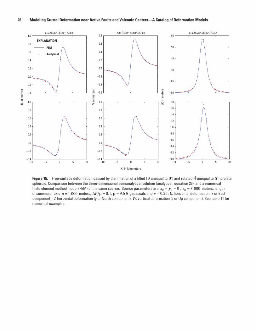
26 Modeling Crustal Deformation near Active Faults and Volcanic Centers—A Catalog of Deformation Models
men12-7629_fig15
−0.4
−0.2
0.0
0.2
0.4
0.6
0.8
1.0
−0.4
−0.2
0.0
0.2
0.4
0.6
0.8
1.0
−0.4
−0.2
0.0
0.2
0.4
0.6
0.8
-0.6
−0.4
−0.2
0.0
0.2
0.4
0.6
0.8
1.0
0.0
0.5
1.0
1.5
2.0
2.5
−10 −5 0 5 10
U, in
met
ers
−10 −5 0 5 10
X, in kilometers
V, in
met
ers
FEM
Analytical
−10 −5 0 5 100.0
0.2
0.4
0.6
0.8
1.0
1.2
1.4
1.6
1.8
W, i
n m
eter
s
z=0, θ=30°, φ=60°, A=0.5 z=0, θ=30°, φ=60°, A=0.5 z=0, θ=30°, φ=60°, A=0.5
EXPLANATION
Figure 15. Free-surface deformation caused by the inflation of a tilted ( θ unequal to 0) and rotated (φunequal to 0) prolate spheroid. Comparison between the three-dimensional semianalytical solution (analytical; equation 36), and a numerical finite element method model (FEM) of the same source. Source parameters are x y0 0 0= = , z0 3 000= , meters, length of semimajor axis a = 1 000, meters, ∆P µ = 0 1. , µ = 9 6. Gigapascals and ν = 0 25. . U: horizontal deformation (x or East component); V: horizontal deformation (y or North component); W: vertical deformation (z or Up component). See table 11 for numerical examples.
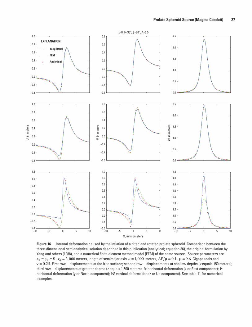
Prolate Spheroid Source (Magma Conduit) 27
men12-7629_fig16
Yang (1988)
FEM
Analytical
U, in
met
ers
V, in
met
ers
W, i
n m
eter
s
−10 −5 0 5 10 −10 −5 0 5 10
X, in kilometers
−10 −5 0 5 10
z=0, θ=30°, φ=60°, A=0.5
−0.4
−0.2
0.0
0.2
0.4
0.6
0.8
1.0
−0.4
−0.2
0.0
0.2
0.4
0.6
0.8
1.0
−0.4
−0.2
0.0
0.2
0.4
0.6
0.8
1.0
1.2
−0.4
−0.2
0.0
0.2
0.4
0.6
0.8
-0.6
−0.4
−0.2
0.0
0.2
0.4
0.6
0.8
-0.6
−0.4
−0.2
1.2
−0.6
0.0
0.2
0.4
0.6
0.8
1.0
0.0
0.5
1.0
1.5
2.0
2.5
0.0
0.5
1.0
1.5
2.0
2.5
0.0
0.5
1.5
2.5
3.5
1.0
2.0
3.0
4.0
4.5
EXPLANATION
Figure 16. Internal deformation caused by the inflation of a tilted and rotated prolate spheroid. Comparison between the three-dimensional semianalytical solution described in this publication (analytical; equation 36), the original formulation by Yang and others (1988), and a numerical finite element method model (FEM) of the same source. Source parameters are x y0 0 0= = , z0 3 000= , meters, length of semimajor axis a = 1 000, meters, ∆P µ = 0 1. , µ = 9 6. Gigapascals and ν = 0 25. . First row—displacements at the free surface; second row—displacements at shallow depths (z equals 150 meters); third row—displacements at greater depths (z equals 1,500 meters). U: horizontal deformation (x or East component); V: horizontal deformation (y or North component); W: vertical deformation (z or Up component). See table 11 for numerical examples.
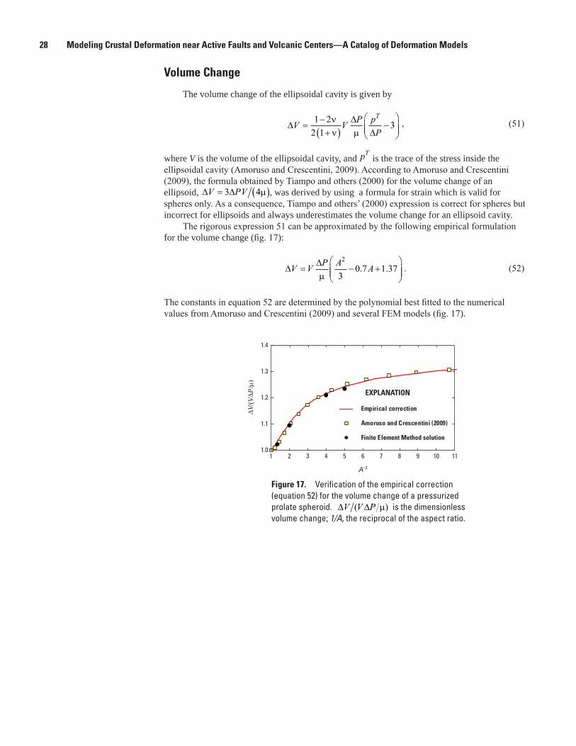
28 Modeling Crustal Deformation near Active Faults and Volcanic Centers—A Catalog of Deformation Models
Volume Change
The volume change of the ellipsoidal cavity is given by
∆∆
∆V V P p
P
T=
−+( )
−
1 22 1
3νν µ
, (51)
where V is the volume of the ellipsoidal cavity, and pT
is the trace of the stress inside the ellipsoidal cavity (Amoruso and Crescentini, 2009). According to Amoruso and Crescentini (2009), the formula obtained by Tiampo and others (2000) for the volume change of an ellipsoid, ∆ ∆V PV= ( )3 4µ , was derived by using a formula for strain which is valid for spheres only. As a consequence, Tiampo and others’ (2000) expression is correct for spheres but incorrect for ellipsoids and always underestimates the volume change for an ellipsoid cavity.
The rigorous expression 51 can be approximated by the following empirical formulation for the volume change (fig. 17):
∆∆V V P A A= − +
µ
2
30 7 1 37. . . (52)
The constants in equation 52 are determined by the polynomial best fitted to the numerical values from Amoruso and Crescentini (2009) and several FEM models (fig. 17).
Figure 17. Verification of the empirical correction (equation 52) for the volume change of a pressurized prolate spheroid. ∆ ∆V V P( )µ is the dimensionless volume change; 1/A, the reciprocal of the aspect ratio.
men12-7629_fig17
1.0
1.1
1.2
1.3
1.4
1 2 3 4 5 6 7 8 9 10 11
A-1
Empirical correction
Amoruso and Crescentini (2009)
Finite Element Method solution
∆V/(V
∆P/µ)
EXPLANATION
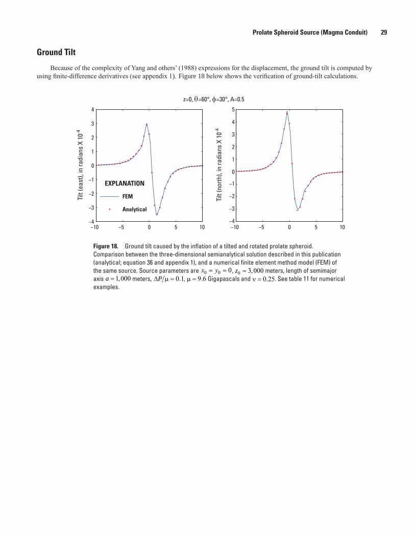
Prolate Spheroid Source (Magma Conduit) 29
Ground Tilt
Because of the complexity of Yang and others’ (1988) expressions for the displacement, the ground tilt is computed by using finite-difference derivatives (see appendix 1). Figure 18 below shows the verification of ground-tilt calculations.
men12-7629_fig18
−10 −5 0 5 10−4
−3
−2
−1
0
1
2
3
4
X, in kilometers
Tilt
(eas
t), in
radi
ans
X 10
-4
−10 −5 0 5 10−4
−3
−2
−1
0
1
2
3
4
5
FEM
Analytical
Tilt
(nor
th),
in ra
dian
s X
10-4
z=0, θ=60°, φ=30°, A=0.5
EXPLANATION
Figure 18. Ground tilt caused by the inflation of a tilted and rotated prolate spheroid. Comparison between the three-dimensional semianalytical solution described in this publication (analytical; equation 36 and appendix 1), and a numerical finite element method model (FEM) of the same source. Source parameters are x y0 0 0= = , z0 3 000= , meters, length of semimajor axis a = 1 000, meters, ∆P µ = 0 1. , µ = 9 6. Gigapascals and ν = 0 25. . See table 11 for numerical examples.
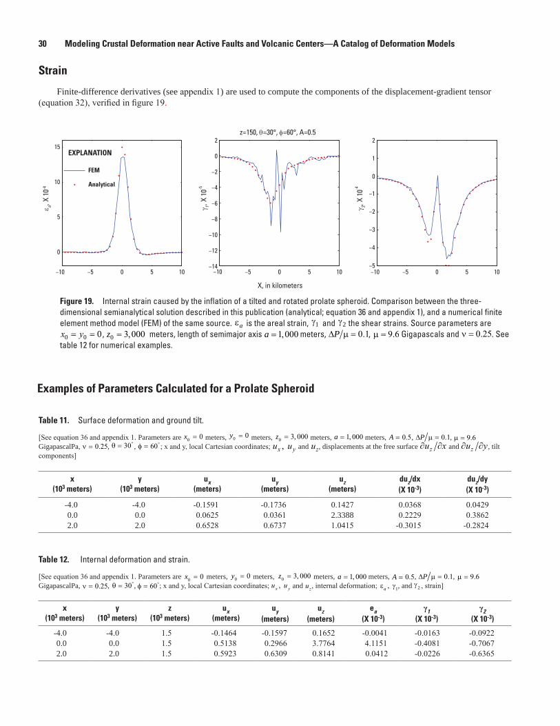
30 Modeling Crustal Deformation near Active Faults and Volcanic Centers—A Catalog of Deformation Models
Strain
Finite-difference derivatives (see appendix 1) are used to compute the components of the displacement-gradient tensor (equation 32), verified in figure 19.
Figure 19. Internal strain caused by the inflation of a tilted and rotated prolate spheroid. Comparison between the three-dimensional semianalytical solution described in this publication (analytical; equation 36 and appendix 1), and a numerical finite element method model (FEM) of the same source. εa
is the areal strain, γ1 and γ2 the shear strains. Source parameters are x y0 0 0= = , z0 3 000= , meters, length of semimajor axis a = 1 000, meters, ∆P µ = 0 1. , µ = 9 6. Gigapascals and ν = 0 25. . See table 12 for numerical examples.
men12-7629_fig19
−10 −5 0 5 10
0
5
10
15
−10 −5 0 5 10−14
−12
−10
−8
−6
−4
−2
0
2
X, in kilometers
FEM
Analytical
−10 −5 0 5 10−5
−4
−3
−2
−1
0
1
2z=150, θ=30°, φ=60°, A=0.5
EXPLANATION
ε a, X
10-4
γ 1, X
10-5
γ 2, X
10-4
Examples of Parameters Calculated for a Prolate Spheroid
Table 11. Surface deformation and ground tilt.
[See equation 36 and appendix 1. Parameters are x0 0= meters, y0 0= meters, z0 3 000= , meters, a = 1 000, meters, A = 0 5. , ∆P µ = 0 1. , µ = 9 6. GigapascalPa, ν = 0 25. , θ = 30 , φ = 60 ; x and y, local Cartesian coordinates; u ux y, and uz, displacements at the free surface ∂ ∂u xz and ∂ ∂u yz , tilt components]
x (103 meters)
y(103 meters)
ux(meters)
uy(meters)
uz(meters)
duz/dx(X 10-3)
duz/dy(X 10-3)
-4.0 -4.0 -0.1591 -0.1736 0.1427 0.0368 0.04290.0 0.0 0.0625 0.0361 2.3388 0.2229 0.38622.0 2.0 0.6528 0.6737 1.0415 -0.3015 -0.2824
Table 12. Internal deformation and strain.
[See equation 36 and appendix 1. Parameters are x0 0= meters, y0 0= meters, z0 3 000= , meters, a = 1 000, meters, A = 0 5. , ∆P µ = 0 1. , µ = 9 6. GigapascalPa, ν = 0 25. , θ = 30, φ = 60; x and y, local Cartesian coordinates; u ux y, and uz, internal deformation; ε γa , 1, and γ2 , strain]
x (103 meters)
y(103 meters)
z(103 meters)
ux(meters)
uy(meters)
uz(meters)
ea(X 10-3)
γ1(X 10-3)
γ2(X 10-3)
-4.0 -4.0 1.5 -0.1464 -0.1597 0.1652 -0.0041 -0.0163 -0.09220.0 0.0 1.5 0.5138 0.2966 3.7764 4.1151 -0.4081 -0.70672.0 2.0 1.5 0.5923 0.6309 0.8141 0.0412 -0.0226 -0.6365
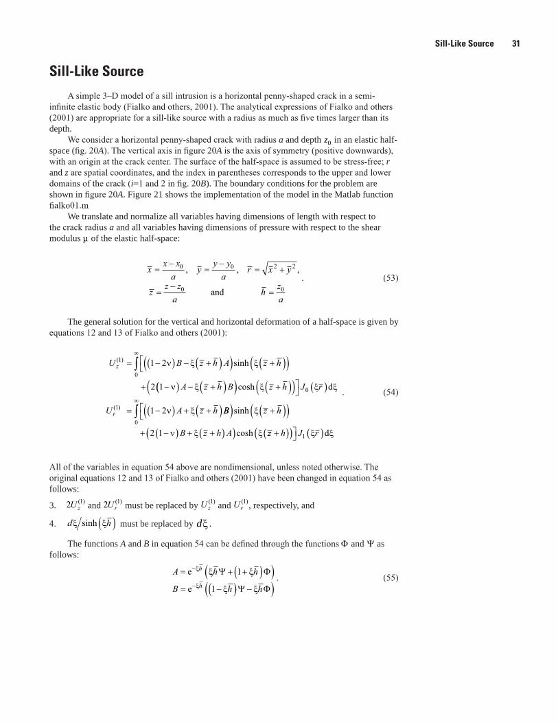
Sill-Like Source 31
A simple 3–D model of a sill intrusion is a horizontal penny-shaped crack in a semi-infinite elastic body (Fialko and others, 2001). The analytical expressions of Fialko and others (2001) are appropriate for a sill-like source with a radius as much as five times larger than its depth.
We consider a horizontal penny-shaped crack with radius a and depth z0 in an elastic half-space (fig. 20A). The vertical axis in figure 20A is the axis of symmetry (positive downwards), with an origin at the crack center. The surface of the half-space is assumed to be stress-free; r and z are spatial coordinates, and the index in parentheses corresponds to the upper and lower domains of the crack (i=1 and 2 in fig. 20B). The boundary conditions for the problem are shown in figure 20A. Figure 21 shows the implementation of the model in the Matlab function fialko01.m
We translate and normalize all variables having dimensions of length with respect to the crack radius a and all variables having dimensions of pressure with respect to the shear modulus µ of the elastic half-space:
x
x xa
yy ya
r x y
zz za
hza
=−
=−
= +
=−
=
0 0 2 2
0 0
, , ,
and. (53)
The general solution for the vertical and horizontal deformation of a half-space is given by equations 12 and 13 of Fialko and others (2001):
U B z h A z hz( ) sinh1
0
1 2
2 1
= −( ) − +( )( ) +( )( )
+ −
∞
∫ ν ξ ξ
ν (( ) − +( )( ) +( )( ) ( )
= −( ) + +( )
A z h B z h J r
U A z hr
ξ ξ ξ ξ
ν ξ
cosh
( )
0
1 1 2
d
BB z h
B z h A
( ) +( )( )
+ −( ) + +( )( )
∞
∫ sinh
cosh
ξ
ν ξ ξ0
2 1 zz h J r+( )( ) ( )1 ξ ξd
. (54)
All of the variables in equation 54 above are nondimensional, unless noted otherwise. The original equations 12 and 13 of Fialko and others (2001) have been changed in equation 54 as follows:
3. 2 1Uz( ) and 2 1Ur
( ) must be replaced by Uz( )1 and Ur
( )1 , respectively, and
4. d hξ ξsinh ( ) must be replaced by dx .
The functions A and B in equation 54 can be defined through the functions Φ and Ψ as follows:
A h h
B h h
h
h
= + +( )( )= −( ) −( )
−
−
e
e
ξ
ξ
ξ ξ
ξ ξ
Ψ Φ
Ψ Φ
1
1. (55)
Sill-Like Source
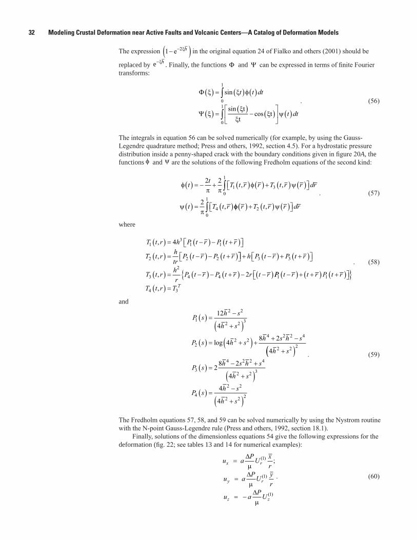
32 Modeling Crustal Deformation near Active Faults and Volcanic Centers—A Catalog of Deformation Models
The expression 1 e−( )−2ξh in the original equation 24 of Fialko and others (2001) should be
replaced by e−ξh . Finally, the functions Φ and Ψ can be expressed in terms of finite Fourier transforms:
Φ
Ψ
ξ ξ φ
ξξ
ξξ ψ
( ) = ( ) ( )
( ) = ( )− ( )
( )
∫
∫
sin t t dt
t dt
0
1
0
1 sin tt
cos t
. (56)
The integrals in equation 56 can be solved numerically (for example, by using the Gauss-Legendre quadrature method; Press and others, 1992, section 4.5). For a hydrostatic pressure distribution inside a penny-shaped crack with the boundary conditions given in figure 20A, the functions φ and y are the solutions of the following Fredholm equations of the second kind:
φ
π πφ ψ
ψπ
t t T t r r T t r r dr
t T t r
( ) = − + ( ) ( ) + ( ) ( )
( ) = ( )
∫2 2
2
1 30
1
4
, ,
, φφ ψr T t r r dr( ) + ( ) ( ) ∫ 20
1
,
. (57)
where
T t r h
t r
P t r P t r
T htrP t r P t r
13
1 1
2 2 2
4,
,
( ) = −
( )
−( ) +( )
= −( ) − +( ) + −( ) + +( )
−( ) +( )( ) = − − −( )
h P t r P t r
t r t rT t r hrP P r t r
3 3
3
2
4 4 2, PP t r t r P t r
t rT T T1 1
4 3
−( ) + +( ) +( ) { }( ) =,
. (58)
and
P s h s
h s
P s h s h s h s
h s
1
2 2
2 2 3
22 2
4 2 2 4
2 2
12
4
4 8 2
4
( ) = −
+( )( ) = +( ) + + −
+log
(( )( ) = − +
+( )( ) = −
+( )
2
3
4 2 2 4
2 2 3
4
2 2
2 2 2
2 8 2
4
4
4
P s h s h s
h s
P s h s
h s
. (59)
The Fredholm equations 57, 58, and 59 can be solved numerically by using the Nystrom routine with the N-point Gauss-Legendre rule (Press and others, 1992, section 18.1).
Finally, solutions of the dimensionless equations 54 give the following expressions for the deformation (fig. 22; see tables 13 and 14 for numerical examples):
u a PU xr
u a PU yr
u a PU
x r
y r
z z
=
=
= −
∆
∆
∆
µ
µ
µ
( )
( )
( )
;1
1
1
. (60)
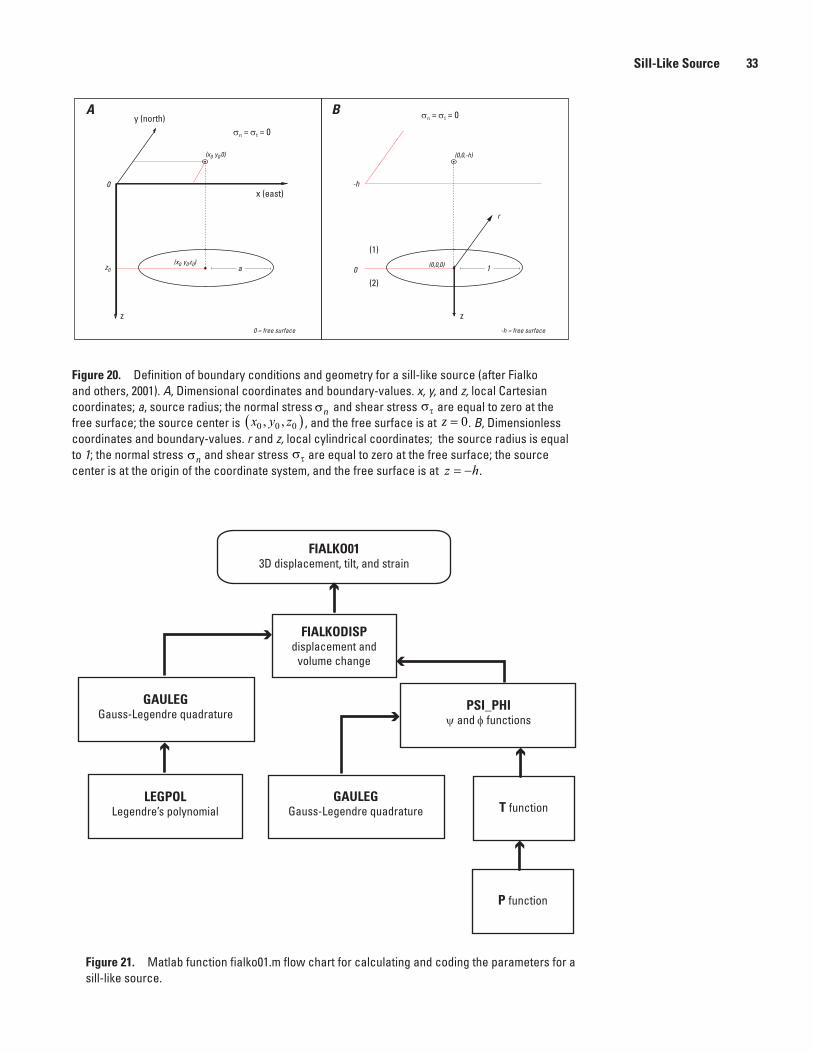
Sill-Like Source 33
Figure 20. Definition of boundary conditions and geometry for a sill-like source (after Fialko and others, 2001). A, Dimensional coordinates and boundary-values. x, y, and z, local Cartesian coordinates; a, source radius; the normal stress σn and shear stress στ are equal to zero at the free surface; the source center is x y z0 0 0, ,( ) , and the free surface is at z = 0. B, Dimensionless coordinates and boundary-values. r and z, local cylindrical coordinates; the source radius is equal to 1; the normal stress σn and shear stress στ are equal to zero at the free surface; the source center is at the origin of the coordinate system, and the free surface is at z h= − .
men12-7629_fig20
x (east)
y (north)
z
(x0 y0 0)
σn = σt = 0
z0
BA
(1)
(2)
a
z
(0,0,0)
σn = σt = 0
0 1
0 -h
r
0 = free surface -h = free surface
(0,0,-h)¤ ¤
(x0 y0 z0)
men12-7629_fig21
FIALKO013D displacement, tilt, and strain
FIALKODISPdisplacement and
volume change
GAULEGGauss-Legendre quadrature
PSI_PHIψ and φ functions
LEGPOLLegendre’s polynomial
GAULEGGauss-Legendre quadrature T function
P function
Figure 21. Matlab function fialko01.m flow chart for calculating and coding the parameters for a sill-like source.
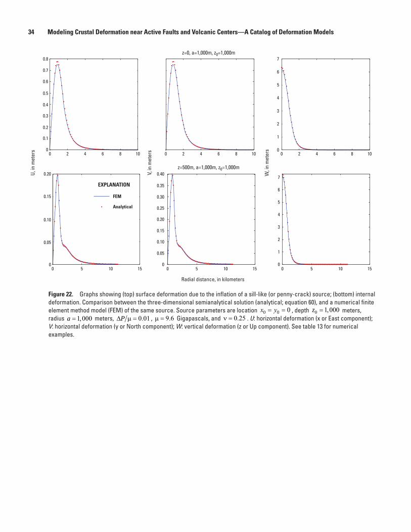
34 Modeling Crustal Deformation near Active Faults and Volcanic Centers—A Catalog of Deformation Models
Figure 22. Graphs showing (top) surface deformation due to the inflation of a sill-like (or penny-crack) source; (bottom) internal deformation. Comparison between the three-dimensional semianalytical solution (analytical; equation 60), and a numerical finite element method model (FEM) of the same source. Source parameters are location x y0 0 0= = , depth z0 1 000= , meters, radius a = 1 000, meters, ∆P µ = 0 01. , µ = 9 6. Gigapascals, and ν = 0 25. . U: horizontal deformation (x or East component); V: horizontal deformation (y or North component); W: vertical deformation (z or Up component). See table 13 for numerical examples.
men12-7629_fig22
0.2
0.3
0.4
0.5
0.6
0.7
0.8
0.1
0
0.05
0.10
0.15
0.20
0 0
0.05
0.40
0.10
0.15
0.20
0.25
0.30
0.35
0 2 4 6 8 10
U, in
met
ers
0 2 4 6 8 10
z=0, a=1,000m, z0=1,000m
Radial distance, in kilometers
V, in
met
ers 0 2 4 6 8 10
0
1
2
3
4
5
6
7
W, i
n m
eter
s0 5 10 15 0 5 10 15
z=500m, a=1,000m, z0=1,000m
0 5 10 150
1
2
3
4
5
6
7
FEM
Analytical
EXPLANATION
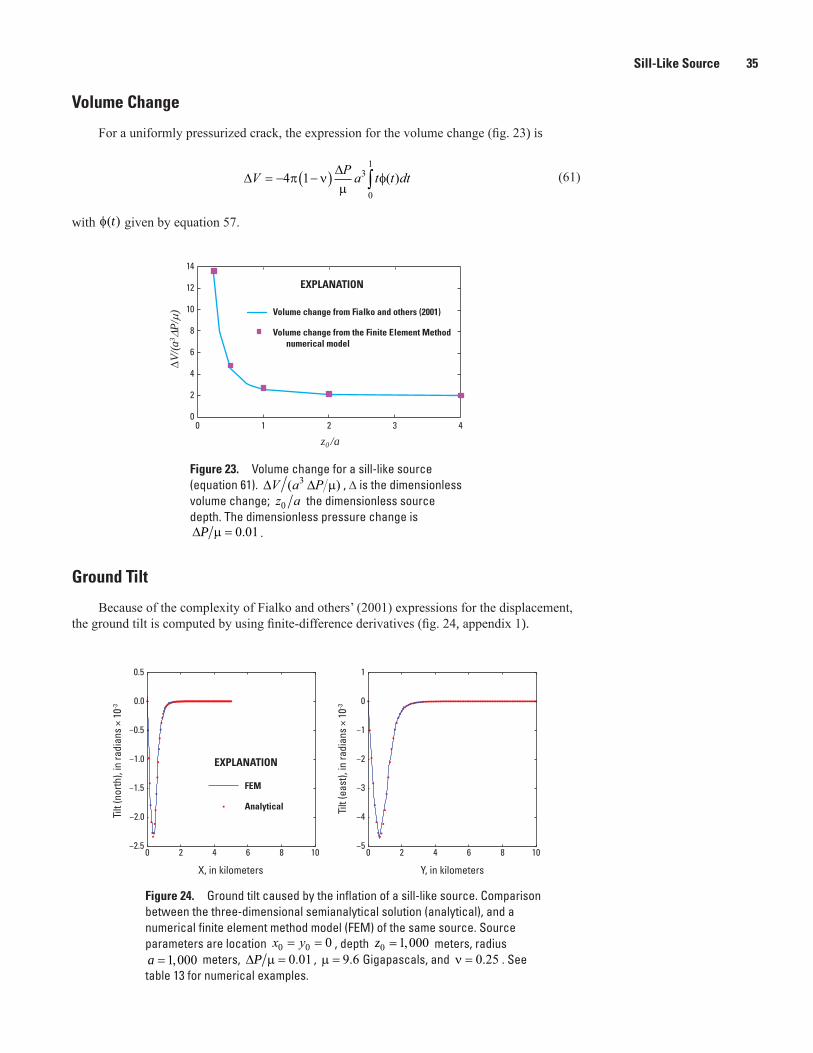
Sill-Like Source 35
Volume Change
For a uniformly pressurized crack, the expression for the volume change (fig. 23) is
∆∆V P a t t dt= − −( ) ∫4 1 3
0
1
π νµ
φ( ) (61)
with φ( )t given by equation 57.
Ground Tilt
Because of the complexity of Fialko and others’ (2001) expressions for the displacement, the ground tilt is computed by using finite-difference derivatives (fig. 24, appendix 1).
Figure 23. Volume change for a sill-like source (equation 61). ∆ ∆V a P( )3 µ , ∆ is the dimensionless volume change; z a0 the dimensionless source depth. The dimensionless pressure change is ∆P µ = 0 01. .
men12-7629_fig24
0 2 4 6 8 10−2.5
−2.0
−1.5
−1.0
−0.5
0.0
0.5
X, in kilometers
Tilt
(nor
th),
in ra
dian
s ×
10-3
0 2 4 6 8 10−5
−4
−3
−2
−1
0
1
Y, in kilometers
Tilt
(eas
t), in
radi
ans
× 10
-3
FEM
Analytical
EXPLANATION
Figure 24. Ground tilt caused by the inflation of a sill-like source. Comparison between the three-dimensional semianalytical solution (analytical), and a numerical finite element method model (FEM) of the same source. Source parameters are location x y0 0 0= = , depth z0 1 000= , meters, radius a = 1 000, meters, ∆P µ = 0 01. , µ = 9 6. Gigapascals, and ν = 0 25. . See table 13 for numerical examples.
men12-7629_fig23
0
2
4
6
8
10
12
14
0 1 2 3 4
Volume change from Fialko and others (2001)
Volume change from the Finite Element Method numerical model
EXPLANATION
∆V/(a
3 ∆P/µ)
z0 /a
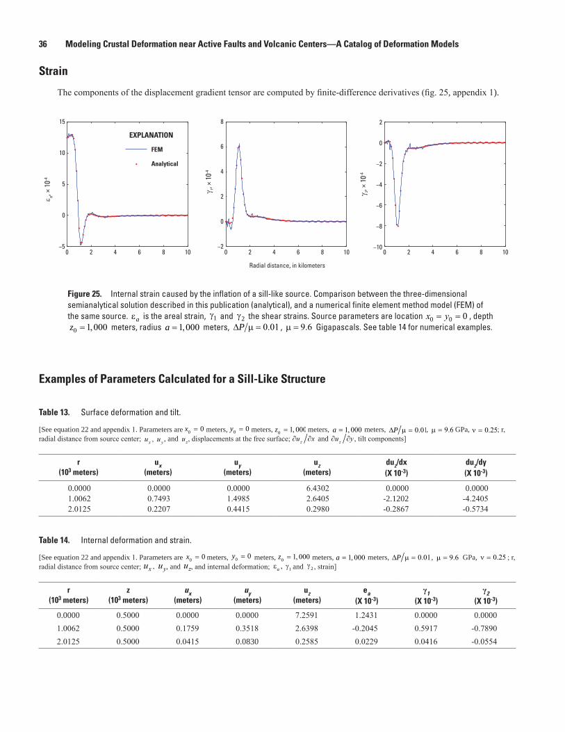
36 Modeling Crustal Deformation near Active Faults and Volcanic Centers—A Catalog of Deformation Models
Strain
The components of the displacement gradient tensor are computed by finite-difference derivatives (fig. 25, appendix 1).
men12-7629_fig25
0 2 4 6 8 10−5
0
5
10
15
ε a, × 1
0-4
0 2 4 6 8 10−2
0
2
4
6
8
Radial distance, in kilometers
γ 1, ×
10-4
0 2 4 6 8 10−10
−8
−6
−4
−2
0
2
γ 2, ×
10-4
FEM
Analytical
EXPLANATION
Figure 25. Internal strain caused by the inflation of a sill-like source. Comparison between the three-dimensional semianalytical solution described in this publication (analytical), and a numerical finite element method model (FEM) of the same source. εa
is the areal strain, γ1 and γ2 the shear strains. Source parameters are location x y0 0 0= = , depth z0 1 000= , meters, radius a = 1 000, meters, ∆P µ = 0 01. , µ = 9 6. Gigapascals. See table 14 for numerical examples.
Examples of Parameters Calculated for a Sill-Like Structure
Table 13. Surface deformation and tilt.
[See equation 22 and appendix 1. Parameters are x0 0= meters, y0 0= meters, z0 1 000= , meters, a = 1 000, meters, ∆P µ = 0 01. , µ = 9 6. GPa, ν = 0 25. ; r, radial distance from source center; u ux y, , and uz, displacements at the free surface; ∂ ∂u xz and ∂ ∂u yz , tilt components]
r (103 meters)
ux (meters)
uy (meters)
uz (meters)
duz/dx(X 10-3)
duz/dy(X 10-3)
0.0000 0.0000 0.0000 6.4302 0.0000 0.00001.0062 0.7493 1.4985 2.6405 -2.1202 -4.24052.0125 0.2207 0.4415 0.2980 -0.2867 -0.5734
Table 14. Internal deformation and strain.
[See equation 22 and appendix 1. Parameters are x0 0= meters, y0 0= meters, z0 1 000= , meters, a = 1 000, meters, ∆P µ = 0 01. , µ = 9 6. GPa, ν = 0 25. ; r, radial distance from source center; u ux y, , and uz, and internal deformation; ε γa , 1 and γ2 , strain]
r (103 meters)
z(103 meters)
ux(meters)
uy(meters)
uz(meters)
ea(X 10-3)
γ1(X 10-3)
γ2(X 10-3)
0.0000 0.5000 0.0000 0.0000 7.2591 1.2431 0.0000 0.00001.0062 0.5000 0.1759 0.3518 2.6398 -0.2045 0.5917 -0.78902.0125 0.5000 0.0415 0.0830 0.2585 0.0229 0.0416 -0.0554
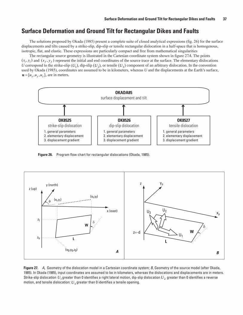
Surface Deformation and Ground Tilt for Rectangular Dikes and Faults 37
Surface Deformation and Ground Tilt for Rectangular Dikes and FaultsThe solutions proposed by Okada (1985) present a complete suite of closed analytical expressions (fig. 26) for the surface
displacements and tilts caused by a strike-slip, dip-slip or tensile rectangular dislocation in a half-space that is homogenous, isotropic, flat, and elastic. These expressions are particularly compact and free from mathematical singularities
The rectangular source geometry is illustrated in the Cartesian coordinate system shown in figure 27A. The points ( , )x yi i and ( , )x yf f represent the initial and end coordinates of the source trace at the surface. The elementary dislocations U correspond to the strike-slip (U1), dip-slip (U2), or tensile (U3) component of an arbitrary dislocation. In the convention used by Okada (1985), coordinates are assumed to be in kilometers, whereas U and the displacements at the Earth’s surface, u = [ , , ]u u ux y z , are in meters.
Figure 26. Program flow chart for rectangular dislocations (Okada, 1985).
Figure 27. A, Geometry of the dislocation model in a Cartesian coordinate system; B, Geometry of the source model (after Okada, 1985). In Okada (1985), input coordinates are assumed to be in kilometers, whereas the dislocations and displacements are in meters. Strike-slip dislocation U1 greater than 0 identifies a right lateral motion, dip-slip dislocation U2 greater than 0 identifies a reverse motion, and tensile dislocation: U3 greater than 0 identifies a tensile opening.
men12-7629_fig26
OKADA85surface displacement and tilt
OK8525strike-slip dislocation
1. general parameters2. elementary displacement3. displacement gradient
OK8526dip-slip dislocation
1. general parameters2. elementary displacement3. displacement gradient
OK8527tensile dislocation
1. general parameters2. elementary displacement3. displacement gradient
men12-7629_fig27
z (up)y (north)
x (east)
(xi,yi)
δ
(xf,yf)φ
zt
zb L
W
A B
δ
ypz
xp
z=-d
U3
L
WU1
U2
(x0,y0,z0)
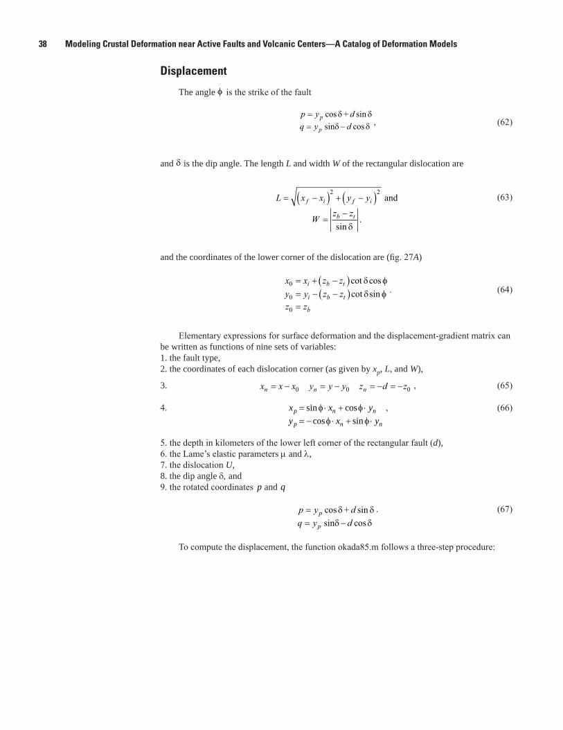
38 Modeling Crustal Deformation near Active Faults and Volcanic Centers—A Catalog of Deformation Models
Displacement
The angle φ is the strike of the fault
p y dq y d
p
p
== −
cos sincos
δ δδ δ
+ sin , (62)
and δ is the dip angle. The length L and width W of the rectangular dislocation are
L x x y y
Wz z
f i f i
b t
= −( ) + −( )=
−
2 2 and
sin.
δ
(63)
and the coordinates of the lower corner of the dislocation are (fig. 27A)
x x z zy y z zz z
i b t
i b t
b
0
0
0
= + −( )= − −( )=
cot coscot sin
δ φδ φ . (64)
Elementary expressions for surface deformation and the displacement-gradient matrix can be written as functions of nine sets of variables: 1. the fault type, 2. the coordinates of each dislocation corner (as given by xp, L, and W),
3. x x x y y y z d zn n n= − = − = − = −0 0 0 , (65)
4. sin cos cos sin
p n n
p n n
x x yy x y
= φ⋅ + φ⋅= − φ⋅ + φ⋅
, (66)
5. the depth in kilometers of the lower left corner of the rectangular fault (d), 6. the Lame’s elastic parameters µ and λ,7. the dislocation U, 8. the dip angle δ, and 9. the rotated coordinates p and q
p y dq y d
p
p
== −
cos sincos
δ δδ δ
+ sin
. (67)
To compute the displacement, the function okada85.m follows a three-step procedure:
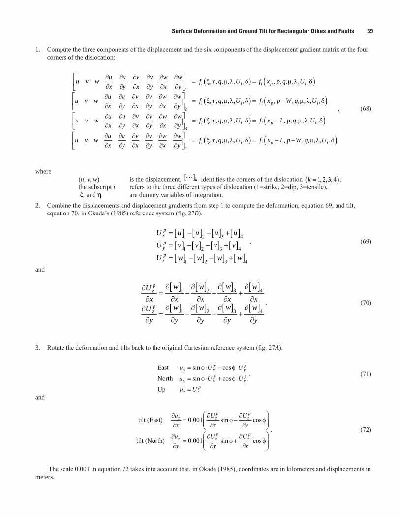
Surface Deformation and Ground Tilt for Rectangular Dikes and Faults 39
1. Compute the three components of the displacement and the six components of the displacement gradient matrix at the four corners of the dislocation:
( ) ( )
( ) ( )1
2
3
, , , , , , , , , , , ,
, , , , , , , , , , , ,
, , ,
i i i p i
i i i p i
i
u u v v w wu v w f q U f x p q Ux y x y x yu u v v w wu v w f q U f x p W q Ux y x y x yu u v v w wu v w f qx y x y x y
∂ ∂ ∂ ∂ ∂ ∂= x η µ λ δ = µ λ δ ∂ ∂ ∂ ∂ ∂ ∂
∂ ∂ ∂ ∂ ∂ ∂= x η µ λ δ = − µ λ δ ∂ ∂ ∂ ∂ ∂ ∂
∂ ∂ ∂ ∂ ∂ ∂= x η µ ∂ ∂ ∂ ∂ ∂ ∂
( ) ( )
( ) ( )4
, , , , , , , , ,
, , , , , , , , , , , ,
i i p i
i i i p i
U f x L p q U
u u v v w wu v w f q U f x L p W q Ux y x y x y
λ δ = − µ λ δ
∂ ∂ ∂ ∂ ∂ ∂= x η µ λ δ = − − µ λ δ ∂ ∂ ∂ ∂ ∂ ∂
, (68)
where (u, v, w) is the displacement, [ ] k identifies the corners of the dislocation k =( )1 2 3 4, , , , the subscript i refers to the three different types of dislocation (1=strike, 2=dip, 3=tensile), x and η are dummy variables of integration.2. Combine the displacements and displacement gradients from step 1 to compute the deformation, equation 69, and tilt,
equation 70, in Okada’s (1985) reference system (fig. 27B).
[ ] [ ] [ ] [ ][ ] [ ] [ ] [ ][ ] [ ] [ ] [ ]
1 2 3 4
1 2 3 4
1 2 3 4
pxpypz
U u u u u
U v v v v
U w w w w
= − − +
= − − +
= − − +
, (69)
and
[ ] [ ] [ ] [ ]
[ ] [ ] [ ] [ ]
31 2 4
31 2 4
pz
pz
ww w wUx x x x x
ww w wUy y y y y
∂∂ ∂ ∂∂= − − +
∂ ∂ ∂ ∂ ∂∂∂ ∂ ∂∂
= − − +∂ ∂ ∂ ∂ ∂
. (70)
3. Rotate the deformation and tilts back to the original Cartesian reference system (fig. 27A):
East
North
Up
u U Uu U Uu U
x xp
yp
y yp
xp
z zp
= ⋅ − ⋅
= ⋅ + ⋅
=
sin cos
sin cos
φ φ
φ φ, (71)
and
tilt (East)
tilt (N
∂∂
=∂∂
−∂∂
ux
Ux
Uy
z zp
zp
0 001. sin cosφ φ
oorth)∂∂
=∂∂
+∂∂
uy
Uy
Ux
z zp
zp
0 001. sin cosφ φ
. (72)
The scale 0.001 in equation 72 takes into account that, in Okada (1985), coordinates are in kilometers and displacements in meters.
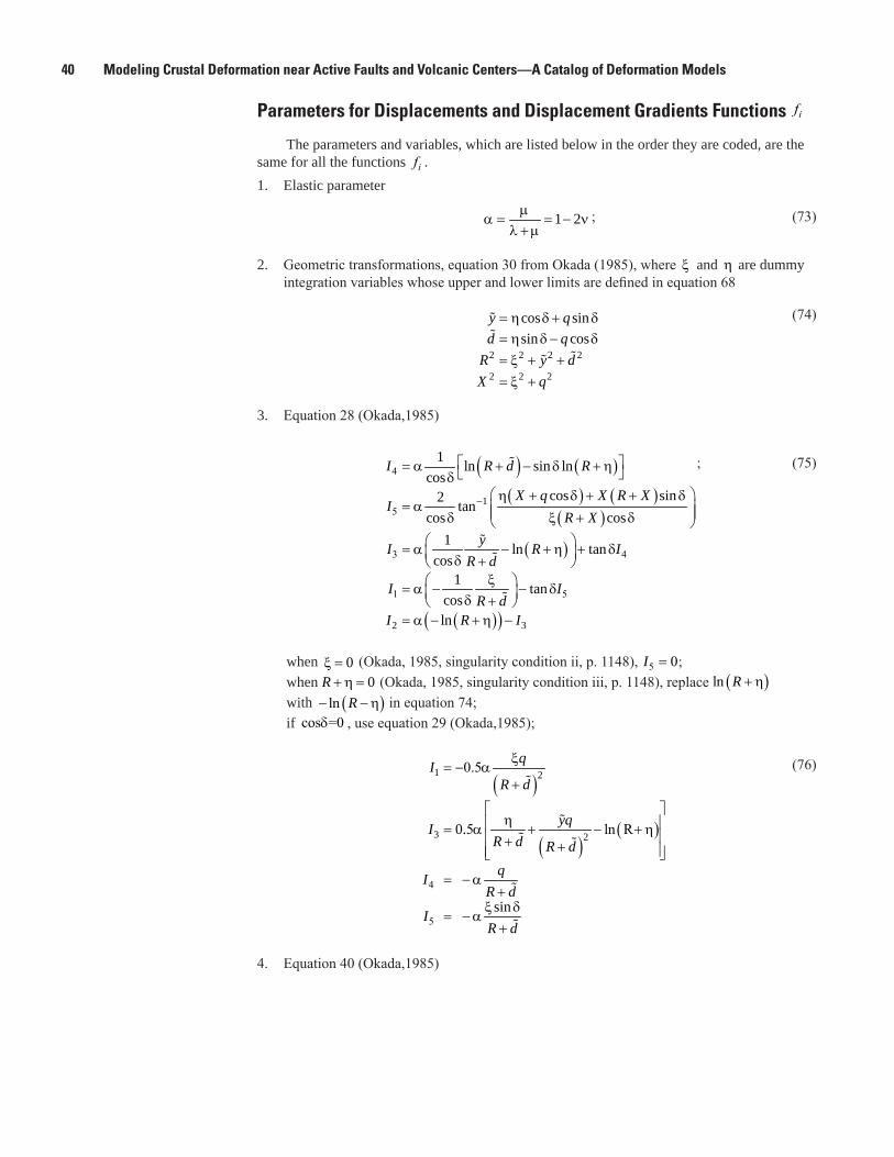
40 Modeling Crustal Deformation near Active Faults and Volcanic Centers—A Catalog of Deformation Models
Parameters for Displacements and Displacement Gradients Functions fi
The parameters and variables, which are listed below in the order they are coded, are the same for all the functions fi . 1. Elastic parameter
1 2µα = = − ν
λ + µ; (73)
2. Geometric transformations, equation 30 from Okada (1985), where x and η are dummy integration variables whose upper and lower limits are defined in equation 68
2 2 2 2
2 2 2
cos sinsin cos
y qd q
R y dX q
= η δ + δ= η δ − δ= x + += x +
(74)
3. Equation 28 (Okada,1985)
( ) ( )
( ) ( )( )
( )
( )( )
4
15
3 4
1 5
2 3
1 ln sin lncos
cos sin2 tancos cos
1 ln tancos
1 tancosln
I R d R
X q X R XI
R XyI R I
R d
I IR d
I R I
−
= α + − δ + η δ η + δ + + δ
= α δ x + δ = α − + η + δ δ +
x = α − − δ δ + = α − + η −
; (75)
when ξ = 0 (Okada, 1985, singularity condition ii, p. 1148), I5 0= ;when R + =η 0 (Okada, 1985, singularity condition iii, p. 1148), replace ln R +( )ηwith − −( )ln R η in equation 74;if cos =0δ , use equation 29 (Okada,1985);
( )
( )( )
5
1
2
4
2
3
0.5
0.
5 ln R
sin
qIR d
yqIR d R dq
R d
RI
d
I
x= − α
+
η = α + − + η + +
α+
x
= −
−δ
α+
=
(76)
4. Equation 40 (Okada,1985)
Surface Deformation and Ground Tilt for Rectangular Dikes and Faults 41
( )
( )
3
1
2 3
1 1cos
1 sin 1cos
sin cos 1
q yKR R R R d
KR RR R d
qK KR R R
= α −
δ + η + x δ = α −
δ + η + δ δ
= α − + − + η
; (77)
if cos 0δ = , use equation 41 from Okada (1985):
( )
( )
1 2
2
3 1
qKR R d
sinKR d R R d
αx=
+
δ x = α − + +
(78)
5. Equation 34 (Okada 1985)
( )
( )
3
3
2
1 2
2 1
2
4
2
1
1 1cos
1 tan
tan
1
cos sin 1
os
c
K
J JR R
qJ JR R
JR dR R d
yJ K
R
R R d
x = α − − δ ++
x= α −
δ +
α
δ
δ
x= − − + η
δ δ= − − − + η
α
; (79)
if cos 0δ = , use equation 35 from Okada,1985)
( ) ( )
( ) ( )
2
1 2
2
2 2
20.5 1
sin 20.5 1
qJR R dR d
qJR R dR d
x = α − ++ x δ = α − ++
(80)
6. Equation 36 (Okada,1985)
( ) ( )2 23 3
2 2c n
R RA AR R R R
+ x + η= =
+ x + η (81)
7. If R + =η 0 (Okada, 1985, singularity condition iii, p. 1148), replace ln R +( )η with
− −( )ln R η and set 1 0R +
=η
.

42 Modeling Crustal Deformation near Active Faults and Volcanic Centers—A Catalog of Deformation Models
Elementary Function f1 for a Strike-Slip Fault
Elementary Displacement (Okada, 1985, equation 25)
u U qR R qR
I
v U yqR R
= −+
+
+
= −+
−1 11
1
21
21
πξ
ηξη
δ
π η
tan sin
+++
+
= −+
++
+
qR
I
w U dqR R
qR
I
cos sin
sin sin
δη
δ
π ηδ
ηδ
1
21 1
2
14
; (82)
if 0q = (Okada, 1985, singularity condition i, p. 1148), then
11
1 sin2U qu I
R R x
= − + δ π + η . (83)
Displacement Gradient (Okada, 1985, equation 37)
1 2
21
13
23 3
cos sin
sincos cos si
2
n2
n
n
w qq A Kx Rw dq yqqA Ky RR
UR
U π
π
∂ x = −x δ + − δ ∂ ∂ δ = δ + x δ − + − δ ∂
(84)
Elementary Function f2 for a Dip-Slip Fault
Elementary Displacement (Okada, 1985, equation 26)
23
121
125
sin cos2
1 cos tan sin cos2
1 sin tan sin cos2
U qu IR
U yqv IR R qR
U dqw IR R qR
−
−
= − − δ δ π xη
= − + δ − δ δ π + x xη
= − + δ − δ δ π + x
; (85)
if 0q = (Okada, 1985, singularity condition i, p. 1148), then
21
25
1 sin cos2
1 sin cos2
U yqv IR R
U dqw IR R
= − − δ δ π + x
= − − δ δ
π + x
(86)
Surface Deformation and Ground Tilt for Rectangular Dikes and Faults 43
Displacement Gradient (Okada, 1985, equation 38)
3
2
32
1
2
2 1 sin sin sin co
sin 1 sin o
s
s
12
c
c
U
U dydqA
w dq q
KR R
Kx R RRwy R R
∂ δ= + + δ δ
∂ + η ∂ δ
π
x= − + δ +
πδ δ
∂ + x + η
(87)
Elementary Function f3 for a Tensile Crack
Elementary Displacement (Okada, 1985, equation 27)
223
3
1 231
1 235
sin2
1 sin tan sin2
1 cos tan sin
1
2
1
1
U qu I
U dq qv I
R R
R
R
R R r qr
U yq qw IR R r qr
−
−
= − δ π
x xη= − − δ − − δ π + x
x xη= + δ − − δ
+ η
+
π + x
η
+ η
; (88)
if 0q = (Okada, 1985, singularity condition i, p. 1148), then
vU dq
R Rqr
I
wU yq
R
R= −
+−
−
=
+3
12
3
21
21
1π ξ
δξ
δ
π
η
sin sin
RRqr
IR+
+
−
+ξ
δξ
δη
cos sin15
2 (89)
Displacement Gradient (Okada, 1985, equation 38)
∂∂
= − − +
∂∂
= −
wx
qR
q A K
wy
y
U
U
n3
3
2
33
32
2
2
πδ
π
δδ
sin cos sin
sin δδ δ ξ δ δξ
δ+ + −+
−
d q A q A q
R RKc ncos sin cos sin2 2
122 1
. (90)
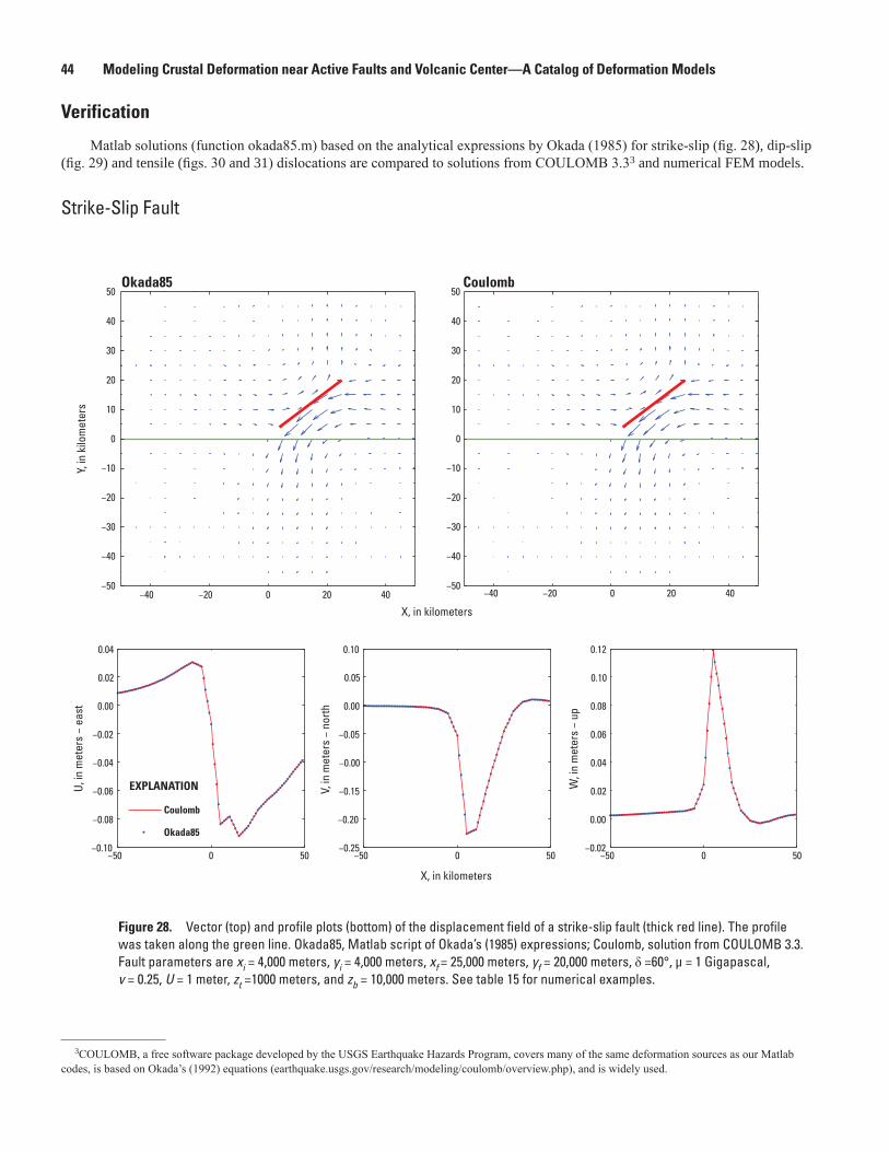
44 Modeling Crustal Deformation near Active Faults and Volcanic Center—A Catalog of Deformation Models
Verification
Matlab solutions (function okada85.m) based on the analytical expressions by Okada (1985) for strike-slip (fig. 28), dip-slip (fig. 29) and tensile (figs. 30 and 31) dislocations are compared to solutions from COULOMB 3.33 and numerical FEM models.
Strike-Slip Fault
Figure 28. Vector (top) and profile plots (bottom) of the displacement field of a strike-slip fault (thick red line). The profile was taken along the green line. Okada85, Matlab script of Okada’s (1985) expressions; Coulomb, solution from COULOMB 3.3. Fault parameters are xi = 4,000 meters, yi = 4,000 meters, xf = 25,000 meters, yf = 20,000 meters, δ =60°, µ = 1 Gigapascal, v = 0.25, U = 1 meter, zt =1000 meters, and zb = 10,000 meters. See table 15 for numerical examples.
men12-7629_fig28
−40 −20 0 20 40
Okada85
X, in kilometers
Y, in
kilo
met
ers
−40 −20 0 20 40−50
−40
−30
−20
−10
0
10
20
30
40
−50
−40
−30
−20
−10
0
10
20
30
40
5050Coulomb
−50 0 50−0.10
−0.08
−0.06
−0.04
−0.02
0.00
0.02
0.04
U, in
met
ers
− ea
st
−50 0 50−0.25
−0.20
−0.15
−0.00
−0.05
0.00
0.05
0.10
V, in
met
ers
− no
rth
Coulomb
Okada85
−50 0 50−0.02
0.00
0.02
0.04
0.06
0.08
0.10
0.12
W, i
n m
eter
s −
up
X, in kilometers
EXPLANATION
3COULOMB, a free software package developed by the USGS Earthquake Hazards Program, covers many of the same deformation sources as our Matlab codes, is based on Okada’s (1992) equations (earthquake.usgs.gov/research/modeling/coulomb/overview.php), and is widely used.
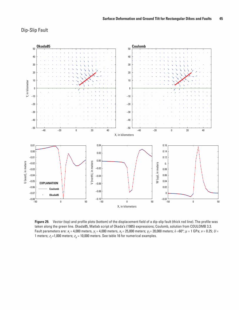
Surface Deformation and Ground Tilt for Rectangular Dikes and Faults 45
Dip-Slip Fault
men12-7629_fig29
EXPLANATION
Okada85
X, in kilometers
Y, in
kilo
met
er
Coulomb
−50 0 50−0.08
−0.07
−0.06
−0.05
−0.04
−0.03
−0.02
−0.01
0.00
0.01
U (e
ast),
in m
eter
s
−50 0 50−0.10
−0.08
−0.06
−0.04
−0.02
0.00
0.02
0.04
V (n
orth
), in
met
ers
X, in kilometers
−50 0 50−0.02
0
0.02
0.04
0.06
0.08
0.
0.12
0.14
0.16
W (u
p), i
n m
eter
s
Coulomb
Okada85
−40 −20 0 20 40 −40 −20 0 20 40−50
−40
−30
−20
−10
0
10
20
30
40
50
−50
−40
−30
−20
−10
0
10
20
30
40
50
Figure 29. Vector (top) and profile plots (bottom) of the displacement field of a dip-slip fault (thick red line). The profile was taken along the green line. Okada85, Matlab script of Okada’s (1985) expressions; Coulomb, solution from COULOMB 3.3. Fault parameters are: xi = 4,000 meters, yi = 4,000 meters, xf = 25,000 meters; yf = 20,000 meters; δ =60°; µ = 1 GPa; v = 0.25; U = 1 meters; zt =1,000 meters; zb = 10,000 meters. See table 16 for numerical examples.
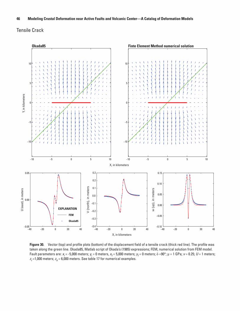
46 Modeling Crustal Deformation near Active Faults and Volcanic Center—A Catalog of Deformation Models
men12-7629_fig30
EXPLANATION
−10 −5 0 5 10
−10
−5
0
5
10
Okada85
X, in kilometers
Y, in
kilo
met
ers
−10 −5 0 5 10
−10
−5
0
5
10
Finte Element Method numerical solution
−40 −20 0 20 40−0.05
0.00
0.05
U (e
ast),
in m
eter
s
−40 −20 0 20 40−0.4
−0.3
−0.2
−0.1
0.0
0.1
0.2
0.3
V (n
orth
), in
met
ers
X, in kilometers
−40 −20 0 20 40−0.10
−0.05
0.00
0.05
0.10
0.15
w (u
p), i
n m
eter
s
FEM
Okada85
Figure 30. Vector (top) and profile plots (bottom) of the displacement field of a tensile crack (thick red line). The profile was taken along the green line. Okada85, Matlab script of Okada’s (1985) expressions; FEM, numerical solution from FEM model. Fault parameters are: xi = -5,000 meters; yi = 0 meters, xf = 5,000 meters; yf = 0 meters; δ =90°; µ = 1 GPa; v = 0.25; U = 1 meters; zt =1,000 meters; zb = 6,000 meters. See table 17 for numerical examples.
Tensile Crack

Surface Deformation and Ground Tilt for Rectangular Dikes and Faults 47
Figure 31. Profile plots showing tilt caused by a tensile crack. The profile was taken along the green line shown in figure 30. Okada85, Matlab script of Okada’s (1985) expressions; FEM, numerical solution from FEM model. Fault parameters: xi = -5,000 meters, yi = 0 meters, xf = 5,000 meters; yf = 0 meters; δ =90°; µ = 1 GPa; v = 0.25; U = 1 meters; zt =1,000 meters; zb = 6,000 meters. See table 17 for numerical examples.
men12-7629_fig31
−40 −20 0 20 40−2.0
−1.5
−1.0
−0.5
0.0
0.5
1.0
1.5
2.0
Tilt
(eas
t), in
radi
ans
× 10
-5
−40 −20 0 20 40−2.0
−1.5
−1.0
−0.5
0.0
0.5
1.0
1.5
2.0
2.5
X, in kilometers
Okada85
FEM
Tilt
(nor
th),
in ra
dian
s ×
10-4
EXPLANATION
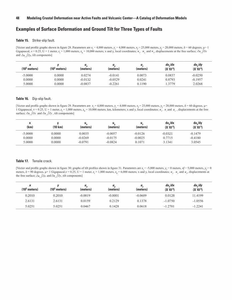
48 Modeling Crustal Deformation near Active Faults and Volcanic Center—A Catalog of Deformation Models
Table 17. Tensile crack.
[Vector and profile graphs shown in figure 30; graphs of tilt profiles shown in figure 31. Parameters are xi = -5,000 meters, yi = 0 meters, xf = 5,000 meters, yf = 0 meters, δ = 90 degrees, µ= 1 Gigapascal,ν = 0.25, U = 1 meter, zt = 1,000 meters, zb = 6,000 meters; x and y, local coordinates; u ux y, and uz , displacements at the free surface; ∂ ∂u xz and ∂ ∂u yz , tilt components]
x (103 meters)
y (103 meters)
ux(meters)
uy(meters)
uz(meters)
duz/dx(X 10-5)
duz/dy(X 10-5)
0.2010 0.2010 -0.0019 -0.0001 -0.0609 0.0128 11.4199 2.6131 2.6131 0.0159 0.2129 0.1378 -1.0750 -1.0556 5.0251 5.0251 0.0467 0.1428 0.0618 -1.2701 -1.2241
Table 15. Strike-slip fault.
[Vector and profile graphs shown in figure 28. Parameters are xi = 4,000 meters, yi = 4,000 meters, xf = 25,000 meters, yf = 20,000 meters, δ = 60 degrees, µ= 1 Gigapascal, ν = 0.25, U = 1 meter, zt = 1,000 meters, zb = 10,000 meters; x and y, local coordinates; u ux y, and uz , displacements at the free surface; ∂ ∂u xz and ∂ ∂u yz , tilt components]
x (103 meters)
y (103 meters)
ux(meters)
uy(meters)
uz(meters)
duz/dx(X 10-5)
duz/dy(X 10-5)
-5.0000 0.0000 0.0274 -0.0141 0.0073 0.0837 -0.02500.0000 0.0000 -0.0132 -0.0529 0.0241 0.8793 -0.19575.0000 0.0000 -0.0837 -0.2261 0.1190 1.3779 2.0268
Table 16. Dip-slip fault.
[Vector and profile graphs shown in figure 29. Parameters are xi = 4,000 meters, yi = 4,000 meters, xf = 25,000 meters, yf = 20,000 meters, δ = 60 degrees, µ= 1 Gigapascal, ν = 0.25, U = 1 meter, zt = 1,000 meters, zb = 10,000 meters; km, kilometers; x and y, local coordinates; u ux y, and uz , displacements at the free surface; ∂ ∂u xz and ∂ ∂u yz , tilt components]
x (km)
y(10 km)
ux(meters)
uy(meters)
uz(meters)
duz/dx(X 10-5)
duz/dy(X 10-5)
-5.0000 0.0000 0.0035 -0.0057 -0.0126 -0.0321 -0.14790.0000 0.0000 -0.0269 -0.0175 -0.0025 0.7715 -0.41805.0000 0.0000 -0.0791 -0.0824 0.1071 3.1341 3.0545
Examples of Surface Deformation and Ground Tilt for Three Types of Faults
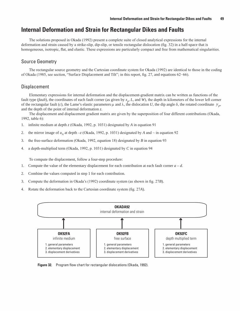
Internal Deformation and Strain for Rectangular Dikes and Faults 49
Internal Deformation and Strain for Rectangular Dikes and Faults The solutions proposed in Okada (1992) present a complete suite of closed analytical expressions for the internal
deformation and strain caused by a strike-slip, dip-slip, or tensile rectangular dislocation (fig. 32) in a half-space that is homogeneous, isotropic, flat, and elastic. These expressions are particularly compact and free from mathematical singularities.
Source GeometryThe rectangular source geometry and the Cartesian coordinate system for Okada (1992) are identical to those in the coding
of Okada (1985, see section, “Surface Displacement and Tilt”; in this report, fig. 27, and equations 62−66).
DisplacementElementary expressions for internal deformation and the displacement-gradient matrix can be written as functions of the
fault type (fault), the coordinates of each fault corner (as given by xp, L, and W), the depth in kilometers of the lower left corner of the rectangular fault (c), the Lame’s elastic parameters µ and λ, the dislocation U, the dip angle δ, the rotated coordinate yp, and the depth of the point of internal deformation z.
The displacement and displacement gradient matrix are given by the superposition of four different contributions (Okada, 1992, table 6):1. infinite medium at depth z (Okada, 1992, p. 1031) designated by A in equation 91
2. the mirror image of uA at depth –z (Okada, 1992, p. 1031) designated by A and ~ in equation 92
3. the free-surface deformation (Okada, 1992, equation 18) designated by B in equation 93
4. a depth-multiplied term (Okada, 1992, p. 1031) designated by C in equation 94
To compute the displacement, follow a four-step procedure:1. Compute the value of the elementary displacement for each contribution at each fault corner a – d.
2. Combine the values computed in step 1 for each contribution.
3. Compute the deformation in Okada’s (1992) coordinate system (as shown in fig. 27B).
4. Rotate the deformation back to the Cartesian coordinate system (fig. 27A).
Figure 32. Program flow chart for rectangular dislocations (Okada, 1992).
men12-7629_fig32
OKADA92internal deformation and strain
OK92FAinfinite medium
1. general parameters2. elementary displacement3. displacement derivatives
OK92FBfree surface
1. general parameters2. elementary displacement3. displacement derivatives
OK92FCdepth multiplied term
1. general parameters2. elementary displacement3. displacement derivatives
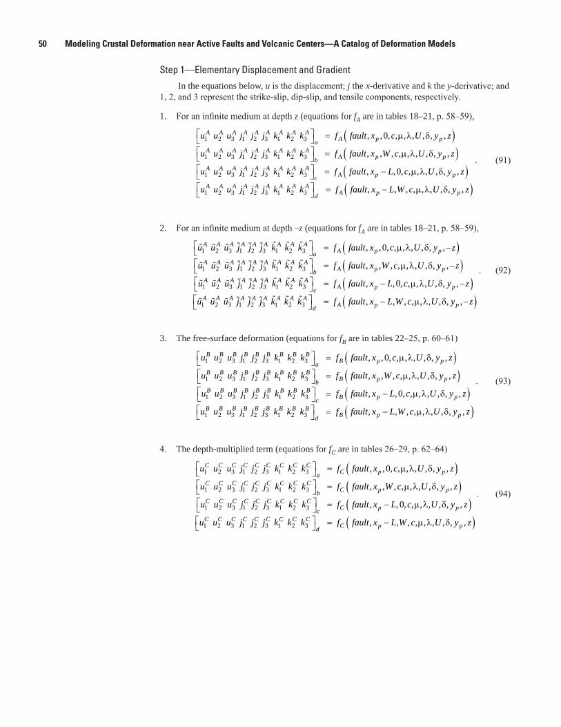
50 Modeling Crustal Deformation near Active Faults and Volcanic Centers—A Catalog of Deformation Models
Step 1—Elementary Displacement and GradientIn the equations below, u is the displacement; j the x-derivative and k the y-derivative; and
1, 2, and 3 represent the strike-slip, dip-slip, and tensile components, respectively.
1. For an infinite medium at depth z (equations for fA are in tables 18–21, p. 58–59),
( )( )
1 2 3 1 2 3 1 2 3
1 2 3 1 2 3 1 2 3
1 2 3 1 2 3 1 2 3
, ,0, , , , , , ,
, , , , , , , , ,
, ,0, ,
A A A A A A A A AA p pa
A A A A A A A A AA p pb
A A A A A A A A AA pc
u u u j j j k k k f fault x c U y z
u u u j j j k k k f fault x W c U y z
u u u j j j k k k f fault x L c
= µ λ δ = µ λ δ = − ( )
( )1 2 3 1 2 3 1 2 3
, , , , ,
, , , , , , , , ,
p
A A A A A A A A AA p pd
U y z
u u u j j j k k k f fault x L W c U y z
µ λ δ
= − µ λ δ
. (91)
2. For an infinite medium at depth –z (equations for fA are in tables 18–21, p. 58–59),
( )( )
1 2 3 1 2 3 1 2 3
1 2 3 1 2 3 1 2 3
1 2 3 1 2 3 1
, ,0, , , , , , ,
, , , , , , , , ,
A A A A A A A A AA p pa
A A A A A A A A AA p pb
A A A A A A A
u u u j j j k k k f fault x c U y z
u u u j j j k k k f fault x W c U y z
u u u j j j k k
= µ λ δ − = µ λ δ −
( )( )
2 3
1 2 3 1 2 3 1 2 3
, ,0, , , , , , ,
, , , , , , , , ,
A AA p pc
A A A A A A A A AA p pd
k f fault x L c U y z
u u u j j j k k k f fault x L W c U y z
= − µ λ δ − = − µ λ δ −
. (92)
3. The free-surface deformation (equations for fB are in tables 22–25, p. 60–61)
( )( )
1 2 3 1 2 3 1 2 3
1 2 3 1 2 3 1 2 3
1 2 3 1 2 3 1 2 3
, ,0, , , , , , ,
, , , , , , , , ,
, ,0
B B B B B B B B BB p pa
B B B B B B B B BB p pb
B B B B B B B B BB pc
u u u j j j k k k f fault x c U y z
u u u j j j k k k f fault x W c U y z
u u u j j j k k k f fault x L
= µ λ δ = µ λ δ = − ( )
( )1 2 3 1 2 3 1 2 3
, , , , , , ,
, , , , , , , , ,
p
B B B B B B B B BB p pd
c U y z
u u u j j j k k k f fault x L W c U y z
µ λ δ
= − µ λ δ
. (93)
4. The depth-multiplied term (equations for fC are in tables 26–29, p. 62–64)
( )( )
1 2 3 1 2 3 1 2 3
1 2 3 1 2 3 1 2 3
1 2 3 1 2 3 1 2 3
, ,0, , , , , , ,
, , , , , , , , ,
, ,0
C C C C C C C C CC p pa
C C C C C C C C CC p pb
C C C C C C C C CC pc
u u u j j j k k k f fault x c U y z
u u u j j j k k k f fault x W c U y z
u u u j j j k k k f fault x L
= µ λ δ = µ λ δ = − ( )
( )1 2 3 1 2 3 1 2 3
, , , , , , ,
, , , , , , , , ,
p
C C C C C C C C CC p pd
c U y z
u u u j j j k k k f fault x L W c U y z
µ λ δ
= − µ λ δ
. (94)
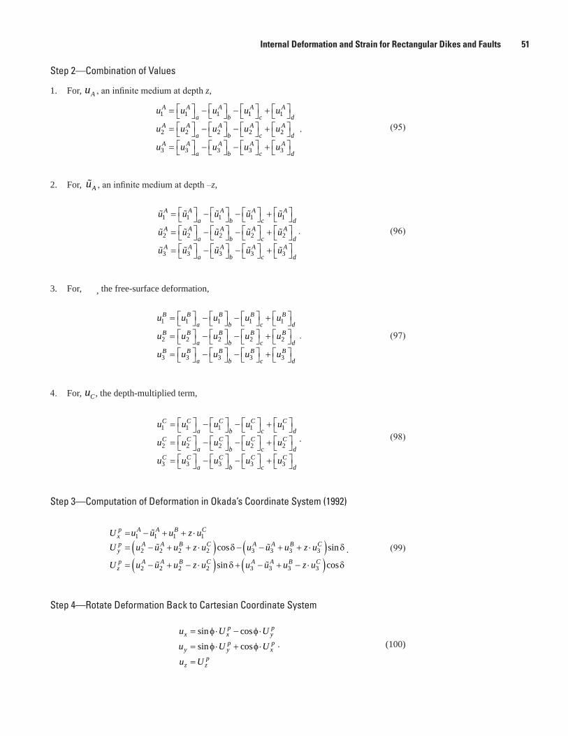
Internal Deformation and Strain for Rectangular Dikes and Faults 51
Step 2—Combination of Values
1. For, Au , an infinite medium at depth z,
1 1 1 1 1
2 2 2 2 2
3 3 3 3 3
A A A A Aa b c d
A A A A Aa b c d
A A A A Aa b c d
u u u u u
u u u u u
u u u u u
= − − + = − − + = − − +
. (95)
2. For, Au , an infinite medium at depth –z,
1 1 1 1 1
2 2 2 2 2
3 3 3 3 3
A A A A Aa b c d
A A A A Aa b c d
A A A A Aa b c d
u u u u u
u u u u u
u u u u u
= − − + = − − + = − − +
. (96)
3. For, , the free-surface deformation,
1 1 1 1 1
2 2 2 2 2
3 3 3 3 3
B B B B Ba b c d
B B B B Ba b c d
B B B B Ba b c d
u u u u u
u u u u u
u u u u u
= − − + = − − + = − − +
. (97)
4. For, Cu , the depth-multiplied term,
1 1 1 1 1
2 2 2 2 2
3 3 3 3 3
C C C C Ca b c d
C C C C Ca b c d
C C C C Ca b c d
u u u u u
u u u u u
u u u u u
= − − + = − − + = − − +
. (98)
Step 3—Computation of Deformation in Okada’s Coordinate System (1992)
( ) ( )( ) ( )
1 1 1 1
2 2 2 2 3 3 3 3
2 2 2 2 3 3 3 3
cos sin
sin cos
p A A B Cxp A A B C A A B Cy
p A A B C A A B Cz
U u u u z uU u u u z u u u u z u
U u u u z u u u u z u
= − + + ⋅
= − + + ⋅ δ − − + + ⋅ δ
= − + − ⋅ δ + − + − ⋅ δ
. (99)
Step 4—Rotate Deformation Back to Cartesian Coordinate System
sin cos
sin cos
p px x y
p py y x
pz z
u U Uu U Uu U
= φ⋅ − φ⋅
= φ⋅ + φ⋅
=
. (100)
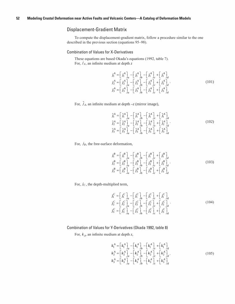
52 Modeling Crustal Deformation near Active Faults and Volcanic Centers—A Catalog of Deformation Models
Displacement-Gradient MatrixTo compute the displacement-gradient matrix, follow a procedure similar to the one
described in the previous section (equations 95–98).
Combination of Values for X-Derivatives These equations are based Okada’s equations (1992, table 7).For, jA, an infinite medium at depth z
1 1 1 1 1
2 2 2 2 2
3 3 3 3 3
A A A A Aa b c d
A A A A Aa b c d
A A A A Aa b c d
j j j j j
j j j j j
j j j j j
= − − + = − − + = − − +
. (101)
For, jA, an infinite medium at depth –z (mirror image),
1 1 1 1 1
2 2 2 2 2
3 3 3 3 3
A A A A Aa b c d
A A A A Aa b c d
A A A A Aa b c d
j j j j j
j j j j j
j j j j j
= − − + = − − + = − − +
. (102)
For, jB , the free-surface deformation,
1 1 1 1 1
2 2 2 2 2
3 3 3 3 3
B B B B Ba b c d
B B B B Ba b c d
B B B B Ba b c d
j j j j j
j j j j j
j j j j j
= − − + = − − + = − − +
. (103)
For, jC , the depth-multiplied term,
1 1 1 1 1
2 2 2 2 2
3 3 3 3 3
C C C C Ca b c d
C C C C Ca b c d
C C C C Ca b c d
j j j j j
j j j j j
j j j j j
= − − + = − − + = − − +
. (104)
Combination of Values for Y-Derivatives (Okada 1992, table 8)For, kA, an infinite medium at depth z,
1 1 1 1 1
2 2 2 2 2
3 3 3 3 3
A A A A Aa b c d
A A A A Aa b c d
A A A A Aa b c d
k k k k k
k k k k k
k k k k k
= − − + = − − + = − − +
. (105)
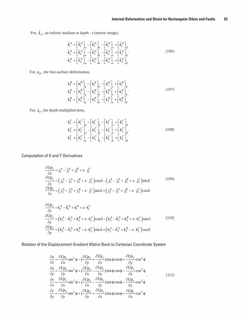
Internal Deformation and Strain for Rectangular Dikes and Faults 53
For, kA , an infinite medium at depth –z (mirror image),
1 1 1 1 1
2 2 2 2 2
3 3 3 3 3
A A A A Aa b c d
A A A A Aa b c d
A A A A Aa b c d
k k k k k
k k k k k
k k k k k
= − − + = − − + = − − +
. (106)
For, kB , the free-surface deformation,
1 1 1 1 1
2 2 2 2 2
3 3 3 3 3
B B B B Ba b c d
B B B B Ba b c d
B B B B Ba b c d
k k k k k
k k k k k
k k k k k
= − − + = − − + = − − +
. (107)
For, kC, the depth-multiplied term,
1 1 1 1 1
2 2 2 2 2
3 3 3 3 3
C C C C Ca b c d
C C C C Ca b c d
C C C C Ca b c d
k k k k k
k k k k k
k k k k k
= − − + = − − + = − − +
. (108)
Computation of X and Y Derivatives
( ) ( )( ) ( )
1 1 1 1
2 2 2 2 3 3 3 3
2 2 2 2 3 3 3 3
cos sin
sin cos
A A B Cx
y A A B C A A B C
A A B C A A B Cz
Upj j j z j
xUp
j j j z j j j j z jx
Up j j j z j j j j z jx
∂= − + + ⋅
∂∂
= − + + ⋅ δ − − + + ⋅ δ∂
∂= − + − ⋅ δ + − + − ⋅ δ
∂
. (109)
( ) ( )( ) ( )
1 1 1 1
2 2 2 2 3 3 3 3
2 2 2 2 3 3 3 3
cos sin
sin cos
A A B Cx
y A A B C A A B C
A A B C A A B Cz
Upk k k z k
yUp
k k k z k k k k z ky
Up k k k z k k k k z ky
∂= − + + ⋅
∂∂
= − + + ⋅ δ − − + + ⋅ δ∂
∂= − + − ⋅ δ + − + − ⋅ δ
∂
. (110)
Rotation of the Displacement-Gradient Matrix Back to Cartesian Coordinate System
2 2
2 2
2 2
2
sin ( )sin cos cos
sin ( )sin cos cos
sin ( )sin cos cos
sin ( )sin cos
y yx x
y yx x
y yx x
y yx
Up UpUp Upux x y x y
Up UpUp Upuy y x y x
Up UpUp Upvx x x y y
Up UpUp Upvy y y x
φ φ φ φ
φ φ φ φ
φ
∂ ∂∂ ∂∂= − + +
∂ ∂ ∂ ∂ ∂∂ ∂∂ ∂∂
= + − −∂ ∂ ∂ ∂ ∂
∂ ∂∂ ∂∂= + − −
∂ ∂ ∂ ∂ ∂∂ ∂∂
φ φ
∂∂= + + +
∂ ∂ ∂ ∂
φ
φ φ φ 2cosx
x∂φ
. (111)
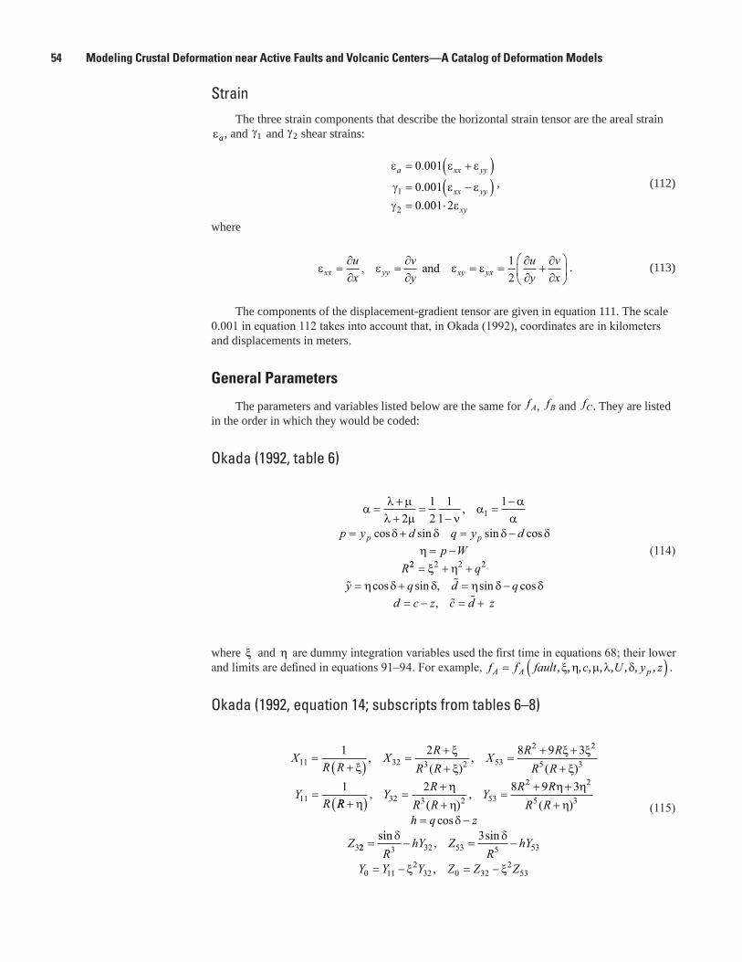
54 Modeling Crustal Deformation near Active Faults and Volcanic Centers—A Catalog of Deformation Models
StrainThe three strain components that describe the horizontal strain tensor are the areal strain
εa , and γ1 and γ2 shear strains:
ε ε ε
γ ε εγ ε
a xx yy
xx yy
xy
= +( )= −( )= ⋅
0 001
0 0010 001 2
1
2
.
.
.
, (112)
where
ε ε ε εxx yy xy yxux
vy
uy
vx
=∂∂
=∂∂
= =∂∂
+∂∂
, and 1
2. (113)
The components of the displacement-gradient tensor are given in equation 111. The scale 0.001 in equation 112 takes into account that, in Okada (1992), coordinates are in kilometers and displacements in meters.
General Parameters
The parameters and variables listed below are the same for fA, fB and fC. They are listed in the order in which they would be coded:
Okada (1992, table 6)
αλ µλ µ ν
ααα
δ δ δ δη
=++
=−
=−
= + = −= −
212
11
11,
cos sin sin cosp y d q y dp W
R
p p
22 2 2 2= + += + = −
= − = +
ξ ηη δ δ η δ δ
qy q d q
d c z c d z
cos sin , sin cos,
(114)
where x and η are dummy integration variables used the first time in equations 68; their lower and limits are defined in equations 91−94. For example, f f fault c U y zA A p= ( ), , , , , , , , ,ξ η µ λ δ .
Okada (1992, equation 14; subscripts from tables 6–8)
XR R
YR
X RR R
X R RR R11
11
32 3 2 53
2 2
5 31
1
2 8 9 3=
+( )
=
=++
=+ +
+ξξξ
ξ ξξ
,( )
,( )
RRh q z
Y RR R
Y R RR R
Z
+( )= −
=++
=+ +
+ηδ
ηη
η ηη
,
cos( )
,( )32 3 2 53
2 2
5 3
3
2 8 9 3
22 3 32 53 5 53
0 112
32 0 322
53
3= − = −
= − = −
sin , sin
,
δ δ
ξ ξR
hY ZR
hY
Y Y Y Z Z Z
(115)
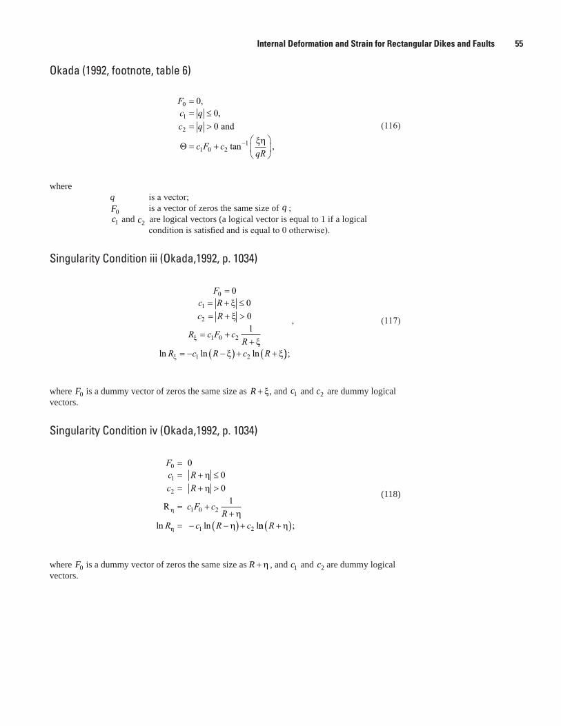
Internal Deformation and Strain for Rectangular Dikes and Faults 55
Okada (1992, footnote, table 6)
Fc qc q
c F cqR
0
1
2
1 0 21
000
== ≤= >
= +
−
,,
tan ,
and
Θξη
(116)
where q is a vector; F0 is a vector of zeros the same size of q ; c1 and c2 are logical vectors (a logical vector is equal to 1 if a logical
condition is satisfied and is equal to 0 otherwise).
Singularity Condition iii (Okada,1992, p. 1034)
Fc Rc R
R c F cR
R c R c R
0
1
2
1 0 2
1 2
0001
== + ≤= + >
= ++
= − −( ) + +(
ξξ
ξξ ξ
ξ
ξln ln ln ));
, (117)
where F0 is a dummy vector of zeros the same size as R + ξ, and c1 and c2 are dummy logical vectors.
Singularity Condition iv (Okada,1992, p. 1034)
Fc Rc R
c F cR
R c R c
0
1
2
1 0 2
1 2
000
1
== + ≤= + >
= ++
= − −( ) +
ηη
ηη
η
η
R
ln ln lnn ;R +( )η
(118)
where F0 is a dummy vector of zeros the same size as R + η , and c1 and c2 are dummy logical vectors.
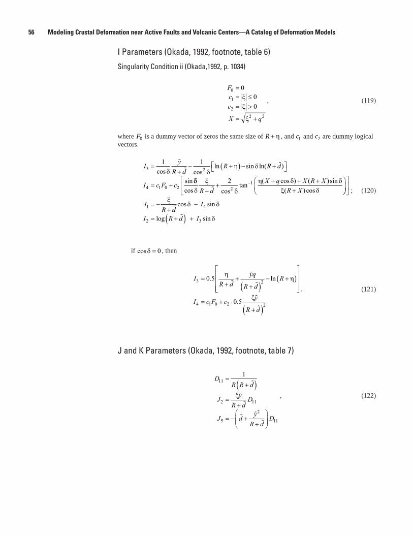
56 Modeling Crustal Deformation near Active Faults and Volcanic Centers—A Catalog of Deformation Models
I Parameters (Okada, 1992, footnote, table 6)
Singularity Condition ii (Okada,1992, p. 1034)
Fcc
X q
0
1
22 2
000
== ≤= >
= +
ξξ
ξ
, (119)
where F0 is a dummy vector of zeros the same size of R + η , and c1 and c2 are dummy logical vectors.
I yR d
R R d
I c F c
3 2
4 1 0 2
1 1=
+− +( ) − +
= +
cos cosln sin ln( )
sinδ δ
η δ
δδδ
ξδ
η δ δξ δcos cos
tan ( cos ) ( )sin( ) cosR d
X q X R XR X+
++ + +
+
−
22
1
= −+
−
= +( ) +
IR
I
I R Idd
1 4
2 3
ξδ δ
δ
cos sin
log sin
; (120)
if cosδ = 0 , then
IR d
yq
R dR
I c F c y
R
3 2
4 1 0 2
0 5
0 5
=+
++( )
− +( )
= + ⋅
. ln
.
ηη
ξ
++( )d 2
. (121)
J and K Parameters (Okada, 1992, footnote, table 7)
DR R d
J yR d
D
J d yR d
D
11
2 11
5
2
11
1=
+( )=
+
= − ++
ξ , (122)
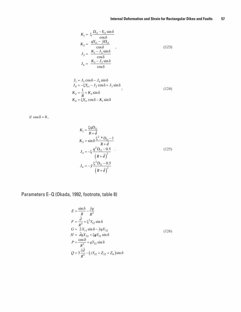
Internal Deformation and Strain for Rectangular Dikes and Faults 57
11 111
11 113
1 23
3 56
sin
cos
cos
sin
cossin
cos
D YK
qY yDK
K JJ
K JJ
− δ= x
δ−
=δ
− δ=
δ− δ
=δ
, (123)
1 5 6
4 11 2 3
2 3
4 11 1
cos sincos sin
1 sin
cos sin
J J JJ Y J J
K KR
K Y K
= δ − δ= −x − δ + δ
= + δ
= x δ − δ
; (124)
if cosδ = 0 ,
( )
( )
111
211
3
211
3 2
211
6 2
.* 1sin
0.5
0.5
qDKR d
DKR d
q DJR d
DJ yR d
x=
+x −
= δ+−
= −x+
x −= −
+
. (125)
Parameters E–Q (Okada, 1992, footnote, table 8)
ER
yqR
F dR
Y
yd
G X qXH qX
= −
= +
= −= +
sin
sin
sin
δ
ξ δ
δξ
3
32
32
11 32
32
2 qqY
PR
qY
Q cdR
zY Z Z
32
3 32
5 32 32 03
sincos sin
sin
δδ
δ
δ
= +
= − + +( )
(126)
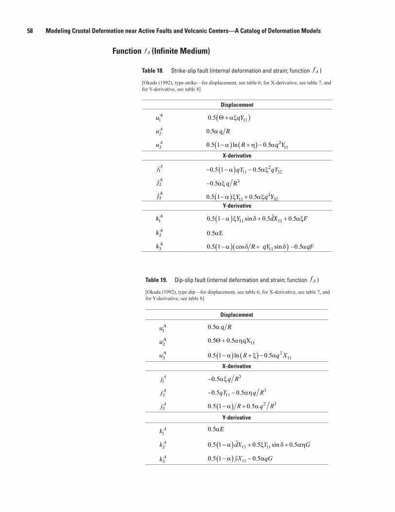
58 Modeling Crustal Deformation near Active Faults and Volcanic Centers—A Catalog of Deformation Models
Table 18. Strike-slip fault (internal deformation and strain; function fA )
[Okada (1992), type strike—for displacement, see table 6; for X-derivative, see table 7, and for Y-derivative, see table 8]
Displacement
1Au
( )110.5 qYΘ + αx
uA2 0.5 q Rα
uA3 ( ) ( ) 2110.5 1 ln 0.5R q Y− α + η − α
X-derivative
j A1 − −( ) −0 5 1 0 5112
32. .α αξqY qY
2Aj 30.5 q R− αx
3Aj ( ) 2
11 320.5 1 0.5Y q Y− α x + αxY-derivative
1Ak ( ) 11 11 0.5 1 sin 0.5 0.5 Y dX F− α x δ + + αx
2Ak 0.5 E α
3Ak ( )( )11 0.5 1 cos sin 0.5 R qY qF− α δ + δ − α
Table 19. Dip-slip fault (internal deformation and strain; function fA )
[Okada (1992), type dip—for displacement, see table 6; for X-derivative, see table 7, and for Y-derivative, see table 8]
Displacement
1Au 0.5 q Rα
2Au 110.5 0.5 qXΘ + αη
3Au 0 5 1 0 5 2
11. ln .−( ) +( ) −α ξ αR q XX-derivative
j A1 −0 5 3. αξq R
j A2 − −0 5 0 5113. .qY q Rαη
j A3 0 5 1 0 5 2 3. .−( ) +α αR q R
Y-derivative
k A1 0 5. αE
k A2 0 5 1 0 5 0 511 11. . sin .−( ) + +α ξ δ αηdX Y G
k A3 0 5 1 0 511. .−( ) −α αyX qG
Function fA (Infinite Medium)
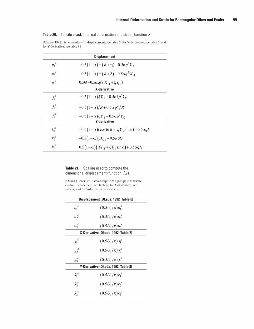
Internal Deformation and Strain for Rectangular Dikes and Faults 59
Table 21. Scaling used to compute the dimensional displacement (function fA ).
[Okada (1992), i=1: strike-slip; i=2: dip-slip; i=3: tensile e—for displacement, see table 6; for X-derivative, see table 7, and for Y-derivative, see table 8]
Displacement (Okada, 1992; Table 6)
uA1 0 5 1. U uiAπ( )
uA2 0 5 2. U uiAπ( )
uA3 0 5 3. U uiAπ( )
X-Derivative (Okada, 1992; Table 7)
j A1 0 5 1. U jiAπ( )
j A2 0 5 2. U jiAπ( )
j A3 0 5 3. U jiAπ( )
Y-Derivative (Okada, 1992; Table 8)
k A1 0 5 1. U kiAπ( )
k A2 0 5 2. U kiAπ( )
k A3 0 5 3. U kiAπ( )
Table 20. Tensile crack (internal deformation and strain; function fA )
[Okada (1992), type tensile—for displacement, see table 6; for X-derivative, see table 7, and for Y-derivative, see table 8]
Displacement
uA1 − −( ) +( ) −0 5 1 0 5 211. ln .α η αR q Y
uA2 − −( ) +( ) −0 5 1 0 5 211. ln .α ξ αR q X
uA3 ( )11 110.5 0.5 q X YΘ− α η + x
X-derivative
j A1 − −( ) +0 5 1 0 5112
32. .α ξ αξY q Y
j A2 − −( ) +0 5 1 0 5 2 3. .α αR q R
j A3 − −( ) −0 5 1 0 5113
32. .α αqY q YY-derivative
k A1 − −( ) +( ) −0 5 1 0 511. cos sin . �α δ δ αR qY qF
k A2 ( ) 11 0.5 1 0.5 yX qG− − α − α
k A3 0 5 1 0 511 11. sin .−( ) +( ) +α ξ δ αdX Y qH
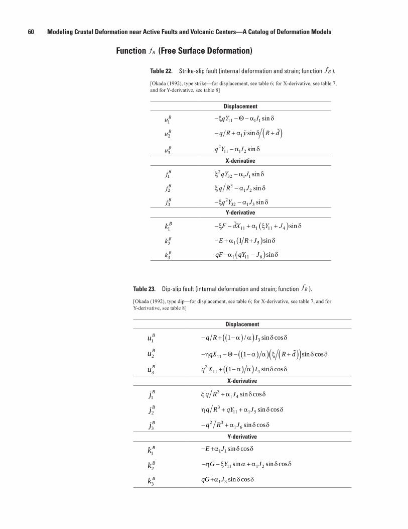
60 Modeling Crustal Deformation near Active Faults and Volcanic Centers—A Catalog of Deformation Models
Table 22. Strike-slip fault (internal deformation and strain; function fB ).
[Okada (1992), type strike—for displacement, see table 6; for X-derivative, see table 7, and for Y-derivative, see table 8]
Displacement
uB1 − − −ξ α δqY I11 1 1Θ sin
uB2 − + +( )q R y R dα δ1 sin
uB3 q Y I211 1 2−α δsin
X-derivative
jB1 ξ α δ232 1 1qY J− sin
jB2 ξ α δq R J31 2− sin
jB3 − −ξ α δq Y J232 1 3 sin
Y-derivative
kB1 − − + +( )ξ α ξ δF dX Y J
11 1 11 4 sin
kB2 ( )1 51 sinE R J− + α + δ
kB3 ( )1 11 6 sinqF qY J−α − δ
Table 23. Dip-slip fault (internal deformation and strain; function fB ).
[Okada (1992), type dip—for displacement, see table 6; for X-derivative, see table 7, and for Y-derivative, see table 8]
Displacement
1Bu ( )( ) 31 / sin cos q R I− + − α α δ δ
2Bu ( )( ) ( )( )11 1 sin cosqX R d−η − Θ − − α α x + δ δ
3Bu ( )( )2
11 41 sin cosq X I+ − α α δ δ
X-derivative
1Bj 3
1 4 sin cosq R Jx + α δ δ
2Bj 3
11 1 5 sin cosq R qY Jη + + α δ δ
3Bj 2 3
1 6 sin cosq R J− + α δ δ
Y-derivative
1Bk 1 1 sin cos E J− +α δ δ
2Bk 11 1 2 sin sin cosG Y J−η − x α + α δ δ
3Bk 1 3 sin cosqG J+α δ δ
Function fB (Free Surface Deformation)
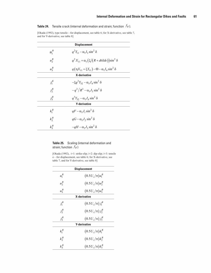
Internal Deformation and Strain for Rectangular Dikes and Faults 61
Table 25. Scaling (internal deformation and strain; function fB )
[Okada (1992), i=1: strike-slip; i=2: dip-slip; i=3: tensile e—for displacement, see table 6; for X-derivative, see table 7, and for Y-derivative, see table 8]
Displacement
uB1 0 5 1. U uiBπ( )
uB2 0 5 2. U uiBπ( )
uB3 0 5 3. U uiBπ( )
X-derivative
jB1 0 5 1. U jiBπ( )
jB2 0 5 2. U jiBπ( )
jB3 0 5 3. U jiBπ( )
Y-derivative
kB1 0 5 1. U kiBπ( )
kB2 0 5 2. U kiBπ( )
kB3 0 5 3. U kiBπ( )
Table 24. Tensile crack (internal deformation and strain; function fB ).
[Okada (1992), type tensile—for displacement, see table 6; for X-derivative, see table 7, and for Y-derivative, see table 8]
Displacement
uB1 q Y I211 1 3
2−α δsin
uB2 q X R dtilde211 1
2+ +( )( )α ξ δsin
uB3 q X Y Iη ξ α δ11 11 1 42+( ) − −Θ sin
X-derivative
jB1 − −ξ α δq Y J232 1 4
2sin
jB2 − −q R J2 31 5
2α δsin
jB3 q Y J332 1 6
2−α δsin
Y-derivative
kB1 qF J−α δ1 12sin
kB2 qG J−α δ1 22sin
kB3 − −qH Jα δ1 32sin
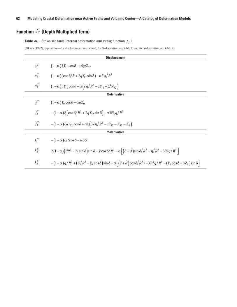
62 Modeling Crustal Deformation near Active Faults and Volcanic Center—A Catalog of Deformation Models
Table 26. Strike-slip fault (internal deformation and strain; function fC ).
[Okada (1992), type strike—for displacement, see table 6; for X-derivative, see table 7, and for Y-derivative, see table 8]
Displacement
uC1 1 11 32−( ) −α ξ δ αξY qZcos
uC2 1 2 113−( ) +( ) −α δ δ αcos sinR qY c q R
uC3 1 113
112
32−( ) − − +( )α δ α η ξqY c R zY Zcos
X-derivative
jC1 1 0 0−( ) −α δ αY qZcos
jC2 − −( ) +( ) +1 2 3332
5α ξ δ δ α ξcos sinR qY c q R
jC3 − −( ) + − − −( )1 3325
32 32 0α ξ δ αξ ηqY c R zY Z Zcos
Y-derivative
kC1 − −( ) −1 α ξ δ αξP Qcos
kC2 2 1 330
3 3 3−( ) −( ) − − +( ) − −α δ δ δ α δ η
dR Y y R c d R R cy qsin sin cos sin RR5
kC3 − −( ) + −( ) + +( ) + −1 33 30
3 50α δ δ α δq R y R Y c d R cd q R Y
cos sin cos / cosδδ δ+( )
qZ0 sin
Function fC (Depth Multiplied Term)
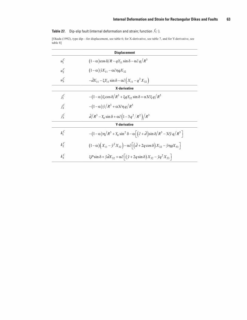
Internal Deformation and Strain for Rectangular Dikes and Faults 63
Table 27. Dip-slip fault (internal deformation and strain; function fC ).
[Okada (1992), type dip—for displacement, see table 6; for X-derivative, see table 7, and for Y-derivative, see table 8]
Displacement
uC1 1 113−( ) − −α δ δ αcos sinR qY c q R
uC2 1 11 32−( ) −α α η yX c qX
uC3 − − − −( )
dX Y c X q X11 11 112
32ξ δ αsin
X-derivative
jC1 − −( ) + +1 3332
5α ξ δ ξ δ α ξcos sinR qY c q R
jC2 − −( ) +1 33 5α α η y R c q R
jC3
d R Y c q R R30
2 2 31 3− + −( )sin δ α
Y-derivative
kC1 − −( ) + − +( ) −
1 33
02 3 5α η α δδR Y c d R cy q Rsin sin
kC2 1 2112
32 32 53−( ) −( ) − +( ) −
α α δ ηX y X c d q X y qX
cos
kC3 ξ δ α δP ydX c y q X yq Xsin sin+ + +( ) −
32 322
532
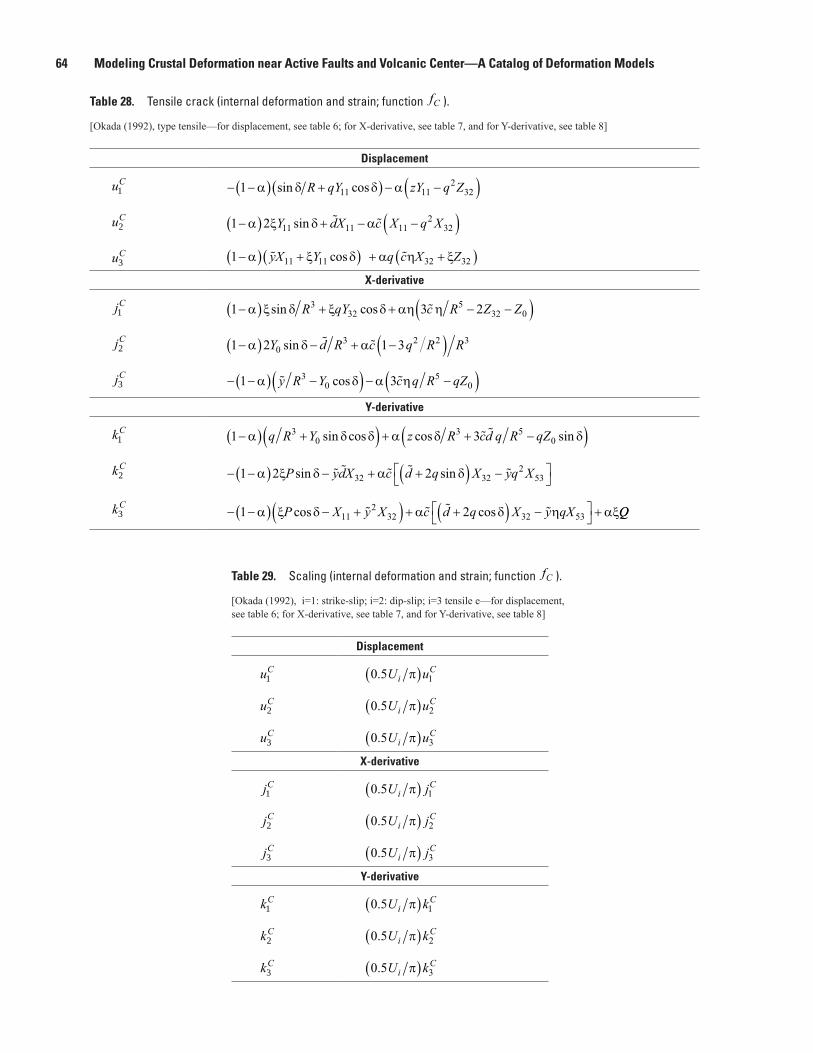
64 Modeling Crustal Deformation near Active Faults and Volcanic Center—A Catalog of Deformation Models
Table 29. Scaling (internal deformation and strain; function fC ).
[Okada (1992), i=1: strike-slip; i=2: dip-slip; i=3 tensile e—for displacement, see table 6; for X-derivative, see table 7, and for Y-derivative, see table 8]
Displacement
uC1 0 5 1. U uiCπ( )
uC2 0 5 2. U uiCπ( )
uC3 0 5 3. U uiCπ( )
X-derivative
jC1 0 5 1. U jiCπ( )
jC2 0 5 2. U jiCπ( )
jC3 0 5 3. U jiCπ( )
Y-derivative
kC1 0 5 1. U kiCπ( )
kC2 0 5 2. U kiCπ( )
kC3 0 5 3. U kiCπ( )
Table 28. Tensile crack (internal deformation and strain; function fC ).
[Okada (1992), type tensile—for displacement, see table 6; for X-derivative, see table 7, and for Y-derivative, see table 8]
Displacement
uC1 − −( ) +( ) − −( )1 11 112
32α δ δ αsin cosR qY zY q Z
uC2 1 2 11 11 112
32−( ) + − −( )α ξ δ αY dX c X q Xsin
uC3 1 11 11 32 32−( ) +( ) + +( )α ξ δ α η ξ yX Y q c X Zcos
X-derivative
jC1 1 3 2332
532 0−( ) + + − −( )α ξ δ ξ δ αη ηsin cosR qY c R Z Z
jC2 1 2 1 303 2 2 3−( ) − + −( )α δ αY d R c q R Rsin
jC3 − −( ) −( ) − −( )1 330
50α δ α η y R Y c q R qZcos
Y-derivative
kC1 1 330
3 50−( ) +( ) + + −( )α δ δ α δ δq R Y z R cd q R qZsin cos cos sin
kC2 − −( ) − + +( ) −
1 2 232 32
253α ξ δ α δP ydX c d q X yq Xsin sin
kC3 − −( ) − +( ) + +( ) −
+1 211
232 32 53α ξ δ α δ η αξP X y X c d q X y qXcos cos
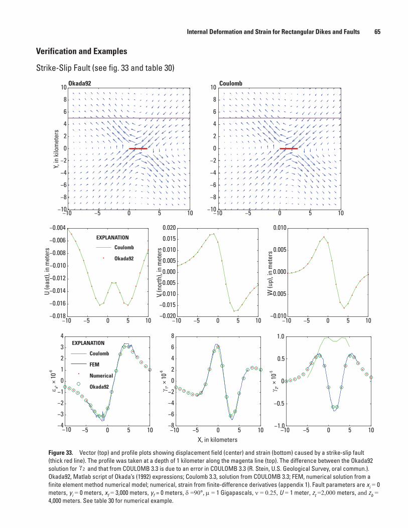
Internal Deformation and Strain for Rectangular Dikes and Faults 65
Verification and Examples
Strike-Slip Fault (see fig. 33 and table 30)
men12-7629_fig33
−10 −5 0 5 10−10
−8
−6
−4
−2
0
2
4
6
8
10
−10
−8
−6
−4
−2
0
2
4
6
8
10Okada92
Y, in
kilo
met
ers
−10 −5 0 5 10
Coulomb
−10 −5 0 5 10−0.018
−0.016
−0.014
−0.012
−0.010
−0.008
−0.006
−0.004
U (e
ast),
in m
eter
s
−10 −5 0 5 10−0.020
−0.015
−0.010
−0.005
0.000
0.005
0.010
0.015
0.020
V (n
orth
), in
met
ersCoulomb
Okada92
−10 −5 0 5 10−0.010
−0.005
0.000
0.005
0.010
W (u
p), i
n m
eter
s
−10 −5 0 5 10−4
−3
−2
−1
0
1
2
3
4
ε a, ×
10-6
−10 −5 0 5 10−8
−6
−4
−2
0
2
4
6
8
X, in kilometers
γ 1, ×
10-6
Coulomb
FEM
Numerical
Okada92
−10 −5 0 5 10−1.0
−0.5
0
0.5
1.0
γ 2, ×
10-5
EXPLANATION
EXPLANATION
Figure 33. Vector (top) and profile plots showing displacement field (center) and strain (bottom) caused by a strike-slip fault (thick red line). The profile was taken at a depth of 1 kilometer along the magenta line (top). The difference between the Okada92 solution for γ2 and that from COULOMB 3.3 is due to an error in COULOMB 3.3 (R. Stein, U.S. Geological Survey, oral commun.). Okada92, Matlab script of Okada’s (1992) expressions; Coulomb 3.3, solution from COULOMB 3.3; FEM, numerical solution from a finite element method numerical model; numerical, strain from finite-difference derivatives (appendix 1). Fault parameters are xi = 0 meters, yi = 0 meters, xf = 3,000 meters, yf = 0 meters, δ =90°, µ = 1 Gigapascals, ν = 0.25, U = 1 meter, zt =2,000 meters, and zb = 4,000 meters. See table 30 for numerical example.
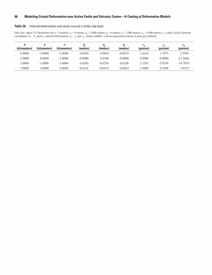
66 Modeling Crustal Deformation near Active Faults and Volcanic Center—A Catalog of Deformation Models
Table 30. Internal deformation and strain around a strike-slip fault.
[See also figure 33. Parameters are xi = 0 meters, yi = 0 meters, xf = 3,000 meters; yf = 0 meters; zt = 2,000 meters; zb = 4,000 meters; x, y and z, local Cartesian coordinates; u ux y, and uz , internal deformation; ε γa , 1 and γ2 , strain; strainµ , a strain expressed in terms of parts per million]
x (kilometers)
y(kilometers)
z(kilometers)
ux(meters)
uy(meters)
uz(meters)
εa(μstrain)
γ1(μstrain)
γ2(μstrain)
-5.0000 -5.0000 -1.0000 0.0103 0.0092 -0.0014 1.6162 1.1973 2.9945-1.0000 0.0000 -1.0000 -0.0000 0.0186 -0.0000 0.0000 0.0000 -27.56463.0000 -1.0000 -1.0000 0.0283 -0.0259 0.0230 2.1363 -5.9239 -14.7870
7.0000 5.0000 -1.0000 -0.0116 -0.0113 -0.0023 1.9409 0.3598 3.8515
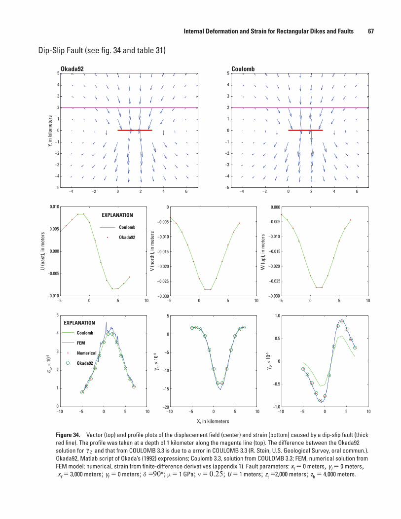
Internal Deformation and Strain for Rectangular Dikes and Faults 67
Dip-Slip Fault (see fig. 34 and table 31)
men12-7629_fig34
−4 −2 0 2 4 6−5
−4
−3
−2
−1
0
1
2
3
4
5
−5
−4
−3
−2
−1
0
1
2
3
4
5Okada92
Y, in
kilo
met
ers
−4 −2 0 2 4 6
Coulomb
−5 0 5 10−0.010
−0.005
0.000
0.005
0.010
U (e
ast),
in m
eter
s
−5 0 5 10−0.030
−0.025
−0.020
−0.015
−0.010
−0.005
0
V (n
orth
), in
met
ers
−5 0 5 10−0.030
−0.025
−0.020
−0.015
−0.010
−0.005
0.000
W (u
p), i
n m
eter
s
−10 −5 0 5 100
1
2
3
4
5
ε a, ×
10-6
−10 −5 0 5 10−20
−15
−10
−5
0
5
X, in kilometers
γ 1, ×
10-6
−10 −5 0 5 10−1.0
−0.5
0
0.5
1.0
γ 2, ×
10-5
Coulomb
FEM
Numerical
Okada92
Coulomb
Okada92
EXPLANATION
EXPLANATION
Figure 34. Vector (top) and profile plots of the displacement field (center) and strain (bottom) caused by a dip-slip fault (thick red line). The profile was taken at a depth of 1 kilometer along the magenta line (top). The difference between the Okada92 solution for γ2 and that from COULOMB 3.3 is due to a error in COULOMB 3.3 (R. Stein, U.S. Geological Survey, oral commun.). Okada92, Matlab script of Okada’s (1992) expressions; Coulomb 3.3, solution from COULOMB 3.3; FEM, numerical solution from FEM model; numerical, strain from finite-difference derivatives (appendix 1). Fault parameters: xi = 0 meters, yi = 0 meters, xf = 3,000 meters; yf = 0 meters; δ =90°; µ = 1 GPa; ν = 0.25; U = 1 meters; zt =2,000 meters; zb = 4,000 meters.

68 Modeling Crustal Deformation near Active Faults and Volcanic Center—A Catalog of Deformation Models
Table 31. Internal deformation and strain around a dip-slip fault.
[See figure 34. Parameters are xi = 0 meters, yi = 0 meters, xf = 3,000 meters; yf = 0 meters; δ =90°; μ= 1 GPa; ν = 0.25; U = 1 meters; zt =2,000 meters; zb = 4,000 meters; x, y and z, local Cartesian coordinates; u ux y, and uz, internal deformation; ε γa , 1 and γ2 , strain; strainµ , a strain expressed in terms of parts per million]
x (kilometers)
y (kilometers)
z(kilometers )
ux(meters)
uy(meters)
uz(meters)
εa(μstrain)
γ1(μstrain)
γ2(μstrain)
-5.0000 -5.0000 -1.0000 0.0041 -0.0038 0.0024 -0.7843 -1.0461 -1.9073-1.0000 0.0000 -1.0000 0.0000 -0.0195 0.0000 -0.0000 0.0000 5.94633.0000 -1.0000 -1.0000 0.0177 -0.0486 0.0653 5.7981 0.4789 26.5485
7.0000 5.0000 -1.0000 0.0051 -0.0056 -0.0036 1.0556 0.8267 2.9135
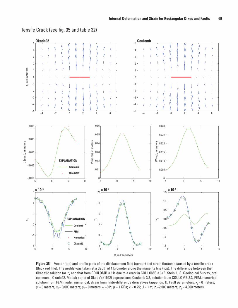
Internal Deformation and Strain for Rectangular Dikes and Faults 69
Tensile Crack (see fig. 35 and table 32)
men12-7629_fig35
−4 −2 0 2 4 6−5
−4
−3
−2
−1
0
1
2
3
4
5Okada92
Y, in
kilo
met
ers
−4 −2 0 2 4 6−5
−4
−3
−2
−1
0
1
2
3
4
5Coulomb
−5 0 5 10−0.010
−0.005
0.000
0.005
0.010
U (e
ast),
in m
eter
s
−5 0 5 100
0.01
0.02
0.03
0.04
0.05
0.06
V (n
orth
), in
met
ers
−5 0 5 100
0.005
0.010
0.015
0.020
0.025
0.030
W (u
p), i
n m
eter
s
−5 0 5 10−4
−3
−2
−1
0
1× 10⁻⁶
ε a
−5 0 5 10−5
0
5
10
15
20× 10−6
X, in kilometers
γ 1
Coulomb
FEM
Numerical
Okada92
Coulomb
Okada92
−5 0 5 10−1.5
−1.0
−0.5
0.0
0.5
1.0
1.5× 10⁻⁵
γ 2EXPLANATION
EXPLANATION
Figure 35. Vector (top) and profile plots of the displacement field (center) and strain (bottom) caused by a tensile crack (thick red line). The profile was taken at a depth of 1 kilometer along the magenta line (top). The difference between the Okada92 solution for γ2 and that from COULOMB 3.3 is due to a error in COULOMB 3.3 (R. Stein, U.S. Geological Survey, oral commun.). Okada92, Matlab script of Okada’s (1992) expressions; Coulomb 3.3, solution from COULOMB 3.3; FEM, numerical solution from FEM model; numerical, strain from finite-difference derivatives (appendix 1). Fault parameters: xi = 0 meters, yi = 0 meters, xf = 3,000 meters; yf = 0 meters; δ =90°; µ = 1 GPa; ν = 0.25; U = 1 m; zt =2,000 meters; zb = 4,000 meters.
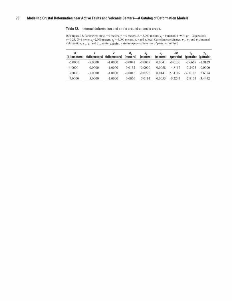
70 Modeling Crustal Deformation near Active Faults and Volcanic Centers—A Catalog of Deformation Models
Table 32. Internal deformation and strain around a tensile crack.
[See figure 35. Parameters are xi = 0 meters, yi = 0 meters, xf = 3,000 meters; yf = 0 meters; δ=90°; μ=1 Gigapascal; ν= 0.25, U=1 meter, zt=2,000 meters; zb = 4,000 meters. x, y and z, local Cartesian coordinates; u ux y, and uz , internal deformation; ε γa , 1 and γ2 , strain; strainµ , a strain expressed in terms of parts per million]
x (kilometers)
y (kilometers)
z(kilometers)
ux(meters)
uy(meters)
uz(meters)
εa(μstrain)
γ1(μstrain)
γ2(μstrain)
-5.0000 -5.0000 -1.0000 -0.0041 -0.0079 0.0041 -0.0138 -2.6669 -1.9129-1.0000 0.0000 -1.0000 0.0152 -0.0000 -0.0058 14.8157 -7.2473 -0.00003.0000 -1.0000 -1.0000 -0.0013 -0.0296 0.0141 27.4109 -32.0105 2.6374
7.0000 5.0000 -1.0000 0.0056 0.0114 0.0055 -0.2245 -2.9155 -3.4452
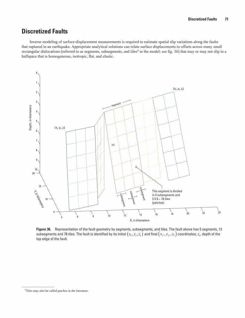
Discretized Faults 71
Discretized FaultsInverse modeling of surface-displacement measurements is required to estimate spatial slip variations along the faults
that ruptured in an earthquake. Appropriate analytical solutions can relate surface displacements to offsets across many small rectangular dislocations (referred to as segments, subsegments, and tiles4 in the model; see fig. 36) that may or may not slip in a halfspace that is homogeneous, isotropic, flat, and elastic.
4Tiles may also be called patches in the literature.
Figure 36. Representation of the fault geometry by segments, subsegments, and tiles. The fault above has 5 segments, 13 subsegments and 78 tiles. The fault is identified by its initial x y zi i t, ,( ) and final x y zf f t, ,( ) coordinates; zt , depth of the top edge of the fault.
men12-7629_fig36
4 6 8 10 12 14 16 18 20 22 245
10
15
20
0
1
2
3
4
5
6
7
8
9
10
X, in kilometers
Dept
h, in
kilo
met
ers segment
tile
(xi, yi, zt)
(xf, yf, zt)
Y, in kilometers
subsegment
subsegment
subsegment
This segment is divided in 3 subsegments and 3 X 6 = 18 tiles (patches)
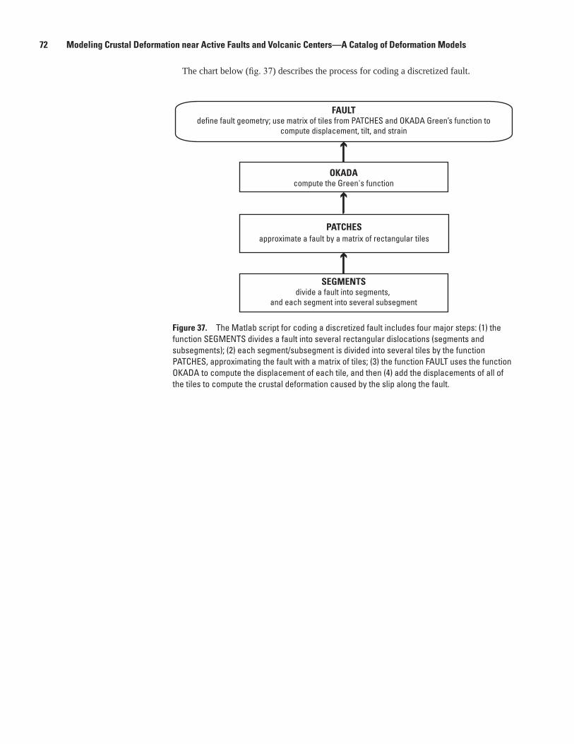
72 Modeling Crustal Deformation near Active Faults and Volcanic Centers—A Catalog of Deformation Models
The chart below (fig. 37) describes the process for coding a discretized fault.
men12-7629_fig37
SEGMENTSdivide a fault into segments,
and each segment into several subsegment
FAULTdefine fault geometry; use matrix of tiles from PATCHES and OKADA Green’s function to
compute displacement, tilt, and strain
PATCHESapproximate a fault by a matrix of rectangular tiles
OKADAcompute the Green's function
Figure 37. The Matlab script for coding a discretized fault includes four major steps: (1) the function SEGMENTS divides a fault into several rectangular dislocations (segments and subsegments); (2) each segment/subsegment is divided into several tiles by the function PATCHES, approximating the fault with a matrix of tiles; (3) the function FAULT uses the function OKADA to compute the displacement of each tile, and then (4) add the displacements of all of the tiles to compute the crustal deformation caused by the slip along the fault.
Discretized Faults 73
Fault Segments and Subsegments
Estimating the location, size, dip, orientation, and slip across multiple rectangular dislocations that may or may not slip is a numerically challenging task given the number of data points and the number of parameters required to estimate these dislocations. Information from the mapped fault trace can be used to constrain several parameters of the fault geometry, including the number of segments that could reasonably represent the fault trace at the surface:
L x x y yn
inf
ni
nf
n
N= −( ) + −( )
=∑ )
2 2
1
(127)
and
N =
length of fault tracewidth of segment
, (128)
where L is the length of the fault trace, ( , )x yni
ni and
( , )x ynf
nf are the initial and final points of the segment,
n is index of the nth segment, N is the number of segments, and is the ceiling function (fig. 36). The (x, y) coordinates of points of the grid
along the upper edge of each subsegment (figs. 36 and 38) are defined by
( )
( )
0 :1:f i
i n nn
ff f i n
n n n f in n
x xxx x S
Sxx x
yy y y yx x
−= +
−= + −
−
, (129)
where S is the total number of subsegments, and each subsegment’s initial and final point
( ) ( )( ) ( )
1: , 1: 2 : 1 , 2 : 1
i is sf fs s
x xx S y yy Sx xx S y yy S
= =
= + = +. (130)

74 Modeling Crustal Deformation near Active Faults and Volcanic Centers—A Catalog of Deformation Models
Tiles
Each subsegment (figs. 36 and 38) can be divided into several tiles following the steps described below. First, define three parameters:1. the subsegment at the initial (lower left) corner
x x z z
y y z z
isi
sb
st
isi
sb
st
0
0
= + −( )= − −( )
cot cos
cot sin
δ φ
δ φ, (131)
men12-7629_fig38
zt
zb
(xin, yi
n)(xf
n, yfn)
X
Y
Z (d
epth
)
tile p
(xip, yi
p, zbp)(xf
p, yfp, zbp)
(xip, yi
p, ztp)(xf
p, yfp, ztp)
(xis, yi
s, zts) (xfs, yf
s, zts)
(xis, yi
s, zbs)(xf
s, yfs, zbs)
subsegment s
segment n
Figure 38. Segment, subsegment, and tile geometry. x yi i,( ) , horizontal coordinates for the left corner of segments, subsegments, or tiles; x yf f,( ), horizontal coordinates for the right corner segments, subsegments, or tiles; zt , depth of the top edge of segments, subsegments or tiles; zb , depth of the bottom edge of segments, subsegments, or tiles; n, s or p, subindex for segments, subsegments, or tiles.
Discretized Faults 75
2. the subsegment at the final (lower right) corner
x x z z
y y z z
fsf
sb
st
fsf
sb
st
0
0
= + −( )= − −( )
cot cos
cot sin
δ φ
δ φ
, and (132)
3. the number of tiles P for each subsegment (the symbol is the ceiling function)
P =
height of subsegmentheight of tile
. (133)
Then, compute the coordinates of the grid of tiles at the initial (left) and final (right) side of each segment by using the formulas below:
1. grid along the depth
zz z P z z Pst
sb
st= + ( ) −( )0 1: : , (134)
2. grid along the left side of the segment
xx x x x zz z z z
yy y y y zz zi
isi i
sb
st
sb
ii
si i
sb
= + −( ) −( ) −( )= + −( ) −(
0 0
0 0 )) −( )z zst
sb
and (135)
3. grid along the right side of the segment
( )( ) ( )( )( ) ( )
0 0
0 0
f ff b t bf s s s s
f ff b t bf s s s s
xx x x x zz z z z
yy y y y zz z z z
= + − − −
= + − − −
. (136)
Finally, we define the tile at the top left corner (initial point), the tile at the top right corner (final point), and the tiles at the top and bottom as
( ) ( )( ) ( )
( ) ( )
1: 1:
1: 1:
1: 2 : 1
i ip i p if fp f p ft bp p
x xx P y yy Px xx P y yy Pz zz P z zz P
= =
= =
= = +
. (137)
Verification of the Discretized Fault Model
We approximate a fault by a matrix of rectangular tiles. The model computes the deformation of a single tile by using Green’s function for a rectangular dislocation (Okada, 1985, 1992) and then adds the contributions to calculate the total deformation (see tables 33, 34 and 35 for numerical examples). We compared our Matlab coding of the analytical expressions for discretized strike-slip faults (fig. 39), dip-slip faults (fig. 40), and tensile cracks (fig. 41) faults against solutions from COULOMB 3.3.
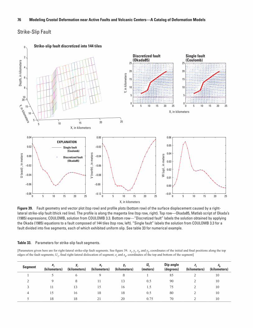
76 Modeling Crustal Deformation near Active Faults and Volcanic Centers—A Catalog of Deformation Models
Figure 39. Fault geometry and vector plot (top row) and profile plots (bottom row) of the surface displacement caused by a right-lateral strike-slip fault (thick red line). The profile is along the magenta line (top row, right). Top row—Okada85, Matlab script of Okada’s (1985) expressions; COULOMB, solution from COULOMB 3.3. Bottom row—“Discretized fault” labels the solution obtained by applying the Okada (1985) equations to a fault composed of 144 tiles (top row, left). “Single fault” labels the solution from COULOMB 3.3 for a fault divided into five segments, each of which exhibited uniform slip. See table 33 for numerical example.
Strike-Slip Fault
Table 33. Parameters for strike-slip fault segments.
[Parameters given here are for right-lateral strike-slip fault segments. See figure 39. xi, yi, xf, and yf, coordinates of the initial and final positions along the top edges of the fault segments; U1, final right-lateral dislocation of segment; zt and zb, coordinates of the top and bottom of the segment]
Segmentxi
(kilometers)yi
(kilometers)xf
(kilometers)yf
(kilometers)U1
(meters)Dip angle(degrees)
zt(kilometers)
zb(kilometers)
1 5 6 9 8 1 85 2 102 9 8 11 13 0.5 90 2 103 11 13 15 16 1.5 75 2 104 15 16 18 18 0.5 80 2 105 18 18 21 20 0.75 70 2 10
men12-7629_fig39
5 10 15 20 255
10
15
20
0
2
4
6
8
10
Strike-slip fault discretized into 144 tiles
X, in kilometers
Y, in kilometers
Dept
h, in
kilo
met
ers
0 5 10 15 20 250
5
10
15
20
25
Discretized fault(Okada85)
Y, in
kilo
met
ers
0 5 10 15 20 250
5
10
15
20
25
Single fault(Coulomb)
X, in kilometers
0 5 10 15 20 25−0.08
−0.06
−0.04
−0.02
0.00
0.02
0.04
U (e
ast)
, in
met
ers
0 5 10 15 20 25−0.12
−0.00
−0.08
−0.06
−0.04
−0.02
0.00
X, in kilometers
V (n
orth
) , in
met
ers
Single fault (Coulomb)
Discretized fault (Okada85)
0 5 10 15 20 25−0.01
0.00
0.01
0.02
0.03
0.04
0.05
0.06
W (u
p) ,
in m
eter
s
EXPLANATION
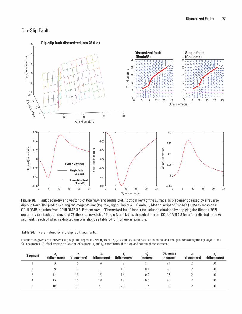
Discretized Faults 77
Figure 40. Fault geometry and vector plot (top row) and profile plots (bottom row) of the surface displacement caused by a reverse dip-slip fault. The profile is along the magenta line (top row, right). Top row—Okada85, Matlab script of Okada’s (1985) expressions; COULOMB, solution from COULOMB 3.3. Bottom row—“Discretized fault” labels the solution obtained by applying the Okada (1985) equations to a fault composed of 78 tiles (top row, left). “Single fault” labels the solution from COULOMB 3.3 for a fault divided into five segments, each of which exhibited uniform slip. See table 34 for numerical example.
men12-7629_fig40
5 10 15 20 255
10
15
20
0
2
4
6
8
10
X, in kilometers
Dept
h, in
kilo
met
ers
0 5 10 15 20 250
5
10
15
20
25
Y, in
kilo
met
ers
0 5 10 15 20 250
5
10
15
20
25
X, in kilometers
0 5 10 15 20 25−0.06
−0.04
−0.02
0
0.02
0.04
0.06
U (e
ast),
in m
eter
s
0 5 10 15 20 25−0.12
−0.1
−0.08
−0.06
−0.04
−0.02
0
X, in kilometers
V (n
orth
), in
met
ers
0 5 10 15 20 25−0.05
0
0.05
0.1
0.15
0.2
W (u
p), i
n m
eter
s
Dip-slip fault discretized into 78 tiles
Discretized fault(Okada85)
Single fault(Coulomb)
Y, in kilometers
Single fault(Coulomb)
Discretized fault(Okada85)
EXPLANATION
Dip-Slip Fault
Table 34. Parameters for dip-slip fault segments.
[Parameters given are for reverse dip-slip fault segments. See figure 40. xi, yi, xf, and yf, coordinates of the initial and final positions along the top edges of the fault segments; U2, final reverse dislocation of segment; zt and zb, coordinates of the top and bottom of the segment.
Segmentxi
(kilometers)yi
(kilometers)xf
(kilometers)yf
(kilometers)U2
(meters)Dip angle (degrees)
zt(kilometers)
zb(kilometers)
1 5 6 9 8 1 85 2 102 9 8 11 13 0.1 90 2 103 11 13 15 16 0.7 75 2 104 15 16 18 18 0.5 80 2 105 18 18 21 20 1.5 70 2 10
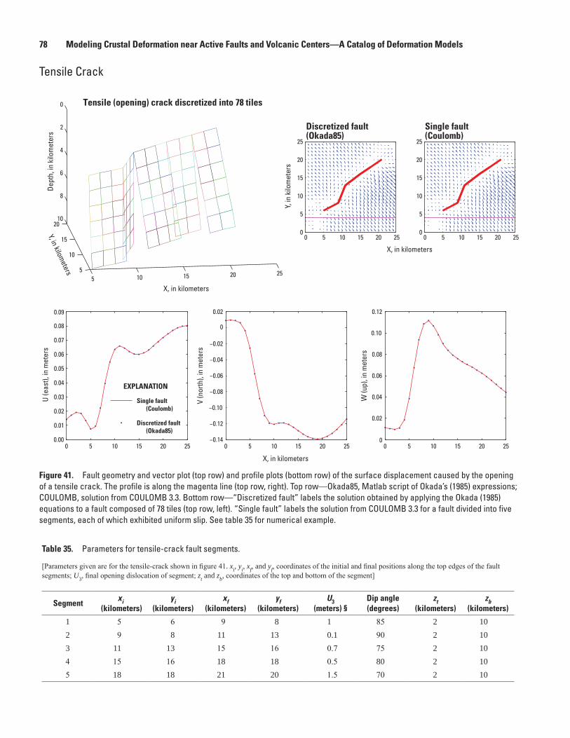
78 Modeling Crustal Deformation near Active Faults and Volcanic Centers—A Catalog of Deformation Models
men12-7629_fig41
5 10 15 20 255
10
15
20
0
2
4
6
8
10
0 5 10 15 20 250
5
10
15
20
25
0 5 10 15 20 250
5
10
15
20
25
Tensile (opening) crack discretized into 78 tiles
X, in kilometers
Y, in kilometers
Dept
h, in
kilo
met
ers
Discretized fault(Okada85)
Y, in
kilo
met
ers
Single fault(Coulomb)
X, in kilometers
0 5 10 15 20 250.00
0.01
0.02
0.03
0.04
0.05
0.06
0.07
0.08
0.09
0 5 10 15 20 25−0.14
−0.12
−0.10
−0.08
−0.06
−0.04
−0.02
0.02
0 5 10 15 20 25
0.02
0.04
0.06
0.08
0.10
0.12
0
0
U (e
ast),
in m
eter
s
X, in kilometers
V (n
orth
), in
met
ers
W (u
p), i
n m
eter
s
Single fault(Coulomb)
Discretized fault(Okada85)
EXPLANATION
Figure 41. Fault geometry and vector plot (top row) and profile plots (bottom row) of the surface displacement caused by the opening of a tensile crack. The profile is along the magenta line (top row, right). Top row—Okada85, Matlab script of Okada’s (1985) expressions; COULOMB, solution from COULOMB 3.3. Bottom row—“Discretized fault” labels the solution obtained by applying the Okada (1985) equations to a fault composed of 78 tiles (top row, left). “Single fault” labels the solution from COULOMB 3.3 for a fault divided into five segments, each of which exhibited uniform slip. See table 35 for numerical example.
Table 35. Parameters for tensile-crack fault segments.
[Parameters given are for the tensile-crack shown in figure 41. xi, yi, xf, and yf, coordinates of the initial and final positions along the top edges of the fault segments; U3, final opening dislocation of segment; zt and zb, coordinates of the top and bottom of the segment]
Segmentxi
(kilometers)yi
(kilometers)xf
(kilometers)yf
(kilometers)U3
(meters) §Dip angle(degrees)
zt(kilometers)
zb(kilometers)
1 5 6 9 8 1 85 2 102 9 8 11 13 0.1 90 2 103 11 13 15 16 0.7 75 2 104 15 16 18 18 0.5 80 2 105 18 18 21 20 1.5 70 2 10
Tensile Crack
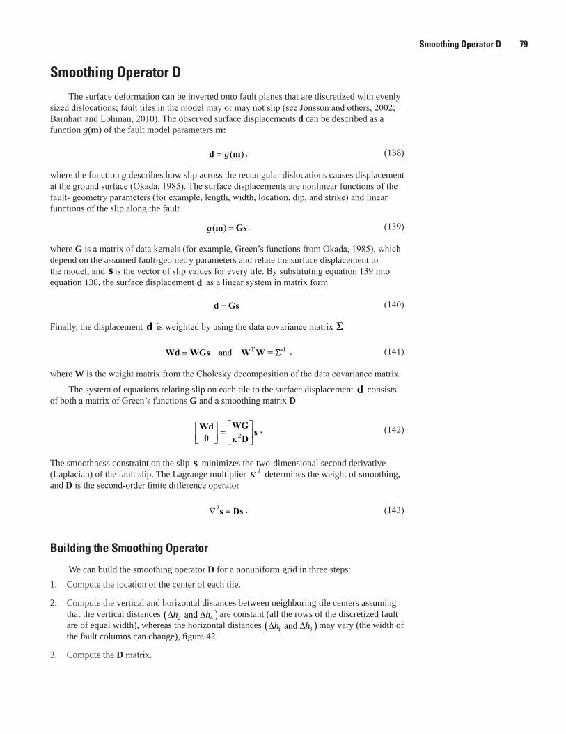
Smoothing Operator D 79
Smoothing Operator DThe surface deformation can be inverted onto fault planes that are discretized with evenly
sized dislocations; fault tiles in the model may or may not slip (see Jonsson and others, 2002; Barnhart and Lohman, 2010). The observed surface displacements d can be described as a function g(m) of the fault model parameters m:
d m= g( ) , (138)
where the function g describes how slip across the rectangular dislocations causes displacement at the ground surface (Okada, 1985). The surface displacements are nonlinear functions of the fault- geometry parameters (for example, length, width, location, dip, and strike) and linear functions of the slip along the fault
g( )m Gs= . (139)
where G is a matrix of data kernels (for example, Green’s functions from Okada, 1985), which depend on the assumed fault-geometry parameters and relate the surface displacement to the model; and s is the vector of slip values for every tile. By substituting equation 139 into equation 138, the surface displacement d as a linear system in matrix form
d Gs= . (140)
Finally, the displacement d is weighted by using the data covariance matrix ΣΣ
Wd WGs W W =T -1= and ΣΣ , (141)
where W is the weight matrix from the Cholesky decomposition of the data covariance matrix.
The system of equations relating slip on each tile to the surface displacement d consists of both a matrix of Green’s functions G and a smoothing matrix D
Wd0
WGDs
=
κ2
, (142)
The smoothness constraint on the slip s minimizes the two-dimensional second derivative (Laplacian) of the fault slip. The Lagrange multiplier κ 2 determines the weight of smoothing, and D is the second-order finite difference operator
∇ =2s Ds . (143)
Building the Smoothing Operator
We can build the smoothing operator D for a nonuniform grid in three steps:1. Compute the location of the center of each tile.
2. Compute the vertical and horizontal distances between neighboring tile centers assuming that the vertical distances ∆ ∆h h2 4 and ( ) are constant (all the rows of the discretized fault are of equal width), whereas the horizontal distances ∆ ∆h h1 3 and ( ) may vary (the width of the fault columns can change), figure 42.
3. Compute the D matrix.
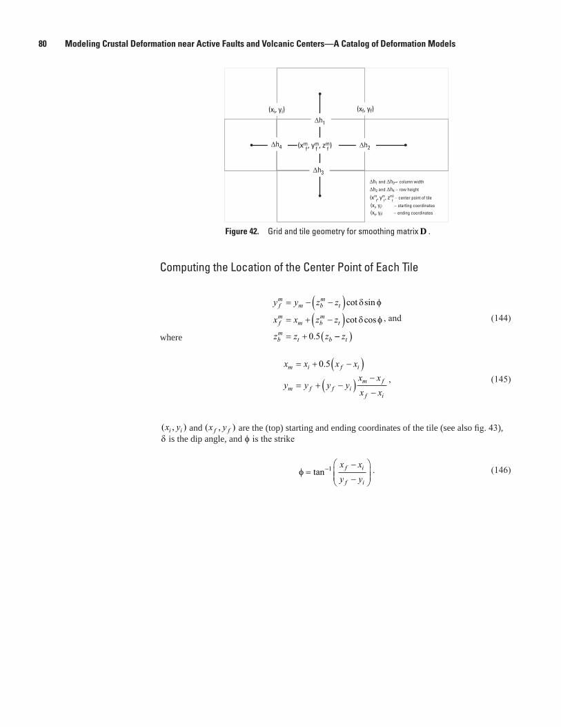
80 Modeling Crustal Deformation near Active Faults and Volcanic Centers—A Catalog of Deformation Models
Computing the Location of the Center Point of Each Tile
y y z z
x x z z
z z z
fm
m bm
t
fm
m bm
t
bm
t b
= − −( )= + −( )= +
cot sin
cot cos
.
δ φ
δ φ
0 5 −−( )zt
, and (144)
where
x x x x
y y y yx xx x
m i f i
m f f im f
f i
= + −( )= + −( ) −
−
0 5.
, (145)
( , )x yi i and ( , )x yf f are the (top) starting and ending coordinates of the tile (see also fig. 43), δ is the dip angle, and φ is the strike
φ =−
−
−tan 1 x xy yf i
f i
. (146)
men12-7629_fig42
(xm, ym, zm)∆h4 ∆h2
∆h1
(xi, yi) (xf, yf)
f f f
∆h3
∆h1 and ∆h3 −̶ column width
∆h2 and ∆h4 − row height
(xm, ym, zm) − center point of tilef f f
(xi, yi) − starting coordinates
(xf, yf) − ending coordinates
Figure 42. Grid and tile geometry for smoothing matrix D .
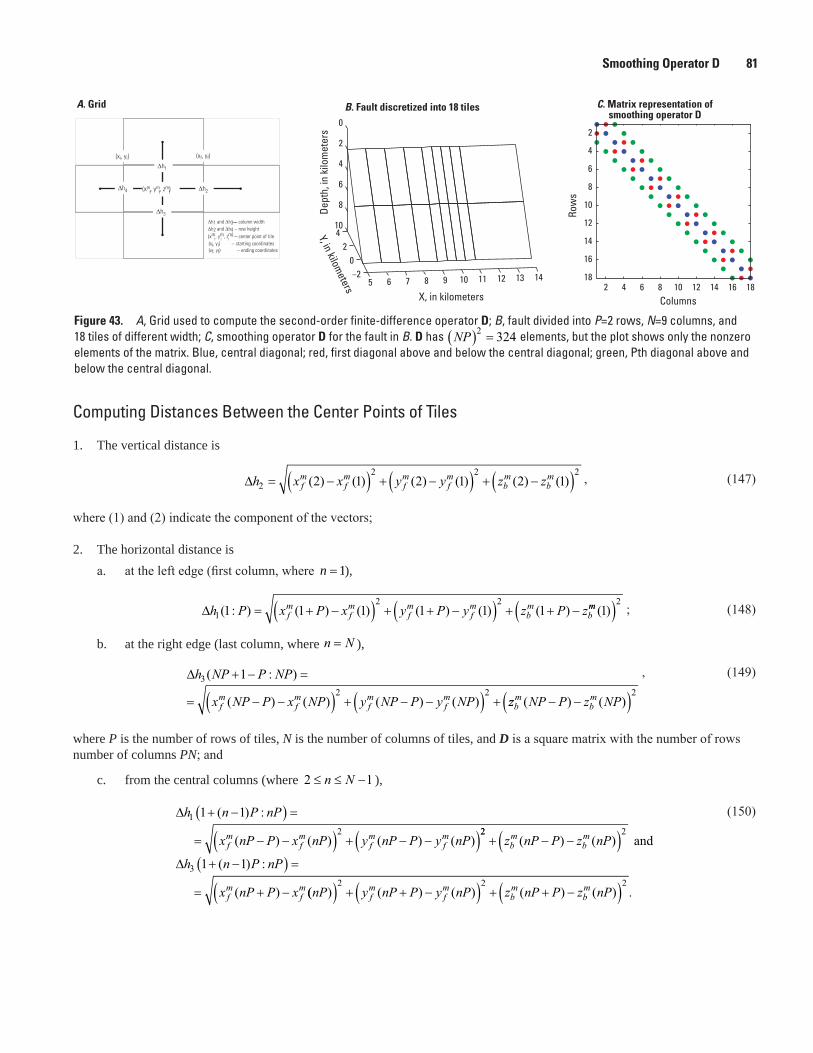
Smoothing Operator D 81
Computing Distances Between the Center Points of Tiles
1. The vertical distance is
∆h x x y y z zfm
fm
fm
fm
bm
bm
22 2 2
2 1 2 1 2 1= −( ) + −( ) + −( )( ) ( ) ( ) ( ) ( ) ( ) , (147)
where (1) and (2) indicate the component of the vectors;
2. The horizontal distance isa. at the left edge (first column, where n = 1),
∆h P x P x y P y z P zfm
fm
fm
fm
bm
b12 2
1 1 1 1 1 1( : ) ( ) ( ) ( ) ( ) ( )= + −( ) + + −( ) + + − mm ( )12( ) ; (148)
b. at the right edge (last column, where n N= ),
∆h NP P NP
x NP P x NP y NP P y NPfm
fm
fm
fm
32 2
1( : )
( ) ( ) ( ) ( )
+ − =
= − −( ) + − −( ) + zz NP P z NPbm
bm( ) ( )− −( )2
, (149)
where P is the number of rows of tiles, N is the number of columns of tiles, and D is a square matrix with the number of rows number of columns PN; and
c. from the central columns (where 2 1≤ ≤ −n N ),
∆h n P nP
x nP P x nP y nP P y nPfm
fm
fm
fm
12
1 1+ −( ) =
= − −( ) + − −( )( ) :
( ) ( ) ( ) ( )22 2
3 1 1
+ − −( )+ −( ) =
= + −
z nP P z nP
h n P nP
x nP P x
bm
bm
fm
fm
( ) ( )
( ) :
( )
and
∆
(( ) ( ) ( ) ( ) ( ) .nP y nP P y nP z nP P z nPfm
fm
bm
bm( ) + + −( ) + + −( )2 2 2
(150)
men12-7629_fig43
C. Matrix representation of smoothing operator D
5 6 7 8 9 10 11 12 13 14−20
24
0
2
4
6
8
10
X, in kilometers
Dept
h, in
kilo
met
ers
B. Fault discretized into 18 tilesA. Grid
2 4 6 8 10 12 14 16 18
2
4
6
8
10
12
14
16
18
(xm, ym, zm)∆h4 ∆h2
∆h1
(xi, yi) (xf, yf)
f f f
∆h3
∆h1 and ∆h3 ̶− column width∆h2 and ∆h4 − row height(xm, ym, zm) − center point of tile
f f f(xi, yi) − starting coordinates (xf, yf) − ending coordinates
Y, in kilometers
Columns
Row
s
Figure 43. A, Grid used to compute the second-order finite-difference operator D; B, fault divided into P=2 rows, N=9 columns, and 18 tiles of different width; C, smoothing operator D for the fault in B. D has NP( ) =2 324 elements, but the plot shows only the nonzero elements of the matrix. Blue, central diagonal; red, first diagonal above and below the central diagonal; green, Pth diagonal above and below the central diagonal.
82 Modeling Crustal Deformation near Active Faults and Volcanic Centers—A Catalog of Deformation Models
Computing the Smoothing Operator DThe smoothing operator D is a second-order finite difference operator (equation 143).
As the slip is determined on discrete tiles (figs. 42 and 43), ∇2s = Ds is a two-dimensional, second-order finite-difference sum
s s s
h h
s s s
hi j i j i j i j i j i j− + − +− +
+( )+
− +1 1
1 32
1 1
22
2 2
4, , , , , ,
∆ ∆ ∆. (151)
The matrix implementing D is always zero, except along a limited number of diagonals (fig. 43C): the central diagonal and the first and Pth diagonals above and below the central diagonal, where P is the number of rows of tiles on the fault (fig. 43B).
Case 1—Fault does not Break the Surface
1. First, compute the central diagonal (0)
dh h h
= − +
2 1 1
1 3 22∆ ∆ ∆
, (152)
2. diagonal (+1)
dph
dp N P dp dp NP122 1 1 1
1 1 0 1 1= ( )( ) = = −∆
, : , ( : ) , (153)
3. diagonal (-1)
dmh
dm N P dm dm NP122 1 1 1
1 1 1 0 2= +( ) = =∆
, ( : ) ( : ) , (154)
4. diagonal (+P)
dp 2h
dp dp 1 NP P4 4 4=+( )
= −( )∆ ∆ ∆h h3 1 3
, : , and finally (155)
5. diagonal (-P)
( ) ( )4 4 4
1 1 3
2 , 1 :dm dm dm P NPh h h
= = +∆ ∆ + ∆
. (156)
Smoothing Operator D 83
Case 2—Fault Breaks the Surface
1. First, compute the central diagonal (0)
( ) ( )( ) ( )( )2 2
1 11 , 1: 1 1 (1) 1: 1 1
d d N Ph h N P
= − + =∆ ∆ − +
, (157)
2. diagonal (+1)
( ) ( )( ) ( )( )1 12 2
1 11 , 1: 1 1(1) 1: 1 1
dp dp N Ph h N P
= − − + = −∆ ∆ − +
, (158)
3. diagonal (-1)
( )( )1 1: 1 0dm N P− = , (159)
4. diagonal (+P) — this condition allows slip in the upper row of tiles to be nonzero when the fault breaks the surface (that is, produces measurable surface offsets)
( ) ( )( )4 41 0, 1: 2 1 0dp dp N P= − + = , and finally (160)
5. diagonal (-P) — see note for step 4.
( ) ( )( )4 41 0, 1: 2 1 0dm dm N P= − + = . (161)
Case 3—Dike Opening at the Base of the Dislocation
1. First, compute the central diagonal (0)
( )( ) ( )( )2
11: 1:
d N Ph N P
=∆
, (162)
2. diagonal (+1)
( )( )1 1: 1 0dp N P− = , (163)
3. diagonal (-1)
( ) ( )( )( ) ( )( )
12
12
11 ,1
11: 1 11: 1 1
dm Ph P
dm N P Ph N P P
− = −∆ −
− + − = −∆ − + −
(164)
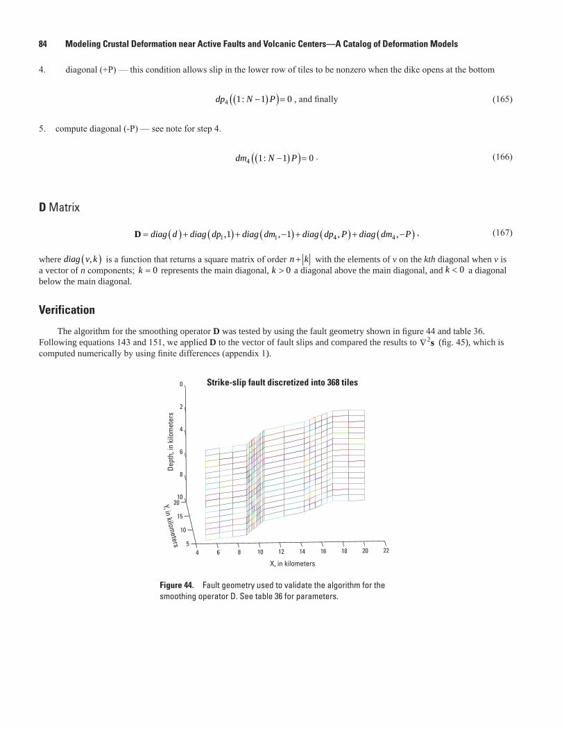
84 Modeling Crustal Deformation near Active Faults and Volcanic Centers—A Catalog of Deformation Models
4. diagonal (+P) — this condition allows slip in the lower row of tiles to be nonzero when the dike opens at the bottom
( )( )4 1: 1 0dp N P− = , and finally (165)
5. compute diagonal (-P) — see note for step 4.
( )( )4 1: 1 0dm N P− = . (166)
D Matrix
( ) ( ) ( ) ( ) ( )1 1 4 4,1 , 1 , ,diag d diag dp diag dm diag dp P diag dm P= + + − + + −D , (167)
where ( ),diag v k is a function that returns a square matrix of order n k+ with the elements of v on the kth diagonal when v is a vector of n components; 0k = represents the main diagonal, 0k > a diagonal above the main diagonal, and 0k < a diagonal below the main diagonal.
Verification
The algorithm for the smoothing operator D was tested by using the fault geometry shown in figure 44 and table 36. Following equations 143 and 151, we applied D to the vector of fault slips and compared the results to 2∇ s (fig. 45), which is computed numerically by using finite differences (appendix 1).
men12-7629_fig44
4 6 8 10 12 14 16 18 20 225
10
15
20
0
2
4
6
8
10
Strike-slip fault discretized into 368 tiles
X, in kilometers
Dept
h, in
kilo
met
ers
Y, in kilometers
Figure 44. Fault geometry used to validate the algorithm for the smoothing operator D. See table 36 for parameters.
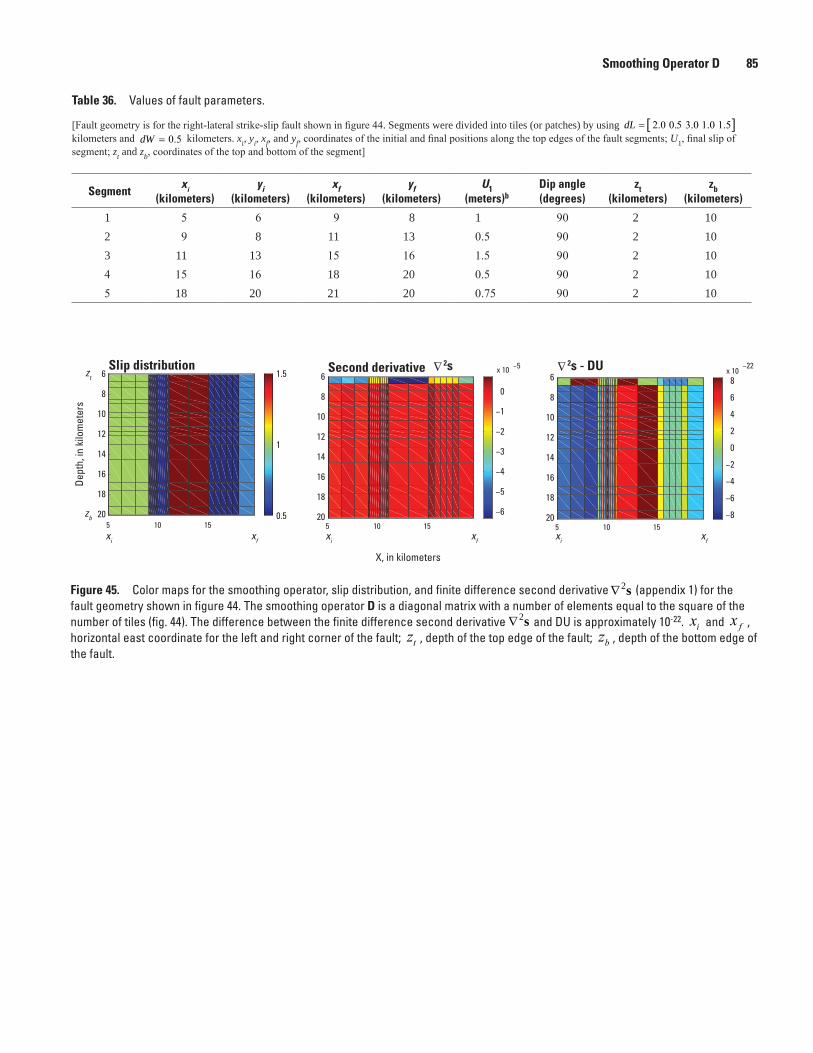
Smoothing Operator D 85
Table 36. Values of fault parameters.
[Fault geometry is for the right-lateral strike-slip fault shown in figure 44. Segments were divided into tiles (or patches) by using [ ]2.0 0.5 3.0 1.0 1.5dL = kilometers and 0.5dW = kilometers. xi, yi, xf, and yf, coordinates of the initial and final positions along the top edges of the fault segments; U1, final slip of segment; zt and zb, coordinates of the top and bottom of the segment]
Segmentxi
(kilometers) yi
(kilometers)xf
(kilometers)yf
(kilometers)U1
(meters)bDip angle(degrees)
zt(kilometers)
zb(kilometers)
1 5 6 9 8 1 90 2 102 9 8 11 13 0.5 90 2 103 11 13 15 16 1.5 90 2 104 15 16 18 20 0.5 90 2 105 18 20 21 20 0.75 90 2 10
men12-7629_fig45
−5
5 10 15
6
8
10
12
14
16
18
20
Slip distribution
0.5
1
1.5
Dept
h, in
kilo
met
ers
zt
zb
xi xf
X, in kilometers
xi xf xi xf
5 10 15
6
8
10
12
14
16
18
20 −6
−5
−4
−3
−2
−1
0
x 10Second derivative
5 10 15−8
−6
−4
−2
0
2
4
6
8x 10
−226
8
10
12
14
16
18
20
∆2s - DU∆2s
Figure 45. Color maps for the smoothing operator, slip distribution, and finite difference second derivative 2∇ s (appendix 1) for the fault geometry shown in figure 44. The smoothing operator D is a diagonal matrix with a number of elements equal to the square of the number of tiles (fig. 44). The difference between the finite difference second derivative 2∇ s and DU is approximately 10-22. xi and x f , horizontal east coordinate for the left and right corner of the fault; zt , depth of the top edge of the fault; zb , depth of the bottom edge of the fault.
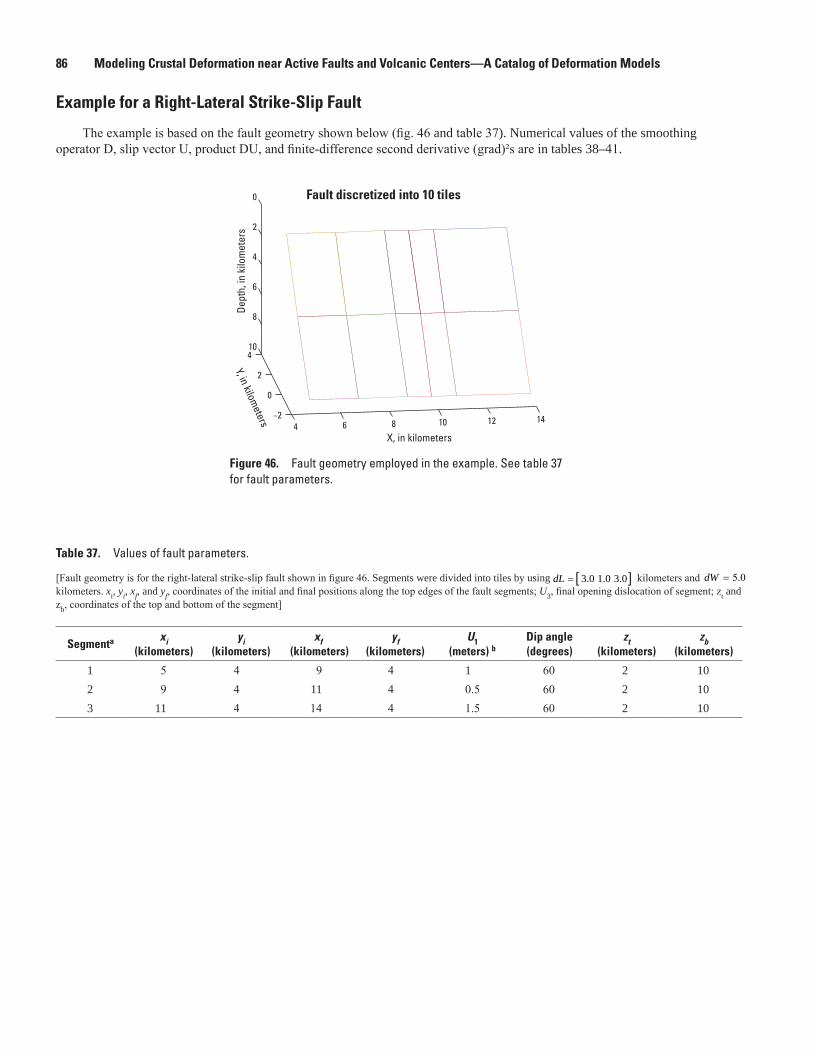
86 Modeling Crustal Deformation near Active Faults and Volcanic Centers—A Catalog of Deformation Models
Example for a Right-Lateral Strike-Slip Fault
The example is based on the fault geometry shown below (fig. 46 and table 37). Numerical values of the smoothing operator D, slip vector U, product DU, and finite-difference second derivative (grad)²s are in tables 38–41.
Figure 46. Fault geometry employed in the example. See table 37 for fault parameters.
men12-7629_fig46
4 6 8 10 12 14−2
0
2
4
0
2
4
6
8
10
Fault discretized into 10 tiles
X, in kilometers
Dept
h, in
kilo
met
ers
Y, in kilometers
Table 37. Values of fault parameters.
[Fault geometry is for the right-lateral strike-slip fault shown in figure 46. Segments were divided into tiles by using [ ]3.0 1.0 3.0dL = kilometers and 5.0dW = kilometers. xi, yi, xf, and yf, coordinates of the initial and final positions along the top edges of the fault segments; U3, final opening dislocation of segment; zt and zb, coordinates of the top and bottom of the segment]
Segmenta xi (kilometers)
yi(kilometers)
xf (kilometers)
yf(kilometers)
U1(meters) b
Dip angle(degrees)
zt(kilometers)
zb(kilometers)
1 5 4 9 4 1 60 2 102 9 4 11 4 0.5 60 2 103 11 4 14 4 1.5 60 2 10
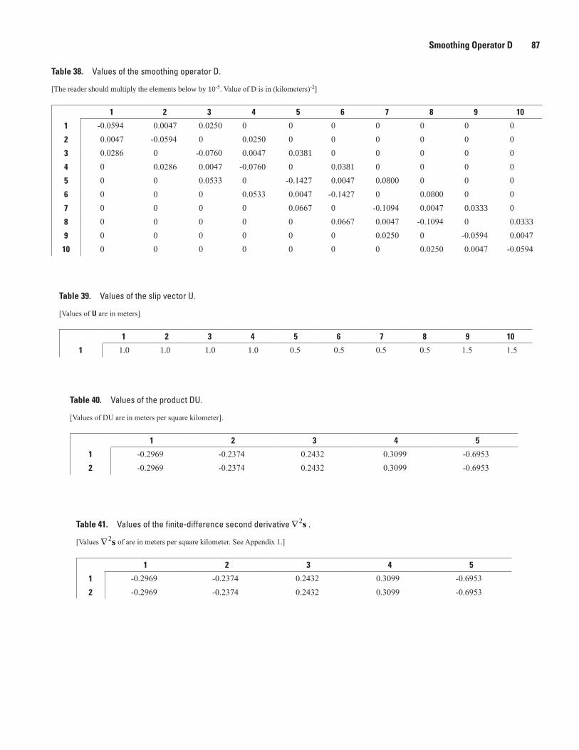
Smoothing Operator D 87
Table 38. Values of the smoothing operator D.
[The reader should multiply the elements below by 10-5. Value of D is in (kilometers)-2]
1 2 3 4 5 6 7 8 9 10
1 -0.0594 0.0047 0.0250 0 0 0 0 0 0 02 0.0047 -0.0594 0 0.0250 0 0 0 0 0 03 0.0286 0 -0.0760 0.0047 0.0381 0 0 0 0 04 0 0.0286 0.0047 -0.0760 0 0.0381 0 0 0 05 0 0 0.0533 0 -0.1427 0.0047 0.0800 0 0 06 0 0 0 0.0533 0.0047 -0.1427 0 0.0800 0 07 0 0 0 0 0.0667 0 -0.1094 0.0047 0.0333 08 0 0 0 0 0 0.0667 0.0047 -0.1094 0 0.03339 0 0 0 0 0 0 0.0250 0 -0.0594 0.0047
10 0 0 0 0 0 0 0 0.0250 0.0047 -0.0594
Table 39. Values of the slip vector U.
[Values of U are in meters]
1 2 3 4 5 6 7 8 9 10
1 1.0 1.0 1.0 1.0 0.5 0.5 0.5 0.5 1.5 1.5
Table 40. Values of the product DU.
[Values of DU are in meters per square kilometer].
1 2 3 4 5
1 -0.2969 -0.2374 0.2432 0.3099 -0.69532 -0.2969 -0.2374 0.2432 0.3099 -0.6953
Table 41. Values of the finite-difference second derivative 2∇ s .
[Values 2∇ s of are in meters per square kilometer. See Appendix 1.]
1 2 3 4 5
1 -0.2969 -0.2374 0.2432 0.3099 -0.69532 -0.2969 -0.2374 0.2432 0.3099 -0.6953
88 Modeling Crustal Deformation near Active Faults and Volcanic Centers—A Catalog of Deformation Models
SummaryThis report is a practical reference for readers interested in applying mathematical models
to investigate volcano and earthquake physics. The report emphasizes the application of analytical models to fit and interpret ground deformation. Although analytical models are based on numerous simplifications (for example, the assumption that the crust is a homogenous, isotropic, elastic, flat half-space) that make the set of differential equations describing the problem tractable, they can take into account a vast array of source geometries. The careful use of analytical models, together with high-quality data sets, can yield valuable insights into the nature of the deformation source.
The paper introduces analytical formulation that describe the deformation caused by magma chambers, magma conduit, sill, dikes and faults, and provides tables with numerical examples and Matlab scripts to aid in the use and coding of the formulas. All formulas have been checked for errors and verified against numerical models (COULOMB 3.3; http://earthquake.usgs.gov/research/modeling/coulomb/; FEM models). A zipped file with MATLAB scripts can be downloaded from http://pubs.usgs.gov/tm/13/b1.
Suggestions about new models that could be included in future revisions, reports of existing bugs in the Matlab scripts (or errors in the formulas) and comments on how to improve this publication will be greatly appreciated.
References Cited
Amoruso, Antonella, and Crescentini, Luca, 2009, Shape and volume change of pressurized ellipsoidal cavities from deformation and seismic data: Journal of Geophysical Research, v. 114, B02210 (also available at http://dx.doi.org/ 10.1029/2008JB005946).
Barnhart, W.D., and Lohman, R.B., 2010, Automated fault model discretization for inversions for coseismic slip distributions: Journal of Geophysical Research, v. 115, B10419, 17 p. (also available at http://dx.doi.org/ 10.1029/2010JB007545).
Cervelli, P.F., Fournier, T.J., Freymueller, J.T., and Power, J.A., 2006, Ground deformation associated with the precursory unrest and early phases of the January 2006 eruption of Augustine Volcano, Alaska: Geophysical Research Letters, v. 33, L18304 (also available at http://dx.doi.org/ 10.1029/2006GL027219).
Dawson, John, and Woods, Alex, 2010, ITRF to GDA94 Coordinate Transformations: Journal of Applied Geodesy, v. 4, 189–199 (also available at http://dx.doi.org/ 10.1515/JAG.2010.019)
Defense Mapping Agency (DMA), 1989, The Universal Grids—Universal Transverse Mercator (UTM) and Universal Polar Stereographic (UPS): Fairfax, Va., DMA Technical Manual DMATM 8358.2.
Dzurisin, Daniel, 2003, A comprehensive approach to monitoring volcano deformation as a window on the eruption cycle: Review of Geophysics, v. 41, no. 1, 1001 p. (also available at http://dx.doi.org/10.1029/2001RG000107).
Fialko, Y., Khazan, Y., and Simons, M., 2001, Deformation due to a pressurized horizontal circular crack in an elastic half-space, with applications to volcano geodesy: Geophysical Journal International, v. 146, no.1, p. 181–190.
Hoffmann-Wellenhof, B., Lichtenegger, H., and Collins, J., 1997, Global positioning system—Theory and practice (4th revised ed.): New York and Vienna, Springer, 389 p.

References Cited 89
Jónsson, S., Zebker, H., Segall, P., and Amelung, F., 2002, Fault slip distribution of the 1999 M7.2 Hector Mine earthquake, California, estimated from satellite radar and GPS measurements: Bulletin of the Seismological Society of America, v. 92, no. 4, p. 1377–1389.
Masterlark, Timothy, 2007, Magma instrusion and deformation predictions—Sensitivities to the Mogi assumptions: Journal of Geophysical Research, v. 112, no. B06419, 17 p. (also available at http://dx.doi.org/10.1029/2006JB004860).
McTigue, D.F., 1987, Elastic stress and deformation near a finite spherical magma body—Resolution of the point source paradox: Journal of Geophysical Research, v. 92, no. B12, p. 12931–12940 (also available at http://dx.doi.org/10.1029/JB092iB12p12931).
National Imagery and Mapping Agency (NIMA), 2000, Department of Defense World Geodetic System 1984—Its definition and relationship with local geodetic systems: Technical Report TR8350.2.
National Imagery and Mapping Agency (NIMA), 2004, Implementation of the World Geodetic System 1984 (WGS 84) Reference Frame G1150. Addendum to NIMA TR 8350.2.
Newman, A.V., Dixon, T.H., and Gourmelen, N., 2006, A four-dimensional viscoelastic deformation model for Long Valley Caldera, California, between 1995 and 2000: Journal of Volcanology and Geothermal Research, v. 150, p. 244–269.
Okada, Yoshimitsu, 1985, Surface deformation due to shear and tensile faults in a half-space: Bulletin of the Seismological Society of America, v. 75, no. 4, p. 1135–1154.
Okada, Yoshimitsu, 1992, Internal deformation due to shear and tensile faults in a half-space: Bulletin of the Seismological Society of America, v. 82, no. 2, p. 1018–1040.
Press, W.H., Teukolsky, S.A., Vetterling, W.T., and Flannery, B.P., 1992, Numerical recipes in Fortran 77—The Art of Scientific Computing (2d ed.), v. 1: Cambridge, Cambridge University Press, 921 p.
Segall, Paul, 2010, Earthquake and volcano deformation: Princeton, N.J., Princeton University Press, 458 p.
Tiampo, K.F., Rundle, J.B., Fernandez, J., and Langbein, J.O., 2000, Spherical and ellipsoidal volcanic sources at Long Valley caldera, California, using a genetic algorithm inversion technique: Journal of Volcanology and Geothermal Research, v. 102, no. 3, p. 189–206.
U.S. Army, 1987, Standard UTM-to-GEO/GEO-to-UTM Coordinate Conversion Algorithm: Technical Manual TM 5–241–8 (accessed on August 2, 2012 at http://ntrs.nasa.gov/archive/nasa/casi.ntrs.nasa.gov/19890002875_1989002875.pdf).
Yang, X.-M., Davis, P.M., and Dieterich, J.H., 1988, Deformation from inflation of a dipping finite prolate spheroid in an elastic half-space as a model for volcanic stressing: Journal of Geophysical Research, v. 93, no. B5, p. 4249–4257.
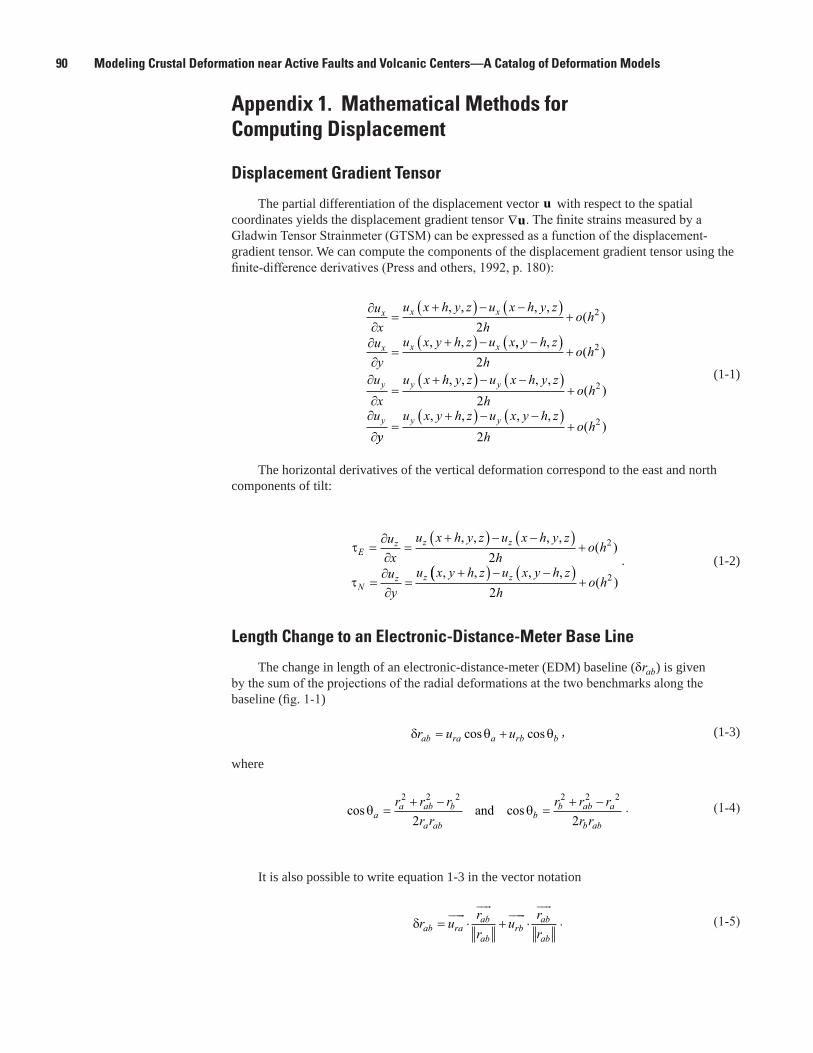
90 Modeling Crustal Deformation near Active Faults and Volcanic Centers—A Catalog of Deformation Models
Appendix 1. Mathematical Methods for Computing Displacement
Displacement Gradient Tensor
The partial differentiation of the displacement vector u with respect to the spatial coordinates yields the displacement gradient tensor ∇u. The finite strains measured by a Gladwin Tensor Strainmeter (GTSM) can be expressed as a function of the displacement-gradient tensor. We can compute the components of the displacement gradient tensor using the finite-difference derivatives (Press and others, 1992, p. 180):
∂∂
=+( ) − −( )
+
∂∂
=+( ) −
ux
u x h y z u x h y zh
o h
uy
u x y h z u x
x x x
x x x
, , , ,( )
, ,2
2
,, ,( )
, , , ,( )
y h zh
o h
ux
u x h y z u x h y zh
o h
u
y y y
y
−( )+
∂
∂=
+( ) − −( )+
∂
∂
2
2
2
2
yyu x y h z u x y h z
ho hy y=
+( ) − −( )+
, , , ,( )
22
(1-1)
The horizontal derivatives of the vertical deformation correspond to the east and north components of tilt:
τ
τ
Ez z z
Nz z
ux
u x h y z u x h y zh
o h
uy
u x y h z
=∂∂
=+( ) − −( )
+
=∂∂
=+
, , , ,( )
, ,2
2
(( ) − −( )+
u x y h zh
o hz , ,( )
22
. (1-2)
Length Change to an Electronic-Distance-Meter Base Line
The change in length of an electronic-distance-meter (EDM) baseline (δrab) is given by the sum of the projections of the radial deformations at the two benchmarks along the baseline (fig. 1-1)
δ θ θr u uab ra a rb b= +cos cos , (1-3)
where
cos cosθ θaa ab b
a abb
b ab a
b ab
r r rr r
r r rr r
=+ −
=+ −2 2 2 2 2 2
2 2and . (1-4)
It is also possible to write equation 1-3 in the vector notation
δr urr
urrab ra
ab
abrb
ab
ab= ⋅ + ⋅� ��� � �� � ��� � ��
. (1-5)
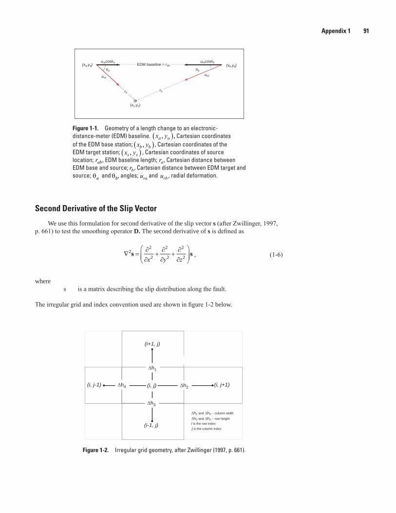
Appendix 1 91
Second Derivative of the Slip Vector
We use this formulation for second derivative of the slip vector s (after Zwillinger, 1997, p. 661) to test the smoothing operator D. The second derivative of s is defined as
∇ =∂∂
+∂∂
+∂∂
22
2
2
2
2
2s sx y z
, (1-6)
where s is a matrix describing the slip distribution along the fault.
The irregular grid and index convention used are shown in figure 1-2 below.
Figure 1-1. Geometry of a length change to an electronic-distance-meter (EDM) baseline. x ya a,( ) , Cartesian coordinatesof the EDM base station; x yb b,( ) , Cartesian coordinates of theEDM target station; x ys s,( ) , Cartesian coordinates of sourcelocation; rab, EDM baseline length; ra, Cartesian distance between EDM base and source; rb , Cartesian distance between EDM target and source; θa and θb, angles; ura and urb , radial deformation.
(xa,ya)uracosθa
(xs,ys)
(xb,yb)
uraurb
ra
θa θb
urbcosθb
rb
EDM baseline = rab
(i, j)∆h4 ∆h2
∆h1
∆h3
∆h1 and ∆h3 − column width
∆h2 and ∆h4 − row height
(i+1, j)
(i-1, j)
(i, j-1) (i, j+1)
i is the row indexj is the column index
Figure 1-2. Irregular grid geometry, after Zwillinger (1997, p. 661).
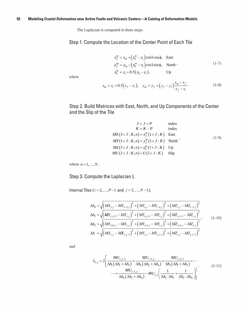
92 Modeling Crustal Deformation near Active Faults and Volcanic Centers—A Catalog of Deformation Models
The Laplacian is computed in three steps:
Step 1. Compute the Location of the Center Point of Each Tile
( )( )
( )
cot cos , East
cot sin , North
0.5 , Up
m mf m b t
m mf m b tmb t b t
x x z z
y y z z
z z z z
= + − δ φ
= − − δ φ
= + −
, (1-7)
where
x x x x y y y yx xx xm i f i m f f im f
f i= + −( ) = + −( ) −
−0 5. , . (1-8)
Step 2. Build Matrices with East, North, and Up Components of the Center and the Slip of the Tile
( ) ( )( ) ( )( ) ( )( ) ( )
index– index
1 : , 1 : East
1 : , 1 : North
1 : , 1 : Up1 : , 1 : Slip
mfmfmb
J J PK K P
MX J K n x J KMY J K n y J KMZ J K n z J KMU J K n U J K
= +=
+ = +
+ = +
+ = ++ = +
, (1-9)
where n N= 1, , .
Step 3. Compute the Laplacian L
Internal Tiles ( i P= −2 1, , and j N= −2 1, , ),
∆
∆
h MX MX MY MY MZ MZ
h
i j i j i j i j i j i j4 12
12
12
3
= −( ) + −( ) + −( )=
− − −, , , , , ,
MMX MX MY MY MZ MZ
h MX
i j i j i j i j i j i j
i
, , , , , ,+ + +−( ) + −( ) + −( )=
12
12
12
2∆ ++ + +−( ) + −( ) + −( )= −
12
12
12
, , , , , ,
,
j i j i j i j i j i j
i j
MX MY MY MZ MZ
h MX M∆ XX MY MY MZ MZi j i j i j i j i j, , , , ,− − −( ) + −( ) + −( )12
12
12
, (1-10)
and
( ) ( ) ( )
( )
, 1 1, , 1,
1 1 3 2 2 4 3 1 3
1,,
4 2 4 1 3 2 4
2
1 1
i j i j i ji j
i ji j
MU MU MUL
h h h h h h h h hMU
MUh h h h h h h
− + +
−
= + + +
∆ ∆ + ∆ ∆ ∆ + ∆ ∆ ∆ + ∆
+ − + ∆ ∆ + ∆ ∆ ⋅ ∆ ∆ ⋅ ∆
. (1-11)
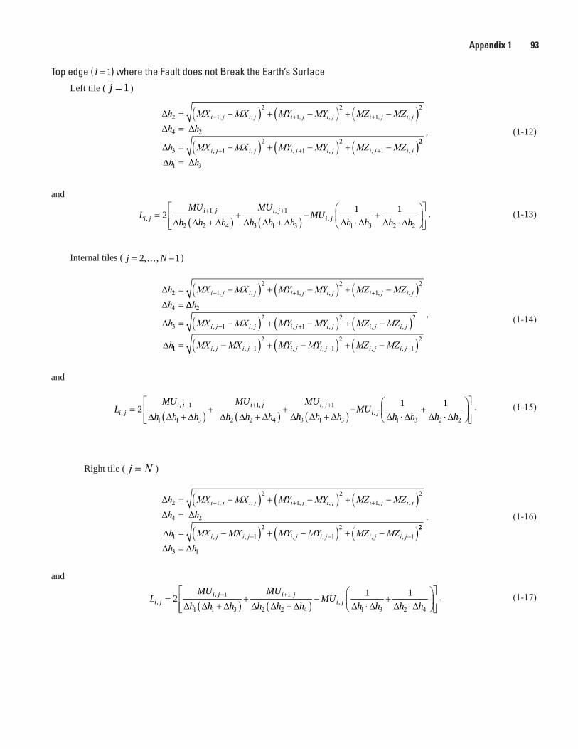
Appendix 1 93
Top edge ( i = 1) where the Fault does not Break the Earth’s SurfaceLeft tile ( j =1)
∆
∆
h MX MX MY MY MZ MZh
i j i j i j i j i j i j2 12
12
12
4
= −( ) + −( ) + −( )=
+ + +, , , , , ,
∆
∆
h
h MX MX MY MY MZ MZi j i j i j i j i j i j
2
3 12
12
1= −( ) + −( ) + −( )+ + +, , , , , ,22
1 3∆ ∆h h=
, (1-12)
and
( ) ( )
1, , 1, ,
2 2 4 3 1 3 1 3 2 2
1 1 2 i j i ji j i j
MU MUL MU
h h h h h h h h h h+ +
= + − + ∆ ∆ + ∆ ∆ ∆ + ∆ ∆ ⋅ ∆ ∆ ⋅ ∆ . (1-13)
Internal tiles ( 2, , 1j N= −)
∆
∆
h MX MX MY MY MZ MZh
i j i j i j i j i j i j2 12
12
12
4
= −( ) + −( ) + −( )=
+ + +, , , , , ,
∆∆
∆
∆
h
h MX MX MY MY MZ MZ
h
i j i j i j i j i j i j
2
3 12
12 2
= −( ) + −( ) + −( )+ +, , , , , ,
11 12
12
12
= −( ) + −( ) + −( )− − −MX MX MY MY MZ MZi j i j i j i j i j i j, , , , , ,
’ (1-14)
and
( ) ( ) ( )
, 1 1, , 1, ,
1 1 3 2 2 4 3 1 3 1 3 2 2
1 1 2 i j i j i ji j i j
MU MU MUL MU
h h h h h h h h h h h h h− + +
= + + − + ∆ ∆ + ∆ ∆ ∆ + ∆ ∆ ∆ + ∆ ∆ ⋅ ∆ ∆ ⋅ ∆ . (1-15)
Right tile ( j N= )
∆
∆
h MX MX MY MY MZ MZh
i j i j i j i j i j i j2 12
12
12
4
= −( ) + −( ) + −( )=
+ + +, , , , , ,
∆
∆
h
h MX MX MY MY MZ MZi j i j i j i j i j i j
2
1 12
12
1= −( ) + −( ) + −( )− − −, , , , , ,22
3 1∆ ∆h h=
, (1-16)
and
( ) ( )
, 1 1,, ,
1 1 3 2 2 4 1 3 2 4
1 1 2 i j i ji j i j
MU MUL MU
h h h h h h h h h h− +
= + − + ∆ ∆ + ∆ ∆ ∆ + ∆ ∆ ⋅ ∆ ∆ ⋅ ∆ . (1-17)
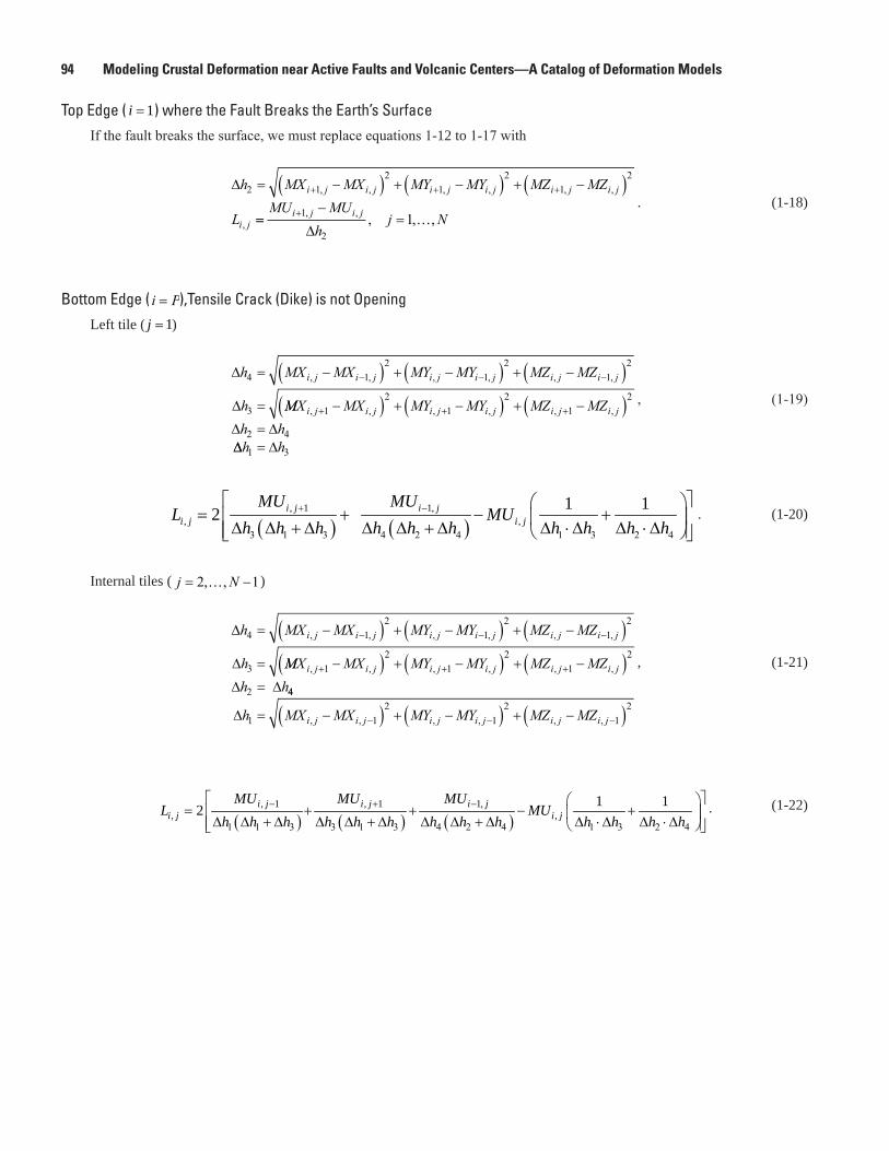
94 Modeling Crustal Deformation near Active Faults and Volcanic Centers—A Catalog of Deformation Models
Top Edge ( i = 1) where the Fault Breaks the Earth’s SurfaceIf the fault breaks the surface, we must replace equations 1-12 to 1-17 with
∆h MX MX MY MY MZ MZ
L
i j i j i j i j i j i j
i j
2 12
12
12
= −( ) + −( ) + −( )+ + +, , , , , ,
, ==−
=+MU MUj N
hi j i j1
21, , , , ,
∆
. (1-18)
Bottom Edge ( i P= ),Tensile Crack (Dike) is not OpeningLeft tile ( j = 1)
∆
∆
h MX MX MY MY MZ MZ
h
i j i j i j i j i j i j4 12
12
12
3
= −( ) + −( ) + −( )=
− − −, , , , , ,
MMX MX MY MY MZ MZh h
i j i j i j i j i j i j, , , , , ,+ + +−( ) + −( ) + −( )=
12
12
12
2 4∆ ∆∆∆ ∆h h1 3=
, (1-19)
( ) ( )
, 1 1,, ,
3 1 3 4 2 4 1 3 2 4
1 12 i j i ji j i j
MU MUL MU
h h h h h h h h h h+ −
= + − + ∆ ∆ + ∆ ∆ ∆ + ∆ ∆ ⋅∆ ∆ ⋅∆ . (1-20)
Internal tiles ( j N= −2 1, ,)
∆
∆
h MX MX MY MY MZ MZ
h
i j i j i j i j i j i j4 12
12
12
3
= −( ) + −( ) + −( )=
− − −, , , , , ,
MMX MX MY MY MZ MZh h
i j i j i j i j i j i j, , , , , ,+ + +−( ) + −( ) + −( )=
12
12
12
2∆ ∆ 44
1 12
12
12
∆h MX MX MY MY MZ MZi j i j i j i j i j i j= −( ) + −( ) + −( )− − −, , , , , ,
, (1-21)
( ) ( ) ( )
, 1 , 1 1,, ,
1 1 3 3 1 3 4 2 4 1 3 2 4
1 12 i j i j i ji j i j
MU MU MUL MU
h h h h h h h h h h h h h− + −
= + + − + ∆ ∆ + ∆ ∆ ∆ + ∆ ∆ ∆ + ∆ ∆ ⋅ ∆ ∆ ⋅ ∆ . (1-22)
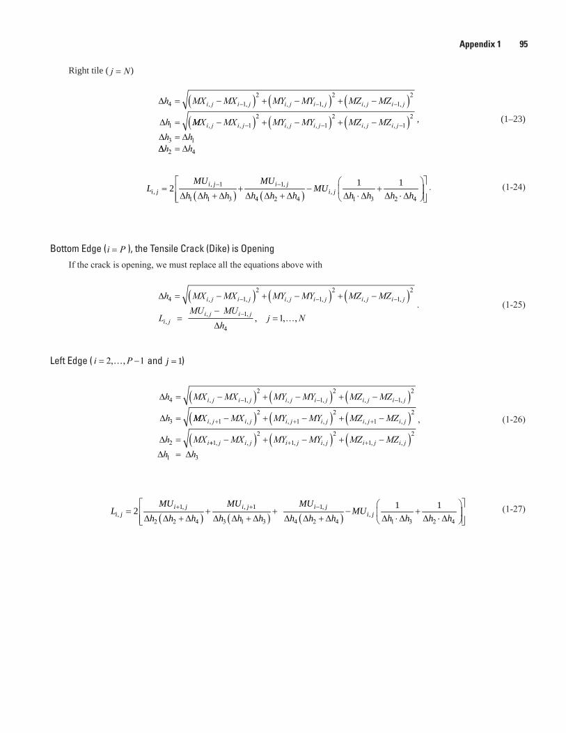
Appendix 1 95
Right tile ( j N= )
∆
∆
h MX MX MY MY MZ MZ
h
i j i j i j i j i j i j4 12
12
12
1
= −( ) + −( ) + −( )=
− − −, , , , , ,
MMX MX MY MY MZ MZh h
i j i j i j i j i j i j, , , , , ,−( ) + −( ) + −( )=
− − −12
12
12
3 1∆ ∆∆∆ ∆h h2 4=
, (1–23)
( ) ( )
, 1 1,, ,
1 1 3 4 2 4 1 3 2 4
1 12 i j i ji j i j
MU MUL MU
h h h h h h h h h h− −
= + − + ∆ ∆ + ∆ ∆ ∆ + ∆ ∆ ⋅ ∆ ∆ ⋅ ∆ . (1-24)
Bottom Edge (i P= ), the Tensile Crack (Dike) is OpeningIf the crack is opening, we must replace all the equations above with
∆h MX MX MY MY MZ MZ
L
i j i j i j i j i j i j
i j
4 12
12
12
= −( ) + −( ) + −( )− − −, , , , , ,
,
=−
= …−MU MUj N
hi j i j, , , , ,1
41
∆
. (1-25)
Left Edge ( i P= −2 1, , and j = 1)
∆
∆
h MX MX MY MY MZ MZ
h
i j i j i j i j i j i j4 12
12
12
3
= −( ) + −( ) + −( )=
− − −, , , , , ,
MMX MX MY MY MZ MZ
h MX
i j i j i j i j i j i j
i
, , , , , ,+ + +−( ) + −( ) + −( )=
12
12
12
2∆ ++ + +−( ) + −( ) + −( )=
12
12
12
1 3
, , , , , ,j i j i j i j i j i jMX MY MY MZ MZh h∆ ∆
, (1-26)
( ) ( ) ( )
1, , 1 1,, ,
2 2 4 3 1 3 4 2 4 1 3 2 4
1 12 i j i j i ji j i j
MU MU MUL MU
h h h h h h h h h h h h h+ + −
= + + − + ∆ ∆ + ∆ ∆ ∆ + ∆ ∆ ∆ + ∆ ∆ ⋅ ∆ ∆ ⋅ ∆ (1-27)
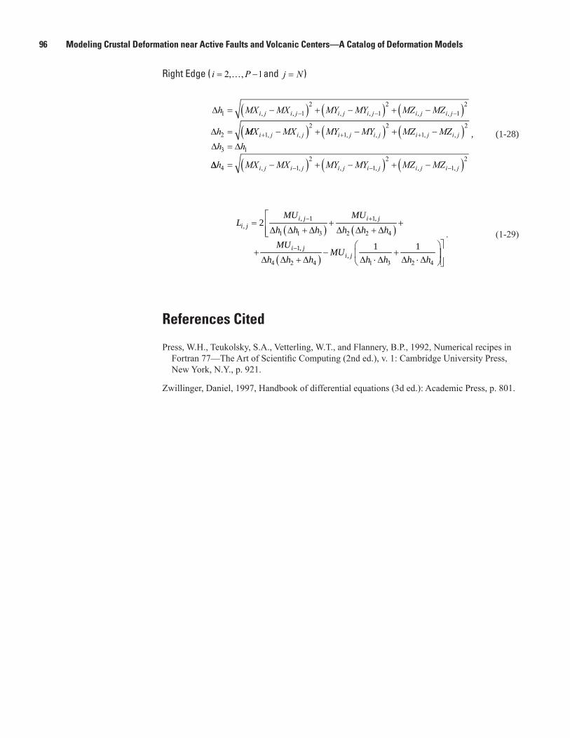
96 Modeling Crustal Deformation near Active Faults and Volcanic Centers—A Catalog of Deformation Models
Right Edge ( i P= −2 1, , and j N= )
∆
∆
h MX MX MY MY MZ MZ
h
i j i j i j i j i j i j1 12
12
12
2
= −( ) + −( ) + −( )=
− − −, , , , , ,
MMX MX MY MY MZ MZh h
i j i j i j i j i j i j+ + +−( ) + −( ) + −( )=
12
12
12
3 1
, , , , , ,
∆ ∆
∆∆h MX MX MY MY MZ MZi j i j i j i j i j i j4 12
12
12
= −( ) + −( ) + −( )− − −, , , , , ,
, (1-28)
( ) ( )
( )
, 1 1,,
1 1 3 2 2 4
1,,
4 2 4 1 3 2 4
2
1 1
i j i ji j
i ji j
MU MUL
h h h h h hMU
MUh h h h h h h
− +
−
= + +
∆ ∆ + ∆ ∆ ∆ + ∆
+ − + ∆ ∆ + ∆ ∆ ⋅ ∆ ∆ ⋅ ∆
. (1-29)
References Cited
Press, W.H., Teukolsky, S.A., Vetterling, W.T., and Flannery, B.P., 1992, Numerical recipes in Fortran 77—The Art of Scientific Computing (2nd ed.), v. 1: Cambridge University Press, New York, N.Y., p. 921.
Zwillinger, Daniel, 1997, Handbook of differential equations (3d ed.): Academic Press, p. 801.

Publishing support provided by the U.S. Geological SurveyPublishing Network, Tacoma Publishing Service Center
For additional information contact:Director, Menlo Park Science CenterU.S. Geological Survey345 Middlefield Road MS 977Menlo Park, California 94025http://earthquake.usgs.gov/regional/nca/

Battaglia and others— M
odeling Crustal Deform
ation near Active Faults and Volcanic Centers—
A Catalog of D
eformation M
odels—TM
13-B1