Gunther Schauberger & Andreas Groll & Gerhard Tutz

Modeling Football Results in the German BundesligaUsing Match-specific Covariates

Technical Report Number 197, 2016Department of StatisticsUniversity of Munich

http://www.stat.uni-muenchen.de

Modeling Football Results in the GermanBundesliga Using Match-specific Covariates

Gunther Schauberger, Andreas Groll & Gerhard TutzDepartment of Statistics, LMU Munich

August 3, 2016

Abstract

In modern football, various variables as, for example, the distances theteams run or the percentages of ball possession, are collected throughout amatch. However, there is a lack of methods to make use of these variablessimultaneously and to connect them with the final result of the match. Thispaper considers data from the German Bundesliga season 2015/16. Theobjective is to identify the variables that are connected to the sportivesuccess or failure of the single teams. A paired comparison model forfootball matches is proposed that is able to take into account match-specificcovariates. The model extends the Bradley-Terry model in many differentways. In addition to the inclusion of covariates, it uses ordered responsevalues and includes (possibly team-specific) home effects. Penalty termsare used to reduce the complexity of the model and to find clusters ofteams with equal covariate effects.

Keywords: Paired Comparison, Bradley-Terry, penalization, BTLLasso.

1 Introduction

Traditionally, discussions about football (and football tactics in particular) arevery controversial, both amongst professional and (us) non-professional footballexperts. After all, most football enthusiasts generally agree on platitudes like theimportance of winning tackles or running more than the opponent. This workaims at contributing to these discussions from a scientific point of view and tothe examination of the validity of football platitudes. In modern football, severalmatch-specific variables as, for example, the running performance of teams or thetackling rate are measured and are publicly available from several online media.We will consider a specific regression model incorporating a set of covariates ofthat kind.

1

From a statistical point of view, a football match between two competingteams can be seen as a paired comparison. In paired comparisons, two objects arecompared and it is observed, which of the objects dominates. It is assumed, thatthe dominance is generated by an unobserved latent trait. In football matches,the latent traits are the playing abilities of both teams. The standard modelfor paired comparisons is the Bradley-Terry model (Bradley and Terry, 1952),which has been extended in several ways. An extensive overview on differentpaired comparison models is found in Cattelan (2012). Only few publications ad-dress the issue of including covariates in paired comparison models. Francis et al.(2010) and Turner and Firth (2012) use (subject-specific) covariates character-izing the persons that perform the respective comparison. The incorporation ofcovariates into paired comparison models leads to more complex models. There-fore, regularization methods can be applied to reduce the complexity of the finalmodels. Casalicchio et al. (2015) presented a boosting approach while Tutz andSchauberger (2015) and Schauberger and Tutz (2015) use L1-type penalties.

There is a wide range of literature on modeling football match outcomesconsidering football matches in international tournaments or national footballleagues. Part of the literature concentrates on models to predict the match out-comes. Therefore, these approaches can only use covariates which are knownbefore a match takes place. Examples of predictive approaches focusing on theprediction of the exact scores of a match can be found in Dixon and Coles (1997);Karlis and Ntzoufras (2003); Dyte and Clarke (2000); Groll et al. (2015). An-other (but smaller) part of the literature focuses on the post hoc analysis offootball matches. Here, the goal is to detect which variables influence the ob-served outcomes. A popular field of interest is the influence of the ball possessionon the success of teams. There is an ongoing debate of whether direct play orpossession play is preferable (Collet, 2013; Hughes and Franks, 2005; Vogelbeinet al., 2014). Simultaneous analyses of several match-specific covariates are ratherrare. Castellano et al. (2012) perform a multivariate discriminant analysis to dis-criminate between winning, drawing and losing teams in FIFA World Cups. Amodel-based approach can be found in Carmichael et al. (2000). There, a linearmodel for the difference of goals is proposed considering a set of match-specificcovariates, such as the number of shots, the percentage of successful passes or thenumber of tackles, and the model is applied on data from the English PremierLeague.

The goal of this work is to determine, which match-specific variables arerelated to the success or failure of teams in the German Bundesliga. Furthermore,we are interested in possible differences between the teams or if there are clustersof teams with similar effects of variables, as for example the percentage of ballpossession. For that purpose, we include such match-specific covariates into apaired comparison model. The effects of the covariates can be parametrized inthe form of global or team-specific effects. The ordinary Bradley-Terry modelis extended in various ways. For the estimation, a penalty term is proposed

2

that is able to detect clusters of teams with respect to certain covariate effectsand reduces the complexity of the final model. The model is estimated usingR-Code extending the package BTLLasso (Schauberger, 2015) from the statisticalenvironment R (R Core Team, 2015) which is available from the authors.

The paper is structured as follows. In Section 2 some basic models for pairedcomparisons, especially for the case of football data, are introduced. Section 3gives an introduction into the data with a special focus on the variables we areinterested in. A paired comparison model including the variables of interest inour data set is introduced in Section 4. A penalized estimation approach isproposed and the results are presented. In Section 5 the results of an alternativemodeling approach are shown. The predictive performance of all proposed modelsis assessed in Section 6.

2 Modeling Paired Comparisons

In the following, different models for paired comparisons are introduced, begin-ning with the Bradley-Terry model. The Bradley-Terry model (Bradley andTerry, 1952) is the standard model for paired comparisons. It does not considercovariates and, in general, does not pay any attention to heterogeneity caused bythe subjects of paired comparisons.

2.1 The Bradley-Terry Model

Assuming a set of objects ta1, . . . , amu, in its most simple form the (binary)Bradley-Terry model is given by

P par ¡ asq � P pYpr,sq � 1q �exppγr � γsq

1 � exppγr � γsq.

The response of the model represents the probability that a certain object aris preferred over another object as, denoted by ar ¡ as. This response can beformalized in the dichotomous random variable Ypr,sq which is defined to be Ypr,sq �1 if ar is preferred over as and Ypr,sq � 0 otherwise. The parameters γr, r �1, . . . ,m, represent the attractiveness or strength of the respective objects. Foridentifiability, a restriction on the parameters is needed, for example

°mr�1 γr � 0

or γm � 0. In the following, we will use the symmetric side constraint°mr�1 γr � 0.

2.2 The Bradley–Terry Model with Ordered Response Cat-egories

In many applications the dominance of one of the objects is quite naturally ob-served on an ordered scale. In our current application of paired comparisons tofootball matches, it is mandatory to account for draws. Therefore, the model has

3

to account for at least three ordered response categories. Early extensions of theBTL-model include at least the possibility of ties, see Rao and Kupper (1967),Glenn and David (1960) and Davidson (1970). General models for ordered re-sponses, for example to allow for a general number of K categories were proposedby Tutz (1986) and Agresti (1992). In a natural extension of the binary Bradley-Terry model to K response categories, the model parametrizes the cumulativeprobabilities in the form

P pYpr,sq ¤ kq �exppθk � γr � γsq

1 � exppθk � γr � γsq

with k � 1, . . . , K denoting the possible response categories. The parameters θkrepresent the so-called threshold parameters for the single response categories,they determine the preference for specific categories. In particular, Ypr,sq � 1represents the maximal preference for object ar over as and Ypr,sq � K representsthe maximal preference for object as over ar. To be able to efficiently use theinformation contained in the result of a football match, we will consider a responsevariable on a 5-point scale.

In general, for ordinal paired comparisons it can be assumed that the responsecategories have a symmetric interpretation so that P pYpr,sq � kq � P pYps,rq �K � k � 1q holds. Therefore, the threshold parameters should be restricted byθk � �θK�k and, if K is even, θK{2 � 0 to guarantee for symmetric probabilities.The threshold for the last category is fixed to θK � 8 so that P pYpr,sq ¤ Kq � 1will hold. The probability for a single response category can be derived fromthe difference between two adjacent categories, P pYpr,sq � kq � P pYpr,sq ¤ kq �P pYpr,sq ¤ k � 1q. To guarantee for non-negative probabilities for the singleresponse categories one restricts θ1 ¤ θ2 ¤ . . . ¤ θK . The ordinal Bradley-Terry model corresponds to a cumulative logit model and can be estimated usingmethods from this general framework (Agresti, 2002).

2.3 The Bradley–Terry Models Including Order Effects

After all, the symmetry of the response categories, guaranteed by the restric-tions on the threshold parameters θk, is not appropriate for all data situations.Sometimes, the order of the objects can be decisive. In particular, in sport com-petitions as in our application to football matches the order matters. In our datastructure, the first team represents the team playing at its home ground whereit might have a (home) advantage over its opponent. Therefore, the assumptionthat the response categories are symmetric does not hold anymore and the modelneeds to be adapted accordingly. Extending the basic models by an additionalparameter δ yields the binary Bradley-Terry model

P pYpr,sq � 1q �exppδ � γr � γsq

1 � exppδ � γr � γsq

4

and the ordinal model

P pYpr,sq ¤ kq �exppδ � θk � γr � γsq

1 � exppδ � θk � γr � γsq. (1)

Here, δ denotes the order effect which is simply incorporated into the designmatrix by an additional intercept column. If δ ¡ 0, it increases the probabilityof the first-named object ar to win the comparison or, in the case of an ordinalresponse, to achieve a superior result. Given the order effect, the symmetryassumption for the response categories still holds. When applied to footballmatches, δ represents a home effect which, as δ does not depend on team ar, isassumed to be equal for all teams.

3 Bundesliga Data 2015/2016

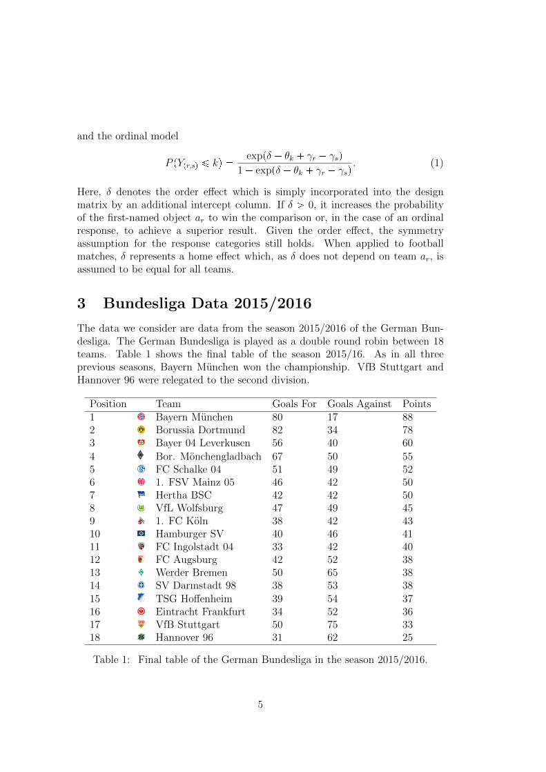
The data we consider are data from the season 2015/2016 of the German Bun-desliga. The German Bundesliga is played as a double round robin between 18teams. Table 1 shows the final table of the season 2015/16. As in all threeprevious seasons, Bayern Munchen won the championship. VfB Stuttgart andHannover 96 were relegated to the second division.

Position Team Goals For Goals Against Points1 Bayern Munchen 80 17 882 Borussia Dortmund 82 34 783 Bayer 04 Leverkusen 56 40 60

4 Bor. Monchengladbach 67 50 555 FC Schalke 04 51 49 526 1. FSV Mainz 05 46 42 507 Hertha BSC 42 42 508 VfL Wolfsburg 47 49 459 1. FC Koln 38 42 4310 Hamburger SV 40 46 4111 FC Ingolstadt 04 33 42 4012 FC Augsburg 42 52 3813 Werder Bremen 50 65 3814 SV Darmstadt 98 38 53 38

15 TSG Hoffenheim 39 54 3716 Eintracht Frankfurt 34 52 3617 VfB Stuttgart 50 75 3318 Hannover 96 31 62 25

Table 1: Final table of the German Bundesliga in the season 2015/2016.

5

All 306 matches played on the 34 match-days of this season will be consideredas the observations in the data set. We will treat a match as a paired comparisonof both teams with respect to their playing abilities. The response variables Yipr,sqrepresent the outcome of a match between team ar (as the home team) and teamas on matchday i. We use a 5-point scale defined by

Yipr,sq �

$''''''&''''''%

1 if team ar wins by at least 2 goals difference,

2 if team ar wins by 1 goal difference,

3 if the match ends with a draw,

4 if team as wins by 1 goal difference,

5 if team as wins by at least 2 goals difference.

Model (1) is able to handle such ordinal response categories. Fitted to theBundesliga data of the season 2015/16, the model yields ability estimates aspresented in Table 2. Additionally, estimates of the threshold parameters θ1 ��θ4 � �1.591 and θ2 � �θ3 � �0.576 and the home effect δ � 0.265 wereobtained.

Position Team γr Rank1 BAY Bayern Munchen 1.899 12 DOR Borussia Dortmund 1.598 23 LEV Bayer 04 Leverkusen 0.433 4

4 MGB Bor. Monchengladbach 0.475 35 S04 FC Schalke 04 0.133 56 MAI 1. FSV Mainz 05 0.088 67 BER Hertha BSC -0.001 78 WOB VfL Wolfsburg -0.142 99 KOE 1. FC Koln -0.045 8

10 HSV Hamburger SV -0.183 1011 ING FC Ingolstadt 04 -0.228 1112 AUG FC Augsburg -0.363 1313 BRE Werder Bremen -0.361 1214 DAR SV Darmstadt 98 -0.467 15

15 HOF TSG Hoffenheim -0.448 1416 FRA Eintracht Frankfurt -0.623 1617 STU VfB Stuttgart -0.699 1718 HAN Hannover 96 -1.068 18

Table 2: Ability estimates for single teams considering model (1)

The ranking of the estimated abilities more or less coincides with the rankingsof the final table. After all, there are a few interesting differences. For example,Borussia Monchengladbach is assessed to be on rank 3 according to the estimated

6

ability 0.475. However, the team finished the season on position 4 and, in contrastto the third-placed Bayer 04 Leverkusen, has to play qualification matches forthe participation in the UEFA Champions League.

Nowadays, in professional football matches a huge amount of variables is col-lected. For example, for every team it is known what distance the team ranin a certain match or its number of shots on goal. The main goal of this workis to determine the influence of these match-specific variables. In the GermanBundesliga, the data supplier opta (http://www.optasports.com/) provides in-teresting data collections. The data we use are freely available from the website ofthe German football magazine kicker (http://www.kicker.de/), Table 3 showsa short excerpt of the data including the first three matches of the season.

Match Goals Home Team Distance Shots on Goal . . .

1 5 yes Bayern Munchen 109 23 . . .1 0 no Hamburger SV 111 5 . . .

2 2 yes Bayer 04 Leverkusen 116 25 . . .

2 1 no TSG Hoffenheim 116 6 . . .

3 0 yes FC Augsburg 106 20 . . .3 1 no Hertha BSC 04 111 11 . . .

......

......

......

. . .

Table 3: Exemplary extract of the Bundesliga data basis from http://www.

kicker.de/

From these (original) data, the ordinal responses for the paired comparisons(as described above) were derived. In detail, the following variables are available(per team and per match):

Home Dummy variable for home team

Distance Total amount of km run

BallPossession Percentage of ball possession

TacklingRate Rate of won tacklings

ShotsonGoal Total number of shots on goal

Passes Total number of passes

Misplaced Total number of misplaced passes (not reaching teammates)

CompletionRate Percentage of passes reaching teammates

7

Hom

e

Dis

tan

ce

BallP

oss

essi

on

Tack

lin

gR

ate

Sh

ots

on

Goal

Com

ple

tion

Rate

Fou

lsS

uff

ered

Off

sid

e

Home 1.000Distance 0.035 1.000

BallPossession 0.102 -0.113 1.000TacklingRate 0.102 -0.082 0.186 1.000ShotsonGoal 0.230 0.042 0.519 0.261 1.000

CompletionRate 0.068 0.103 0.717 0.118 0.422 1.000FoulsSuffered 0.067 -0.200 0.089 0.236 0.035 -0.160 1.000

Offside 0.038 -0.037 0.091 0.088 0.055 0.042 -0.011 1.000

Table 4: Correlation matrix for all used variables and home effect

Fouls Number of fouls or hands

FoulsSuffered Number of fouls suffered

Offside Number of offsides (in attack)

Obviously, some of these variables are correlated or even simple transforma-tions of each other and, therefore, not all of the variables should be included intoa regression analysis. As the variable Fouls is equal to the variable FoulsSuf-fered of the respective opponent (except for hands), only FoulsSuffered will beused. CompletionRate can be calculated as the ratio Passes�Misplaced

Passesand seems

to be a sensible and very informative variable for the passing behavior of a team.Also, Passes is highly correlated with BallPossession with an overall correlationof 0.88 and team-specific correlations up to 0.92 for Hertha BSC Berlin. There-fore, Passes and Misplaced were excluded from the analysis. Table 4 containsthe correlation matrix for all remaining variables from the data set. Note thatTable 4 was generated by considering the overall pairwise correlations of the vari-ables, over all the 34 matches and the 18 teams. It can be seen that, due to thehigh correlation between Passes and BallPossession also CompletionRate andBallPossession are correlated, but not too strongly.

4 A Paired Comparison Model Including Match-

specific Covariates

In general, in paired comparison data one has to distinguish between objects andsubjects. The objects in paired comparisons are the entities that are comparedwith respect to a certain underlying latent (or non-observable) trait. In footballmatches, the objects are the teams that are compared with respect to their playingabilities. The subjects are the entities that perform the respective comparison.For example, in marketing studies one often tries to determine the attractiveness

8

of several products by presenting pairs of the products to participants. Then,the participant (who is the subject of the paired comparison) has to decide whichproduct is more attractive to him. In football matches, a single match itself or amatch-day, respectively, can be seen as the subject that performs the comparison.The distinction between objects and subjects is particularly important when itcomes to the inclusion of covariates. Covariates in paired comparisons can vary

• only over the subjects (subject-specific)

• only over the objects (object-specific)

• both over the subjects and the objects (subject-object-specific).

For each type of covariates, different modeling strategies are necessary. Thevariables that will be considered in the following (and are introduced in Section 3)vary both over the teams and the matchdays and, therefore, can be regarded assubject-object-specific covariates.

4.1 Model Specification

In the following, a model is proposed that is able to include match-specific covari-ates. The starting point is the basic model (1), which is able to handle orderedresponse values (including draws) together with a global order effect. In the con-text of football matches the order effect is considered as the home effect, i.e. the(possible) advantage a team has over its opponent if playing at the home ground.The order effect δ in model (1) is a global order effect which does not vary acrossobjects. In our extended model, δ is replaced by δr so that home effects areteam-specific instead of being global effects equal for all teams.

Another and more important extension is the inclusion of match-specific, or,more technical, subject-object-specific covariates zir. The covariates are incorpo-rated into the model with object-specific parameters αr. As the covariates varyover the subjects (matches) i, also the playing abilities γir and the response Yiprsqnow have to depend on the specific match. For that purpose, we propose to usethe general model for ordinal response data Yipr,sq P t1, . . . , Ku

P pYipr,sq ¤ kq �exppδr � θk � γir � γisq

1 � exppδr � θk � γir � γisq

�exppδr � θk � βr0 � βs0 � z

Tirαr � z

Tisαsq

1 � exppδr � θk � βr0 � βs0 � zTirαr � z

Tisαsq

, (2)

assuming that the abilities in match i are given by γir � βr0�zTirαr. Altogether,

the linear predictor of the model contains the following terms:

δr team-specific home effects of team ar

9

θk category-specific threshold parameters

βr0 team-specific intercepts

zir p-dimensional covariate vector that varies over teams and matches

αr p-dimensional parameter vector that varies over teams.

In contrast to the playing abilities γr from model (1) the playing abilities are nowextended by covariate effects.

4.2 Estimation and Penalization

The team-specific home effects and the inclusion of team-match-specific covariatesleads to a huge increase of the model complexity. Therefore, it is reasonable toinclude penalty terms into the estimation procedures. The goal is to end up witha model with a moderate complexity only using the parameters that are reallyneeded. In general, a penalized version lpp�q � lp�q � λJp�q of the likelihood lp�qwill be maximized considering a general penalty term Jp�q controlled by a tuningparameter λ. In particular, L1-type penalties on differences of coefficients will beused.

Both the home effect and the covariate effects could also be included as globalparameters instead of team-specific parameters. To decide, whether the home ef-fect or single covariate effects should be considered with team-specific or globalparameters, penalty terms with respect to all pairwise differences of the respec-tive parameters will be used. Such a penalty is able to set differences betweenparameters to exactly zero and, therefore, to find clusters of teams with equaleffects. Furthermore, it is also possible that single covariates have no effect at alland are excluded from the model completely.

First, the penalty term for the home effects is considered. Penalizing allpairwise absolute differences leads to the penalty term

Pδpδ1, . . . , δmq �¸r s

|δr � δs|. (3)

As stated before, the penalty can lead to differences of exactly zero so that δr � δsfor r, s P t1, . . . ,mu. If several differences are set zero, one gets clusters of teamswith equal home effects. In the most extreme case (λ Ñ 8), all differences areestimated to be zero which leads to a model with a global home effect δ � δ1 �. . . � δm equal across all teams. As there is no doubt about the general presenceof a home effect in national league football, no additional penalty on the absolutevalues of the home effects is applied.

Second, the penalty term for the covariate effects is considered. Here, in addi-tion to all pairwise absolute differences between the parameters that correspond

10

to one covariate, also all absolute values are penalized using the penalty term

Pαpα1, . . . ,αmq �p

j�1

¸r s

|αrj � αsj| �p

j�1

m

r�1

|αrj|. (4)

In contrast to the home effect, for the other covariates it is not known in advanceif a certain covariate is influential at all. Therefore, an additional penalty onthe absolute values is introduced. Now, in the most extreme case (λ Ñ 8) allcovariates are excluded completely from the model. With a decreasing tuningparameter λ, single covariates enter the model, either with equal effects for allteams or with different clusters of teams.

Both penalties are combined resulting in a joint penalty term Jp�q � Pδp�q �Pαp�q. In general, the tuning parameter λ bridges between two extreme models,namely model (1) and model (2). While model (1) contains a global home effectand no covariate effects at all, model (2) contains (different) team-specific homeand covariate effects. Starting from model (1), the team-specific playing abilitiesγr coincide with the team-specific intercepts βr0 from model (2). With decreasingtuning parameter λ, additional covariate effects enter the model. In general, itcan be assumed that there is a strong correlation between some covariates andthe team-specific intercepts. For example, stronger teams certainly have (onaverage) higher values for the shots on goal than weaker teams. As, in contrastto the covariate effects, the intercepts are not penalized, in such a case the effectof the shots on goal is already covered by the regular team-specific intercepts.Therefore, the covariate effects can be seen as extensions of the playing abilities,containing additional effects that are not yet covered by those. In that sense, thecovariate effects can help to explain (unexpected) match results which can notfully be explained solely by the team-specific intercepts. As the (unpenalized)team-specific intercepts can be expected to cover most of the abilities of theteams, the covariates only become relevant if teams over- (or under-)perform incertain matches. In order to investigate how the team abilities depend on thesingle covariates, in Section 5 a second model without team-specific intercepts isapplied to the data.

In order to achieve comparable effects of the different penalty terms on theparameters of the different covariates, the covariates have to be transformed intoa common scale. For that purpose, all values corresponding to the home effectand the covariates (across all matches and all teams) are scaled to a variance ofone. Consequently, due to the scaling the magnitude of parameter estimates iscomparable between different covariates.

In general, for regularization techniques a crucial point is the determinationof the optimal tuning parameter. Mostly, two different strategies can be applied,namely model selection criteria (e.g. AIC or BIC) or cross-validation. WhileAIC or BIC use the models complexity in terms of the degrees of freedom ofthe models, cross-validation is solely based on out-of-sample prediction. While

11

the determination of the degrees of freedom is lively discussed for different mod-els (and regularization techniques), cross-validation is applicable in almost allcircumstances. Therefore, in this work the optimal tuning parameter λ is deter-mined by 10-fold cross-validation with respect to the so-called ranked probabilityscore (RPS). The RPS for ordinal response y P t1, . . . , Ku (Gneiting and Raftery,2007) can be denoted by

RPSpy, πpkqq �K

k�1

pπpkq � 1py ¤ kqq2,

where πpkq represents the cumulative probability πpkq � P py ¤ kq. In contrastto other possible error measures (e.g. the deviance), it takes the ordinal structureof the response into account.

4.3 Results

For easier interpretation of the intercepts, the covariates were centered (per teamaround the team-specific means). Centering the covariates only changes the paths(and interpretation) of the team-specific intercepts. Now, a team-specific inter-cept represents the ability of a team if all covariates are assumed to be equal tothe team-specific means. The paths and the interpretation of the covariate effectsremain unchanged, representing the effect of a covariate for the team ability whenthe respective covariate changes.

Figure 1 shows the coefficient paths for all parameter estimates (except thethreshold parameters θk) along (a transformation of) the tuning parameter λ. Allpaths corresponding to one covariate are collected in a separate plot. For a largetuning parameter λ, the home effects start with one joint cluster of all teams and(with decreasing λ) end up with separate home effects for all teams. Similarly, allcovariate effects start with an effect of zero and end up with separate effects for allteams. As the intercept parameters are not penalized, they only vary due to thechanges of the covariate effects. Consequently, for large λ model (1) and for λ � 0the unpenalized model (2) is obtained, respectively. In general, the clusteringeffect of the penalty becomes obvious. For example, for the covariate Distancea joint cluster of all teams is formed with decreasing tuning parameters. Incontrast, for CompletionRate only single teams like Bayern Munchen and BorussiaDortmund form clusters of their own. The dashed vertical lines represent theoptimal model according to the 10-fold cross-validation. Compared to the mostcomplex model possible, the complexity of the final model found by the cross-validation is clearly reduced. Figure 2 shows the results of the cross-validationalong the tuning parameter λ.

Table 5 shows all final parameter estimates (for the model chosen by cross-validation) separately per team and per covariate. Distance has the largest effectsamong all covariates, it takes the value 1.01 for all teams. Therefore, in general

12

2.0 1.5 1.0 0.5 0.0

0.0

0.5

1.0

1.5

2.0

Home

log(λ + 1)

HOF

HSVBRELEVMAIKOES04

HANFRAAUGBAYDARSTU

BERMGBDOR

INGWOB

2.0 1.5 1.0 0.5 0.0

−4

−2

02

46

Intercept

log(λ + 1)

INGDAR

HAN

STUFRABREAUG

HSVLEVBERHOFKOE

MAI

WOBS04MGB

DOR

BAY

2.0 1.5 1.0 0.5 0.0

0.0

0.5

1.0

1.5

2.0

2.5

Distance

log(λ + 1)

BAY

HOFBERS04

STUWOB

BREAUGHANLEVKOE

MGBDORFRAHSVINGDARMAI

2.0 1.5 1.0 0.5 0.0

−4

−3

−2

−1

0

BallPossession

log(λ + 1)

DARHSV

STU

BAY

DORFRA

BRES04MAIHOFLEVAUG

KOEBERINGWOBMGBHAN

2.0 1.5 1.0 0.5 0.0

−0.

50.

00.

51.

01.

5

TacklingRate

log(λ + 1)

DAR

BAY

STU

BERS04DORFRALEVHSVMAIBREINGHANAUGKOEHOFWOB

MGB

2.0 1.5 1.0 0.5 0.0

−1.

0−

0.5

0.0

0.5

1.0

ShotsonGoal

log(λ + 1)

KOE

HOF

WOBINGLEVMGBHAN

BAYDARDORFRAS04HSV

STUAUG

BERBREMAI

2.0 1.5 1.0 0.5 0.0

02

46

CompletionRate

log(λ + 1)

HAN

AUG

INGMAIKOEDAR

BERS04HSVHOFBREFRA

WOBLEVSTUMGB

DOR

BAY

2.0 1.5 1.0 0.5 0.0

−0.

50.

00.

51.

0

FoulsSuffered

log(λ + 1)

BAYBERBRE

AUGHOFMGB

HAN

DORSTUDARHSV

WOB

FRALEVMAI

KOEING

S04

2.0 1.5 1.0 0.5 0.0

−1.

0−

0.5

0.0

0.5

Offside

log(λ + 1)

INGBER

HOF

BAYBREDARWOBKOESTUFRA

HSV

HANAUGDORS04

LEVMAIMGB

Figure 1: Coefficient paths (along sequence of λ) for model (2) separately forall covariate effects. Dashed vertical lines represent optimal model according to10-fold cross-validation.

a better (worse) running performance of a team clearly improves (diminishes)the chances of the team for a good result. The second largest effect corresponds

13

2.0 1.5 1.0 0.5 0.0

180

200

220

240

260

280

log(λ + 1)

RP

S

Figure 2: Cross-validation error along tuning parameter λ for model (2). Dashedvertical line represents optimal model according to 10-fold cross-validation.

to the covariate BallPossession. Interestingly, it has a negative effect for allteams. However, one has to keep in mind that there are correlations betweensome covariates. In particular, the variables BallPossession and CompletionRateare fairly correlated. For Borussia Dortmund and, especially for Bayern Munchen,the team-specific effects of the CompletionRate are positive and, therefore, actcontrarily to the negative effect of BallPossession. Furthermore, a positive homeeffect and a positive effect for the TacklingRate are estimated for all teams. Thecovariates ShotsonGoal, FoulsSuffered and Offside are excluded completely fromthe final model. While this result might have been expected for the latter twovariables, it may seem somewhat surprising for ShotsonGoal. However, one hasto keep in mind that all covariate effects are additional effects to the generalabilities represented by the (unpenalized) team-specific intercepts.

In order to illustrate the overall importance of the single covariate effects,Figure 3 displays the paths of the L2-norms

||pαλ1j, . . . , αλ18jq||

of the single covariates j along the tuning parameter λ. In contrast to Figure 1,in Figure 3 it is easier to compare the magnitude of the different covariate effects.Distance is by far the most influential variable followed by BallPossession.

The covariate effects of model (2) have a very specific interpretation. Everyteam has an (unpenalized) intercept that reflects the average ability of the teamover the season. Therefore, the intercepts already cover the mean covariate ef-fects of all teams. Accordingly, the covariate effects captured in the respectiveparameter vectors αr represent effects where covariates can explain deviationsof the performance of a team from its average performance. This fact has to bekept in mind for the interpretation of the covariate effects from model (2).

14

Hom

e

Inte

rcep

t

Dis

tance

Bal

lPos

sess

ion

Tac

klingR

ate

Shot

sonG

oal

Com

ple

tion

Rat

e

Fou

lsSuff

ered

Off

side

AUG 0.34 -0.71 1.01 -0.75 0.22 0.00 0.00 0.00 0.00BAY 0.34 3.53 1.01 -0.75 0.22 0.00 1.99 0.00 0.00BER 0.34 0.14 1.01 -0.75 0.22 0.00 0.00 0.00 0.00BRE 0.34 -0.81 1.01 -0.75 0.22 0.00 0.00 0.00 0.00DAR 0.34 -2.21 1.01 -0.75 0.22 0.00 0.00 0.00 0.00DOR 0.34 2.15 1.01 -0.75 0.22 0.00 0.27 0.00 0.00FRA 0.34 -1.03 1.01 -0.75 0.22 0.00 0.00 0.00 0.00HAN 0.34 -1.40 1.01 -0.75 0.22 0.00 0.00 0.00 0.00

HOF 0.34 -0.42 1.01 -0.75 0.22 0.00 0.00 0.00 0.00HSV 0.34 -0.27 1.01 -0.75 0.22 0.00 0.00 0.00 0.00ING 0.34 -1.10 1.01 -0.75 0.22 0.00 0.00 0.00 0.00

KOE 0.34 -0.05 1.01 -0.75 0.22 0.00 0.00 0.00 0.00LEV 0.34 0.15 1.01 -0.75 0.22 0.00 0.00 0.00 0.00MAI 0.34 0.28 1.01 -0.75 0.22 0.00 0.00 0.00 0.00

MGB 0.34 1.46 1.01 -0.75 0.22 0.00 0.00 0.00 0.00S04 0.34 0.37 1.01 -0.75 0.22 0.00 0.00 0.00 0.00

STU 0.34 -0.85 1.01 -0.75 0.22 0.00 0.00 0.00 0.00WOB 0.34 0.75 1.01 -0.75 0.22 0.00 0.00 0.00 0.00

Table 5: Parameter estimates of Model (2) at optimal tuning parameter accord-ing to 10-fold cross-validation.

5 Alternative Modeling Approach for Covariate

Effects

If one is interested in the total effect of a covariate on the performance of singleteams, a different parameterization seems appropriate. In an alternative ap-proach, the team-specific intercepts are simply eliminated from the model. Inthis parametrization, the specific ability of team ar on matchday i is specified byγir � zT

irαr instead of γir � βr0 � zTirαr as in model (2). Therefore, with this

alternative parameterization the model can be denoted by

P pYipr,sq ¤ kq �exppδr � θk � γir � γisq

1 � exppδr � θk � γir � γisq

�exppδr � θk � z

Tirαr � z

Tisαsq

1 � exppδr � θk � zTirαr � z

Tisαsq

. (5)

15

2.0 1.5 1.0 0.5 0.0

01

23

45

67

log(λ + 1)

FoulsSuffered

ShotsonGoalOffside

Tackling

CompletionRate

BallPossession

Distance

Figure 3: Variable importance with respect to the L2 norms of the variable-specific parameter vectors for model (2) along tuning parameter λ.

In this alternative approach, the mean abilities of the teams cannot be coveredby the team-specific intercepts and have to be replaced by covariate effects. Thisalso implies that in this alternative model the average values of the covariates foreach team are relevant and, hence, the covariates are not centered per team andcovariate but only per covariate. Although the team-specific intercepts βr0 arenow eliminated, model (5) can still become highly complex if for each team andcovariate separate effects are estimated. Therefore, again the penalty terms (3)and (4) are used for estimation.

Figure 4 shows the coefficient paths of model (5) along the tuning parameter λ,the dashed vertical lines represent the optimal model according to 10-fold cross-validation. Similar to the effects estimated for model (2), positive effects forDistance and (mostly) negative effects for BallPossession are found. Now, forboth covariates we see different clusters of teams with equal effects. For examplefor Distance, Bayern Munchen and Hannover 96 have slightly smaller effects thanall the other teams. For CompletionRate, again Bayern Munchen and BorussiaDortmund stand out. Only FoulsSuffered is eliminated completely from themodel, all other covariates have effects for at least some of the teams.

In contrast to model (2), here the covariates were not centered per team inadvance to the analyses, but only globally per covariate. This is due to the factthat in model (2) team-specific differences would all be captured in the inter-cepts. In model (5), no intercepts exist and differences between the teams withrespect to the absolute levels of the covariates do matter. In Figure 5, the mean

16

2.0 1.5 1.0 0.5 0.0

−1

01

2

Home

log(λ + 1)

HOFHSV

FRABRELEV

DARHANS04MAIDOR

KOEAUGBER

STUBAYINGWOB

MGB

2.0 1.5 1.0 0.5 0.0

0.0

0.5

1.0

1.5

2.0

2.5

3.0

Distance

log(λ + 1)

BAYHAN

S04

WOBHOFAUGMGBKOEBERSTULEVBREMAIHSVFRA

INGDARDOR

2.0 1.5 1.0 0.5 0.0

−4

−3

−2

−1

0

BallPossession

log(λ + 1)

HSVDORSTUMAIFRABAYBREHOFHANS04AUGLEVDARBERKOEINGWOB

MGB

2.0 1.5 1.0 0.5 0.0

−1.

5−

0.5

0.5

1.5

TacklingRate

log(λ + 1)

DAR

BAY

LEV

STUS04FRAHANDORHOFHSVINGBERKOEMAIAUG

BREWOBMGB

2.0 1.5 1.0 0.5 0.0

−2

−1

01

2

ShotsonGoal

log(λ + 1)

KOE

WOBMGBFRAINGSTUDARBERHOFLEVBAYAUGHSVHANBRES04

DORMAI

2.0 1.5 1.0 0.5 0.0

02

46

8

CompletionRate

log(λ + 1)

AUGMAIKOEHSVHANDARHOFLEVBERFRASTUINGBRES04MGBWOB

BAYDOR

2.0 1.5 1.0 0.5 0.0

−0.

50.

00.

51.

0

FoulsSuffered

log(λ + 1)

MGBAUG

BAYSTUWOBBREDARMAIS04HSVHANBERHOF

INGFRA

DORKOE

LEV

2.0 1.5 1.0 0.5 0.0

−1.

00.

01.

02.

0

Offside

log(λ + 1)

BERKOE

INGHOFBREWOBDARAUGFRASTU

S04BAYHSVDORHANLEVMAI

MGB

Figure 4: Coefficient paths (along relevant sequence of λ) for alternative model(5), separately for all covariate effects. Dashed vertical lines represent optimalmodel according to 10-fold cross-validation.

effect of the respective covariates together with the single parameter estimatesis illustrated. In these so-called effect stars (Tutz and Schauberger, 2013) onecan see the average covariate values (per team, per covariate) multiplied by therespective parameter estimates. Therefore, these values represent the averagecontribution of a covariate to the ability of a single team. More precisely, theeffect stars show the exponentials of the product of average covariate values andparameter estimates. Per effect star, a circle with radius expp0q � 1 is drawn rep-resenting the no-effect case. Values within the circle represent negative (average)

17

AUG

BAY

BERBREDAR

DORFRAHAN

HOF

HSV

ING

KOELEV

MAIMGB

S04

STU

WOB

Distance

AUG

BAY

BER

BRE

DAR

DORFRA

HAN

HOF

HSV

ING

KOELEV

MAI MGBS04

STU

WOB

BallPossession

AUG

BAY

BER

BREDAR

DOR

FRA

HAN

HOF

HSV

ING

KOE

LEVMAI MGB

S04

STU

WOB

Tackling

AUG

BAY

BER

BREDARDOR

FRA

HAN

HOF

HSV

ING

KOE

LEVMAI MGB

S04

STU

WOB

Shots

AUG

BAY

BER

BREDARDOR

FRA

HAN

HOF

HSV

ING

KOE

LEVMAI MGB

S04

STU

WOB

FoulsSuffered

AUG

BAY

BER

BREDARDOR

FRA

HAN

HOF

HSV

ING

KOE

LEVMAI MGB

S04

STU

WOB

Offside

Figure 5: Effect stars for (average) covariate effects for model (5)

18

effects for the team ability, values beyond the circle represent positive (average)effects for the team ability. The effect star for completion rate is displayed ona different scale for better visibility. It can be seen that (together with its highmean value of CompletionRate) Bayern Munchen has a huge positive effect ofCompletionRate for the team ability, it is the variable that at most distinguishesBayern Munchen from the rest of the league. Also Borussia Dortmund has a bigeffect of CompletionRate. Compared to these two effects, all other effects seemsnegligible at first sight, but there are some noticeable effects for BallPossessionand especially for Distance.

6 Assessment of Model Performances

Finally, it is desirable to assess the performance of the basic model (1) and thetwo proposed models (2) and (5). Beside comparing the models with each other,it can also be interesting to see if the models can compete with bookmakers’ odds.Bookmakers’ odds are known before the respective matches and aggregate mostof the information that is known in advance of a match (including informationnot available in our data like injuries or presumable team line-ups). The Websitehttp://www.football-data.co.uk provides odds averaged over different bookmak-ers. After eliminating the bookmakers margins, these odds are easily transformedinto probabilities. In contrast to the bookmakers’ odds, models (2) and (5) usecovariate data which are only known after the match. Therefore, the bookmak-ers’ odds can serve as a good benchmark. If the proposed models outperform thebookmakers’ odds, this is a clear hint that the covariate information is used in asensible manner to gain more knowledge. Of course, in practice the models cannot be used for prediction as the respective covariate information is only availableafter a match.

The comparison of the different match predictions is performed in the follow-ing manner. To prevent effects of overfitting, the predictive power of the threemodels is assessed using a leave-one-out strategy. Step by step, the models arefitted (and optimized) on training data consisting of 33 matchdays. One match-day at a time is left out of the training data and the corresponding nine matchesare used for prediction. To make our predictions (5 categories) compatible to thebookmakers’ odds (3 categories for victory home team, draw and victory awayteam), the predictions are reduced to the respective 3 categories merging cate-gories 1 and 2 and categories 4 and 5 of the response variables. In total, oneends up with 3 probabilities for each of the 306 matches of the season, separatelyfor the three models and the bookmakers’ odds. Per match, the probability ofthe true match outcome is stored. Table 6 contains the mean probabilities for acorrect (out-of-sample) prediction for the three approaches and the bookmakers’odds:

Moreover, Figure 6 illustrates boxplots of the differences of the single pre-

19

Model (1) Model (2) Model (5) Bookmakers42.0% 49.8% 43.3% 41.9%

Table 6: Average (out-of-sample) probabilities for a correct match prediction

dictions of the three models compared to the bookmakers odds. Here, positivevalues represent matches with a better prediction compared to the bookmakers’odds.

●●●●

●

●

●

●

●

●

●

●

●

●

●

●

●

●●

●●●

●

●

●

●●●

●

●

●

●●

●

●●●

●

●

●

●

●

●

●

●●

Model (1) Model (2) Model (5)

−0.

4−

0.2

0.0

0.2

0.4

0.6

Figure 6: Boxplots of differences comparing out-of-sample predictions for realizedmatch results with betting odds

As pointed out before, the bookmakers odds and the models use differentinformation. After all, it can be seen that the predictive performance of model (2)outperforms all other approaches. Also models (1) and (5) can compete with thebookmakers’ odds. This is surprising, as model (1) only uses mean abilities overthe whole season (except for the predicted matchday) and, therefore, does notcontain any match-specific information, in contrast to the bookmakers. On theother hand, the ability estimates of model (5) are solely based on match-specificcovariate information without any component regarding the overall strength of ateam. Also this model competes well with the bookmakers odds.

20

7 Concluding Remarks

This work deals with data from the German Bundesliga from the season 2015/16and considers several match-specific variables in a paired comparison model. Theproposed model is an attempt to make use of the big amount of data that iscollected in modern football and to simultaneously connect the correspondingvariables to the outcome of the matches. Due to the fact that the used covariatesare correlated, a simultaneous modeling approach seems sensible. After all, com-plex modeling approaches are rather scarce in this area. The model treats thematches of the respective season of the German Bundesliga as paired compar-isons between the competing teams, comparing the playing abilities of the teamsusing ordinal responses. The variables are, in a linear way, incorporated into theplaying abilities of the teams in specific matches. In future work also non-lineareffects might be worth considering. The model can easily be applied to data fromother leagues or other types of sport.

Overall, the variable Distance turned out to be the most important variableamong all considered variables. This finding endorses the widely spread beliefthat a good running performance of a team is the most important premise fora successful match. The variable TacklingRate also turned out to have the ex-pected positive effect, although it is much smaller than the effect of Distance. Incontrast, the finding of a negative effect of BallPossession seems to be rathercounter-intuitive. Maybe, this finding reflects a new trend in the German Bun-desliga (started by Borussia Dortmund and Jurgen Klopp) to focus on fast counterattacks rather than on long (and rather slow) periods of permanent ball posses-sion. After all, for Bayern Munchen one might also argue that they have a strongpositive effect of CompletionRate which is quite strongly (positively) correlatedto BallPossession. Therefore, this finding might in fact also represent a positiveeffect of BallPossession for Bayern Munchen.

The comparison of the model performance to bookmakers’ odds shows that thevariables actually carry information and clearly improve the model in contrastto a model without covariate effects and that the model also outperforms thebookmakers odds. Therefore, the model seems to be a promising approach tomake use of the big amount of data available in football and to better understandthe effect of the single covariates for the success of teams.

References

Agresti, A. (1992). Analysis of ordinal paired comparison data. Applied Statis-tics 41 (2), 287–297.

Agresti, A. (2002). Categorical Data Analysis. New York: Wiley.

21

Bradley, R. A. and M. E. Terry (1952). Rank analysis of incomplete block designs,I: The method of pair comparisons. Biometrika 39, 324–345.

Carmichael, F., D. Thomas, and R. Ward (2000). Team performance: the caseof English Premiership football. Managerial and Decision Economics 21 (1),31–45.

Casalicchio, G., G. Tutz, and G. Schauberger (2015). Subject-specific Bradley-Terry-Luce models with implicit variable selection. Statistical Modelling 15 (6),526–547.

Castellano, J., D. Casamichana, and C. Lago (2012). The use of match statisticsthat discriminate between successful and unsuccessful soccer teams. Journalof human kinetics 31, 137–147.

Cattelan, M. (2012). Models for paired comparison data: A review with emphasison dependent data. Statistical Science 27 (3), 412–433.

Collet, C. (2013). The possession game? A comparative analysis of ball retentionand team success in European and international football, 2007-2010. Journalof Sports Sciences 31 (2), 123–136.

Davidson, R. (1970). On extending the Bradley-Terry model to accommodateties in paired comparison experiments. Journal of the American StatisticalAssociation 65, 317–328.

Dixon, M. J. and S. G. Coles (1997). Modelling association football scores andinefficiencies in the football betting market. Journal of the Royal StatisticalSociety: Series C (Applied Statistics) 46 (2), 265–280.

Dyte, D. and S. R. Clarke (2000). A ratings based Poisson model for WorldCup soccer simulation. Journal of the Operational Research Society 51 (8),993–998.

Francis, B., R. Dittrich, and R. Hatzinger (2010). Modeling heterogeneity inranked responses by nonparametric maximum likelihood: How do europeansget their scientific knowledge? The Annals of Applied Statistics 4 (4), 2181–2202.

Glenn, W. and H. David (1960). Ties in paired-comparison experiments using amodified Thurstone-Mosteller model. Biometrics 16 (1), 86–109.

Gneiting, T. and A. Raftery (2007). Strictly proper scoring rules, prediction, andestimation. Journal of the American Statistical Association 102 (477), 359–376.

22

Groll, A., G. Schauberger, and G. Tutz (2015). Prediction of major internationalsoccer tournaments based on team-specific regularized Poisson regression: Anapplication to the FIFA World Cup 2014. Journal of Quantitative Analysis inSports 11 (2), 97–115.

Hughes, M. and I. Franks (2005). Analysis of passing sequences, shots and goalsin soccer. Journal of Sports Sciences 23 (5), 509–514.

Karlis, D. and I. Ntzoufras (2003). Analysis of sports data by using bivariatePoisson models. The Statistician 52, 381–393.

R Core Team (2015). R: A Language and Environment for Statistical Computing.Vienna, Austria: R Foundation for Statistical Computing.

Rao, P. and L. Kupper (1967). Ties in paired-comparison experiments: A gen-eralization of the Bradley-Terry model. Journal of the American StatisticalAssociation 62, 194–204.

Schauberger, G. (2015). BTLLasso: Modelling Heterogeneity in Paired Compar-ison Data. R package version 0.1-2.

Schauberger, G. and G. Tutz (2015). Modelling heterogeneity in paired compar-ison data - an L1 penalty approach with an application to party preferencedata. Technical Report 183, Department of Statistics, Ludwig-Maximilians-Universitat Munchen, Germany.

Turner, H. and D. Firth (2012). Bradley-Terry models in R: The BradleyTerry2package. Journal of Statistical Software 48 (9), 1–21.

Tutz, G. (1986). Bradley-Terry-Luce models with an ordered response. Journalof Mathematical Psychology 30, 306–316.

Tutz, G. and G. Schauberger (2013). Visualization of categorical response mod-els: From data glyphs to parameter glyphs. Journal of Computational andGraphical Statistics 22 (1), 156–177.

Tutz, G. and G. Schauberger (2015). Extended ordered paired comparison modelswith application to football data from German Bundesliga. AStA Advances inStatistical Analysis 99 (2), 209–227.

Vogelbein, M., S. Nopp, and A. Hokelmann (2014). Defensive transition in soccer- are prompt possession regains a measure of success? A quantitative analysisof German Fußball-Bundesliga 2010/2011. Journal of Sports Sciences 32 (11),1076–1083. PMID: 24506111.

23